Abstract

We consider the possibility that photons of noncommutative QED can make bound states. Using the potential model, developed based on the constituent gluon picture of QCD glue-balls, arguments are presented in favor of existence of these bound states. The basic ingredient of potential model is that the self-interacting massless gauge particles may get mass by inclusion non-perturbative effects.

Keywords: Noncommutative Geometry, Noncommutative Field Theory, Quantum Electrodynamics
PACS No.: 02.40.Gh, 11.10.Nx, 12.20.-m

1 Introduction

In Abelian gauge theories on ordinary space-time, there is no self-coupling between the gauge fields. The best known example is the quantum theory of interaction between electric charges and photons, the so-called QED. The situation is different in non-Abelian theories, and due to the commutator term in the field strength, these theories are involved by direct interaction between the quanta of gauge fields. It is now widely believed that the strong interaction is described by a non-Abelian gauge theory accompanied with proper matter fields as quarks, the so-called QCD. As gluons are the quanta of QCD gauge field, from the very beginning this possibility was considered that if gluons can make bound states free from valance quarks, the so-called glue-balls. Although the properties of glue-balls have been studied for a long time, their existence have not still been approved experimentally.

Recently a great interest has been appeared to study field theories on spaces whose coordinates do not commute. These spaces, as well as the field theories defined on them, are known under the names of noncommutative spaces and theories. In contrast to QED on ordinary space-time, as we briefly review in next section, noncommutative QED is involved by direct interactions between photons. Interestingly one finds the situation very reminiscent to that of non-Abelian gauge theories, and then the question is whether there are some kinds of bound states in analogy with glue-balls of QCD, here might be called “photo-ball”s. It is this question that we consider in this work. Our approach to study photo-balls is based on one of methods that has been developed for glue-balls. As glue-balls are non-perturbative in nature, there is still no systematic way for calculation of their properties from the first principles of QCD. Instead, among the years many approaches are developed for extracting glue-ball’s properties, though each approach is based on expectations or estimate calculations.

Among many others, one approach for studying properties of glue-balls has been the so-called constituent gluon model. In any study of bound state of gluons, one is encountered with a situation in which gluons, though at first were introduced massless to the Lagrangian, are bound and do not disjoint to propagate to infinity. Correspondingly, it is argued that quantum fluctuations around a charged particle, that should be treated non-perturbatively in QCD, can make an accompanied cloud for it, causing a dynamically generated mass [1, 2]. Accordingly, it appears very useful to define constituent quarks and gluons, for which we assume a mass of order of bound states of the theory, while their Lagrangian counterparts may be massless or almost massless. As extracting the masses of constituent particles from first principles is not yet done in a satisfactory way, the best evaluations come from estimations based on general considerations, phenomenology or lattice calculations.

Once one accepts that a glue-ball is a bound state of constituent gluons, the question is about the effective theory that captures the interaction between them. One approach is to consider constituent gluons as massive quanta of an effective gauge theory. It needs some kinds of proof, but hopefully this effective gauge theory has the same qualitative features of the true (massless) theory, but in non-perturbative regime [1, 2]. Since it is believed that the main contribution to the mass of a glue-ball is coming from the constituent masses of gluons, it is expected that constituent gluons move non-relativistically inside the glue-ball, and so perturbative calculations for finding the effective potential should be done in non-relativistic regime. Having the effective potential at hand, by studying the Schrodinger-type equations, one can have estimations about mass or size of glue-balls. It is the heart of the potential model approach for studying the properties of the glue-balls [3, 4, 5].

There are two related issues when we are considering the effective gauge theory of constituent gluons as massive vector particles. First, it is known that the gauge symmetry is lost via the mass term, and the second, massive gauge theories are known to be perturbatively non-renormalizable. Here we give comments on these issues [1, 2]. The non-renormalizability of massive gauge theories is under this assumption that the mass in the theory appears as a fixed parameter, surviving at large momentum. In fact the insufficient decrease of propagator of a massive vector particle at large momentum, due to simple power counting, suggests that the theory can not be renormalizable. But the situation might be different in a theory with constituent mass. At very large momentum, where coupling constant is small due to asymptotic freedom, the perturbation is valid and gluons appear as massless particles. So the mass of constituent gluon, which is generated dynamically, depends on momentum and vanishes at large momentum. In a theory for gluons, it is argued that if one can keep the dependence of constituent mass on momentum, which of course is possible only by including the non-perturbative effects, the theory may appear to be non-perturbatively renormalizable.

Although the argument above is for a model involved by dynamically generated mass, due to lack of a systematic treatment of non-perturbative effects, much can be learned via a kinematical description of gluon mass [2]; it is to assume mass as a fix parameter, though the problem still remains with local gauge symmetry. To overcome this problem, there is a prescription that we review briefly in below. Let us consider firstly the case with Abelian symmetry, and QCD case appears just as a generalization [1, 2]. The starting point is the theory given by Lagrangian density:

$$L=-\frac{1}{4}F_{\mu\nu}F^{\mu\nu}+\frac{1}{2}m^{2}\Big{(}A_{\mu}-\frac{1}{g}\partial_{\mu}\varphi\Big{)}^{2}$$ (1)

in which $g$ is the coupling constant, and $\varphi$ is a scalar field. The Lagrangian is invariant under local symmetry

$$A^{\prime}_{\mu}=A_{\mu}-\frac{1}{g}\partial_{\mu}\Lambda,\;\;\;\varphi^{\prime}=\varphi-\Lambda,$$ (2)

with $\Lambda$ as symmetry transformation parameter. Now we see although the gauge field has got mass, the local symmetry is kept. Of course we mention that giving mass is done with the price of introducing an extra scalar field. We have another example of this observation in spontaneous symmetry breaking mechanism, in which we are left with Goldstone bosons. In fact, this extra scalar field, just like their Goldstone boson counterparts, does not appear in the $S$-matrix, i.e. as external legs of diagrams. One may insert the scalar field into the Lagrangian via the obvious solution:

$$\varphi=g\frac{1}{\Box}\partial\cdot A,$$ (3)

getting a non-local but still gauge invariant theory involving only $A_{\mu}$. It is the generalization of this mechanism that has been used for the case of constituent gluon description of QCD glue-balls [3, 4, 5], and here we use for photo-balls of noncommutative QED. The starting point for the QCD case is the Lagrangian density [1, 2]:

$$L=-\frac{1}{4}{\rm Tr}\big{(}F^{\mu\nu}F_{\mu\nu}\big{)}+\frac{1}{2}m^{2}{\rm Tr}\Big{(}A_{\mu}-\frac{1}{g}V(\varphi)\partial_{\mu}V^{\dagger}(\varphi)\Big{)}^{2}$$ (4)

in which

$$V(\varphi)=\exp\Big{[}\frac{i}{2}\sum_{a}T^{a}\varphi_{a}\Big{]}$$ (5)

and $F_{\mu\nu}=\partial_{\mu}A_{\nu}-\partial_{\nu}A_{\mu}-ig[A_{\mu},A_{\nu}]$, with $[T^{a},T^{b}]=if^{ab}_{c}T^{c}$. The action is invariant under

$$A^{\prime}_{\mu} = UA_{\mu}U^{-1}+\frac{1}{g}U\partial_{\mu}U^{-1},$$

$$V(\varphi^{\prime}) = UV(\varphi),$$ (6)

in which $U=U(x)$ is unitary matrix defining the transformation. Again one can insert the scalar fields into the Lagrangian via power series solution in $g$ [1, 2]:

$$\varphi_{a}=g\frac{1}{\Box}\partial\cdot A_{a}-g^{2}[\cdots]_{a}.$$ (7)

As mentioned above the extra scalars do not appear as external legs of diagrams, but the situation is even simpler as far as one considers just the tree diagrams, in which one can ignore the scalars. So for tree diagrams, and in proper gauge, the Lagrangian density in use is practically [2, 4, 5]:

$$L=-\frac{1}{4}F^{a\mu\nu}F^{a}_{\mu\nu}+\frac{1}{2}m^{2}A^{a\mu}A^{a}_{\mu},$$ (8)

simply as a gauge theory for massive gluons.

In the non-relativistic limit the potential can be read off from the total invariant amplitude ${\cal M}_{fi}$ via the Fourier transform [3, 4, 5]:

$$V(\mathbf{r})=\int\frac{{\rm d}^{3}q}{8\pi^{3}}\frac{i{\rm e}^{i\mathbf{q}\cdot\mathbf{r}}}{4\sqrt{E_{1}E_{2}E_{3}E_{4}}}\,i{\cal M}_{fi}$$ (9)

in which $\mathbf{q}$ is the momentum transferred between the in-coming particles. The total invariant amplitude gets contribution at tree level from the s-, t-, u- channels, and the so-called seagull (s.g.) diagram, coming from 4-gluon vertex of QCD [3, 4, 5]. In non-relativistic limit it can be shown that the s-channel’s contribution is ignorable, to get the final expression [3, 4, 5]:

$$i{\cal M}_{fi} = \frac{ig^{2}f^{ace}f^{bde}}{\mathbf{q}^{2}+m^{2}}\times\Big{(}4m^{2}+3\mathbf{q}^{2}-2\mathbf{S}^{2}\mathbf{q}^{2}+2(\mathbf{S\cdot q})^{2}+6i\mathbf{S}\cdot(\mathbf{q}\times\mathbf{p}_{i})\Big{)}$$ (10)

$$-ig^{2}\Big{(}f^{abe}f^{cde}-f^{ace}f^{bde}\big{(}\frac{1}{2}\mathbf{S}^{2}-2\big{)}\Big{)}.$$

By above the gluon-gluon potential in one-gluon-exchange (oge) approximation appears in the form [3, 4, 5]:

$$V_{\rm oge}(\mathbf{r})\!\!\!\! = \!\!\!\!\frac{-g^{2}f^{ace}f^{bde}}{4\pi}\bigg{\{}\Big{[}\frac{1}{4}+\frac{1}{3}\mathbf{S}^{2}-\frac{3}{2m^{2}}(\mathbf{L}\cdot\mathbf{S})\nabla_{r}\bigg{.}-\frac{1}{2}m^{2}\big{(}(\mathbf{S}\cdot\bm{\nabla})^{2}-\frac{1}{3}\mathbf{S}^{2}\nabla^{2}\big{)}\Big{]}\frac{{\rm e}^{-mr}}{r}$$ (11)

$$-\big{(}1-\frac{5}{6}\mathbf{S}^{2}\big{)}\frac{\pi}{m^{2}}\delta^{3}(\mathbf{r})\bigg{\}}+\frac{g^{2}f^{abe}f^{cde}}{4\pi}\frac{\pi}{m^{2}}\delta^{3}(\mathbf{r})$$

in which $\nabla_{r}=r^{-1}\partial_{r}$.

The organization of the rest of this work is as follows. In Sec. 2 we review some basic features of canonical noncommutative spaces, and also the field theories defined on them, specially noncommutative QED. We also remark on some aspects of noncommutative QED that make this theory in some extents similar to QCD. Sec. 3 is devoted to extracting the effective potential between massive photons, by studying the non-relativistic behavior of their scattering. Sec. 4 mainly contains the dynamics of photons under the effective potential obtained in Sec. 3. The existence proof of bound states is also presented in Sec. 4. Sec. 5 is for conclusion and discussions.

2 Noncommutative Space-Time And QED

In last years a great attention is appeared in formulation and studying field theories on noncommutative spaces. One of the original motivations has been to get finite field theories via the intrinsic regularizations which are encoded in some of noncommutative spaces [6]. The other motivation comes back to the natural appearance of noncommutative spaces in some areas of physics, and the recent one in string theory. It has been understood that string theory is involved by some kinds of noncommutativities; two examples are, 1) the coordinates of bound-states of $N$ D-branes are presented by $N\times N$ Hermitian matrices [7], and 2) the longitudinal directions of D-branes in the presence of B-field background appear to be noncommutative, as are seen by the ends of open strings [8, 9, 10]. In the latter case for constant background one simply gets the canonical noncommutative space-time, introduced by commutation relations for coordinates as:

$$[\hat{x}^{\mu},\hat{x}^{\nu}]=i\theta^{\mu\nu}=\frac{i}{\omega^{2}}c^{\mu\nu}$$ (12)

in which the parameter $\omega$ has the dimension of energy, and signifies the scale where noncommutative effects become relevant. The $c^{\mu\nu}$ is a real antisymmetric matrix with elements of order one. Now since the coordinates do not commute, any definition of functions or fields should be performed under a prescription for ordering of coordinates, and one choice can be the symmetric one, the so-called Weyl ordering. To any function $f(x)$ on ordinary space, one can assign an operator $\hat{O}_{f}$ by

$$\hat{O}_{f}\big{(}\hat{x}\big{)}:=\frac{1}{(2\pi)^{n}}\int{\rm d}^{n}k\;\tilde{f}(k)\;{\rm e}^{-ik\cdot\hat{x}}$$ (13)

in which $\tilde{f}(k)$ is the Fourier transform of $f(x)$ defined by

$$\tilde{f}(k)=\int{\rm d}^{n}x\;f(x)\;{\rm e}^{ik\cdot x}.$$ (14)

Due to presence of the phase ${\rm e}^{-ik\cdot\hat{x}}$ in definition of $\hat{O}_{f}$, we recover the Weyl prescription for the coordinates. In a reverse way we also can assign to any symmetrized operator a function or field living on the noncommutative plane. Also, we can assign to product of any two operators $\hat{O}_{f}$ and $\hat{O}_{g}$ another operator as

$$\hat{O}_{f}\cdot\hat{O}_{g}=:\hat{O}_{f\star g}$$ (15)

in which $f$ and $g$ are multiplied under the so-called $\star$-product defined by

$$(f\star g)(x)=\exp\big{(}\frac{i\theta^{\mu\nu}}{2}\partial_{x_{\mu}}\partial_{y_{\nu}}\big{)}f(x)g(y)\mid_{y=x}$$ (16)

By these all one learns how to define physical theories on noncommutative space-time, and eventually it appears that the noncommutative field theories are defined by actions that are essentially the same as in ordinary space-time, with the exception that the products between fields are replaced by $\star$-product; see [11] as review. Though $\star$-product itself is not commutative (i.e., $f\star g\neq g\star f$) the following identities make some of calculations easier:

$$\int f\star g\;{\rm d}^{n}x=\int g\star f\;{\rm d}^{n}x=\int fg\;{\rm d}^{n}x$$

$$\int f\star g\star h\;{\rm d}^{n}x=\int f(g\star h)\;{\rm d}^{n}x=\int(f\star g)h\;{\rm d}^{n}x$$

$$\int f\star g\star h\;{\rm d}^{n}x=\int h\star f\star g\;{\rm d}^{n}x=\int g\star h\star f\;{\rm d}^{n}x$$

By the first two ones we see that, in integrands always one of the stars can be removed. Besides it can be seen that the $\star$-product is associative, i.e., $f\star g\star h=(f\star g)\star h=f\star(g\star h)$, and so it is not important which two ones should be multiplied firstly.

The pure gauge field sector of noncommutative QED is defined by the action

$$S_{\rm gauge-field} = -\frac{1}{4}\int{\rm d}^{4}x\;F_{\mu\nu}\star F^{\mu\nu}$$ (17)

$$= -\frac{1}{4}\int{\rm d}^{4}x\;F_{\mu\nu}F^{\mu\nu}$$

in which the field strength $F_{\mu\nu}$ is

$$F_{\mu\nu}=\partial_{\mu}A_{\nu}(x)-\partial_{\nu}A_{\mu}(x)-ie[A_{\mu}(x),A_{\nu}(x)]_{\star}$$ (18)

by definition $[f,g]_{\star}=f\star g-g\star f$. We mention $[x^{\mu},x^{\nu}]_{\star}=i\theta^{\mu\nu}$. The action above is invariant under local gauge symmetry transformations

$$A^{\prime}_{\mu}(x)\!=\!U\star A_{\mu}(x)\star U^{-1}+\frac{i}{e}U\star\partial_{\mu}U^{-1}$$ (19)

in which $U=U(x)$ is the $\star$-phase, defined by a function $\lambda(x)$ via the $\star$-exponential:

$$U(x)=\exp_{\star}(i\lambda)=1+i\lambda-\frac{1}{2}\lambda\star\lambda+\cdots,$$ (20)

$$U\star U^{-1}=U^{-1}\star U=1$$ (21)

in which $U^{-1}=\exp_{\star}(-i\lambda)$. Under above transformation, the field strength transforms as

$$F_{\mu\nu} \longrightarrow F^{\prime}_{\mu\nu}=U\star F_{\mu\nu}\star U^{-1}$$ (22)

We mention that the transformations of gauge field as well as the field strength look like to those of non-Abelian gauge theories. Besides we see that the action contains terms which are responsible for interaction between the gauge particles, again as the situation we have in non-Abelian gauge theories. We see how the noncommutativity of coordinates induces properties on fields and their transformations, as if they were belong to a non-Abelian theory; the subject that how the characters of coordinates and fields may be related to each other is discussed in [12]. These observations make it reasonable to study whether and how the photons can make bound states in such a theory.

There is another observation that promotes the formal similarities of noncommutative and non-Abelian theories to their behaviors, that is the negative sign of $\beta$-function, which manifests that these theories are asymptotically free [13, 14]. By this it is more reasonable to see if the techniques developed for QCD purposes can also be used for noncommutative QED.

The phenomenological implications of possible noncommutative coordinates have been the subject of a very large number of research publications in last years. Among many others, here we can give just a brief list of works, and specially those concerning the phenomenological implications of noncommutative QED. The effect of noncommutativity of space-time is studied for possible modifications that may appear in high energy scattering amplitudes of particles [15], in energy levels of light atoms [16, 17], and anomalous magnetic moment of electron [18]. The ultra-high energy scattering of massless photons of noncommutative QED is considered in [19] and the tiny change in the total amplitude is obtained as a function of the total energy. Some other interesting features of noncommutative ED and QED are discussed in [20]. The issue of formation of new bound states by space-time noncommutativity has been considered in [21].

3 Massive Noncommutative QED And Effective
Potential Between Photons

3.1 Massive Photon-Photon Scattering Amplitude

Now here, following the procedure developed for QCD case, we give mass to photons of noncommutative QED. As described this is done by introducing an extra scalar field, getting the Lagrangian density:

$$L=L_{\rm gauge-field}+\frac{m^{2}}{2}\Big{(}A_{\mu}+\frac{i}{e}\partial_{\mu}V(\varphi)\star V^{-1}(\varphi)\Big{)}_{\star}^{2}$$ (23)

in which $(\cdots)_{\star}^{2}=(\cdots)\star(\cdots)$, and $V(\varphi)$ is the $\star$-phase defined by the scalar field $\varphi$; see (20). The action defined by above Lagrangian is invariant under transformations

$$A^{\prime}_{\mu}(x)\! = \!U\star A_{\mu}(x)\star U^{-1}+\frac{i}{e}U\star\partial_{\mu}U^{-1}$$

$$V(\varphi^{\prime})\! = \!U\star V(\varphi)$$ (24)

in which $U$ is the same in (19). Now we just list the Feynman rules [2][14, 18]. We choose the gauge in which the propagator takes the form:

$$iD^{\mu\nu}\big{(}p)=\frac{-ig^{\mu\nu}}{p^{2}-m^{2}}+\frac{ip^{\mu}p^{\nu}}{(p^{2}-m^{2})m^{2}}.$$ (25)

In the non-relativistic limit we have for momentum and polarization vectors [4, 5]

$$p^{\mu}=\big{(}m+\frac{\mathbf{p^{2}}}{2m},\mathbf{p}\big{)}$$ (26)

$$\epsilon^{\mu}=\big{(}\frac{\mathbf{p}\cdot\mathbf{e}}{m},\mathbf{e}+\frac{\mathbf{p}\cdot\mathbf{e}}{2m^{2}}\mathbf{p}\big{)}$$ (27)

in which e is a 3-vector satisfying $\mathbf{e}^{*}\cdot\mathbf{e}=1$. From Lorentz condition [3, 4, 5], we have

$$p\cdot\epsilon=p^{\mu}\epsilon_{\mu}=0$$ (28)

In this work we assume for the signature of metric $g_{\mu\nu}=(+1,-1,-1,-1)$.

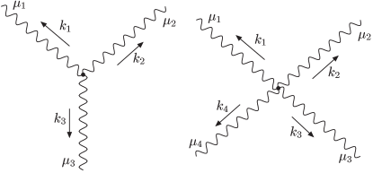
Figure 1: 3- and 4- photon vertices of noncommutative QED.

As in this work we restrict ourselves to tree diagrams, after removing one $\star$, and by Lorentz condition, we practically are using the Lagrangian [2]

$$L=-\frac{1}{4}F^{\mu\nu}F_{\mu\nu}+\frac{1}{2}m^{2}A^{\mu}A_{\mu},$$ (29)

with $F_{\mu\nu}$ defined in (18). There are 3- and 4- photon vertices given in Fig. 1. As in this work we consider noncommutativity just in spatial directions, that is assuming $\theta^{0i}=0$ for $i=1,2,3$, we have for the vertex-functions [14, 18]:

$$\Gamma^{\mu_{1}\mu_{2}\mu_{3}}_{k_{1},k_{2},k_{3}}=-2e\sin\!\big{(}\frac{\mathbf{k}_{1}\ltimes\mathbf{k}_{2}}{2}\big{)}\Big{[}(k_{1}-k_{2})^{\mu_{3}}g^{\mu_{1}\mu_{2}}+(k_{2}-k_{3})^{\mu_{1}}g^{\mu_{2}\mu_{3}}+(k_{3}-k_{1})^{\mu_{2}}g^{\mu_{3}\mu_{1}}\Big{]}$$ (30)

and

$$\Gamma^{\mu_{1}\mu_{2}\mu_{3}\mu_{4}}_{k_{1},k_{2},k_{3},k_{4}}=-4ie^{2}\!\!\!\!\!\!\!\!\! \Big{[}\sin\!\big{(}\frac{\mathbf{k}_{1}\ltimes\mathbf{k}_{2}}{2}\big{)}\sin\!\big{(}\frac{\mathbf{k}_{3}\ltimes\mathbf{k}_{4}}{2}\big{)}\big{(}g^{\mu_{1}\mu_{3}}g^{\mu_{2}\mu_{4}}\!\!-\!g^{\mu_{1}\mu_{4}}g^{\mu_{2}\mu_{3}}\!\big{)}$$ (31)

$$+\sin\!\big{(}\frac{\mathbf{k}_{3}\ltimes\mathbf{k}_{1}}{2}\big{)}\sin\!\big{(}\frac{\mathbf{k}_{2}\ltimes\mathbf{k}_{4}}{2}\big{)}\big{(}g^{\mu_{1}\mu_{4}}g^{\mu_{2}\mu_{3}}\!\!-\!g^{\mu_{1}\mu_{2}}g^{\mu_{3}\mu_{4}}\!\big{)}$$

$$+\sin\!\big{(}\frac{\mathbf{k}_{1}\ltimes\mathbf{k}_{4}}{2}\big{)}\sin\!\big{(}\frac{\mathbf{k}_{2}\ltimes\mathbf{k}_{3}}{2}\big{)}\big{(}g^{\mu_{1}\mu_{2}}g^{\mu_{3}\mu_{4}}\!\!-\!g^{\mu_{1}\mu_{3}}g^{\mu_{2}\mu_{4}}\!\big{)}\Big{]}$$

in which $\mathbf{a}\ltimes\mathbf{b}\equiv\theta^{ij}a_{i}b_{j}$, and the momenta and indices are given in Fig. 1. Also in each vertex energy-momentum conservation should be understood.

Although there are four diagrams at tree level, those coming from s-, t-, u- channels, and seagull diagram (Fig. 2), when extracting the potential, by the properly symmetrized wave function for identical particle systems, the “exchange” or “symmetry” diagrams are automatically taken care of, causing that only one of t- and u- channels’ contributions should be added to others’ contributions [4]. For s-channel we have

$$i{\cal M}^{\rm s}_{fi} = 4e^{2}\sin\!\big{(}\frac{\mathbf{p_{1}}\ltimes\mathbf{k}}{2}\big{)}\sin\!\big{(}\frac{\mathbf{p_{3}}\ltimes\mathbf{k}}{2}\big{)}\epsilon_{1\mu_{1}}\epsilon_{2\mu_{2}}\Gamma^{\mu_{1}\mu_{2}\mu}_{-p_{1},-p_{2},k}$$ (32)

$$\!\Big{(}\frac{-ig_{\mu\nu}}{k^{2}-m^{2}}+\frac{ik_{\mu}k_{\nu}}{(k^{2}-m^{2})m^{2}}\Big{)}\;\Gamma^{\nu\mu_{3}\mu_{4}}_{-k,p_{3},p_{4}}\;\epsilon_{3\mu_{3}}^{*}\epsilon_{4\mu_{4}}^{*}$$

In s-channel we have $k=p_{1}+p_{2}=p_{3}+p_{4}$, and by using it we get

$$i{\cal M}^{\rm s}_{fi} = -4ie^{2}\frac{\sin\!\big{(}\frac{\mathbf{p_{1}}\ltimes\mathbf{k}}{2}\big{)}\sin\!\big{(}\frac{\mathbf{p_{3}}\ltimes\mathbf{k}}{2}\big{)}}{q^{2}-m^{2}}\Big{(}\epsilon_{1}\cdot\epsilon_{2}(p_{1}-p_{2})_{\rho}+2\epsilon_{2\rho}p_{2}\cdot\epsilon_{1}-2\epsilon_{1\rho}p_{1}\cdot\epsilon_{2}\Big{)}$$ (33)

$$\Big{(}\epsilon^{*}_{3}\cdot\epsilon^{*}_{4}(p_{4}-p_{3})^{\rho}-2\epsilon^{*\rho}_{4}p_{4}\cdot\epsilon^{*}_{3}+2\epsilon^{*\rho}_{3}p_{3}\cdot\epsilon^{*}_{4}\Big{)}$$

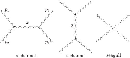
Figure 2: s-channel, t-channel, and seagull diagrams.

From the Lorentz condition the last term in propagator is omitted. By replacing the non-relativistic limit of $\epsilon$’s, we see that, even without considering coefficient involving sin($\cdots$), the leading order contribution of s-channel is order of $|\mathbf{p}|^{2}\ll m^{2}$, that we ignore comparing the zeroth orders. This observation is exactly the same that happens in the QCD case [3, 4, 5].

Now we come to t-channel,

$$i{\cal M}^{\rm t}_{fi}\!=\!\!-4e^{2}\!\sin\!\big{(}\frac{\mathbf{p_{1}}\ltimes\mathbf{q}}{2}\big{)}\!\sin\!\big{(}\frac{\mathbf{p_{2}}\ltimes\mathbf{q}}{2}\big{)}\!\Big{[}g_{\mu\lambda}(p_{1}+p_{3})_{\rho}+g_{\lambda\rho}(p_{1}-2p_{3})_{\mu}+g_{\rho\mu}(p_{3}-2p_{1})_{\lambda}\Big{]}$$

$$\epsilon^{\mu}_{1}\epsilon^{*\lambda}_{3}\frac{-i\big{(}g^{\rho\delta}-\frac{q^{\rho}q^{\delta}}{m^{2}}\big{)}}{q^{2}-m^{2}}\epsilon^{\nu}_{2}\epsilon^{*\sigma}_{4}\Big{[}g_{\nu\sigma}(p_{2}+p_{4})_{\delta}+g_{\sigma\delta}(p_{2}-2p_{4})_{\nu}+g_{\delta\nu}(p_{4}-2p_{2})_{\sigma}\Big{]}$$ (34)

in which $q=p_{3}-p_{1}=p_{2}-p_{4}$. It appears to be useful if we define [4, 5]

$$\langle 3|J_{\rho}|1\rangle=\epsilon^{*}_{3}\cdot\epsilon_{1}(p_{1}+p_{3})_{\rho}-2\epsilon^{*}_{3\rho}p_{3}\cdot\epsilon_{1}-2\epsilon_{1\rho}p_{1}\cdot\epsilon^{*}_{3}$$ (35)

and a similar one for $\langle 4|J^{\delta}|2\rangle$, and since $\langle 3|J_{\rho}|1\rangle q^{\rho}=\langle 4|J_{\delta}|2\rangle q^{\delta}=0$, thus,

$$i{\cal M}^{\rm t}_{fi}\!=\!4ie^{2}\frac{\sin\!\big{(}\frac{\mathbf{p_{1}}\ltimes\mathbf{q}}{2}\big{)}\sin\!\big{(}\frac{\mathbf{p_{2}}\ltimes\mathbf{q}}{2}\big{)}}{q^{2}-m^{2}}\langle 3|J_{\rho}|1\rangle\langle 4|J^{\rho}|2\rangle$$ (36)

We continue in the center-of-mass frame, for which

$$\mathbf{p}_{1}=-\mathbf{p}_{2}=\mathbf{p}_{i},$$

$$\mathbf{p}_{3}=-\mathbf{p}_{4}=\mathbf{p}_{i}+\mathbf{q}=\mathbf{p}_{f},$$

$$\mathbf{q}=\mathbf{p}_{3}-\mathbf{p}_{1}=\mathbf{p}_{f}-\mathbf{p}_{i}.$$ (37)

In the final expression we keep just the zeroth order of $|\mathbf{p}|$, although we should be careful about $\mathbf{q}$ dependence, on which we integrate over to find the large-distance behavior of the effective potential. So in the following steps we still should keep orders of $|\mathbf{p}|^{2}$ in $\langle 3|J_{\rho}|1\rangle\langle 4|J^{\rho}|2\rangle$.

The next steps of calculations are essentially those done for glue-balls [3, 4, 5], that we present in below. Photon’s spin is one, and so it is useful to define the operators $\mathbf{S}=(S^{1},S^{2},S^{3}\big{)}$ as

$$S^{1}=\left(\begin{array}[]{ccc}0&0&0\\ 0&0&-i\\ 0&i&0\\ \end{array}\right),\;\;\;S^{2}=\left(\begin{array}[]{ccc}0&0&i\\ 0&0&0\\ -i&0&0\\ \end{array}\right),\;\;\;S^{3}=\left(\begin{array}[]{ccc}0&-i&0\\ i&0&0\\ 0&0&0\\ \end{array}\right),$$ (47)

for which we have $[S^{i},S^{j}]=i\epsilon^{ijk}S^{k}$.

Now we calculate the components of $\langle 3|J^{\rho}|1\rangle$. Using (26) and (27) we get

$$\langle 3|J^{0}|1\rangle = -\big{(}2m+\frac{\mathbf{p}^{2}_{1}+\mathbf{p}^{2}_{3}}{2m}\big{)}\big{(}\mathbf{e}^{*}_{3}\cdot\mathbf{e}_{1}\big{)}$$ (48)

$$+\frac{1}{m}[-2(\mathbf{p}_{1}\cdot\mathbf{e}_{1})(\mathbf{p}_{3}\cdot\mathbf{e}^{*}_{3})+(\mathbf{p}_{3}\cdot\mathbf{e}_{1})(\mathbf{p}_{3}\cdot\mathbf{e}^{*}_{3})+(\mathbf{p}_{1}\cdot\mathbf{e}_{1})(\mathbf{p}_{1}\cdot\mathbf{e}^{*}_{3})]$$

For any two vectors $\mathbf{A}$ and $\mathbf{B}$ we mention

$$A_{i}B_{j}=\big{[}\mathbf{A\cdot B}1\!\!1-\mathbf{(S\cdot B)(S\cdot A)}\big{]}_{ij}$$ (49)

(in the following we drop the identity operator $1\!\!1$). Using above we can write

$$\langle 3|J^{0}|1\rangle = -e^{\dagger}_{3}\big{(}2m+\frac{\mathbf{p}^{2}_{1}+\mathbf{p}^{2}_{3}}{2m}\big{)}e_{1}$$ (50)

$$+\frac{1}{m}e^{\dagger}_{3}\big{[}\mathbf{q}^{2}-(\mathbf{S}\cdot\mathbf{q})^{2}+(\mathbf{S}\cdot\mathbf{p}_{1})(\mathbf{S}\cdot\mathbf{p}_{3})-(\mathbf{S}\cdot\mathbf{p}_{3})(\mathbf{S}\cdot\mathbf{p}_{1})\big{]}e_{1}$$

in which $e_{1}$ and $e_{3}$ are column-matrix representation of 3-vectors $\mathbf{e}_{1}$ and $\mathbf{e}_{3}$ . Again using the identity

$$(\mathbf{S}\cdot\mathbf{p}_{1})(\mathbf{S}\cdot\mathbf{p}_{3})-(\mathbf{S}\cdot\mathbf{p}_{3})(\mathbf{S}\cdot\mathbf{p}_{1})=p^{i}_{1}p^{j}_{3}[S^{i},S^{j}]=i(\mathbf{p}_{1}\times\mathbf{p}_{3})\cdot\mathbf{S}$$ (51)

we finally reach to

$$\langle 3|J^{0}|1\rangle\!\! = \!\!-e^{\dagger}_{3}\Big{[}\big{(}-2m-\frac{\mathbf{p}^{2}_{1}+\mathbf{p}^{2}_{3}}{2m}\big{)}+\frac{1}{m}\big{[}\mathbf{q}^{2}-(\mathbf{S}_{1}\cdot\mathbf{q})^{2}+i(\mathbf{p}_{1}\times\mathbf{p}_{3})\cdot\mathbf{S}_{1}\big{]}\Big{]}e_{1}$$ (52)

in which $\mathbf{S}_{1}$ as first photon’s spin-operator. Similarly,

$$\langle 4|J^{0}|2\rangle=-e^{\dagger}_{4}\Big{[}\big{(}-2m-\frac{\mathbf{p}^{2}_{2}+\mathbf{p}^{2}_{4}}{2m}\big{)}+\frac{1}{m}\big{[}\mathbf{q}^{2}-(\mathbf{S}_{2}\cdot\mathbf{q})^{2}+i(\mathbf{p}_{2}\times\mathbf{p}_{4})\cdot\mathbf{S}_{2}\big{]}\Big{]}e_{2}$$ (53)

Now using $p\cdot\epsilon=0$, we can write the last two terms of $\langle 3|J^{k}|1\rangle$ in terms of $q$, and so we get

$$\!\!\!\!\!\!\langle 3|J^{k}|1\rangle\!\! = \!\!-e^{\dagger}_{3}(\mathbf{p}_{1}+\mathbf{p}_{3})^{k}e_{1}+2e^{*k}_{3}\mathbf{q}\cdot e_{1}-2e^{k}_{1}\mathbf{q}\cdot e^{*}_{3}$$ (54)

$$= \!\!-e^{\dagger}_{3}(\mathbf{p}_{1}+\mathbf{p}_{3})^{k}e_{1}+2e^{*i}_{3}[\delta^{ik}q^{j}-\delta^{jk}q^{i}]e^{j}_{1}$$

Let us define the matrices $B_{1},B_{2},B_{3}$ by their elements,

$$B^{ij}_{k}\equiv\delta^{ik}q^{j}-\delta^{jk}q^{i}$$ (55)

and so for example we see for $B_{1}$ that

$$B_{1}=\left(\begin{array}[]{ccc}0&q^{2}&q^{3}\\ -q^{2}&0&0\\ -q^{3}&0&0\\ \end{array}\right)=-i\big{[}(\mathbf{S}_{1}\times\mathbf{q})\big{]}_{1}$$ (59)

yielding $\delta^{ik}q^{j}-\delta^{jk}q^{i}=-i\big{[}(\mathbf{S}_{1}\times\mathbf{q})\big{]}^{ij}_{k}$. By using the above we get

$$\langle 3|\mathbf{J}|1\rangle=e^{\dagger}_{3}[-(\mathbf{p}_{1}+\mathbf{p}_{3})-2i(\mathbf{S}_{1}\times\mathbf{q})]e_{1}$$ (60)

$$\langle 4|\mathbf{J}|2\rangle=e^{\dagger}_{4}[-(\mathbf{p}_{2}+\mathbf{p}_{4})+2i\big{(}\mathbf{S}_{2}\times\mathbf{q})]e_{2}$$ (61)

By these all we have

$$\langle 3|J^{\rho}|1\rangle\langle 4|J_{\rho}|2\rangle = e^{\dagger}_{3}e^{\dagger}_{4}\big{[}4m^{2}\!+\!\mathbf{p}^{2}_{1}+\mathbf{p}^{2}_{2}+\mathbf{p}^{2}_{3}+\mathbf{p}^{2}_{4}-4\mathbf{q}^{2}$$ (62)

$$-(\mathbf{p}_{1}+\mathbf{p}_{3})\cdot(\mathbf{p}_{2}+\mathbf{p}_{4})+2(\mathbf{S}_{1}\cdot\mathbf{q})^{2}+2(\mathbf{S}_{2}\cdot\mathbf{q})^{2}$$

$$-4(\mathbf{S}_{1}\times\mathbf{q})\cdot(\mathbf{S}_{2}\times\mathbf{q})+2i(\mathbf{p}_{3}\times\mathbf{p}_{1})\cdot\mathbf{S}_{1}+2i(\mathbf{p}_{4}\times\mathbf{p}_{2})\cdot\mathbf{S}_{2}$$

$$+2i(\mathbf{p}_{1}+\mathbf{p}_{3})\cdot(\mathbf{S}_{2}\times\mathbf{q})-2i(\mathbf{p}_{2}+\mathbf{p}_{4})\cdot(\mathbf{S}_{1}\times\mathbf{q})\big{]}e_{1}e_{2}$$

in which we should care the order in multiplying the objects in above. By conservation of energy we have $\mathbf{p}^{2}_{1}+\mathbf{p}^{2}_{2}=\mathbf{p}^{2}_{3}+\mathbf{p}^{2}_{4}$, and so in the center-of-mass frame $\mathbf{p}^{2}_{1}=\mathbf{p}^{2}_{2}=\mathbf{p}^{2}_{3}=\mathbf{p}^{2}_{4}$. Also since $(\mathbf{p}_{1}-\mathbf{p}_{3})(\mathbf{p}_{1}+\mathbf{p}_{3})=0$ and so $(\mathbf{p}_{1}+\mathbf{p}_{1}-\mathbf{q})\cdot(\mathbf{p}_{1}-\mathbf{p}_{1}+\mathbf{q})=0$ we obtain $\mathbf{p}_{i}\cdot\mathbf{q}=\frac{-1}{2}\mathbf{q}^{2}=-\mathbf{p}_{f}\cdot\mathbf{q}$. By using these all we have $(\mathbf{p}_{1}+\mathbf{p}_{3})\cdot(\mathbf{p}_{2}+\mathbf{p}_{4})=-4\mathbf{p}^{2}_{i}+\mathbf{q}^{2}$, and so

$$\mathbf{p}^{2}_{1}+\mathbf{p}^{2}_{2}+\mathbf{p}^{2}_{3}+\mathbf{p}^{2}_{4}-4\mathbf{q}^{2}-(\mathbf{p}_{1}+\mathbf{p}_{3})\cdot(\mathbf{p}_{2}+\mathbf{p}_{4})=8\mathbf{p}^{2}_{i}-5\mathbf{q}^{2}$$ (63)

that we ignore $\mathbf{p}_{i}^{2}$ in comparison with $m^{2}$. For the terms involving spin-operators defining the total spin $\mathbf{S}=\mathbf{S}_{1}+\mathbf{S}_{2}$, we get $\mathbf{S}_{1}\cdot\mathbf{S}_{2}=\frac{1}{2}\mathbf{S}^{2}-2$, and thus

$$(\mathbf{S}_{1}\cdot\mathbf{q})^{2}+(\mathbf{S}_{2}\cdot\mathbf{q})^{2}-2(\mathbf{S}_{1}\times\mathbf{q})\cdot(\mathbf{S}_{2}\times\mathbf{q})=(4-\mathbf{S}^{2})\mathbf{q}^{2}+(\mathbf{S}\cdot\mathbf{q})^{2}$$ (64)

By two other relations

$$i(\mathbf{p}_{3}\times\mathbf{p}_{1})\cdot\mathbf{S}_{1}+i(\mathbf{p}_{4}\times\mathbf{p}_{2})\cdot\mathbf{S}_{2}=i(\mathbf{q}\times\mathbf{p}_{i})\cdot\mathbf{S}$$ (65)

$$i(\mathbf{p}_{1}+\mathbf{p}_{3})\cdot(\mathbf{S}_{2}\times\mathbf{q})-i(\mathbf{p}_{2}+\mathbf{p}_{4})\cdot(\mathbf{S}_{1}\times\mathbf{q})=2i\mathbf{S}\cdot(\mathbf{q}\times\mathbf{p}_{i})$$ (66)

and using $q^{2}=0-{\bf q}^{2}$ and $\mathbf{p}_{1}=-\mathbf{p}_{2}=\mathbf{p}$, we obtain

$$i{\cal M}^{\rm t}_{fi}=4ie^{2}\frac{\sin^{2}\!\big{(}\frac{\mathbf{p}\ltimes\mathbf{q}}{2}\big{)}}{\mathbf{q}^{2}+m^{2}}\big{[}4m^{2}+3\mathbf{q}^{2}-2\mathbf{S}^{2}\mathbf{q}^{2}+2(\mathbf{S}\cdot\mathbf{q})^{2}+6i\mathbf{S}\cdot(\mathbf{q}\times\mathbf{p})\big{]}+O(\mathbf{p}^{2})$$ (67)

We mention that the kinematical dependence of t-channel amplitude, given by terms in $[\cdots]$, no surprisingly is exactly that for gluons, presented in relation (10). In fact the only difference between the case of gluons and photons in noncommutative QED is in the pre-factor, originated from difference between structure constants of group that appear in vertex functions [14].

Now we come to seagull diagram, with the contribution

$$i{\cal M}^{\rm s.g.}_{fi}=-4ie^{2}\epsilon^{\mu}_{1}\epsilon^{\nu}_{2}\epsilon^{*\lambda}_{3}\epsilon^{*\sigma}_{4} \big{[} \!\!\!\!\sin\!\big{(}\frac{\mathbf{p}_{1}\ltimes\mathbf{p}_{2}}{2}\big{)}\sin\!\big{(}\frac{\mathbf{p}_{3}\ltimes\mathbf{p}_{4}}{2}\big{)}(g^{\mu\lambda}g^{\nu\sigma}-g^{\mu\sigma}g^{\nu\lambda})$$ (68)

$$+ \!\!\sin\!\big{(}\frac{\mathbf{p}_{3}\ltimes\mathbf{p}_{1}}{2}\big{)}\sin\!\big{(}\frac{\mathbf{p}_{2}\ltimes\mathbf{p}_{4}}{2}\big{)}(g^{\mu\nu}g^{\lambda\sigma}-g^{\mu\sigma}g^{\nu\lambda})$$

$$+ \!\!\sin\!\big{(}\frac{\mathbf{p}_{1}\ltimes\mathbf{p}_{4}}{2}\big{)}\sin\!\big{(}\frac{\mathbf{p}_{2}\ltimes\mathbf{p}_{3}}{2}\big{)}(g^{\mu\nu}g^{\mu\lambda}-g^{\mu\lambda}g^{\nu\sigma})\big{]}$$

leading to

$$i{\cal M}^{\rm s.g.}_{fi} = -8ie^{2}\big{[}\sin\!\big{(}\frac{\mathbf{p}_{1}\ltimes\mathbf{p}_{2}}{2}\big{)}\sin\!\big{(}\frac{\mathbf{p}_{3}\ltimes\mathbf{p}_{4}}{2}\big{)}\epsilon_{1}\cdot\epsilon^{*}_{3}$$ (69)

$$+\sin\!\big{(}\frac{\mathbf{p}_{1}\ltimes\mathbf{p}_{3}}{2}\big{)}\sin\!\big{(}\frac{\mathbf{p}_{2}\ltimes\mathbf{p}_{4}}{2}\big{)}\times(\epsilon_{1}\cdot\epsilon_{2}\epsilon^{*}_{3}\cdot\epsilon^{*}_{4}-\epsilon_{1}\cdot\epsilon^{*}_{4}\epsilon_{2}\cdot\epsilon^{*}_{3})\big{]}$$

If we keep only zeroth orders of momentum in the bracket, we have

$$i{\cal M}^{\rm s.g.}_{fi} = -8ie^{2}\big{[}\sin\!\big{(}\frac{\mathbf{p}_{1}\ltimes\mathbf{p}_{2}}{2}\big{)}\sin\!\big{(}\frac{\mathbf{p}_{3}\ltimes\mathbf{p}_{4}}{2}\big{)}\mathbf{e}_{1}\cdot\mathbf{e}^{*}_{3}$$ (70)

$$+\sin\!\big{(}\frac{\mathbf{p}_{1}\ltimes\mathbf{p}_{3}}{2}\big{)}\sin\!\big{(}\frac{\mathbf{p}_{2}\ltimes\mathbf{p}_{4}}{2}\big{)}(\mathbf{e}_{1}\cdot\mathbf{e}_{2}\;\mathbf{e}^{*}_{3}\cdot\mathbf{e}^{*}_{4}-\mathbf{e}_{1}\cdot\mathbf{e}^{*}_{4}\;\mathbf{e}_{2}\cdot\mathbf{e}^{*}_{3})\big{]}$$

We can write as $\mathbf{e}_{1}\cdot\mathbf{e}_{2}\;\mathbf{e}^{*}_{3}\cdot\mathbf{e}^{*}_{4}=e^{*l}_{3}e^{k}_{1}e^{*l}_{4}e^{k}_{2}$. Expressing $e^{*l}_{3}e^{k}_{1}=e^{*i}_{3}\delta^{il}\delta^{kj}e^{j}_{1}$, and having from the spin-form $(S^{k}S^{l})_{ij}=\delta^{kl}\delta_{ij}-\delta^{l}_{i}\delta^{k}_{j}$, we get $e^{*l}_{3}e^{k}_{1}=e^{\dagger}_{3}(\delta^{kl}-S^{k}_{1}S^{l}_{1})e_{1}$. Using this we obtain

$$\mathbf{e}_{1}\cdot\mathbf{e}_{2}\;\mathbf{e}^{*}_{3}\cdot\mathbf{e}^{*}_{4} = e^{\dagger}_{3}e^{\dagger}_{4}(\delta^{kl}-S^{k}_{1}S^{l}_{1})\times\big{[}(\delta^{kl}-S^{k}_{2}S^{l}_{2})-(\delta^{lk}-S^{l}_{2}S^{k}_{2})\big{]}e_{1}e_{2}$$ (71)

$$= e^{\dagger}_{3}e^{\dagger}_{4}\big{[}(\delta^{kl}-S^{k}_{1}S^{l}_{1})i\epsilon^{lkm}S^{m}_{2}\big{]}e_{1}e_{2}=e^{\dagger}_{3}e^{\dagger}_{4}(\mathbf{S}_{1}\cdot\mathbf{S}_{2})e_{1}e_{2}$$

In above, we use the relation $\mathbf{S}\times\mathbf{S}=i\mathbf{S}$. Finally we have

$$i{\cal M}^{\rm s.g.}_{fi}=8ie^{2}\!\sin\!\big{(}\frac{\mathbf{p}_{1}\ltimes\mathbf{p}_{3}}{2}\big{)}\sin\!\big{(}\frac{\mathbf{p}_{2}\ltimes\mathbf{p}_{4}}{2}\big{)}\big{(}\frac{1}{2}\mathbf{S}^{2}-2\big{)}$$ (72)

Now we mention that the contribution of seagull channel, for small noncommutativity parameter is something proportional to $\big{(}\theta\bf{p}\big{)}^{2}\bf{p}^{2}$ which is order of $\mathbf{p}^{2}$ that we ignore. This observation is different from that for QCD glue-balls, for them the contribution of seagull diagram is in zeroth order of momentum, and thus should be kept. The seagull’s contribution appears to be in form of $\delta(\mathbf{r})$ in the potential (11).

3.2 Effective Potential Between Photons

Before we proceed, we define the vector $\bm{\theta}$ based on tensor $\theta^{ij}$ by

$$\theta^{i}\equiv\epsilon^{ijk}\theta_{jk}\Longrightarrow\theta_{lm}=\frac{1}{2}\epsilon_{ilm}\theta^{i}$$ (73)

By this vector we can write the $\ltimes$-product as

$$\mathbf{a}\ltimes\mathbf{b}=\theta^{ij}a^{i}b^{j}=a^{i}\frac{1}{2}\;\epsilon_{lij}\theta^{l}b^{j}=\frac{1}{2}\;\bm{\theta}\cdot(\mathbf{a}\times\mathbf{b})=\frac{1}{2}\;\mathbf{b}\cdot(\bm{\theta}\times\mathbf{a})$$ (74)

By this we have for the t-channel contribution:

$$i{\cal M}^{\rm t}_{fi}=4ie^{2}\frac{\sin^{2}\!\big{(}\frac{1}{2}\mathbf{q}\cdot\bm{\lambda}\big{)}}{\mathbf{q}^{2}+m^{2}}\Upsilon(\mathbf{q})$$ (75)

in which $\bm{\lambda}=\frac{1}{2}\;\mathbf{p}\times\bm{\theta}$ and

$$\Upsilon(\mathbf{q})=4m^{2}+3\mathbf{q}^{2}-2\mathbf{S}^{2}\mathbf{q}^{2}+2(\mathbf{S}\cdot\mathbf{q})^{2}+6i\mathbf{S}\cdot(\mathbf{q}\times\mathbf{p})$$ (76)

By the total amplitude the potential can be deduced using (9)

$$V_{2\gamma}(\mathbf{r}) = \int\frac{{\rm d}^{3}q}{8\pi^{3}}\frac{i{\rm e}^{i\mathbf{q}\cdot\mathbf{r}}}{4\sqrt{E_{1}E_{2}E_{3}E_{4}}}\,i{\cal M}_{fi}$$ (77)

$$= -\frac{e^{2}}{m^{2}}\!\!\int\!\frac{{\rm d}^{3}q}{8\pi^{3}}\frac{{\rm e}^{i\mathbf{q}\cdot\mathbf{r}}}{\mathbf{q}^{2}+m^{2}}\sin^{2}\!\big{(}\frac{1}{2}\mathbf{q}\cdot\bm{\lambda}\big{)}\Upsilon(\mathbf{\mathbf{q}})$$

By writing the exponential form of $\sin(...)$, we get

$$V_{2\gamma}(\mathbf{r})=-\frac{e^{2}}{4m^{2}}\int\frac{{\rm d}^{3}q}{8\pi^{3}}\frac{{\rm e}^{i\mathbf{q}\cdot\mathbf{r}}[2-{\rm e}^{i\mathbf{q}\cdot\bm{\lambda}}-{\rm e}^{-i\mathbf{q}\cdot\bm{\lambda}}]}{\mathbf{q}^{2}+m^{2}}\Upsilon(\mathbf{\mathbf{q}})$$ (78)

By defining

$$U(R):=\int\frac{{\rm d}^{3}q}{8\pi^{3}}\frac{{\rm e}^{i\mathbf{q}\cdot\mathbf{R}}}{\mathbf{q}^{2}+m^{2}}=\frac{{\rm e}^{-mR}}{4\pi R}$$ (79)

with $R=|\mathbf{R}|$, and by $\mathbf{q}\rightarrow-i\bm{\nabla}$, we have

$$V_{2\gamma}(\mathbf{r})=-\frac{e^{2}}{4m^{2}}\Upsilon(-i\bm{\nabla})\Big{[}2\,U(r)-U(r_{+})-U(r_{-})\Big{]}$$ (80)

with $\mathbf{r}_{\pm}=\mathbf{r}\pm\bm{\lambda}$, and

$$\Upsilon(-i\bm{\nabla})=4m^{2}+(2\mathbf{S}^{2}-3)\bm{\nabla}^{2}-2(\mathbf{S}\cdot\bm{\nabla})^{2}+6(\mathbf{p}\times\mathbf{S})\cdot\bm{\nabla}$$ (81)

We mention that, for $\bm{\lambda}=\mathbf{0}$ the potential vanishes; this happens in the following cases: 1) $\bm{\theta}=\mathbf{0}$, 2) $\mathbf{p}=\mathbf{0}$, and 3) $\mathbf{p}\parallel\bm{\theta}$. It is reasonable to see the behavior of potential for small noncommutativity parameter, defined here by $\lambda\ll r$ and $\lambda m\ll 1$. In this limit, the first surviving terms are given by:

$$V_{2\gamma}(\mathbf{r})=\frac{e^{2}}{4m^{2}}\Upsilon(-i\bm{\nabla})(\bm{\lambda}\cdot\bm{\nabla})^{2}U(r)+O(\lambda^{4})$$ (82)

Recalling that for a function $f(r)$, $\partial_{i}f(r)=x_{i}\nabla_{r}f$, with $\nabla_{r}=r^{-1}\partial_{r}$, and using

$$(\mathbf{p}\times\mathbf{S})\cdot\mathbf{r}=(\mathbf{r}\times\mathbf{p})\cdot\mathbf{S}=\mathbf{L}\cdot\mathbf{S},$$ (83)

$$\nabla^{2}U(r)=m^{2}U(r)-\delta(\mathbf{r}),$$ (84)

with $\mathbf{L}$ as the total angular momentum, we get the expression for potential

$$V_{2\gamma}(\mathbf{r})\!\!\! = \!\!\!\frac{e^{2}}{4m^{2}}\Bigg{\{}m^{2}\big{(}1+2S^{2}\big{)}\bigg{[}\lambda^{2}\nabla_{r}+\big{(}\bm{\lambda}\cdot\mathbf{r}\big{)}^{2}\nabla_{r}\nabla_{r}\bigg{]}$$ (85)

$$-2\bigg{[}\Big{[}S^{2}\lambda^{2}+2\big{(}\bm{\lambda}\cdot\mathbf{S}\big{)}^{2}\Big{]}\nabla_{r}\nabla_{r}+\big{(}\bm{\lambda}\cdot\mathbf{r}\big{)}^{2}\big{(}\mathbf{S}\cdot\mathbf{r}\big{)}^{2}\nabla_{r}\nabla_{r}\nabla_{r}\nabla_{r}$$

$$+\Big{[}4\big{(}\bm{\lambda}\cdot\mathbf{S}\big{)}\big{(}\bm{\lambda}\cdot\mathbf{r}\big{)}\big{(}\mathbf{S}\cdot\mathbf{r}\big{)}+\lambda^{2}\big{(}\mathbf{S}\cdot\mathbf{r}\big{)}^{2}+S^{2}\big{(}\bm{\lambda}\cdot\mathbf{r}\big{)}^{2}\Big{]}\nabla_{r}\nabla_{r}\nabla_{r}\bigg{]}$$

$$+6\bigg{[}\Big{[}\lambda^{2}\nabla_{r}\nabla_{r}+\big{(}\bm{\lambda}\cdot\mathbf{r}\big{)}^{2}\nabla_{r}\nabla_{r}\nabla_{r}\Big{]}\big{(}\mathbf{L}\cdot\mathbf{S}\big{)}$$

$$+2\big{(}\mathbf{p}\times\mathbf{S}\big{)}\cdot\bm{\lambda}\;\big{(}\bm{\lambda}\cdot\mathbf{r}\big{)}\;\nabla_{r}\nabla_{r}\bigg{]}\Bigg{\}}\;U(r)+{\rm D.D.}+O(\lambda^{4})$$

in which $\lambda=|\bm{\lambda}|$, $S=|\mathbf{S}|$, and D.D. is for the distributional derivatives of function $U(r)$, containing $\delta$-function and its derivatives; we calculate and present the explicit expression of D.D. in Appendix A. For sake of completeness, we just present the relevant expressions

$$\nabla_{r}U = -\frac{{\rm e}^{-mr}}{4\pi}\frac{mr+1}{r^{3}},$$

$$\nabla_{r}\nabla_{r}U = \frac{{\rm e}^{-mr}}{4\pi}\frac{m^{2}r^{2}+3mr+3}{r^{5}}$$

$$\nabla_{r}\nabla_{r}\nabla_{r}U = -\frac{{\rm e}^{-mr}}{4\pi}\frac{m^{3}r^{3}+6m^{2}r^{2}+15mr+15}{r^{7}}$$

$$\nabla_{r}\nabla_{r}\nabla_{r}\nabla_{r}U = \frac{{\rm e}^{-mr}}{4\pi}\frac{m^{4}r^{4}+10m^{3}r^{3}+45m^{2}r^{2}+105mr+105}{r^{9}}$$ (86)

We make comments on the potential given by (85). First we mention that due to $\mathbf{r}$’s in the inner products, the effective lowest power is $r^{-5}$. Second, the strength of potential, through the definition of $\bm{\lambda}$, depends on momentum. Third, let us consider the spin-independent part of the potential, that is setting $S=0$:

$$V_{2\gamma}^{S=0}(\mathbf{r})=\frac{e^{2}}{4}\frac{{\rm e}^{-mr}}{4\pi}\bigg{[}-\lambda^{2}\frac{mr+1}{r^{3}}+(\bm{\lambda}\cdot\mathbf{\hat{r}})^{2}\frac{m^{2}r^{2}+3mr+3}{r^{3}}\bigg{]}$$ (87)

We mention that $m=0$ limit of above expression is well defined. It is known that in noncommutative field theories particles behave as electric dipoles [16, 18, 22, 23, 24]. The electric dipole depends on the strength of noncommutativity parameter as well as the momentum, and is perpendicular to both of them, and is given by $\mathbf{d}=\frac{1}{4}e\bm{\theta}\times\mathbf{p}$. For the two-photon system, in center-of-mass frame, for which $\mathbf{p}_{1}=-\mathbf{p}_{2}=\mathbf{p}$, we have $\mathbf{d}_{1}=-\mathbf{d}_{2}=\mathbf{d}$. The potential for a system of two electric dipoles $\mathbf{d}_{1}$ and $\mathbf{d}_{2}$ is given by

$$V_{\rm dipoles}(\mathbf{r})=\frac{1}{4\pi}\frac{1}{r^{3}}\bigg{[}\mathbf{d}_{1}\cdot\mathbf{d}_{2}-3(\mathbf{d}_{1}\cdot\mathbf{\hat{r}})(\mathbf{d}_{2}\cdot\mathbf{\hat{r}})\bigg{]}$$ (88)

We see that two expressions (87) and (88) are equivalent for $m=0$ and $\mathbf{d}=\frac{1}{2}e\bm{\lambda}$. In fact the expression (87) is the potential of two anti-parallel dipoles in a theory in which the potential of a charged particle is given by the so-called Yukawa potential: $V(r)=\frac{e}{4\pi}{\rm e}^{-mr}/r$. In principle, one could justify that the potential (85) is in fact that for two anti-parallel dipoles, included by spin-orbit and spin-dipole interactions in a Yukawa type theory. Finally, we mention:

$$\bm{\lambda}\cdot\mathbf{r}=\frac{1}{2}(\mathbf{p}\times\bm{\theta})\cdot\mathbf{r}=\frac{1}{2}\bm{\theta}\cdot(\mathbf{r}\times\mathbf{p})=\frac{1}{2}\;\bm{\theta}\cdot\mathbf{L}$$ (89)

that can be inserted in the relevant parts of potential (85). It is the famous $\theta$-$L$ coupling, previously found in studies concerning the implications of noncommutativity in low energy phenomena [16, 18, 23].

4 On Existence Of Bound States

Having the effective potential, the starting point for studying the bound state problem is the Schrodinger-type equation by the Hamiltonian:

$$H=2m+H_{\rm 2b}$$ (90)

in which $m$ is the constituent mass, and $H_{\rm 2b}$ is sitting for the Hamiltonian capturing the dynamics of two-body system. For example, in the glue-ball case $H_{\rm 2b}$ usually consists three parts: the kinetic term, the potential term coming from perturbative calculation, like (11), and string potential. The string potential usually is taken in the form $V_{\rm string}=2m(1-{\rm e}^{-\beta r})$, in which $\beta$ is related to the tension of string stretched between the gluons. The formation of strings is expected from simulations on lattice, as well as the confinement hypothesis [3, 4, 5]. Due to lack of analytical solutions, approximation methods, specially the variational method, appear to be practically useful [3, 4, 5]. We mention that without any reliable estimation on the value of constituent mass, all efforts for the evaluation of bound state properties, such as mass and size, do not get any definitive result. There have been lots of theoretical and numerical efforts, like those done using the lattice version of theory, together with phenomenological expectations, to estimate the mass of constituent gluons.

Comparing to the case with glue-balls, the situation is more difficult in any study of photo-balls of noncommutative QED. First, by the present experimental data we just can suggest an upper limit for noncommutative effects, leaving unspecified $\theta$. Second, at present neither we can say anything about the value of constituent mass, nor how it varies with other parameters, specially $\theta$. In this sense, any study can not yield definitive result or suggestion for the quantities we like to know about photo-balls.

Here we try to formulate the dynamics based on the effective potential obtained in previous section. Based on this formulation, we specially present a proof of existence for the bound states. Since the issue of possible formation of string-like objects in noncommutative QED is not in a conclusive situation, we do not consider a string potential in this work. We remind that by including the string potential the existence proof of bound states would be a trivial task. Also as the potential (85) is very complicated for study the possible bound states, we restrict here ourselves to $S=0$ case; we also ignore D.D. terms.

So we have potential (87), and for sake of definiteness, we take the vector $\bm{\theta}$ in $z$ direction, that is $\bm{\theta}=\theta\,\mathbf{z}$. It is more convenient to work in cylindrical coordinates $(\rho,\phi,z)$, in which the kinetic energy, recalling that the effective mass in relative motion is $m/2$, is $T=\frac{1}{2}\frac{m}{2}(\dot{\rho}^{2}+\rho^{2}\dot{\phi}^{2}+\dot{z}^{2})$. Then we have

$$\lambda^{2} = \frac{1}{2}\epsilon^{ijk}p_{j}\theta_{k}\frac{1}{2}\epsilon^{ilm}p_{l}\theta_{m}=\frac{1}{4}\big{(}\theta^{2}p^{2}-(\bm{\theta}\cdot\mathbf{p})^{2}\big{)}$$ (91)

$$= \frac{1}{4}\theta^{2}(p_{x}^{2}+p_{y}^{2})=\frac{1}{16}m^{2}\theta^{2}(\dot{\rho}^{2}+\rho^{2}\dot{\phi}^{2})$$

and also

$$(\bm{\lambda}\cdot\hat{\mathbf{r}})^{2}=\frac{1}{r^{2}}(\bm{\lambda}\cdot\mathbf{r})^{2}=\frac{1}{16r^{2}}m^{2}\theta^{2}\rho^{4}\dot{\phi}^{2}$$ (92)

in which $r$ is the distance between two photons, $r=\sqrt{\rho^{2}+z^{2}}$. We see, while the contribution coming from the velocity $\dot{\rho}$ always yields an attractive force, the contribution from angular velocity $\dot{\phi}$ depends on the ratio $\rho^{2}/r^{2}$, could be attractive or repulsive. In fact the ratio $\rho^{2}/r^{2}$, as represents how much the photons move off from the plane $z=0$, also determines the relative orientation between $\mathbf{r}$ and the components of electric dipoles generated due to velocity $\dot{\phi}$. We recall that the relative orientation of dipoles and the position vector appears in dipole-dipole potential (88). By these all we have the Lagrangian

$$L=T-V=\frac{1}{4}m\big{[}1+af_{1}(r)\big{]}\dot{\rho}^{2}+\frac{1}{4}m\dot{z}^{2}+\frac{1}{4}m\rho^{2}\big{[}1+a\big{(}f_{1}(r)-\rho^{2}f_{2}(r)\big{)}\big{]}\dot{\phi}^{2}$$ (93)

in which $a=\frac{e^{2}}{64\pi}m\theta^{2}$ is a constant, and

$$f_{1}(r)={\rm e}^{-mr}\frac{mr+1}{r^{3}},\;\;\;\;f_{2}(r)=-\frac{1}{r}\frac{\partial f_{1}}{\partial r}={\rm e}^{-mr}\frac{m^{2}r^{2}+3mr+3}{r^{5}}$$ (94)

We mention that the first two terms are positive definite, while third one can be negative, zero and positive. The coordinate $\phi$ is cyclic, and hence its momentum, given by

$$p_{\phi}=\frac{\partial L}{\partial\dot{\phi}}=\frac{1}{2}m\rho^{2}\big{[}1+a\big{(}f_{1}(r)-\rho^{2}f_{2}(r)\big{)}\big{]}\dot{\phi}=K$$ (95)

is a conserved quantity, that we show with $K$; we see later that in quantum theory $K$ should be an integer. One can find the effective theory for coordinates $\rho$ and $z$, by eliminating $\dot{\phi}$ by using the Routhian $R$ [25], as

$$L_{\rho z} = -R=L-\dot{\phi}p_{\phi}$$ (96)

$$= \frac{1}{4}m\big{[}1+af_{1}(r)\big{]}\dot{\rho}^{2}+\frac{1}{4}m\dot{z}^{2}-\frac{K^{2}}{m\rho^{2}\big{[}1+a\big{(}f_{1}(r)-\rho^{2}f_{2}(r)\big{)}\big{]}}$$

in which we recognize the potential

$$V_{\rm eff}(\rho,z)=\frac{K^{2}}{m\rho^{2}\big{[}1+a\big{(}f_{1}(r)-\rho^{2}f_{2}(r)\big{)}\big{]}}$$ (97)

It is useful to mention the properties of $V_{\rm eff}$:

• It goes to $+\infty$ for $\rho=0$ and $z\neq 0$.

• It is 0 on $\rho=z=0$.

• It goes to $\pm\infty$ around the curve $g(\rho,z):=1+a\big{(}f_{1}(r)-\rho^{2}f_{2}(r)\big{)}=0$.

In Fig. 3 we have presented three plots of $V_{\rm eff}$ in $\rho z$-plane for $m=a=1$, $m=10a=10$, and $a=10m=10$. We see that $V_{\rm eff}$ goes to $-\infty$ and $+\infty$ inside and outside regions defined by the curve $g(\rho,z)=0$, respectively. We mention also, as the plots suggest, the dynamics on $z\equiv 0$ plane is unstable; that is a small velocity $\dot{z}\neq 0$ hustles particles out of $z=0$ plane.

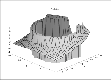
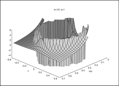
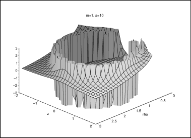
Figure 3: Plots of $V_{\rm eff}$, for $m=a=1$, $m=10a=10$, and $a=10m=10$.

Before staring the discussion on quantum theory, let us have another look to the original Lagrangian (93). We mention that the Lagrangian is in the form of a pure kinetic term, represented by means of a metric $g_{ij}(x)$ as

$$L=\frac{1}{2}\frac{m}{2}g_{ij}(x)\;\dot{x}^{i}\dot{x}^{j},$$ (98)

in which $x^{i}=(\rho,\phi,z)$, and

$$g_{11}(\rho,z)=1+af_{1}(r), \;\;\;\;g_{22}(\rho,z)=\rho^{2}\big{[}1+a\big{(}f_{1}(r)-\rho^{2}f_{2}(r)\big{)}\big{]},$$

$$g_{33}=1, \;\;\;\;\;\;g_{ij}=0,\;\;i\neq j.$$ (99)

We remind that although the Lagrangian is looking like a pure kinetic term, since one of the components of metric, $g_{22}$, changes sign, we can have negative energy states, among them there are bound states. By this interpretation of Lagrangian, the Hamiltonian of quantum theory is simply gained:

$$H_{\rm 2b}=-\frac{1}{m}\nabla^{2}=-\frac{1}{m}\frac{1}{\sqrt{|\det g|}}\partial_{i}\Big{[}\sqrt{|\det g|}\;g^{ij}\;\partial_{j}\Big{]}$$ (100)

in which $\deg g$ is the determinant of $g_{ij}$. As $g_{ij}$ is diagonal, $g^{ij}=1/g_{ij}$, for non-zero $g^{ij}$’s. We mention $\deg g$ and components of $g^{ij}$ are independent of coordinate $\phi$, and so we find

$$H_{\rm 2b}=-\frac{1}{m}\bigg{\{}\frac{1}{\sqrt{g_{11}|g_{22}|}}\partial_{\rho}\Big{[}\sqrt{\frac{|g_{22}|}{g_{11}}}\;\partial_{\rho}\Big{]}+\frac{1}{\sqrt{g_{11}|g_{22}|}}\partial_{z}\Big{[}\sqrt{g_{11}|g_{22}|}\;\partial_{z}\Big{]}+\frac{1}{g_{22}}\partial_{\phi}^{2}\bigg{\}}$$ (101)

Using the separation of variables, we choose the wave-function $\Psi(\rho,z,\phi)=\psi(\rho,z)\Phi(\phi)$, with $\Phi(\phi)\propto{\rm e}^{il\phi}$, and due to single valued-ness of wave-function, $l$ should be an integer. So we replace $\frac{1}{g_{22}}\partial_{\phi}^{2}$ by $-\frac{l^{2}}{g_{22}}$ in above, getting

$$H_{\rm 2b}^{l}=-\frac{1}{m}\bigg{\{}\frac{1}{\sqrt{g_{11}|g_{22}|}}\partial_{\rho}\Big{[}\sqrt{\frac{|g_{22}|}{g_{11}}}\;\partial_{\rho}\Big{]}+\frac{1}{\sqrt{g_{11}|g_{22}|}}\partial_{z}\Big{[}\sqrt{g_{11}|g_{22}|}\;\partial_{z}\Big{]}-\frac{l^{2}}{g_{22}}\bigg{\}}$$ (102)

in which $H^{l}_{\rm 2b}$ means the Hamiltonian for states with specified value for $l$. By comparison, we see that the classical counterpart of integer number $l$ is $K$. Also we mention that $l^{2}/(mg_{22})$, as expected, is sitting for $V_{\rm eff}$ in quantum theory. Now let us choose a trial-function $f(\rho,z)$, that vanishes outside the curve $g(\rho,z)=0$. We consider the quantity:

$$\big{\langle}f\big{|}H^{l}_{\rm 2b}\big{|}f\big{\rangle} = \int_{{\rm inside}\;g(\rho,z)=0}f^{*}(\rho,z)\Big{(}H^{l}_{\rm 2b}f(\rho,z)\Big{)}\sqrt{|\det g|}\,{\rm d}\rho\,{\rm d}z$$ (103)

$$= A_{1,f}-l^{2}A_{2,f}=:E_{f,l}$$

in which $A_{1,f}$ and $A_{2,f}$ are two numbers independent of $l$. We mention that, since $f(\rho,z)$ vanishes in $r\to\infty$, the contribution coming from the first two terms of $H^{l}_{\rm 2b}$, taking into account the minus sign in front, is positive. The contribution from the last term of $H^{l}_{\rm 2b}$, reminding the definition of $f(\rho,z)$, is negative. So for this kind of trial-function, $A_{1,f}$ and $A_{2,f}$ are positive. Here we make comment on the existence of bound states, at least for some ranges of $l$. We mention that for sufficiently large values of $l$, for a fixed trial-function $f(\rho,z)$, $E_{f,l}$ can be negative. In fact one can, by increasing $l$, lower $E_{f,l}$ as much as wants. Now, by variational theorem we know that $E_{f,l}$ is an upper limit for the lowest energy, and so we expect that for states with sufficient large $l$, there should be negative eigenvalues for Hamiltonian $H^{l}_{\rm 2b}$. Showing these negative eigenvalues by $E_{n,l}$, and the corresponding eigenfunctions by $\psi_{n,l}(\rho,z)$, with $n$ as for the possible quantum numbers, we have

$$\widetilde{\nabla}^{2}\psi_{n,l}(\rho,z)=\Big{(}\frac{l^{2}}{g_{22}}-mE_{n,l}\Big{)}\psi_{n,l}(\rho,z)$$ (104)

with $\widetilde{\nabla}^{2}$ as the Laplacian in $\rho z$-plane, given by

$$\widetilde{\nabla}^{2}=\frac{1}{\sqrt{g_{11}|g_{22}|}}\partial_{\rho}\Big{[}\sqrt{\frac{|g_{22}|}{g_{11}}}\;\partial_{\rho}\Big{]}+\frac{1}{\sqrt{g_{11}|g_{22}|}}\partial_{z}\Big{[}\sqrt{g_{11}|g_{22}|}\;\partial_{z}\Big{]}$$ (105)

Now, since outside of the curve $g(\rho,z)=0$ the potential $V_{\rm eff}$ is positive definite, the coefficient of $\psi_{n,l}$ in the right-hand-side is also positive. As $r\to\infty$ belongs to the outside of the curve $g(\rho,z)=0$, by the properties of spectrum of $\widetilde{\nabla}^{2}$, we expect $\psi_{n,l}|_{r\to\infty}\to 0$, that is $\psi_{n,l}$ is representing a bound state. Physically we expect that for the negative eigenvalues, the wave-function should be localized along the well inside the curve $g(\rho,z)=0$, as $g_{22}$ approaching zero from below.

The manner we approved the existence of bound states can be used, by increasing $l$, for reasoning that there is no lowest energy state: the eigenvalues are unbounded from below. We recall that the potential (85) is obtained under the assumption that $\lambda\ll r$. As $\bm{\lambda}=\frac{1}{2}\;\mathbf{p}\times\bm{\theta}$, we see that for large values of momentum, $\lambda$ may be comparable, and even bigger than $r$. One situation that might invalidate the assumption $\lambda\ll r$ can happen for very large values of $l$, corresponding to large value of $K$ in classical theory. In such cases one should consider the original potential (80). We remind that, although the absolute least energy is meaningless to be found under the approximation $\lambda\ll r$, the least value of energy is still meaningful for states with specified value for $l$.

The other issue is about states with eigenvalues bigger than the maximum of potential inside the curve $g(\rho,z)=0$. We mention that an infinite tall wall has surrounded the inside region, and the question is if the wall can make the possibility for forming bound states. In fact since the thickness of wall behaves like $1/h$, with $h$ as height, by considerations coming from the WKB approximation for tunnelling effect, we expect that the particles with positive energies can escape from the inside region. This situation is similar to the situation in one dimensional problem with potential $V(x)=1/(x-x_{0})$, for which by WKB method one finds a finite probability expression for tunnelling of positive energy particles.

As the final point, we make comment on the possible values of spin and $l$. The state of a two-photon system should be symmetric under the exchange of photons. A two-photon system can have 0, 1 and 2 as total spins, as for the first and last ones the spin states are symmetric, and for the second is anti-symmetric. Here the exchange of two photons means $z\to-z$ and $\phi\to\phi+\pi$. By considering the spatial dependence of wave-function, we have the followings for allowed spins and $l$:

$$S=0,2, l=0,2,4,\cdots$$

$$S=1, l=1,3,5,\cdots$$ (106)

5 Conclusion And Discussion

We mention that the transformations of gauge field as well as the field strength in a noncommutative space look like to those of non-Abelian gauge theories. Besides we see that the action of noncommutative QED contains terms which are responsible for interaction between photons, again as the situation we have in non-Abelian gauge theories. There is another observation that promotes the formal similarities of noncommutative and non-Abelian theories to their behaviors, that is the negative sign of $\beta$-function, which manifests that these theories are asymptotically free [13, 14]. The above mentioned observations make it reasonable to study whether and how the photons of noncommutative QED can make bound states. Also these observations make it reasonable to see if the techniques developed for QCD purposes can also be used for noncommutative QED. Here we used the so-called potential model, developed on the constituent gluon picture of QCD glue-balls. The basic ingredient of potential model is that the self-interacting massless gauge particles may get mass by inclusion non-perturbative effects. By calculating the amplitude for the scattering process between two massive photons, we extract the effective potential that is expected capture the dynamics of constituent photons. Using this effective potential, we formulate the Hamiltonian dynamics, by which arguments are presented in favor of existence of photon bound states.

As possible photo-balls, like their glue-ball cousins, are non-perturbative in nature, it is expected that lattice version of noncommutative QED should appear as one of the natural ways to study photo-ball’s properties. It is remarkable to remind that ordinary QED on lattice develops an area law, suggesting a stringy picture for force, for two charged particles [27]. There are suggestions for lattice version of noncommutative gauge theories [28]. Specially, the finite $N$ version of the theory is promising for numerical and simulation purposes. Recently, there have been a few works reporting the preliminaries results by the lattice version of theories [29]. There are other suggestions for non-perturbative definition of noncommutative QED [30].

By the current experiments there has not been any signal for possible noncommutativity. So the common expectation is that the evidence for noncommutativity, if any, should modifies the processes that occur in energies much higher than those presently available. It is why that by present experimental data one can just suggest an upper limit for noncommutative effects. There has been another suggestion that the noncommutativity effects may appear due to applying sufficiently strong magnetic field on samples containing moving charged particles. It would be extremely interesting if noncommutative view let us know something new about relevant phenomena [31].

Acknowledgement: A. H. F. is grateful to M. Khorrami for very helpful discussions on the distributional derivatives, and also for extremely useful discussions on the bound state problem.

Appendix A Distributional Derivatives

Here we calculate the distributional derivatives. One very helpful reference is [26]. First we consider

$$\partial_{i}\partial_{j}\frac{{\rm e}^{-mr}}{r}$$ (107)

The distributional derivative can be calculated by its effect on a test-function $\phi(\mathbf{r})$

$$\Big{\langle}\partial_{i}\partial_{j}\frac{{\rm e}^{-mr}}{r},\phi\Big{\rangle} := \Big{\langle}\frac{{\rm e}^{-mr}}{r},\partial_{i}\partial_{j}\phi\Big{\rangle}=\!\int\frac{{\rm e}^{-mr}}{r}\;\partial_{i}\partial_{j}\phi(\mathbf{r}){\rm d}^{3}\!\!\;r$$ (108)

$$= \!\!\!\!\lim_{\varepsilon\to 0^{+}}\int_{r\geq\varepsilon}\!\!\!\frac{{\rm e}^{-mr}}{r}\;\partial_{i}\partial_{j}\phi(\mathbf{r}){\rm d}^{3}\!\!\;r$$

in which ${\rm d}^{3}\!\!\;r=r^{2}{\rm d}r{\rm d}\Omega$. The limit above does exist because the integral in the second line, due to $r^{2}$ in ${\rm d}^{3}\!\!\;r$, is finite. $r=0$ is excluded from the last integral, and so we can use the identity

$$\frac{{\rm e}^{-mr}}{r}\partial_{i}\partial_{j}\phi=\partial_{i}\Big{(}\frac{{\rm e}^{-mr}}{r}\partial_{j}\phi\Big{)}-\partial_{i}\frac{{\rm e}^{-mr}}{r}\;\;\partial_{j}\phi$$ (109)

by which we have for $I_{ij}=\Big{\langle}\partial_{i}\partial_{j}\frac{{\rm e}^{-mr}}{r},\phi\Big{\rangle}$

$$I_{ij} = \lim_{\varepsilon\to 0^{+}}\bigg{[}\int_{r\geq\varepsilon}\partial_{i}\Big{(}\frac{{\rm e}^{-mr}}{r}\partial_{j}\phi\Big{)}{\rm d}^{3}\!\!\;r\!-\int_{r\geq\varepsilon}\partial_{i}\frac{{\rm e}^{-mr}}{r}\;\partial_{j}\phi\,{\rm d}^{3}\!\!\;r\bigg{]}$$ (110)

$$= \lim_{\varepsilon\to 0^{+}}\bigg{[}\int_{r\geq\varepsilon}\bm{\nabla}\cdot\Big{(}{\mathbf{\hat{e}}}_{i}\frac{{\rm e}^{-mr}}{r}\partial_{j}\phi\Big{)}{\rm d}^{3}\!\!\;r\!-\int_{r\geq\varepsilon}\partial_{i}\frac{{\rm e}^{-mr}}{r}\partial_{j}\phi\,{\rm d}^{3}\!\!\;r\bigg{]}$$

$$= \lim_{\varepsilon\to 0^{+}}\bigg{[}\!\int_{r=\varepsilon}\frac{{\rm e}^{-mr}}{r}\partial_{j}\phi(-{\mathbf{\hat{e}}}_{i}\cdot{\mathbf{\hat{r}}})r^{2}{\rm d}\Omega-\int_{r\geq\varepsilon}\partial_{i}\frac{{\rm e}^{-mr}}{r}\partial_{j}\phi\,{\rm d}^{3}\!\!\;r\bigg{]}$$

$$= \lim_{\varepsilon\to 0^{+}}\bigg{[}-\int_{r=\varepsilon}\frac{{\rm e}^{-mr}}{r}\partial_{j}\phi\;n_{i}r^{2}{\rm d}\Omega-\int_{r\geq\varepsilon}\partial_{i}\frac{{\rm e}^{-mr}}{r}\partial_{j}\phi\,{\rm d}^{3}\!\!\;r\bigg{]}$$

in which ${\mathbf{\hat{e}}}_{i}$ is for unit vector in $x$, $y$ and $z$ directions, and ${\mathbf{\hat{r}}}=(n_{1},n_{2},n_{3})$. The first integral in last line is proportional to $\varepsilon$ and so vanishes in the limit. So we get

$$I_{ij}=-\lim_{\varepsilon\to 0^{+}}\int_{r\geq\varepsilon}\!\partial_{i}\frac{{\rm e}^{-mr}}{r}\;\partial_{j}\phi\;{\rm d}^{3}\!\!\;r$$ (111)

By repeating the steps above, we arrive at:

$$I_{ij} = \lim_{\varepsilon\to 0^{+}}\bigg{[}\int_{r=\varepsilon}\phi\,\partial_{i}\frac{{\rm e}^{-mr}}{r}\;n_{j}r^{2}{\rm d}\Omega+\int_{r\geq\varepsilon}\phi\,\partial_{i}\partial_{j}\frac{{\rm e}^{-mr}}{r}\,{\rm d}^{3}\!\!\;r\bigg{]}$$ (112)

$$= \lim_{\varepsilon\to 0^{+}}\bigg{[}-\phi(\varepsilon)\int n_{i}n_{j}{\rm d}\Omega+\int_{r\geq\varepsilon}\phi\,\partial_{i}\partial_{j}\frac{{\rm e}^{-mr}}{r}\,{\rm d}^{3}\!\!\;r\bigg{]}$$

for getting it we used $\partial_{i}f(r)=n_{i}\partial_{r}f(r)$, and also keeping the integrand of first integral to the first non-vanishing order in $\varepsilon$. We know

$$\int n_{i}n_{j}{\rm d}\Omega=A_{2}\delta_{ij}$$ (113)

and $A_{2}$ can be calculated by taking trace of the both sides, yielding $A_{2}=\frac{4\pi}{3}$. By these all we have

$$I_{ij}=-\frac{4\pi}{3}\phi(0)\delta_{ij}+\lim_{\varepsilon\to 0^{+}}\!\int_{r\geq\varepsilon}\!\!\!\phi\;\partial_{i}\partial_{j}\frac{{\rm e}^{-mr}}{r}\,{\rm d}^{3}\!\!\;r$$ (114)

The limit above exists, by using the fact that the value of function in origin is constant and independent from the $\Omega=\Omega(\theta,\varphi)$, and recalling

$$\int(3n_{i}n_{j}-\delta_{ij}){\rm d}\Omega=0$$ (115)

One can remove the limit by respecting the order of integrations. By these all we get

$$\partial_{i}\partial_{j}\frac{{\rm e}^{-mr}}{r}\to-\frac{4\pi}{3}\delta_{ij}\delta(\mathbf{r})+{\rm pf}\Big{[}\partial_{i}\partial_{j}\frac{{\rm e}^{-mr}}{r}\Big{]}$$ (116)

in which “ pf ” is sitting for pseudo-function, that here simply means that in integrals the integration on solid-angle should be done before radial one.

Now we come to

$$I_{ijk} = \Big{\langle}\partial_{i}\partial_{j}\partial_{k}\frac{{\rm e}^{-mr}}{r},\phi\Big{\rangle}:=-\Big{\langle}\frac{{\rm e}^{-mr}}{r},\partial_{i}\partial_{j}\partial_{k}\phi\Big{\rangle}$$ (117)

$$= \!\!-\int\frac{{\rm e}^{-mr}}{r}\;\partial_{i}\partial_{j}\partial_{k}\phi(\mathbf{r}){\rm d}^{3}\!\!\;r$$

$$= \!\!-\lim_{\varepsilon\to 0^{+}}\int_{r\geq\varepsilon}\!\!\!\frac{{\rm e}^{-mr}}{r}\;\partial_{i}\partial_{j}\partial_{k}\phi(\mathbf{r}){\rm d}^{3}\!\!\;r$$

in which again the limit exists because the integral in the second line is finite. By repeating the steps for calculation $I_{ij}$, and the replacement

$$\phi(\varepsilon)=\phi(0)+\varepsilon\,{\mathbf{\hat{r}}}\cdot\bm{\nabla}\phi(0)+O(\varepsilon^{2})$$ (118)

and using

$$\int n_{i}n_{j}n_{k}n_{p}{\rm d}\Omega=A_{4}\big{[}\delta_{ij}\delta_{kp}+\delta_{ik}\delta_{jp}+\delta_{ip}\delta_{jk}\big{]}$$

$$\int n_{i}{\rm d}\Omega=\int n_{i}n_{j}n_{k}{\rm d}\Omega=0,$$ (119)

with $A_{4}=\frac{4\pi}{15}$, one reaches to

$$I_{ijk} = \frac{4\pi}{5}\Big{[}\delta_{ij}\partial_{k}\phi(0)+\delta_{jk}\partial_{i}\phi(0)+\delta_{ki}\partial_{j}\phi(0)\Big{]}+\lim_{\varepsilon\to 0^{+}}\!\int_{r\geq\varepsilon}\!\!\!\phi\;\partial_{i}\partial_{j}\partial_{k}\frac{{\rm e}^{-mr}}{r}\,{\rm d}^{3}\!\!\;r$$ (120)

for which again the limit above exists while one is careful that the integration on ${\rm d}\Omega$ should be done firstly. By these all we get

$$\partial_{i}\partial_{j}\partial_{k}\frac{{\rm e}^{-mr}}{r} \to -\frac{4\pi}{5}\Big{[}\delta_{ij}\partial_{k}+\delta_{jk}\partial_{i}+\delta_{ki}\partial_{j}\Big{]}\delta(\mathbf{r})+\;{\rm pf}\Big{[}\partial_{i}\partial_{j}\partial_{k}\frac{{\rm e}^{-mr}}{r}\Big{]}$$ (121)

in which again “ pf ” simply means in integrals the integration on solid-angle should be done before radial one.

Now we come to

$$I_{ijkl} = \Big{\langle}\partial_{i}\partial_{j}\partial_{k}\partial_{l}\frac{{\rm e}^{-mr}}{r},\phi\Big{\rangle}:=\Big{\langle}\frac{{\rm e}^{-mr}}{r},\partial_{i}\partial_{j}\partial_{k}\partial_{l}\phi\Big{\rangle}$$ (122)

$$= \!\!\int\frac{{\rm e}^{-mr}}{r}\;\partial_{i}\partial_{j}\partial_{k}\partial_{l}\phi(\mathbf{r}){\rm d}^{3}\!\!\;r$$

$$= \!\!\lim_{\varepsilon\to 0^{+}}\int_{r\geq\varepsilon}\!\!\!\frac{{\rm e}^{-mr}}{r}\;\partial_{i}\partial_{j}\partial_{k}\partial_{l}\phi(\mathbf{r}){\rm d}^{3}\!\!\;r$$

in which again the limit exists because the integral in the second line is finite. By repeating the steps for calculation $I_{ij}$ and $I_{ijk}$, and the replacement

$$\phi(\varepsilon)=\phi(0)+\varepsilon\,{\mathbf{\hat{r}}}\cdot\bm{\nabla}\phi(0)+\frac{\varepsilon^{2}}{2}({\mathbf{\hat{r}}}\cdot\bm{\nabla})^{2}\phi(0)+O(\varepsilon^{3})$$ (123)

and using

$$\int n_{i}n_{j}n_{k}n_{p}n_{q}{\rm d}\Omega = 0$$

$$\int n_{i}n_{j}n_{k}n_{l}n_{p}n_{q}{\rm d}\Omega = A_{6}\big{[}\delta_{ij}\delta_{kl}\delta_{pq}+\delta_{ik}\delta_{jl}\delta_{pq}+\delta_{il}\delta_{kj}\delta_{pq}$$ (124)

$$\quad+\delta_{ij}\delta_{kp}\delta_{lq}+\delta_{ij}\delta_{kq}\delta_{lp}+\delta_{ik}\delta_{jp}\delta_{lq}$$

$$\quad+\delta_{ik}\delta_{jq}\delta_{lp}+\delta_{il}\delta_{kp}\delta_{jq}+\delta_{il}\delta_{kq}\delta_{jp}$$

$$\quad+\delta_{ip}\delta_{kl}\delta_{jq}+\delta_{ip}\delta_{kj}\delta_{lq}+\delta_{ip}\delta_{kq}\delta_{jl}$$

$$\quad+\delta_{iq}\delta_{kl}\delta_{jp}+\delta_{iq}\delta_{kj}\delta_{lp}+\delta_{iq}\delta_{kp}\delta_{jl}\big{]}$$

with $A_{6}=\frac{4\pi}{17\times 9}$, one reaches to

$$I_{ijkl} = -\frac{4\pi}{15}\Big{[}\delta_{ij}\delta_{kl}+\delta_{ik}\delta_{jl}+\delta_{il}\delta_{jk}\Big{]}\phi(0)-\frac{10\pi}{51}\Big{[}\delta_{ij}\delta_{kl}+\delta_{ik}\delta_{jl}+\delta_{il}\delta_{jk}\Big{]}\nabla^{2}\phi(0)$$ (125)

$$-\frac{20\pi}{51}\Big{[}\delta_{ij}\partial_{k}\partial_{l}+\delta_{ik}\partial_{j}\partial_{l}+\delta_{il}\partial_{j}\partial_{k}+\delta_{kl}\partial_{i}\partial_{j}+\delta_{jl}\partial_{i}\partial_{k}+\delta_{kj}\partial_{i}\partial_{l}\Big{]}\phi(0)$$

$$+\lim_{\varepsilon\to 0^{+}}\!\int_{r\geq\varepsilon}\!\!\!\phi\;\partial_{i}\partial_{j}\partial_{k}\partial_{l}\frac{{\rm e}^{-mr}}{r}\,{\rm d}^{3}\!\!\;r$$

for which again the limit above exists while one is careful that the integration on ${\rm d}\Omega$ should be done firstly. By these all we get

$$\partial_{i}\partial_{j}\partial_{k}\partial_{l}\frac{{\rm e}^{-mr}}{r} \to -\frac{4\pi}{15}\Big{[}\delta_{ij}\delta_{kl}+\delta_{ik}\delta_{jl}+\delta_{il}\delta_{jk}\Big{]}\delta(\mathbf{r})-\frac{10\pi}{51}\Big{[}\delta_{ij}\delta_{kl}+\delta_{ik}\delta_{jl}+\delta_{il}\delta_{jk}\Big{]}\nabla^{2}\delta(\mathbf{r})$$ (126)

$$-\frac{20\pi}{51}\Big{[}\delta_{ij}\partial_{k}\partial_{l}+\delta_{ik}\partial_{j}\partial_{l}+\delta_{il}\partial_{j}\partial_{k}+\delta_{kl}\partial_{i}\partial_{j}+\delta_{jl}\partial_{i}\partial_{k}+\delta_{kj}\partial_{i}\partial_{l}\Big{]}\delta(\mathbf{r})$$

$$+{\rm pf}\Big{[}\partial_{i}\partial_{j}\partial_{k}\partial_{l}\frac{{\rm e}^{-mr}}{r}\Big{]}$$

in which again “ pf ” simply means in integrals the integration on solid-angle should be done before radial one. The combination $\nabla^{2}\partial_{i}\partial_{j}$ is simply $\delta^{kl}\partial_{i}\partial_{j}\partial_{k}\partial_{l}$.

References

- [1] J. M. Cornwall, “Quark Confinement And Vortices In Massive Gauge-Invariant QCD,” Nucl. Phys. B157 (1979) 392.
- [2] J. M. Cornwall, “Dynamical Mass Generation In Continuum Quantum Chromodynamics,” Phys. Rev. D26 (1982) 1453.
- [3] J. M. Cornwall and A. Soni, “Glueballs As Bound States Of Massive Gluons,” Phys. Lett. B120 (1983) 431.
- [4] W.-S. Hou, C.-S. Luo and G.-G. Wong, “Glueball States In A Constituent Gluon Model,” Phys. Rev. D64 (2001) 014028, hep-ph/0101146.
- [5] W.-S. Hou and G.-G. Wong, “Glueball Spectrum From A Potential Model,” Phys. Rev. D67 (2003) 034003, hep-ph/0207292.
- [6] H. S. Snyder, “Quantized Space-Time,” Phys. Rev. 71 (1947) 38; “The Electromagnetic Field In Quantized Space-Time,” Phys. Rev. 72 (1947) 68.
- [7] E. Witten, “Bound States Of Strings And -Branes,” Nucl. Phys. B460 (1996) 335, hep-th/9510135.
- [8] N. Seiberg and E. Witten, “String Theory And Noncommutative Geometry,” J. High Energy Phys. 9909 (1999) 032, hep-th/9908142.
- [9] A. Connes, M. R. Douglas and A. Schwarz, “Noncommutative Geometry And Matrix Theory: Compactification On Tori,” J. High Energy Phys. 9802 (1998) 003, hep-th/9711162; M. R. Douglas and C. Hull, “D-Branes And The Noncommutative Torus,” J. High Energy Phys. 9802 (1998) 008, hep-th/9711165.
- [10] H. Arfaei and M. M. Sheikh-Jabbari, “Mixed Boundary Conditions And Brane-String Bound States,” Nucl. Phys. B526 (1998) 278, hep-th/9709054.
- [11] M. R. Douglas and N. A. Nekrasov, “Noncommutative Field Theory,” Rev. Mod. Phys. 73 (2001) 977, hep-th/0106048.
- [12] A. H. Fatollahi, “Gauge Symmetry As Symmetry Of Matrix Coordinates,” Eur. Phys. J. C17 (2000) 535, hep-th/0007023; “On Non-Abelian Structure From Matrix Coordinates,” Phys. Lett. B512 (2001) 161, hep-th/0103262; “Electrodynamics On Matrix Space: Non-Abelian By Coordinates,” Eur. Phys. J. C21 (Jul. 2001) 717, hep-th/0104210.
- [13] C. P. Martin and D. S. Sanchez-Ruiz, “The One-Loop UV Divergent Structure Of U(1) Yang-Mills Theory On Noncommutative ,” Phys. Rev. Lett. 83 (1999) 476, hep-th/9903077.
- [14] M. M. Sheikh-Jabbari, “One Loop Renormalizability Of Supersymmetric Yang-Mills Theories On Noncommutative Two-Torus,” J. High Energy Phys. 9906 (1999) 015, hep-th/9903107.
- [15] H. Arfaei and M. H. Yavartanoo, “Phenomenological Consequences Of Noncommutative QED,” hep-th/0010244; J. L. Hewett, F. J. Petriello, and T. G. Rizzo, “Signals For Noncommutative Interactions At Linear Colliders,” Phys. Rev. D64 (2001) 075012, hep-ph/0010354; P. Mathews, “Compton Scattering In Noncommutative Space-Time At The NLC,” Phys. Rev. D63 (2001) 075007, hep-ph/0011332; S.-W. Baek, D. K. Ghosh, X.-G. He, and W. Y. P. Hwang, “Signatures Of Noncommutative QED At Photon Colliders,” Phys. Rev. D64 (2001) 056001, hep-ph/0103068; T. M. Aliev, O. Ozcan, and M. Savci, “The Decay In Noncommutative Quantum Electrodynamics,” Eur. Phys. J. C27 (2003) 447, hep-ph/0209205; H. Grosse and Y. Liao, “Pair Production Of Neutral Higgs Bosons Through Noncommutative QED Interactions At Linear Colliders,” Phys. Rev. D64 (2001) 115007, hep-ph/0105090.
- [16] M. Chaichian, M. M. Sheikh-Jabbari, and A. Tureanu, “Hydrogen Atom Spectrum And The Lamb Shift In Noncommutative QED,” Phys. Rev. Lett. 86 (2001) 2716, hep-th/0010175; “Comments On The Hydrogen Atom Spectrum In The Noncommutative Space,” Eur. Phys. J. C36 (2004) 251, hep-th/0212259.
- [17] N. Chair and M. M. Sheikh-Jabbari, “Pair Production By A Constant External Field In Noncommutative QED,” Phys. Lett. B504 (2001) 141, hep-th/0009037; M. Haghighat, S. M. Zebarjad, and F. Loran, “Positronium Hyperfine Splitting In Noncommutative Space At The Order ,” Phys. Rev. D66 (2002) 016005, hep-ph/0109105; M. Haghighat and F. Loran, “Helium Atom Spectrum In Non-Commutative Space,” Phys. Rev. D67 (2003) 096003, hep-th/0206019; M. Caravati, A. Devoto, and W. W. Repko, “Noncommutative QED And The Lifetimes Of Ortho And Para Positronium,” Phys. Lett. B556 (2003) 123, hep-ph/0211463.
- [18] I. F. Riad and M. M. Sheikh-Jabbari, “Noncommutative QED And Anomalous Dipole Moments,” J. High Energy Phys. 0008 (2000) 045, hep-th/0008132.
- [19] N. Mahajan, “Noncommutative QED And Gamma Gamma Scattering,” hep-ph/0110148.
- [20] G. Berrino, S. L. Cacciatori, A. Celi, L. Martucci, and A. Vicini, “Noncommutative Electrodynamics,” Phys. Rev. D67 (2003) 065021, hep-th/0210171; C. A. de S. Pires, “Photon Deflection By A Coulomb Field In Noncommutative QED,” J. Phys. G30 (2004) B41, hep-ph/0410120; S. M. Lietti and C. A. de S. Pires, “Testing Non Commutative QED And Couplings At LHC,” Eur. Phys. J. C35 (2004) 137, hep-ph/0402034; T. Mariz, C. A. de S. Pires, and R. F. Ribeiro, “Ward Identity In Noncommutative QED,” Int. J. Mod. Phys. A18 (2003) 5433, hep-ph/0211416; S. I. Kruglov, “Maxwell’s Theory On Non-Commutative Spaces And Quaternions,” Annales Fond. Broglie 27 (2002) 343, hep-th/0110059; “Dirac’s Quantization Of Maxwell’s Theory On Non-Commutative Spaces,” Electromagn. Phenom. 3 (2003) 18, quant-ph/0204137; “Generalized Maxwell Equations And Their Solutions,” Annales Fond. Broglie 26 (2001) 125, math-ph/0110008.
- [21] D. V. Vassilevich and A. Yurov, “Space-Time Non-Commutativity Tends To Create Bound States,” Phys. Rev. D69 (2004) 105006, hep-th/0311214.
- [22] K. Dasgupta and M. M. Sheikh-Jabbari, “Noncommutative Dipole Field Theories,” J. High Energy Phys. 0202 (2002) 002, hep-th/0112064.
- [23] M. M. Sheikh-Jabbari, “Open Strings In A B-Field Background As Electric Dipoles,” Phys. Lett. B455 (1999) 129, hep-th/9901080; A. Mazumdar and M. M. Sheikh-Jabbari, “Noncommutativity In Space And Primordial Magnetic Field,” Phys. Rev. Lett. 87 (2001) 011301, hep-ph/0012363.
- [24] A. H. Fatollahi and H. Mohammadzadeh, “On The Classical Dynamics Of Charges In Noncommutative QED,” Eur. Phys. J. C36 (2004) 113, hep-th/0404209.
- [25] H. Goldstein, “Classical Mechanics,” Addison-Wesley, 2nd ed., p. 352.
- [26] I. Stakgold, “Green’s Functions And Boundary Value Problems,” John Wiley & Sons, ch. 2, 1998.
- [27] K. G. Wilson, “Confinement Of Quarks,” Phys. Rev. D10 (1974) 2445.
- [28] J. Ambjørn, Y. M. Makeenko, J. Nishimura, and R. J. Szabo, “Finite N Matrix Models Of Noncommutative Gauge Theory,” J. High Energy Phys. 9911 (1999) 029, hep-th/9911041; “ Nonperturbative Dynamics Of Noncommutative Gauge Theory,” Phys. Lett. B480 (2000) 399, hep-th/0002158; “Lattice Gauge Fields And Discrete Noncommutative Yang-Mills Theory,” J. High Energy Phys. 0005 (2000) 023, hep-th/0004147.
- [29] W. Bietenholz, F. Hofheinz and J. Nishimura, “A Non-Perturbative Study of Gauge Theory On A Non-Commutative Plane,” J. High Energy Phys. 0209 (2002) 009, hep-th/0203151; W. Bietenholz, F. Hofheinz, J. Nishimura, Y. Susaki, and J. Volkholz, “First Simulation Results For The Photon In A Non-Commutative Space,” hep-lat/0409059; W. Bietenholz, A. Bigarini, F. Hofheinz, J. Nishimura, Y. Susaki, and J. Volkholz, “Numerical Results For U(1) Gauge Theory On 2d And 4d Non-Commutative Spaces,” hep-th/0501147.
- [30] H. Grosse and H. Steinacker, “Finite Gauge Theory On Fuzzy CP2,” Nucl. Phys. B707 (2005) 145, hep-th/0407089; W. Behr, F. Meyer, and H. Steinacker, “Gauge Theory On Fuzzy SS2 And Regularization On Noncommutative ,” hep-th/0503041.
- [31] Z. Guralnik, R. Jackiw, S. Y. Pi, and A. P. Polychronakos, “Testing Non-Commutative QED, Constructing Non-Commutative MHD,” Phys. Lett. B517 (2001) 450, hep-th/0106044; R. Jackiw, “Physical Instances of Noncommuting Coordinates,” Nucl. Phys. Proc. Suppl. 108 (2002) 30, hep-th/0110057.