hep-th/0503068

MIT-CTP-3606

Vacuum string field theory without matter-ghost factorization
Nadav Drukker¹ and Yuji Okawa^2
1 The Niels Bohr Institute, Copenhagen University
Blegdamsvej 17, DK-2100 Copenhagen, Denmark
drukker@nbi.dk
² Center for Theoretical Physics, Room 6-304
Massachusetts Institute of Technology
Cambridge, MA 02139, USA
okawa@lns.mit.edu
Abstract

We show that vacuum string field theory with the singular kinetic operator conjectured by Gaiotto, Rastelli, Sen and Zwiebach can be obtained by field redefinition from a regular theory constructed by Takahashi and Tanimoto. We solve the equation of motion both by level truncation and by a series expansion using the regulated butterfly state, and we find evidence that the energy density of a D25-brane is well defined and finite. Although the equation of motion naively factorizes into the matter and ghost sectors in the singular limit, subleading terms in the kinetic operator are relevant and the factorization does not strictly hold. Nevertheless, solutions corresponding to different D-branes can be constructed by changing the boundary condition in the boundary conformal field theory formulation of string field theory, and ratios of D-brane tensions are shown to be reproduced correctly.

1 Introduction

Vacuum string field theory [1, 2, 3] is a conjectured form of Witten’s cubic open string field theory [4] expanded around the tachyon vacuum. The action of vacuum string field theory is given by replacing the BRST operator in Witten’s string field theory with a different operator which we denote by ${\cal Q}$. It was conjectured in [1] that this operator can be made purely of ghost fields, and under this assumption the equation of motion factorizes into the matter and ghost sectors. Then the matter part of the equation can be solved by the matter sector of a star-algebra projector [2, 6] such as the sliver state [7, 8] or the butterfly state [9, 10, 11, 12]. Using the conformal field theory (CFT) formulation of string field theory [13, 14], we can construct such a star-algebra projector for any given consistent open-string boundary condition [7]. The resulting solution is conjectured to describe the D-brane corresponding to the open-string boundary condition [7, 15]. Based on this description of D-branes, it has been shown that ratios of D-brane tensions [7, 16], the open-string mass spectrum on any D-brane [17], and the absolute value of the D25-brane tension [17] can be reproduced correctly. The factorization into the matter and ghost sectors is a key ingredient in deriving these results.

A more specific conjecture on the operator ${\cal Q}$ was put forward later by Gaiotto, Rastelli, Sen and Zwiebach [9]. It was conjectured that the kinetic operator is given by a singular limit where ${\cal Q}$ becomes a $c$-ghost insertion at the open-string midpoint with a divergent coefficient. With this kinetic operator, the full equation of motion including the ghost sector can be solved by a star-algebra projector in the twisted CFT [18, 9] or by an ordinary star-algebra projector with an appropriate $c$-ghost insertion [19].

There are, however, remaining problems. It was shown in [12, 19] that when the solution $\left|\Psi\right\rangle$ is given by the twisted butterfly state or by the butterfly state with a $c$-ghost insertion, the equation of motion contracted with the solution $\left|\Psi\right\rangle$,

$$\langle\Psi|{\cal Q}|\Psi\rangle+\langle\Psi|\Psi\ast\Psi\rangle=0\,,$$ (1.1)

turns out to be incompatible with the equation contracted with a state $\left|\phi\right\rangle$ in the Fock space:

$$\langle\phi|{\cal Q}|\Psi\rangle+\langle\phi|\Psi\ast\Psi\rangle=0\,.$$ (1.2)

This follows from the fact that the ratio

$$\frac{\langle\phi|\Psi\ast\Psi\rangle}{\langle\phi|{\cal Q}|\Psi\rangle}\frac{\langle\Psi|{\cal Q}|\Psi\rangle}{\langle\Psi|\Psi\ast\Psi\rangle}$$ (1.3)

is different from $1$ in the limit where ${\cal Q}$ becomes the $c$-ghost insertion at the open-string midpoint. Since this ratio is independent of the normalizations of ${\cal Q}$, $\left|\Psi\right\rangle$, and $\left|\phi\right\rangle$, the conclusion holds whatever scaling limit we may take. One resolution suggested in [12] is the possible relevance of the subleading terms of ${\cal Q}$. Since the solution $\left|\Psi\right\rangle$ is outside the Fock space, the subleading terms in ${\cal Q}$ can contribute to $\langle\phi|{\cal Q}|\Psi\rangle$ or to $\langle\Psi|{\cal Q}|\Psi\rangle$ at the same order as the leading term. In fact, it was demonstrated using an explicit example in [12] that this is indeed possible.

Another issue is the finiteness of the physical coupling constant. Since vacuum string field theory is formulated around a vacuum without physical open string states, the coupling constant in the action is not directly related to physical quantities. The string coupling constant can be read off, for example, from a three-tachyon scattering amplitude around a D25-brane solution as in [17]. The finiteness of the string coupling constant requires the existence of a D-brane solution with finite energy density. In the case of the twisted butterfly state solution, it was shown in [12] that the energy density can be finite in the limit if one appropriately scales the parameter of the solution as the coefficient of the singular pure-ghost kinetic operator diverges. However, whether or not this scaling limit is realized cannot be determined by the analysis at the leading order and depends on the subleading structure of the theory [12]. This also indicates the relevance of the subleading terms in the kinetic operator.

If the subleading terms in ${\cal Q}$ are relevant, the factorization into the matter and ghost sectors at the leading order may be ruined. Since the factorization was a key assumption in deriving the various results mentioned earlier, this could be a serious problem. For example, the construction of other D-brane solutions with correct tension ratios may be no longer valid. Constructing a consistent next-to-leading term in the kinetic operator, however, is a nontrivial problem, which has prevented us from addressing this issue in a specific example.

In this paper, we claim that the assumption of the matter-ghost factorization in the kinetic operator ${\cal Q}$ can be relaxed in constructing D-brane solutions with correct tension ratios. We demonstrate this in a concrete setting based on the regularization of the singular pure-ghost kinetic operator proposed in [20]. We first show in section 2 that vacuum string field theory with the singular kinetic operator conjectured by Gaiotto, Rastelli, Sen and Zwiebach can be realized by field redefinition of a regular theory constructed by Takahashi and Tanimoto [21]. Then in section 3, we solve the equation of motion both by level truncation and by a series expansion using the regulated butterfly state [19], and we find evidence that the energy density of a D25-brane is well defined and finite in this theory. The long-standing issue of the finiteness of the physical coupling constant therefore seems to be resolved in this particular realization of vacuum string field theory with the singular pure-ghost kinetic operator. In this case, however, the subleading terms in the kinetic operator are in fact relevant, and their contributions to physical quantities such as the D25-brane tension are nonvanishing in the singular limit. Therefore, the apparent factorization into the matter and ghost sectors does not strictly hold. Nevertheless, we show in section 4 that solutions corresponding to different D-branes can be constructed by changing the boundary condition in the boundary CFT formulation, and ratios of D-brane tensions can be reproduced correctly. This argument in section 4 is general and is not restricted to this particular choice of the kinetic operator. In fact, we do not even need to assume that the kinetic term can be brought to the singular $c$-ghost insertion at the open-string midpoint. We comment on our results and discuss open problems in section 5.

We use standard conventions in the CFT formulation of string field theory, which are summarized in appendix A. Some details of subsection 3.2 are presented in appendix B.

2 Singular pure-ghost theory from a regular theory

2.1 Singular pure-ghost vacuum string field theory

The action of Witten’s cubic open string field theory [4] is given by

$$S=-\frac{1}{\alpha^{\prime 3}g_{T}^{2}}\left[\frac{1}{2}\langle\Psi|Q_{B}|\Psi\rangle+\frac{1}{3}\langle\Psi|\Psi\ast\Psi\rangle\right],$$ (2.1)

where $g_{T}$ is the on-shell three-tachyon coupling constant. The action of vacuum string field theory is derived from this action by expanding it around the solution corresponding to the tachyon vacuum, and it will take the same form except for the kinetic operator. It was conjectured in [1] that the resulting kinetic operator can be made purely of ghost fields by field redefinition. We write the action of vacuum string field theory as

$$S=-\frac{1}{\alpha^{\prime 3}g^{2}}\left[\frac{1}{2}\langle\Psi|{\cal Q}|\Psi\rangle+\frac{1}{3}\langle\Psi|\Psi\ast\Psi\rangle\right],$$ (2.2)

where we used a different notation $g$ for the coupling constant because the field redefinition may change it from the original value $g_{T}$. We will discuss this point further in subsection 2.3. The equation of motion derived from this action factorizes into the matter and ghost sectors if ${\cal Q}$ can be made purely of ghost fields.

A more specific conjecture on ${\cal Q}$ was put forward later in [9]. It was conjectured that there exists a one-parameter family of field redefinition which takes ${\cal Q}$ to the following form:

$${\cal Q}=\frac{Q}{2\epsilon}\left[1+o(\epsilon)\right]\,,$$ (2.3)

where $Q$ is a midpoint $c$-ghost insertion defined by

$$Q=\frac{1}{2i}(c(i)-c(-i))\,,$$ (2.4)

and $\epsilon$ is the parameter of the field redefinition. We denoted terms which vanish in the limit $\epsilon\to 0$ by $o(\epsilon)$, which does not have to be $O(\epsilon)$. In the singular limit $\epsilon\to 0$, the midpoint $c$-ghost insertion $Q$ dominates in the kinetic operator ${\cal Q}$ with an infinite coefficient.

If there are no subleading terms in (2.3), the parameter $g$ can be absorbed by field redefinition [12]. Therefore, the subleading terms are necessary in order for the theory to have a parameter corresponding to the string coupling constant.

Since vacuum string field theory is formulated around a vacuum where there are no physical open strings, the coupling constant $g$ in the action is not directly related to physical quantities. The physical string coupling constant can be calibrated, for example, by the energy density ${\cal E}$ of a D25-brane. Since ${\cal E}=1/(2\pi^{2}\alpha^{\prime 3}g_{T}^{2})$, $g_{T}$ is given by

$$g_{T}=\frac{1}{\sqrt{2\pi^{2}\alpha^{\prime 3}{\cal E}}}\,.$$ (2.5)

This shows that the energy density of the D25-brane solution in vacuum string field theory should be finite in order to have a finite string coupling constant. It would be less interesting if we only formulated a theory with a vanishing or divergent string coupling constant.

There are other ways to identify the string coupling constant in vacuum string field theory. For example, it can be identified by the on-shell three-tachyon coupling around a D25-brane solution. Strictly speaking, $\alpha^{\prime}$ should also be identified, for example, from the mass spectrum of open strings around a D25-brane. It is a nontrivial check if the energy density of the D25-brane solution can be written as $1/(2\pi^{2}\alpha^{\prime 3}g_{T}^{2})$ with the correct numerical coefficient in terms of $\alpha^{\prime}$ and $g_{T}$ identified in this way. It was shown in [17] that this expression can be in fact reproduced in vacuum string field theory under the assumption of the matter-ghost factorization.

The equation of motion with ${\cal Q}$ given by (2.3) can be solved by a star-algebra projector in the twisted CFT in the limit $\epsilon\to 0$ [9]. It was shown in [12] that the energy density of the solution given by the twisted butterfly state can be finite if one appropriately scales the regularization parameter of the twisted butterfly state in the limit $\epsilon\to 0$. However, whether or not this scaling is realized cannot be determined from the analysis at the leading order, and it depends on the subleading terms [12].

To summarize, the subleading terms in (2.3) are necessary in order for the theory to have a parameter corresponding to the string coupling constant. Furthermore, the finiteness of the physical coupling constant depends on the subleading terms in (2.3).

2.2 Regularizing the singular pure-ghost operator

To address these issues it is therefore important to regularize the singular pure-ghost kinetic operator (2.3). However, it is a nontrivial problem to construct a next-to-leading term in (2.3) which satisfies the conditions for a consistent kinetic operator of string field theory such as ${\cal Q}^{2}=0$. One way to regularize the singular pure-ghost operator was presented in [20] by modifying a class of kinetic operators constructed by Takahashi and Tanimoto [21].

The operators constructed in [21] take the following form:

$$Q_{f}=\oint_{C}\frac{d\xi}{2\pi i}\biggl{[}f(\xi)\,j_{B}(\xi)-\frac{f^{\prime}(\xi)^{2}}{f(\xi)}\,c(\xi)\biggr{]}\,,$$ (2.6)

where $j_{B}(\xi)$ is the BRST current and $f(\xi)$ is any analytic function satisfying $f(-1/\xi)=f(\xi)$. The contour $C$ runs on the unit circle counterclockwise. The operator $Q_{f}$ is formally related to $Q_{B}$ by a similarity transformation so one may expect the theory with $Q_{f}$ to be equivalent to the theory with $Q_{B}$. However, the similarity transformation can be singular, and the theory with $Q_{f}$ can be inequivalent to the theory with $Q_{B}$. The simplest such example considered in [21] is $f(\xi)=-(1-\xi^{2})^{2}/(4\xi^{2})$. It was further required in [21] that $f(\xi)$ is analytic inside the unit disk except for a pole at the origin. However, $Q_{f}$ can be a consistent kinetic operator of string field theory even if $f(\xi)$ has poles away from the origin, and a more general class of operators were discussed in [20]. In particular, if we choose $f(\xi)$ to be

$$f(\xi)=\frac{\epsilon^{2}\left(1-\xi^{2}\right)^{2}}{\epsilon^{2}\left(1-\xi^{2}\right)^{2}-\left(1+\xi^{2}\right)^{2}}\,,$$ (2.7)

$Q_{f}$ takes the form of (2.3) [20]. Therefore, we can use this operator to regularize the singular pure-ghost operator. Note, however, that this class of operators are not made purely of ghost fields and depend on the matter sector through the BRST current $j_{B}(\xi)$. Therefore, the factorization into the matter and ghost sectors does not hold for finite $\epsilon$. The function $f(\xi)$ has double zeros at $\xi=\pm 1$, which play an important role later in section 4. When $\epsilon<1$, the poles of $f(\xi)$ are located along the imaginary axis at

$$\xi=\pm i\sqrt{\frac{1-\epsilon}{1+\epsilon}}\,,\qquad\pm i\sqrt{\frac{1+\epsilon}{1-\epsilon}}\,.$$ (2.8)

They become two double poles at the origin and at infinity when $\epsilon=1$, and they dissolve into single poles on the real axis when $\epsilon>1$. The contour $C$ cannot be deformed across any of these poles.

Let us first verify that $Q_{f}^{2}$ vanishes. From the operator product expansions (OPE’s),

$$j_{B}(z)\,j_{B}(w) \sim -\frac{4}{(z-w)^{3}}c\partial c(w)-\frac{2}{(z-w)^{2}}c\partial^{2}c(w)=-\partial_{w}\left[\,\frac{2}{(z-w)^{2}}c\partial c(w)\,\right]\,,$$

$$j_{B}(z)\,c(w) \sim \frac{1}{z-w}c\partial c(w)\,,$$ (2.9)

it follows that the commutator involving two BRST currents cancels the cross terms involving $j_{B}$ and $c$. The necessary deformation of the integration contours can be made without crossing the poles.

Next we verify that $Q_{f}$ is a derivation of the star product:

$$Q_{f}|A\ast B\rangle=|Q_{f}A\ast B\rangle+(-1)^{\epsilon(A)}|A\ast Q_{f}B\rangle\,,$$ (2.10)

where $A$ and $B$ are string fields, and $\epsilon(A)=0$ mod 2 when $A$ is Grassmann even, and $\epsilon(A)=1$ mod 2 when $A$ is Grassmann odd. If we write $Q_{f}$ in terms of modes defined by

$$c_{n}=\oint_{C}\frac{d\xi}{2\pi i}\,\xi^{n-2}\,c(\xi)\,,\qquad Q_{n}=\oint_{C}\frac{d\xi}{2\pi i}\,\xi^{n}\,j_{B}(\xi)\,,$$ (2.11)

it takes the form of a linear combination of $c_{n}+(-1)^{n}c_{-n}$ and $Q_{n}+(-1)^{n}Q_{-n}$ because of the condition $f(-1/\xi)=f(\xi)$. We can show that $c_{n}+(-1)^{n}c_{-n}$ and $Q_{n}+(-1)^{n}Q_{-n}$ are derivations using the method in [8], and this formally proves that $Q_{f}$ is a derivation. Although there is a potential subtlety in this argument because $Q_{f}$ has infinitely many terms and $f(\xi)$ has poles inside the unit disk away from the origin, we can verify that the necessary deformation of integration contours can be made without crossing the poles.

We have confirmed that the operator $Q_{f}$ with $f(\xi)$ given by (2.7) is qualified to be a consistent kinetic operator of string field theory. Let us now consider the limit $\epsilon\to 0$ and show that $Q_{f}$ takes the form of (2.3). In what follows, we write the dependence of $Q_{f}$ on $\epsilon$ explicitly as $Q_{f}(\epsilon)$. It is convenient to rewrite $f(\xi)$ as

$$f(\xi)=-\frac{\epsilon^{2}}{1-\epsilon^{2}}\frac{\left(\xi^{2}-p^{2}-\displaystyle{\frac{2}{1+\epsilon}}\right)^{2}}{(\xi^{2}-p^{2})\left(\xi^{2}-p^{2}+\displaystyle{\frac{4\,\epsilon}{1-\epsilon^{2}}}\right)}\,,$$ (2.14)

where

$$p=i\sqrt{\frac{1-\epsilon}{1+\epsilon}}\,.$$ (2.15)

The poles inside the contour are located at $\pm p$. The functions $f(\xi)$ and $-f^{\prime}(\xi)^{2}/f(\xi)$ can be expanded about $\xi=\pm p$ as follows:

$$f(\xi) = {}\mp\frac{\epsilon}{2\,p\,(1+\epsilon)^{2}}\frac{1}{\xi\mp p}+O((\xi\mp p)^{0})\,,$$ (2.16)

$$-\frac{f^{\prime}(\xi)^{2}}{f(\xi)} = {}\pm\frac{\epsilon}{2\,p\,(1+\epsilon)^{2}}\frac{1}{(\xi\mp p)^{3}}+\frac{p^{2}+\epsilon\,(1+4\,p^{2})+3\,\epsilon^{2}\,p^{2}}{4\,p^{2}\,(1+\epsilon)^{2}}\frac{1}{(\xi\mp p)^{2}}$$ (2.17)

$${}\mp\frac{p^{4}-\epsilon\,(p^{2}-2\,p^{4})+\epsilon^{2}(1-4\,p^{2}-2\,p^{4})-3\,\epsilon^{3}(p^{2}+2\,p^{4})-3\,\epsilon^{4}\,p^{4}}{4\,\epsilon\,p^{3}(1+\epsilon)^{2}}\frac{1}{\xi\mp p}$$

$${}+O((\xi\mp p)^{0})\,.$$

Therefore, $Q_{f}(\epsilon)$ is given by

$$Q_{f}(\epsilon) = -\frac{\epsilon}{2\,p\,(1+\epsilon)^{2}}(j_{B}(p)-j_{B}(-p))+\oint_{C_{0}}\frac{d\xi}{2\pi i}\,f(\xi)\,j_{B}(\xi)$$ (2.18)

$$\quad+\frac{\epsilon}{4\,p\,(1+\epsilon)^{2}}(\partial^{2}c(p)-\partial^{2}c(-p))+\frac{p^{2}+\epsilon\,(1+4\,p^{2})+3\,\epsilon^{2}\,p^{2}}{4\,p^{2}\,(1+\epsilon)^{2}}(\partial c(p)+\partial c(-p))$$

$$\quad-\frac{p^{4}-\epsilon\,(p^{2}-2\,p^{4})+\epsilon^{2}(1-4\,p^{2}-2\,p^{4})-3\,\epsilon^{3}(p^{2}+2\,p^{4})-3\,\epsilon^{4}\,p^{4}}{4\,\epsilon\,p^{3}(1+\epsilon)^{2}}(c(p)-c(-p))$$

$$\quad-\oint_{C_{0}}\frac{d\xi}{2\pi i}\,\frac{f^{\prime}(\xi)^{2}}{f(\xi)}\,c(\xi)\,,$$

where the contour $C_{0}$ encircles the origin counterclockwise. The operator $Q_{f}(\epsilon)$ is now represented as various operator insertions at $\xi=\pm p$ and integrals around the origin. It is easy to show that the coefficients of $f(\xi)$ and $f^{\prime}(\xi)^{2}/f(\xi)$ in the Laurent expansion around the origin at any finite order are of $O(\epsilon^{2})$. Therefore, in the limit $\epsilon\to 0$ the integrals vanish, and $Q_{f}(\epsilon)$ is dominated by the insertion $c(p)-c(-p)$ with $p\to i$:

$$Q_{f}(\epsilon)=\frac{Q}{2\epsilon}+O(\epsilon)\,.$$ (2.19)

This takes the form of (2.3). Note that terms of $O(\epsilon^{0})$ cancel so that the next-to-leading order is $O(\epsilon)$.

To be more precise, the expansion (2.19) should be understood as

$$\langle\phi_{1}|Q_{f}(\epsilon)|\phi_{2}\rangle=\frac{1}{2\epsilon}\langle\phi_{1}|Q|\phi_{2}\rangle+O(\epsilon)\,,$$ (2.20)

where $\left|\phi_{1}\right\rangle$ and $\left|\phi_{2}\right\rangle$ are states in the Fock space. The expansion (2.19) does not necessarily hold when states outside the Fock space are involved. We therefore should not expand $Q_{f}(\epsilon)$ in terms of $\epsilon$ at intermediate steps of any computation. Let us take the computation of $\{Q_{f}(\epsilon),Q\}$ as an example to explain this subtlety. The anticommutator can be easily computed using the OPE between $j_{B}$ and $c$, and the result is

$$\{Q_{f}(\epsilon),Q\}=\frac{1}{2i}\left(c\partial c(i)-c\partial c(-i)\right)\,.$$ (2.21)

It can also be computed in the operator method. Obviously, only the $j_{B}$ part of $Q_{f}(\epsilon)$ is relevant. Since it is given by

$$\oint_{C}\frac{d\xi}{2\pi i}\,f(\xi)\,j_{B}(\xi)=\frac{\epsilon}{1+\epsilon}\,Q_{B}+\frac{\epsilon}{(1+\epsilon)^{2}}\sum_{n=1}^{\infty}(-1)^{n}\left(\frac{1-\epsilon}{1+\epsilon}\right)^{n-1}(Q_{2n}+Q_{-2n})\,,$$ (2.22)

we find

$$\{Q_{f}(\epsilon),Q\} = \frac{\epsilon}{1+\epsilon}\,\{Q_{B},Q\}+\frac{\epsilon}{(1+\epsilon)^{2}}\sum_{n=1}^{\infty}(-1)^{n}\left(\frac{1-\epsilon}{1+\epsilon}\right)^{n-1}\{Q_{2n}+Q_{-2n},Q\}$$ (2.23)

$$= \left[\frac{\epsilon}{1+\epsilon}+\frac{2\epsilon}{(1+\epsilon)^{2}}\sum_{n=1}^{\infty}\left(\frac{1-\epsilon}{1+\epsilon}\right)^{n-1}\right]\{Q_{B},Q\}$$

$$= \{Q_{B},Q\}=\frac{1}{2i}\left(c\partial c(i)-c\partial c(-i)\right)\,,$$

where we have used $\{Q_{2n},Q\}=(-1)^{n}\{Q_{B},Q\}$, which follows from the anticommutation relation $\{Q_{n},c_{m}\}=\{Q_{B},c_{n+m}\}$. Note that each term in the second line is of $O(\epsilon)$, but the infinite sum gives the result of $O(1)$. This demonstrates that we should not expand $Q_{f}(\epsilon)$ in terms of $\epsilon$ in this computation because the operator $Q$ takes a state out of the Fock space.

2.3 Field redefinition

We have shown that $Q_{f}(\epsilon)$ defines a one-parameter family of consistent string field theory actions. In fact, the actions with different values of $\epsilon$ are related by field redefinition and are equivalent. Let us introduce a different parameterization through $\epsilon=e^{-4a}$. It can be easily shown that the field redefinition generated by $K_{2}=L_{2}-L_{-2}$ changes the value of the parameter:

$$e^{bK_{2}}\,Q_{f}(e^{-4a})\,e^{-bK_{2}}=Q_{f}(e^{-4(a+b)})\,.$$ (2.24)

Since the exponentiation is straightforward, it is sufficient to prove this identity to linear order in $b$. The function $f(\xi)$ with $\epsilon=e^{-4(a+b)}$ is expanded in $b$ as follows:

$$f(\xi) = \frac{e^{-8\,(a+b)}(1-\xi^{2})^{2}}{e^{-8\,(a+b)}(1-\xi^{2})^{2}-(1+\xi^{2})^{2}}$$ (2.25)

$$= \frac{e^{-8\,a}(1-\xi^{2})^{2}}{e^{-8\,a}(1-\xi^{2})^{2}-(1+\xi^{2})^{2}}-b\,\left(\xi^{3}-\frac{1}{\xi}\right)\frac{\partial}{\partial\xi}\left[\frac{e^{-8\,a}(1-\xi^{2})^{2}}{e^{-8\,a}(1-\xi^{2})^{2}-(1+\xi^{2})^{2}}\right]+O(b^{2})\,.\quad$$

Thus changing the parameter $a\to a+b$ amounts to the replacement $f\to f-gf^{\prime}+O(g^{2})$ with

$$g(\xi)=b\,\left(\xi^{3}-\frac{1}{\xi}\right)\,,$$ (2.26)

and such a change is generally generated by the operator $L_{g}$ defined by

$$L_{g}=\oint_{C}\frac{d\xi}{2\pi i}\,g(\xi)\,T(\xi)\,,$$ (2.27)

where $T(\xi)$ is the energy-momentum tensor. This can be shown by computing $[\,L_{g}\,,Q_{f}\,]$:

$$[\,L_{g}\,,Q_{f}\,]=-\oint_{C}\frac{d\xi}{2\pi i}\,g(\xi)\,f^{\prime}(\xi)\,j_{B}(\xi)+\oint_{C}\frac{d\xi}{2\pi i}\left[\,g(\xi)\left(\frac{f^{\prime}(\xi)^{2}}{f(\xi)}\right)^{\prime}+2\,g^{\prime}(\xi)\,\frac{f^{\prime}(\xi)^{2}}{f(\xi)}\,\right]c(\xi)\,.$$ (2.28)

Note that

$$-\frac{(f-gf^{\prime})^{\prime\,2}}{f-gf^{\prime}}=-\frac{f^{\prime\,2}}{f}+g\left(\frac{f^{\prime\,2}}{f}\right)^{\prime}+2\,g^{\prime}\frac{f^{\prime\,2}}{f}+O(g^{2})\,.$$ (2.29)

When $g(\xi)$ is given by (2.26), $L_{g}=b\,K_{2}$. This completes the proof of (2.24).

Since the operator with $\epsilon=e^{-4a}=1$ corresponds to the simplest operator constructed by Takahashi and Tanimoto, the identity (2.24) provides an explicit relation between their operator and $Q_{f}(e^{-4a})$:

$$Q_{f}(e^{-4a})=e^{aK_{2}}\,Q_{f}(1)\,e^{-aK_{2}}\,,$$ (2.30)

where

$$Q_{f}(1)=\frac{1}{2}\,Q_{B}-\frac{1}{4}\,(Q_{2}+Q_{-2})+2\,c_{0}+c_{2}+c_{-2}\,.$$ (2.31)

Takahashi and Tanimoto constructed their kinetic operator by expanding Witten’s string field theory around a formal exact solution. The normalization of their solution is determined by the condition that it solves the equation of motion of Witten’s string field theory, and it also determines the normalization of $Q_{f}$ as $f(i)=1$. Since $Q_{f}(1)$ satisfies this normalization condition and $Q_{f}(\epsilon)$ is related to $Q_{f}(1)$ by field redefinition which preserves the cubic interaction, the coupling constant of vacuum string field theory should be the same as $g_{T}$. However, their solution is formal because it does not have a well-defined expression for the energy density. The coupling constant of the theory with $Q_{f}(\epsilon)$ may be different from that of Witten’s string field theory. We therefore use $g$ to denote the coupling constant of vacuum string field theory and write the action as follows:

$$S=-\frac{1}{\alpha^{\prime 3}g^{2}}\left[\frac{1}{2}\langle\Psi|Q_{f}(\epsilon)|\Psi\rangle+\frac{1}{3}\langle\Psi|\Psi\ast\Psi\rangle\right],$$ (2.32)

where $Q_{f}(\epsilon)$ is defined by (2.6) with $f(\xi)$ given by (2.7). It is convenient to introduce the following dimensionless quantity ${\cal V}$ for the energy density ${\cal E}$ of the solution representing a D25-brane:

$${\cal V}=2\pi^{2}\alpha^{\prime 3}g^{2}{\cal E}\,.$$ (2.33)

The value of ${\cal V}$ must be finite for the string coupling constant to be finite because $g_{T}^{2}=g^{2}/{\cal V}$. If $g=g_{T}$, we expect ${\cal V}=1$, and if ${\cal V}$ is finite but different from 1, it indicates $g\neq g_{T}$.

Finally, we comment on the cohomology of the kinetic operator $Q_{f}(\epsilon)$. According to Sen’s conjecture, there are no physical open string states at the tachyon vacuum. The cohomology of the kinetic operator expanded around the tachyon vacuum is therefore predicted to be trivial. This was confirmed numerically for the vacuum constructed by level truncation [25, 26]. It is a subtle question for $Q_{f}(\epsilon)$ with generic values of $\epsilon$ because $Q_{f}(\epsilon)$ maps a state in the Fock space to a state outside the Fock space as $Q$ does. However, $Q_{f}(\epsilon)$ is related to the operator $Q_{f}(1)$ by a similarity transformation (2.30), and the cohomology of $Q_{f}(1)$ is well defined for states in the Fock space, as can be seen from its explicit expression in (2.31). Kishimoto and Takahashi studied the cohomology of $Q_{f}(1)$ in [24], and their conclusion was that its cohomology is trivial in the sector with ghost number 1. This is in accord with Sen’s conjecture.

3 D25-brane solution with finite energy density

As we discussed in the introduction and section 2, there must be a D25-brane solution with finite energy density in order for vacuum string field theory to have a finite string coupling constant. Let us solve the equation of motion derived from the action (2.32) to see if there is a solution with finite energy density. Since the kinetic operators $Q_{f}(\epsilon)$ for different values of $\epsilon$ are related by field redefinition generated by $K_{2}$, theories with different values of $\epsilon$ are equivalent and should have solutions with the same energy density.

We will first solve the equation of motion by level truncation and then solve it in a series expansion with respect to $\epsilon$ using the method developed recently to solve Witten’s string field theory [19]. In fact, at the leading order the solution in [19] simultaneously solves the equation of motion with $Q_{f}(\epsilon)$ with a finite rescaling.

3.1 Level truncation

Level truncation is an approximation scheme where the string field is truncated to a finite number of states up to a certain level. It works remarkably well in constructing the tachyon vacuum solution in Witten’s string field theory [29, 30, 31, 32]. Since we are interested in a homogeneous D25-brane solution, we only consider the zero-momentum sector. There is only one state at level 0, and the string field is truncated to

$$|\widetilde{\Psi}^{(0)}\rangle=x\,c_{1}\left|0\right\rangle,$$ (3.1)

where $x$ is the only parameter. At this level, only the operators $Q_{B}$ and $c_{0}$ in $Q_{f}(\epsilon)$ contribute. The coefficient in front of $Q_{B}$ is given in (2.22), and the coefficient in front of $c_{0}$ is given by

$$-\oint_{C}\frac{d\xi}{2\pi i}\frac{\xi\,f^{\prime}(\xi)^{2}}{f(\xi)}=\frac{1+3\,\epsilon^{2}}{2\,\epsilon}\,.$$ (3.2)

Then the inner product $\langle\widetilde{\Psi}^{(0)}|Q_{f}(\epsilon)|\widetilde{\Psi}^{(0)}\rangle$ can be evaluated as follows:

$$\langle\widetilde{\Psi}^{(0)}|Q_{f}(\epsilon)|\widetilde{\Psi}^{(0)}\rangle_{density} = x^{2}\,\langle 0|c_{-1}\,Q_{f}(\epsilon)\,c_{1}|0\rangle_{density}$$

$$= x^{2}\,\langle 0|c_{-1}\left(\frac{\epsilon}{1+\epsilon}\,Q_{B}+\frac{1+3\,\epsilon^{2}}{2\,\epsilon}\,c_{0}\right)c_{1}|0\rangle_{density}=\left(-\frac{\epsilon}{1+\epsilon}+\frac{1+3\,\epsilon^{2}}{2\,\epsilon}\right)x^{2}.$$

Here and in what follows we use the subscript $density$ to denote a quantity divided by the volume factor of space-time. The cubic term $\langle\widetilde{\Psi}^{(0)}|\widetilde{\Psi}^{(0)}\ast\widetilde{\Psi}^{(0)}\rangle$ is the same as that of Witten’s string field theory and is given by

$$\langle\widetilde{\Psi}^{(0)}|\widetilde{\Psi}^{(0)}\ast\widetilde{\Psi}^{(0)}\rangle_{density}=-\left(\frac{3\sqrt{3}}{4}\right)^{3}x^{3}.$$ (3.4)

The dimensionless quantity ${\cal V}$ defined by (2.33) for the energy density ${\cal E}$ is then given by

$${\cal V} = 2\pi^{2}\,\biggl{[}\,\frac{1}{2}\,\langle\widetilde{\Psi}^{(0)}|Q_{f}(\epsilon)|\widetilde{\Psi}^{(0)}\rangle_{density}+\frac{1}{3}\,\langle\widetilde{\Psi}^{(0)}|\widetilde{\Psi}^{(0)}\ast\widetilde{\Psi}^{(0)}\rangle_{density}\,\biggr{]}$$ (3.5)

$$= 2\pi^{2}\,\Biggl{[}\,\frac{1}{2}\left(-\frac{\epsilon}{1+\epsilon}+\frac{1+3\,\epsilon^{2}}{2\,\epsilon}\right)x^{2}-\frac{1}{3}\left(\frac{3\sqrt{3}}{4}\right)^{3}x^{3}\,\Biggr{]}.$$

It is a cubic function of $x$ and has a nontrivial critical point at

$$x=\left(-\frac{\epsilon}{1+\epsilon}+\frac{1+3\,\epsilon^{2}}{2\,\epsilon}\right)\left(\frac{4}{3\sqrt{3}}\right)^{3},$$ (3.6)

and the value of ${\cal V}$ evaluated at this point is given by

$${\cal V}=\left(-\frac{\epsilon}{1+\epsilon}+\frac{1+3\,\epsilon^{2}}{2\,\epsilon}\right)^{3}\frac{\pi^{2}}{3}\left(\frac{4}{3\,\sqrt{3}}\right)^{6}.$$ (3.7)

The energy density at the critical point as a function of $\epsilon$ has a minimum at $\epsilon\simeq 0.6628$ with ${\cal V}\simeq 1.6843$, and it diverges as $1/\epsilon^{3}$ in the limit $\epsilon\to 0$ and as $\epsilon^{3}$ for large $\epsilon$. If the energy density converges to a finite value, this level-0 solution is not a good approximation for both small $\epsilon$ and large $\epsilon$.

At level 2, the string field is truncated to

$$|\widetilde{\Psi}^{(2)}\rangle=x\,c_{1}\left|0\right\rangle+2\,u\,c_{-1}\left|0\right\rangle+v\,L^{m}_{-2}\,c_{1}\left|0\right\rangle-w\,b_{-2}\,c_{0}\,c_{1}\left|0\right\rangle,$$ (3.8)

where $L^{m}_{-2}$ is the matter part of the Virasoro generator $L_{-2}$ and $x$, $u$, $v$, and $w$ are parameters. In addition to $Q_{B}$ and $c_{0}$, the operators $Q_{2}$, $Q_{-2}$, $c_{2}$, and $c_{-2}$ in $Q_{f}(\epsilon)$ contribute at this level. The coefficients in front of $Q_{2}$ and $Q_{-2}$ are given in (2.22), and those in front of $c_{2}$ and $c_{-2}$ are obtained from the following integrals:

$$-\oint_{C}\frac{d\xi}{2\pi i}\frac{f^{\prime}(\xi)^{2}}{\xi\,f(\xi)}=-\oint_{C}\frac{d\xi}{2\pi i}\frac{\xi^{3}\,f^{\prime}(\xi)^{2}}{f(\xi)}=-\frac{1-3\,\epsilon^{2}}{2\,\epsilon}\,.$$ (3.9)

The inner product $\langle\widetilde{\Psi}^{(2)}|Q_{f}(\epsilon)|\widetilde{\Psi}^{(2)}\rangle$ is given by

$$\langle\widetilde{\Psi}^{(2)}|Q_{f}(\epsilon)|\widetilde{\Psi}^{(2)}\rangle_{density} = \frac{\epsilon}{1+\epsilon}\,\langle\widetilde{\Psi}^{(2)}|Q_{B}|\widetilde{\Psi}^{(2)}\rangle_{density}-\frac{\epsilon}{(1+\epsilon)^{2}}\,\langle\widetilde{\Psi}^{(2)}|(Q_{2}+Q_{-2})|\widetilde{\Psi}^{(2)}\rangle_{density}$$ (3.10)

$${}+\frac{1+3\,\epsilon^{2}}{2\,\epsilon}\,\langle\widetilde{\Psi}^{(2)}|c_{0}|\widetilde{\Psi}^{(2)}\rangle_{density}-\frac{1-3\,\epsilon^{2}}{2\,\epsilon}\,\langle\widetilde{\Psi}^{(2)}|(c_{2}+c_{-2})|\widetilde{\Psi}^{(2)}\rangle_{density}$$

$$= \frac{\epsilon}{1+\epsilon}\,(-x^{2}-4\,u^{2}+13\,v^{2}+4\,w^{2}+12\,u\,w-26\,v\,w)$$

$${}-\frac{2\,\epsilon}{(1+\epsilon)^{2}}\,x\,(-2\,u+13\,v-6\,w)$$

$${}+\frac{1+3\,\epsilon^{2}}{2\,\epsilon}\,(x^{2}-4\,u^{2}+13\,v^{2})+\frac{1-3\,\epsilon^{2}}{\epsilon}\,x\,w\,.$$

The cubic term $\langle\widetilde{\Psi}^{(2)}|\widetilde{\Psi}^{(2)}\ast\widetilde{\Psi}^{(2)}\rangle$ is again the same as that of Witten’s string field theory and is given by

$$\langle\widetilde{\Psi}^{(2)}|\widetilde{\Psi}^{(2)}\ast\widetilde{\Psi}^{(2)}\rangle_{density} = \sqrt{3}\,\Bigg{(}-\frac{81}{64}x^{3}-\frac{99}{32}x^{2}\,u-\frac{19}{16}x\,u^{2}-\frac{1}{8}u^{3}+\frac{585}{64}x^{2}\,v+\frac{715}{48}x\,u\,v+\frac{1235}{432}u^{2}\,v~{}~{}$$ (3.11)

$$\phantom{\sqrt{3}\,\Bigg{(}}-\frac{7553}{192}x\,v^{2}-\frac{83083}{2592}u\,v^{2}+\frac{272363}{5184}v^{3}-\frac{9}{4}x^{2}\,w+3\,x\,u\,w+\frac{703}{81}u^{2}\,w$$

$$\phantom{\sqrt{3}\,\Bigg{(}}+\frac{65}{6}x\,v\,w-\frac{65}{9}u\,v\,w-\frac{7553}{324}v^{2}\,w-x\,w^{2}+\frac{94}{81}u\,w^{2}+\frac{65}{27}v\,w^{2}\Bigg{)}\,.$$

We now have an expression of the energy density ${\cal E}$ as a function of $x$, $u$, $v$, and $w$. In the case of Witten’s string field theory, it is empirically known that level truncation works very well when the Siegel gauge condition is imposed [29, 30, 31, 32]. At level 2, it corresponds to setting $w=0$ and taking variations with respect to $x$, $u$, $v$. However, it is also possible to take variations with respect to all of $x$, $u$, $v$, and $w$ without fixing gauge. Such an analysis was carried out for Witten’s string field theory in [8] and [33]. Since the Siegel gauge condition is not globally valid [33] and we do not a priori know if the solution can be found in the Siegel gauge and if level truncation also works well with the Siegel gauge condition in our case, we carried out these two ways of level truncation for our string field theory action.

We performed the calculation without gauge fixing up to level 2 and the calculation in the Siegel gauge up to level 6. In our level-6 calculation in the Siegel gauge, the operators $Q_{4}$, $Q_{-4}$, $Q_{6}$, and $Q_{-6}$ in $Q_{f}(\epsilon)$ must be included and the coefficients in front of them are given in (2.22). On the other hand, modes of the $c$ ghost other than $c_{0}$ do not contribute because of the Siegel gauge condition.

As in the case of Witten’s string field theory, we found multiple solutions for any given $\epsilon$ in all the calculations except for level 0. When $\epsilon$ is of $O(1)$, we found a single branch where the result is relatively close to that of level 0 in all cases. The results for the dimensionless quantity ${\cal V}$ evaluated for the branch are depicted in figure 1.

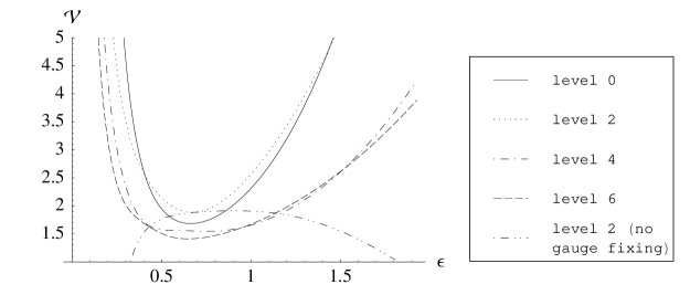
Figure 1: Results of level truncation in the Siegel gauge up to level 6 and level truncation without gauge fixing up to level 2.

While it is not clear whether the result of level truncation converges, we can find some evidence for the existence of a D25-brane solution with finite energy density from the figure. First, the result of level 2 in the Siegel gauge is very close to that of level 2 without gauge fixing when $\epsilon\simeq 0.65$. This indicates that the D25-brane solution can be found in the Siegel gauge at least when $\epsilon\simeq 0.65$. Second, the results are reasonably stable in the range $\epsilon\simeq 0.65$ both when we change the parameter $\epsilon$ and when we increase the level. Not only the energy density but also the values of the parameters such as $x$, $u$, and $v$ do not change rapidly when the level is increased. Several values of ${\cal V}$ are tabulated in table 1.

Table 1: Level truncation up to level 6.

$\epsilon$	Level 0	level 2 (no gauge fixing)	level 2	level 4	level 6
$0.2$	$12.5016$	$-3.11724$	$6.39057$	$4.22023$	$3.15620$
$0.4$	$2.62057$	$1.52154$	$2.58262$	$1.72038$	$1.69360$
$0.6$	$1.71580$	$1.85186$	$1.92678$	$1.56150$	$1.42052$
$0.8$	$1.80139$	$1.90758$	$2.00495$	$1.54859$	$1.47134$
$1$	$2.31058$	$1.90766$	$2.56418$	$1.65508$	$1.67246$

Although the actions with different values of $\epsilon$ are all equivalent, level truncation does not necessarily work equally well for all $\epsilon$. A similar phenomenon was observed in [34], where level truncation with different kinetic operators obtained from $Q_{B}$ by field redefinition was studied. Our results indicate that level truncation works well when $\epsilon\simeq 0.65$. Furthermore, the range of $\epsilon$ where ${\cal V}$ is stable seems to become wider as the level is increased. This qualitative behavior is in fact what we expected from the structure of $Q_{f}(\epsilon)$. When $\epsilon$ is of $O(1)$, the coefficients in front of $Q_{2n}+Q_{-2n}$ decay fast as $n$ becomes large. On the other hand, they do not decay fast when $\epsilon$ is small or large. We therefore do not expect level truncation to work well in these regions of $\epsilon$.

As we mentioned before, the energy density diverges as $1/\epsilon^{3}$ for small $\epsilon$ and as $\epsilon^{3}$ for large $\epsilon$ at level 0. The numerical results in the Siegel gauge indicate that this is also the case at higher levels, but the coefficients in front of $\epsilon^{\pm 3}$ decrease as the level is increased. At level 2 the coefficients are suppressed by a factor of roughly $3.7$ compared to level 0. They are further suppressed by a factor of $2.5$ from level 2 to level 4 and by another factor of $2$ from level 4 to level 6. Although we do not expect that level truncation provides a good approximation for small or large $\epsilon$ when the truncation level stays as low as 6 and it is not even clear if the solution exists in the Siegel gauge for all $\epsilon$, this tendency of suppression seems to be in favor of the existence of a solution with finite energy density rather than divergent energy density.

In the case of level-2 truncation without gauge fixing, there are two other branches where the energy density stays positive for any $\epsilon$ and diverges as $1/\epsilon^{3}$ for small $\epsilon$ and as $\epsilon^{3}$ for large $\epsilon$. However, the smallest values of ${\cal V}$ on these branches are approximately 36 and 110, and the values of $x$ for these solutions are not close to that of the level-0 solution. On the other hand, the energy density ${\cal V}$ and the parameters $x$, $u$, and $v$ on the branch chosen in figure 1 are very close to those of the solution in the Siegel gauge at level 2 when $\epsilon\simeq 0.65$. An unappealing property of this branch is that the energy density turns negative for small $\epsilon$ and goes to zero for large $\epsilon$. While we do not expect that level truncation is a good approximation for these regions of $\epsilon$ when the truncation level is very low, it would be important to confirm that these behaviors are artifacts of truncation.

To summarize, the analysis of level truncation seems to indicate the existence of a solution with finite energy density $\cal V$ of $O(1)$. This approximation scheme seems to work well for $\epsilon\simeq 0.65$, while it does not work well for small or large $\epsilon$, at least when the truncation level is low. We expect that the solution will improve as the truncation level is increased, and the parameter region of $\epsilon$ where level truncation works well may become wider at higher orders. It will not be promising, however, to study the limit $\epsilon\to 0$ by level truncation since higher modes of the kinetic operator are not suppressed. We will study this region using a different method in the next subsection.

3.2 Solution using the butterfly state

We have seen that level truncation does not seem to work for small $\epsilon$. On the other hand, it turns out that the method developed in [19] to solve Witten’s string field theory can be used to solve the equation of motion when $\epsilon$ is small, providing an independent test for the existence of a solution with finite energy density. It is also interesting to study the case with small $\epsilon$ because this is the limit where the kinetic operator becomes the singular midpoint $c$-ghost insertion and we can study the contributions from subleading terms.

The ansatz for the solution takes the form of the regulated butterfly state with an operator insertion at the midpoint of the boundary. Let us define $\left|B_{t}({\cal O})\right\rangle$ by

$$\left\langle\phi|B_{t}({\cal O})\right\rangle=\left\langle I\circ f_{t}\circ\phi(0)\,{\cal O}(0)\right\rangle$$ (3.12)

for any state $\left|\phi\right\rangle$ in the Fock space, where

$$f_{t}(\xi)=\frac{\xi}{\sqrt{1+t^{2}\xi^{2}}}\,,\qquad I(\xi)=-\frac{1}{\xi}\,.$$ (3.13)

As in the case of the regulated butterfly state $\left|B_{t}\right\rangle$, the state $\left|B_{t}({\cal O})\right\rangle$ itself becomes singular in the limit $t\to 1$, but its inner product with a state $\left|\phi\right\rangle$ in the Fock space has a finite limit, which we denote by $\left\langle\phi|B({\cal O})\right\rangle$:

$$\left\langle\phi|B({\cal O})\right\rangle=\lim_{t\to 1}\left\langle\phi|B_{t}({\cal O})\right\rangle=\left\langle I\circ f_{B}\circ\phi(0)\,{\cal O}(0)\right\rangle,$$ (3.14)

where

$$f_{B}(\xi)=\frac{\xi}{\sqrt{1+\xi^{2}}}\,.$$ (3.15)

We will show that $\left|B_{t}(c)\right\rangle$ with an appropriate normalization solves the equation of motion up to $O(\sqrt{\epsilon})$ if we take $t\to 1$ as $\epsilon\to 0$ with $\epsilon/(1-t)$ kept finite.

The quantity $\left\langle\phi|B_{t}(c)\ast B_{t}(c)\right\rangle$ has been computed in [19] and is given by

$$\left\langle\phi|B_{t}(c)\ast B_{t}(c)\right\rangle=\frac{4\sqrt{2}}{3^{1/4}}\sqrt{1-t}\left\langle\phi|B(c\partial c)\right\rangle+O\left((1-t)^{3/2}\right).$$ (3.16)

Let us compute $\left\langle\phi|Q_{f}(\epsilon)|B_{t}(c)\right\rangle$. The function $f(\xi)$ can be written in the coordinate $z=I\circ f_{t}(\xi)$ as

$$f(z)=f(\xi(z))=-\frac{\epsilon^{2}[z^{2}-(1+t^{2})]^{2}}{[(1+\epsilon)(z^{2}-t^{2})+(1-\epsilon)][(1-\epsilon)(z^{2}-t^{2})+(1+\epsilon)]}\,.$$ (3.17)

The double zeros are at $z=\pm\sqrt{1+t^{2}}$, the poles are at

$$z^{2}=t^{2}-\frac{1-\epsilon}{1+\epsilon}\,,\qquad z=\pm i\sqrt{\frac{1+\epsilon}{1-\epsilon}-t^{2}}\,,$$ (3.18)

and the open-string midpoint is at $z=\pm i\sqrt{1-t^{2}}$. The action of the kinetic operator $Q_{f}(\epsilon)$ on an operator at the origin ${\cal O}(0)$ is given by

$$Q_{f}(\epsilon)\cdot{\cal O}(0)\equiv\oint\frac{dz}{2\pi i}\biggl{[}\,f(z)\,j_{B}(z)\,{\cal O}(0)-\frac{f^{\prime}(z)^{2}}{f(z)}\,c(z)\,{\cal O}(0)\,\biggr{]}\,,$$ (3.19)

where the contour encircles the origin and the poles at $z^{2}=t^{2}-(1-\epsilon)/(1+\epsilon)$ counterclockwise. The other poles are located outside the contour. Let us define

$$p^{2}=t^{2}-\frac{1-\epsilon}{1+\epsilon}\,.$$ (3.20)

Then $f(z)$ can be written in the same form as (2.14) using $p$:

$$f(z)=-\frac{\epsilon^{2}}{1-\epsilon^{2}}\frac{\left(z^{2}-p^{2}-\displaystyle{\frac{2}{1+\epsilon}}\right)^{2}}{(z^{2}-p^{2})\left(z^{2}-p^{2}+\displaystyle{\frac{4\,\epsilon}{1-\epsilon^{2}}}\right)}\,.$$ (3.21)

Note that $f(z)$ depends on $t$ only through $p$. The poles inside the contour are located at $\pm p$. The value of $p^{2}$ can be both positive and negative depending on $t$ and $\epsilon$. In particular, when $p^{2}=0$, the two single poles become a double pole at the origin. We have to study this case separately.

Let us first consider the case where $p^{2}\neq 0$. Since $f(\xi)$ in (2.14) and $f(z)$ in (3.21) take the same form, $f(z)$ and $-f^{\prime}(z)^{2}/f(z)$ can be expanded about $z=\pm p$ as in (2.16) and (2.17), respectively, with $\xi$ replaced by $z$. Consequently, $Q_{f}(\epsilon)$ in the $z$ coordinate can be written in the same form as (2.18) with $\xi$ replaced by $z$. It is given by local insertions of $j_{B}(\pm p)$, $c(\pm p)$, $\partial c(\pm p)$ and $\partial^{2}c(\pm p)$ with $p$ defined by (3.20) and integrals around the origin. When $\epsilon$ is small and $t$ is close to 1, $p^{2}$ is small. In this case, the action of $Q_{f}(\epsilon)$ on an operator at the origin can be evaluated using OPE’s. It is convenient to introduce a parameter $\eta$ defined by

$$\eta=\frac{1+t^{2}}{1-t^{2}}\,\epsilon\,,$$ (3.22)

and we will consider the case where $\eta$ is of $O(1)$. Namely, $\epsilon$ and $1-t$ are of the same order and related by

$$\epsilon=\eta\,(1-t)+O((1-t)^{2})\,,\qquad 1-t=\frac{\epsilon}{\eta}+O(\epsilon^{2})\,.$$ (3.23)

In this case, $p^{2}$ is given by

$$p^{2}=\frac{2\,\epsilon\,(\eta-1)}{(\eta+\epsilon)(1+\epsilon)}=2\left(1-\frac{1}{\eta}\right)\epsilon+O(\epsilon^{2})\,.$$ (3.24)

Therefore, $p$ is of $O(\sqrt{\epsilon})$. In the computation of $\langle\phi|Q_{f}(\epsilon)|B_{t}(c)\rangle$, the operator inserted at the origin is $c$, and the relevant OPE’s are

$$j_{B}(z)\,c(0) = \frac{1}{z}\,c\partial c(0)+O(z^{0})\,,$$ (3.25)

$$c(z)\,c(0) = -z\,c\partial c(0)+O(z^{2})\,,$$ (3.26)

$$\partial c(z)\,c(0) = -c\partial c(0)+O(z)\,,$$ (3.27)

$$\partial^{2}c(z)\,c(0) = -c\partial^{2}c(0)+O(z)\,.$$ (3.28)

We compute the leading term of $\langle\phi|Q_{f}(\epsilon)|B_{t}(c)\rangle$ for small $\epsilon$, which is of $O(\epsilon^{0})$. The relevant part of $Q_{f}(\epsilon)\cdot c(0)$ to this order is

$$Q_{f}(\epsilon)\cdot c(0) = -\frac{\epsilon}{2\,p}(j_{B}(p)-j_{B}(-p))\,c(0)+\oint_{C_{0}}\frac{dz}{2\pi i}\,f(z)\,j_{B}(z)\,c(0)+\frac{p^{2}+\epsilon}{4\,p^{2}}(\partial c(p)+\partial c(-p))\,c(0)$$ (3.29)

$$-\frac{p^{4}-\epsilon\,p^{2}+\epsilon^{2}}{4\,\epsilon\,p^{3}}(c(p)-c(-p))\,c(0)-\oint_{C_{0}}\frac{dz}{2\pi i}\,\frac{f^{\prime}(z)^{2}}{f(z)}\,c(z)\,c(0)+O(\epsilon)\,,$$

where the contour $C_{0}$ encircles the origin counterclockwise. The functions $f(z)$ and $-f^{\prime}(z)^{2}/f(z)$ are expanded about the origin when $p^{2}\neq 0$ as follows:

$$f(z) = -\frac{\epsilon^{2}\,(2+p^{2}+\epsilon\,p^{2})^{2}}{p^{2}\,(1+\epsilon)^{2}\,(p^{2}-4\,\epsilon-\epsilon^{2}\,p^{2})}+O(z^{2})=\left[\,-\frac{4\,\epsilon^{2}}{p^{2}\,(p^{2}-4\,\epsilon)}+O(\epsilon)\,\right]+O(z^{2})\,,$$ (3.30)

$$-\frac{f^{\prime}(z)^{2}}{f(z)} = O(z^{2})\,.$$ (3.31)

Therefore, $Q_{f}(\epsilon)\cdot c(0)$ is given by

$$Q_{f}(\epsilon)\cdot c(0) = \left[\,-\frac{\epsilon}{p^{2}}-\frac{4\,\epsilon^{2}}{p^{2}\,(p^{2}-4\,\epsilon)}-\frac{p^{2}+\epsilon}{2\,p^{2}}+\frac{p^{4}-\epsilon\,p^{2}+\epsilon^{2}}{2\,\epsilon\,p^{2}}\,\right]\,c\partial c(0)+O(\epsilon)$$ (3.32)

$$= \left[\,\frac{\eta}{2\,(1+\eta)}-\frac{1}{\eta}\,\right]c\partial c(0)+O(\epsilon)\,,$$

and $\langle\phi|Q_{f}(\epsilon)|B_{t}(c)\rangle$ is

$$\langle\phi|Q_{f}(\epsilon)|B_{t}(c)\rangle=\left[\,\frac{\eta}{2\,(1+\eta)}-\frac{1}{\eta}\,\right]\langle\phi|B_{t}(c\partial c)\rangle+O(\epsilon)=\left[\,\frac{\eta}{2\,(1+\eta)}-\frac{1}{\eta}\,\right]\langle\phi|B(c\partial c)\rangle+O(\epsilon)\,.$$ (3.33)

While the operator $Q_{f}(\epsilon)$ in $\langle\phi_{1}|Q_{f}(\epsilon)|\phi_{2}\rangle$ with $|\phi_{1}\rangle$ and $|\phi_{2}\rangle$ in the Fock space is dominated by the midpoint $c$-ghost insertion when $\epsilon$ is small, this is not the case for $\langle\phi|Q_{f}(\epsilon)|B_{t}(c)\rangle$. Contributions from subleading terms in $Q_{f}(\epsilon)$ are nonvanishing in this computation.

Let us next consider the case where $p^{2}=0$, which corresponds to $\eta=1$. In this case, $t$ and $\epsilon$ are related by

$$t=\sqrt{\frac{1-\epsilon}{1+\epsilon}}\,,$$ (3.34)

and the two single poles inside the contour become a double pole at the origin. The computation in fact simplifies in this case. The functions $f(z)$ and $-f^{\prime}(z)^{2}/f(z)$ are expanded about the origin as follows:

$$f(z) = -\frac{\epsilon}{(1+\epsilon)^{2}}\frac{1}{z^{2}}+\frac{1+3\,\epsilon}{4\,(1+\epsilon)}-\frac{(1+\epsilon)^{2}}{16\,\epsilon}\,z^{2}+O(z^{4})\,,$$ (3.35)

$$-\frac{f^{\prime}(z)^{2}}{f(z)} = \frac{4\,\epsilon}{(1+\epsilon)^{2}}\frac{1}{z^{4}}+\frac{1+3\,\epsilon}{1+\epsilon}\frac{1}{z^{2}}+\left(-\frac{1}{2\,\epsilon}+\frac{3\,\epsilon}{2}\right)+O(z^{2})\,.$$ (3.36)

Therefore, $Q_{f}(\epsilon)\cdot c(0)$ is

$$Q_{f}(\epsilon)\cdot c(0)=-\frac{3\,(1+3\,\epsilon)}{4\,(1+\epsilon)}\,c\partial c(0)+O(\epsilon)=-\frac{3}{4}\,c\partial c(0)+O(\epsilon)\,,$$ (3.37)

and $\left\langle\phi|Q_{f}(\epsilon)|B_{t}(c)\right\rangle$ is

$$\left\langle\phi|Q_{f}(\epsilon)|B_{t}(c)\right\rangle=-\frac{3}{4}\left\langle\phi|B_{t}(c\partial c)\right\rangle+O(\epsilon)=-\frac{3}{4}\left\langle\phi|B(c\partial c)\right\rangle+O(\epsilon)\,.$$ (3.38)

This coincides with (3.33) when $\eta=1$. Therefore, (3.33) is valid for any $\eta$ including $\eta=1$.

The leading term of $\langle\phi|Q_{f}(\epsilon)|B_{t}(c)\rangle$ is proportional to that of $\left\langle\phi|B_{t}(c)\ast B_{t}(c)\right\rangle$ in (3.16). If we define

$$|\Psi^{(0)}\rangle=x\left|B_{t}(c)\right\rangle$$ (3.39)

with

$$x=-\frac{3^{1/4}\sqrt{\eta}}{4\sqrt{2}}\left[\frac{\eta}{2\,(1+\eta)}-\frac{1}{\eta}\right]\frac{1}{\sqrt{\epsilon}}\qquad\hbox{and}\qquad t=\sqrt{\frac{\eta-\epsilon}{\eta+\epsilon}}\,,$$ (3.40)

the state $|\Psi^{(0)}\rangle$ solves the equation of motion up to $O(\sqrt{\epsilon})$:

$$\langle\phi|Q_{f}(\epsilon)|\Psi^{(0)}\rangle+\langle\phi|\Psi^{(0)}\ast\Psi^{(0)}\rangle=O(\sqrt{\epsilon})$$ (3.41)

for any state $\left|\phi\right\rangle$ in the Fock space. If we take the limit $\epsilon\to 0$, the state $|\Psi^{(0)}\rangle$ formally solves the equation of motion exactly. However, the state $\left|B_{t}(c)\right\rangle$ becomes singular and the coefficient diverges as $1/\sqrt{\epsilon}$ in the limit so that we do not intend to take the strict $\epsilon\to 0$ limit. On the other hand, the state $|\Psi^{(0)}\rangle$ is well defined as long as $\epsilon$ is finite. If we choose $\epsilon$ to be 0.0001, for example, the equation of motion is solved with fairly good precision for any state $\left|\phi\right\rangle$ in the Fock space.

Since the solution is outside the Fock space, it is a nontrivial question if the equation of motion can be satisfied when it is contracted with the solution itself. We can study this by evaluating the following dimensionless quantity:

$${\cal R}[\Psi]\equiv-\frac{\langle\Psi|Q_{f}(\epsilon)|\Psi\rangle}{\langle\Psi|\Psi\ast\Psi\rangle}\,.$$ (3.42)

If ${\cal R}$ for the solution is close to $1$, the equation of motion contracted the solution itself is satisfied with good accuracy. It is also a nontrivial question if the normalized energy density ${\cal V}$ is well defined and finite. Let us compute ${\cal R}$ and ${\cal V}$ for the solution $|\Psi^{(0)}\rangle$:

$${\cal R}[\Psi^{(0)}] = -\frac{\langle B_{t}(c)|Q_{f}(\epsilon)|B_{t}(c)\rangle}{x\,\langle B_{t}(c)|B_{t}(c)\ast B_{t}(c)\rangle}\,,$$ (3.43)

$${\cal V}[\Psi^{(0)}] = 2\pi^{2}\left[\frac{x^{2}}{2}\langle B_{t}(c)|Q_{f}(\epsilon)|B_{t}(c)\rangle_{density}+\frac{x^{3}}{3}\langle B_{t}(c)|B_{t}(c)\ast B_{t}(c)\rangle_{density}\right]\,,$$ (3.44)

with $x$ and $t$ given in (3.40). The quantity $\left\langle B_{t}(c)|B_{t}(c)\ast B_{t}(c)\right\rangle$ has been computed in [19] and is given by

$$\left\langle B_{t}(c)|B_{t}(c)\ast B_{t}(c)\right\rangle_{density}=-\left(\frac{3\sqrt{3}}{4}\right)^{3}(1-t^{4})^{3/2}.$$ (3.45)

We need to compute the inner product $\left\langle B_{t}(c)|Q_{f}(\epsilon)|B_{t}(c)\right\rangle$. The computation is closely related to that of $\left\langle B_{t}(c)|Q_{B}|B_{t}(c)\right\rangle$ in [19].

When we deal with the star multiplication of the regulated butterfly state, it is convenient to use the $\hat{z}$ coordinate [11] defined by

$$\hat{z}=\arctan\xi\,.$$ (3.46)

In the $\hat{z}$ coordinate, the left and right halves of the open string of the regulated butterfly state are mapped to semi-infinite lines parallel to the imaginary axis in the upper-half plane. Thus gluing can be performed simply by translation. We glue two regulated butterfly states together in this way. We then map the resulting surface to an upper-half plane by a conformal transformation, and the coordinate of the upper-half plane was called $z$ in [12]. The relation between the $z$ coordinate and the $\xi$ coordinate can be read off from (C.15) and (C.16) in [12] and is given by

$$\left(\frac{2\,\xi}{1-\xi^{2}}\right)^{2}=\frac{(1-z^{2})^{2}-4\,q^{2}\,z^{2}}{4\,(1+q^{2})\,z^{2}}\,,$$ (3.47)

where

$$q=\frac{2\,t}{1-t^{2}}\,.$$ (3.48)

Since $f(\xi)$ can be written as

$$f(\xi)=\left[1-\frac{1}{\epsilon^{2}}\left\{1+\left(\frac{2\,\xi}{1-\xi^{2}}\right)^{2}\right\}\right]^{-1},$$ (3.49)

the form of $Q_{f}(\epsilon)$ in the $z$ coordinate can be easily derived using (3.47). The expression of the inner product $\left\langle B_{t}(c)|Q_{f}(\epsilon)|B_{t}(c)\right\rangle$ further simplifies in the $w$ coordinate defined by

$$w=\frac{z-1}{z+1}\,.$$ (3.50)

The function $f(\xi)$ can be written in the $w$ coordinate as follows:

$$f(w) = f(\xi(w))=\left[1-\frac{(1-t^{2})^{2}}{\epsilon^{2}\,(1+t^{2})^{2}}\left\{1+\left(\frac{2\,w}{1-w^{2}}\right)^{2}\right\}\right]^{-1}$$ (3.51)

$$= \left[1-\frac{1}{\eta^{2}}\left\{1+\left(\frac{2\,w}{1-w^{2}}\right)^{2}\right\}\right]^{-1},$$

where we have used the parameter $\eta$ introduced in (3.22). The conformal factor of the $c$ ghost associated with the mapping to the $z$ coordinate has been computed in [12, 19]. The two $c$ ghosts are mapped to

$$\frac{\sqrt{1-t^{4}}}{2}\,c(\pm 1)$$ (3.52)

in the $z$ coordinate. They are further mapped to $\sqrt{1-t^{4}}\,c(0)$ and $\sqrt{1-t^{4}}\,I\circ c(0)$ in the $w$ coordinate. Therefore, the computation of $\left\langle B_{t}(c)|Q_{f}(\epsilon)|B_{t}(c)\right\rangle$ reduces to that of $\left\langle 0|c_{-1}Q_{f}(\eta)c_{1}|0\right\rangle$. The latter has already been calculated in the previous subsection so that $\left\langle B_{t}(c)|Q_{f}(\epsilon)|B_{t}(c)\right\rangle$ is given by

$$\left\langle B_{t}(c)|Q_{f}(\epsilon)|B_{t}(c)\right\rangle_{density} = (1-t^{4})\langle 0|c_{-1}Q_{f}(\eta)c_{1}|0\rangle_{density}$$ (3.53)

$$= (1-t^{4})\left(-\frac{\eta}{1+\eta}+\frac{1+3\,\eta^{2}}{2\,\eta}\right).$$

We are now ready to evaluate ${\cal R}[\Psi^{(0)}]$ and ${\cal V}[\Psi^{(0)}]$. Combining (3.40), (3.45), and (3.53), they are given by

$${\cal R}[\Psi^{(0)}] = 2^{15/2}\cdot 3^{-19/4}\left(\frac{1+3\eta^{2}}{2\eta}-\frac{\eta}{1+\eta}\right)\left(\frac{1}{\eta}-\frac{\eta}{2(1+\eta)}\right)^{-1}+O(\epsilon)\,,$$ (3.54)

$${\cal V}[\Psi^{(0)}] = 2\pi^{2}\left(\frac{1}{\eta}-\frac{\eta}{2(1+\eta)}\right)^{2}\left[\frac{\sqrt{3}}{16}\left(\frac{1+3\eta^{2}}{2\eta}-\frac{\eta}{1+\eta}\right)-2^{-21/2}\cdot 3^{17/4}\left(\frac{1}{\eta}-\frac{\eta}{2(1+\eta)}\right)\right]+O(\epsilon)\,.$$

For finite $\eta$ the ratio ${\cal R}[\Psi^{(0)}]$ is of $O(1)$ and has the value ${\cal R}[\Psi^{(0)}]=1$ when $\eta\simeq 0.657104$. This means that while the equation of motion contracted with a state in the Fock space can be solved up to $O(\sqrt{\epsilon})$ for any $\eta$, the equation of motion contracted with the solution itself can be satisfied only when $\eta\simeq 0.657104$. We therefore think that our ansatz works well only when $\eta\simeq 0.657104$. The energy density ${\cal V}$ is well defined and finite even in the limit $\epsilon\to 0$. Its value in the limit $\epsilon\to 0$ when $\eta\simeq 0.657104$ is ${\cal V}\simeq 1.68454$. This is close to the results obtained by level truncation for finite $\epsilon$, while we are now looking at $Q_{f}(\epsilon)$ with small $\epsilon$. This is exactly what we expected since the actions with different values of $\epsilon$ are equivalent and the energy density should be independent of $\epsilon$. It is also interesting to note that ${\cal V}[\Psi^{(0)}]$ in the limit $\epsilon\to 0$ as a function of $\eta$ has a stationary point at $\eta\simeq 0.653151$ where ${\cal V}[\Psi^{(0)}]\simeq 1.6847$. This is very close to the point where ${\cal R}[\Psi^{(0)}]=1$. The energy density is therefore rather stable in the region of $\eta$ where our ansatz is valid.

We have also computed the solution at the next-to-leading order. The computations are summarized in appendix B. As in the case of solving Witten’s string field theory using this method [19], we found many solutions for a given $\eta$. While the dimensionless ratio ${\cal R}$ is generically not close to $1$, we found one branch of solutions where ${\cal R}\simeq 1$. The result is summarized in table 2. Remarkably, ${\cal R}$ becomes close to $1$ around $\eta\simeq 0.65$ as in the case of the leading-order solution. The energy density at $\eta\simeq 0.65$ is ${\cal V}\simeq 3.14$ and seems a little too large compared with the leading-order result or with the results from level truncation. However, it is in fact quite nontrivial to have obtained the result of $O(1)$ in this numerical analysis since solutions on other branches are generically far away from $O(1)$.

Table 2: ${\cal R}$ and ${\cal V}$ for the solution at the next-to-leading order.

$\eta$	${\cal R}$	${\cal V}$
$0.55$	$0.889736$	$2.89180$
$0.60$	$0.938201$	$3.02575$
$0.65$	$1.00333$	$3.14301$
$0.70$	$1.09325$	$3.21288$
$0.75$	$1.22089$	$3.20464$
$0.80$	$1.41254$	$3.08059$
$0.85$	$1.73586$	$2.77125$
$0.90$	$2.44342$	$2.10526$

As was discussed in [12], the finiteness of the energy density of a solution depends on the subleading structure of the kinetic operator (2.3). We have explicitly demonstrated that our kinetic operator does admit a perturbative solution with finite energy density. Level truncation and the perturbative method using the butterfly state are valid in different parameter regions of $\epsilon$, but both gave qualitatively compatible results with ${\cal V}$ of $O(1)$. We regard this as evidence for the existence of a D25-brane solution with finite energy density.

It was also argued in [12] that contributions to $\left\langle\Psi|Q_{f}(\epsilon)|\Psi\right\rangle$ from subleading terms of the kinetic operator can be of the same order as that from the leading term. It is indeed the case for our kinetic operator. Let us replace $Q_{f}(\epsilon)$ in $\left\langle B_{t}(c)|Q_{f}(\epsilon)|B_{t}(c)\right\rangle$ by its leading term in (2.19). Since $\left\langle B_{t}(c)|Q|B_{t}(c)\right\rangle_{density}=(1-t^{2})^{2}$ as computed in [19], the contribution to $\left\langle B_{t}(c)|Q_{f}(\epsilon)|B_{t}(c)\right\rangle$ from the leading term of $Q_{f}(\epsilon)$ is given by

$$\frac{1}{2\,\epsilon}\left\langle B_{t}(c)|Q|B_{t}(c)\right\rangle_{density}=\frac{1-t^{4}}{2\,\eta}\,.$$ (3.56)

This is different from (3.53). Because subleading terms of $Q_{f}(\epsilon)$ contribute to $\left\langle\phi|Q_{f}(\epsilon)|\Psi\right\rangle$ and $\left\langle\Psi|Q_{f}(\epsilon)|\Psi\right\rangle$, the ratio (1.3) depends on $\eta$ and can be close to 1. We have seen that the ratio (1.3) is in fact close to 1 when $\eta\simeq 0.65$, and thus the problem of the incompatibility between (1.1) and (1.2) has been resolved by subleading terms of $Q_{f}(\epsilon)$.

Level truncation works well when $\epsilon\simeq 0.65$ and the solution based on the butterfly state works well when $\eta\simeq 0.65$. It it interesting to note that these two numbers are so close. This might be explained by the following picture. Let us denote the exact solution in the Siegel gauge at $\epsilon_{\ast}=0.65$ by $\left|\Psi_{\ast}\right\rangle$. Our results of level truncation seem to indicate that $\left|\Psi_{\ast}\right\rangle$ is relatively close to a state in the Fock space. Since the kinetic operators with different values of $\epsilon$ are related by the similarity transformation (2.24), exact solutions for different values of $\epsilon$ are given by $e^{\,bK_{2}}\left|\Psi_{\ast}\right\rangle$, where

$$b=\frac{1}{4}\ln\frac{\epsilon_{\ast}}{\epsilon}\,.$$ (3.57)

The action of the operator $e^{\,bK_{2}}$ on $\left|\Psi_{\ast}\right\rangle$ would be nontrivial, especially for small $b$. However, the state $e^{\,bK_{2}}\left|\Psi_{\ast}\right\rangle$ with large $b$ might be approximated in the following way. It was shown in [10] that the action of $e^{\,bK_{2}}$ on the $SL(2,R)$-invariant vacuum $\left|0\right\rangle$ gives the regulated butterfly state $\left|B_{t}\right\rangle$. The relation between the parameters $b$ and $t$ can be read off from

$$e^{\,bK_{2}}\left|0\right\rangle=\exp\left[-\frac{\tanh(2b)}{2}L_{-2}\right]\left|0\right\rangle$$ (3.58)

and

$$\left|B_{t}\right\rangle=\exp\left(-\frac{t^{2}}{2}L_{-2}\right)\left|0\right\rangle\,.$$ (3.59)

The operator $e^{\,bK_{2}}$ with large $b$ therefore transforms the vacuum $\left|0\right\rangle$ into a regulated butterfly state $\left|B_{t}\right\rangle$ with $t$ close to 1. Since $\left|\Psi_{\ast}\right\rangle$ is expected to be close to a state in the Fock space, the state $e^{\,bK_{2}}\left|\Psi_{\ast}\right\rangle$ with large $b$ might be approximated by a regulated butterfly state $e^{\,bK_{2}}\left|0\right\rangle$ with operator insertions. From (3.58) and (3.59) we can estimate the parameter $t$ of the butterfly state to be

$$t^{2}=\tanh\left(\frac{1}{2}\ln\frac{\epsilon_{\ast}}{\epsilon}\right)=\frac{\epsilon_{\ast}-\epsilon}{\epsilon_{\ast}+\epsilon}\,.$$ (3.60)

Then, $\eta$ defined in (3.22) precisely coincides with $\epsilon_{\ast}$:

$$\eta=\frac{1+t^{2}}{1-t^{2}}\,\epsilon=\epsilon_{\ast}\,.$$ (3.61)

This argument is too simplified, but it could be a qualitative explanation of the coincidence of the two numbers. This picture also naturally explains why we should consider the case with $\eta$ of $O(1)$.

The parameter $\epsilon$ of $Q_{f}(\epsilon)$ and the parameter $t$ of $\left|B_{t}\right\rangle$ are both changed by a transformation generated by $K_{2}$. The butterfly state is special for $Q_{f}(\epsilon)$ among other star-algebra projectors in this respect. The method of [19] based on the butterfly state has been generalized in [35] to use other projectors, and such generalization would be useful for other choices of the function $f$ in $Q_{f}$.

4 Construction of other D-brane solutions

We have obtained evidence that the string field theory with $Q_{f}(\epsilon)$ has a D25-brane solution with finite energy density. Let us now consider other D-brane solutions. In [7], other D-brane solutions were constructed by changing the boundary condition of the surface state. Since the equation of motion no longer factorizes into the matter and ghost sectors in our case, it may seem that the construction of other D-brane solutions becomes nontrivial. We show that changing the boundary condition of the surface state works in our case as well because of a special property of the function $f(\xi)$.

Let us consider our solution based on the regulated butterfly state. Following [7], we insert the following pair of boundary condition changing operators in the $\hat{z}$ coordinate:

$$\sigma^{+}\left(\frac{\pi}{4}+\lambda\right)\,,\qquad\sigma^{-}\left(-\frac{\pi}{4}-\lambda\right)\,,$$ (4.1)

where $\lambda$ is a regularization parameter to be sent to 0. We also need to multiply the state by a factor $(2\lambda)^{2h}$ to solve the equation of motion, where $h$ is the conformal dimension of $\sigma^{\pm}$. After mapping the operator to the coordinate $I\circ f_{t}(\xi)$ and an appropriate rescaling of $\lambda$, our ansatz for the solution can be written as

$$\left\langle\phi|B_{t}^{\sigma}({\cal O})\right\rangle=(2\lambda)^{2h}\left\langle I\circ f_{t}\circ\phi(0)\,\sigma^{+}\left(-\sqrt{1+t^{2}}+\lambda\right)\,{\cal O}(0)\,\sigma^{-}\left(\sqrt{1+t^{2}}-\lambda\right)\right\rangle$$ (4.2)

for any state $\left|\phi\right\rangle$ in the Fock space. Let us consider $\langle\phi|Q_{f}(\epsilon)|B_{t}^{\sigma}({\cal O})\rangle$ and $\langle\phi|B_{t}^{\sigma}({\cal O})\ast B_{t}^{\sigma}({\cal O})\rangle$. A pair of $\sigma^{+}$ and $\sigma^{-}$ approach to each other in $\langle\phi|B_{t}^{\sigma}({\cal O})\ast B_{t}^{\sigma}({\cal O})\rangle$, and the leading term in their OPE cancels one of the two factors of $(2\lambda)^{2h}$. The remaining part of the computation is exactly the same except that the boundary condition has been changed. In the computation of $\langle\phi|Q_{f}(\epsilon)|B_{t}^{\sigma}({\cal O})\rangle$, the action of $Q_{f}(\epsilon)$ on $\sigma^{\pm}$ can potentially produce nonvanishing contributions. Since both $f(z)$ and $f^{\prime}(z)^{2}/f(z)$ are regular at the insertion points of $\sigma^{\pm}$ and the OPE between $c$ and $\sigma^{\pm}$ is trivial, $Q_{f}(\epsilon)\cdot\sigma^{\pm}$ is given by

$$Q_{f}(\epsilon)\cdot\sigma^{\pm}(w) = \oint_{C_{w}}\frac{dz}{2\pi i}\,f(z)\,j_{B}(z)\,\sigma^{\pm}(w)$$ (4.3)

$$= \oint_{C_{w}}\frac{dz}{2\pi i}\,f(z)\left\{\frac{h}{(z-w)^{2}}\,c\sigma^{\pm}(w)+\frac{1}{z-w}\left[h(\partial c)\sigma^{\pm}(w)+c\partial\sigma^{\pm}(w)\right]\right\}$$

$$= h\,f^{\prime}(w)\,c\sigma^{\pm}(w)+f(w)\left[h(\partial c)\sigma^{\pm}(w)+c\partial\sigma^{\pm}(w)\right]\,,$$

where the contour $C_{w}$ encircles $w$ counterclockwise. Since $f(z)$ has a double pole at both ends of the open string, $Q_{f}(\epsilon)\cdot\sigma^{\pm}$ vanishes in the limit $\lambda\to 0$. More explicitly, from the expression of $f(z)$ in the coordinate $z=I\circ f_{t}(\xi)$ we find

$$f(z)\Bigr{|}_{z=\mp\sqrt{1+t^{2}}\pm\lambda}=-(1+t^{2})\epsilon^{2}\lambda^{2}+O(\lambda^{3})\,,$$

$$f^{\prime}(z)\Bigr{|}_{z=\mp\sqrt{1+t^{2}}\pm\lambda}=\mp 2(1+t^{2})\epsilon^{2}\lambda+O(\lambda^{2})\,.$$ (4.4)

Therefore, if $|B_{t}({\cal O})\rangle$ solves the equation

$$\langle\phi|Q_{f}(\epsilon)|B_{t}({\cal O})\rangle+\langle\phi|B_{t}({\cal O})\ast B_{t}({\cal O})\rangle=0$$ (4.5)

for any $\left|\phi\right\rangle$ in the Fock space, $|B_{t}^{\sigma}({\cal O})\rangle$ solves the same equation in the limit $\lambda\to 0$:

$$\langle\phi|Q_{f}(\epsilon)|B_{t}^{\sigma}({\cal O})\rangle+\langle\phi|B_{t}^{\sigma}({\cal O})\ast B_{t}^{\sigma}({\cal O})\rangle=0\,.$$ (4.6)

As in the case of [7], we interpret solutions generated in this way as D-branes with the boundary condition associated with $\sigma^{\pm}$.

This mechanism of generating new solutions in fact works for any solution which consists of a surface state with insertions of $b$, $c$, and the matter part of the energy-momentum tensor which we denote by $T^{m}$. Moreover, it works for any kinetic operator which is made of $T^{m}$, $b$, and $c$ and whose action on the boundary condition changing operators vanishes. In particular, it works for the level-truncation solution for $Q_{f}(\epsilon)$ with $\epsilon$ of $O(1)$. On the other hand, this mechanism does not work for the BRST operator $Q_{B}$. It corresponds to the case where $f(\xi)$ is constant and the action of $Q_{B}$ on the boundary condition changing operators does not vanish. We are also not able to make use of this method to generate other solutions from the formal solution for $Q_{f}(\epsilon)$ with $\epsilon=1$ by Takahashi and Tanimoto [21] because their solution is based on the identity state which does not have any boundary.

Let us next consider energies of solutions constructed in this method. The computation of $\langle B_{t}^{\sigma}({\cal O})|Q_{f}(\epsilon)|B_{t}^{\sigma}({\cal O})\rangle$ can be reduced to that of $\langle B_{t}({\cal O})|Q_{f}(\epsilon)|B_{t}({\cal O})\rangle$ if the contour of the integral in $Q_{f}(\epsilon)$ can be deformed across the boundary condition changing operators. Although $Q_{f}(\epsilon)\cdot\sigma^{\pm}$ vanishes in the limit $\lambda\to 0$, there is a potential subtlety coming from the existence of $\sigma^{\mp}$ from the other state. In a coordinate where the open-string endpoint is located at the origin, the quantity in question is given by

$$\hskip-56.9055pt(2\lambda)^{2h}\,\sigma^{-}(-\lambda)\,Q_{f}(\epsilon)\cdot\sigma^{+}(\lambda)$$ (4.7)

$$= (2\lambda)^{2h}\,\sigma^{-}(-\lambda)\,\Bigl{\{}h\,f^{\prime}(\lambda)\,c\sigma^{+}(\lambda)+f(\lambda)\left[h(\partial c)\sigma^{+}(\lambda)+c\partial\sigma^{+}(\lambda)\right]\Bigr{\}}\,.$$

The leading term of the OPE $\sigma^{-}(-\lambda)\,\partial\sigma^{+}(\lambda)$ is of $O(\lambda^{-2h-1})$ and is more singular than that of $\sigma^{-}(-\lambda)\,\sigma^{+}(\lambda)$, but the quantity (4.7) still vanishes in the limit $\lambda\to 0$ because $f(\lambda)$ is of $O(\lambda^{2})$. Similarly, we can also show that $(2\lambda)^{2h}\,\left[\,Q_{f}(\epsilon)\cdot\sigma^{-}(-\lambda)\,\right]\,\sigma^{+}(\lambda)$ vanishes in the limit $\lambda\to 0$. Therefore, we can safely deform the contour of the integral in $Q_{f}(\epsilon)$ across any of the boundary condition changing operators. Then, each of the two pairs of adjacent $\sigma^{+}$ and $\sigma^{-}$ can be replaced by $(2\lambda)^{-2h}$, and the two factors of $(2\lambda)^{2h}$ from the normalization of $|B_{t}^{\sigma}({\cal O})\rangle$ are canceled. Similarly, each of the three pairs of adjacent $\sigma^{+}$ and $\sigma^{-}$ in $\langle B_{t}^{\sigma}({\cal O})|B_{t}^{\sigma}({\cal O})\ast B_{t}^{\sigma}({\cal O})\rangle$ can be replaced by $(2\lambda)^{-2h}$, and the three factors of $(2\lambda)^{2h}$ from the normalization of $|B_{t}^{\sigma}({\cal O})\rangle$ are canceled. In both cases, the remaining computation is the same except that the boundary condition has been changed. Since the operators ${\cal O}$ and $Q_{f}(\epsilon)$ consist of $T^{m}$, $b$, and $c$, either of $\langle B_{t}^{\sigma}({\cal O})|Q_{f}(\epsilon)|B_{t}^{\sigma}({\cal O})\rangle$ and $\langle B_{t}^{\sigma}({\cal O})|B_{t}^{\sigma}({\cal O})\ast B_{t}^{\sigma}({\cal O})\rangle$ is a correlation function of operators $T^{m}$, $b$, and $c$. The ghost part of the correlation is obviously independent of the boundary condition. The matter part is made of correlation functions of $T^{m}$, which are completely determined by the conformal symmetry except for the overall normalization given by the disk partition function ${\cal Z}_{\sigma}=\left\langle 1\right\rangle$ with the boundary condition associated with $\sigma^{\pm}$. Therefore, we find

$$\frac{\langle B_{t}^{\sigma}({\cal O})|Q_{f}(\epsilon)|B_{t}^{\sigma}({\cal O})\rangle}{\langle B_{t}^{\sigma^{\prime}}({\cal O})|Q_{f}(\epsilon)|B_{t}^{\sigma^{\prime}}({\cal O})\rangle}=\frac{\langle B_{t}^{\sigma}({\cal O})|B_{t}^{\sigma}({\cal O})\ast B_{t}^{\sigma}({\cal O})\rangle}{\langle B_{t}^{\sigma^{\prime}}({\cal O})|B_{t}^{\sigma^{\prime}}({\cal O})\ast B_{t}^{\sigma^{\prime}}({\cal O})\rangle}=\frac{{\cal Z}_{\sigma}}{{\cal Z}_{\sigma^{\prime}}}$$ (4.8)

for any pair of boundary conditions associated with $\sigma^{\pm}$ and $\sigma^{\prime\pm}$. It follows from (4.8) that ratios of energies of solutions are given by ratios of disk partition functions. Since the disk partition function is proportional to the corresponding D-brane tension [36, 37, 38, 39, 40], ratios of D-brane tensions are correctly reproduced just as in the case of [7]. In our case, however, their assumption of the factorization into the matter and ghost sectors has been relaxed. Again, this argument holds for any solution which consists of a surface state with insertions of $T^{m}$, $b$, and $c$ when the kinetic operator is made of $T^{m}$, $b$, and $c$ and its action on the boundary condition changing operators vanishes. Furthermore, the derivation of (4.8) did not require the equation of motion to be satisfied so that we can use (4.8) even for an approximate solution such as the level-truncation solution or the one based on the regulated butterfly state.

5 Discussion

The conjecture in [1] that the kinetic operator ${\cal Q}$ can be made purely of ghost fields was motivated by universality. Namely, the open string field theory action at the tachyon vacuum should be independent of the matter sector, although a reference matter boundary CFT with $c=26$ is still necessary to formulate string field theory. The kinetic operator $Q_{f}(\epsilon)$ apparently depends on the matter boundary CFT and the resulting string field theory may not seem to be universal. However, when the kinetic operator is given by $Q_{f}(\epsilon)$, the open-string end points do not propagate in the Siegel gauge because of the zeros of $f(\xi)$ at the open-string end points [41, 20, 42]. It is expected that the resulting Riemann surfaces are effectively closed and the amplitudes they express could be independent of the open-string boundary condition in this way.

On the other hand, the open-string midpoint does propagate in the Siegel gauge. This resolves the following problematic singular nature of the midpoint $c$-ghost insertion. Consider the one-loop effective action of vacuum string field theory evaluated at the D25-brane solution. It should reproduce the ordinary amplitudes integrated over the cylinder modulus. However, when the kinetic operator is made purely of ghost fields, not only the end points but also the whole open string does not propagate. Then whatever state we may take for the D25-brane solution, it seems that only degenerated cylinders can be generated because the open-string midpoint does not propagate [43]. The kinetic operator $Q_{f}(\epsilon)$ seems to avoid this problem without breaking universality.

The argument in section 4 only requires that the kinetic operator should consist of $b$, $c$, and $T^{m}$ and that the action of the kinetic operator on boundary condition changing operators at the open-string end points gives vanishing contributions. The kinetic operator $Q_{f}(\epsilon)$ considered in this paper is one particular example, and there will be other operators satisfying these requirements. For example, we can choose a different function $f(\xi)$ for $Q_{f}$. It is an important open question if they are equivalent or not. There may also be operators satisfying the requirements other than the ones constructed by Takahashi and Tanimoto. However, it is very nontrivial to construct consistent kinetic operators having the nilpotency and the derivation property out of $b$, $c$, and $T^{m}$ in other ways. As far as we can see there are no obvious problems with the kinetic operators $Q_{f}(\epsilon)$. These operators could be exact kinetic operators at the tachyon vacuum.

Once the singular pure-ghost theory of Gaiotto, Rastelli, Sen and Zwiebach is related to a regular theory by field redefinition, it is not surprising that the D25-brane solution has finite energy density. A nontrivial question is if the energy density ${\cal E}$ and the on-shell three-tachyon coupling constant $g_{T}$ on a D25-brane are related by the formula ${\cal E}=1/(2\pi^{2}\alpha^{\prime 3}g_{T}^{2})$. This relation, together with the correct open-string mass spectrum, can be derived if we assume the matter-ghost factorization [17]. It is an important open problem if this relation and the mass spectrum can be derived for the theory with the operator $Q_{f}(\epsilon)$.

Appendix A. Conformal field theory formulation of string field theory

In the CFT formulation of string field theory [13, 14], an open string field is represented as a wave functional obtained by a path integral over a certain region in a Riemann surface. For example, a state $\left|\phi\right\rangle$ in the Fock space can be represented as a wave functional on the arc $|\xi|=1$ in the upper-half complex plane of $\xi$ by path-integrating over the interior of the upper half of the unit disk $|\xi|<1$ with the corresponding operator $\phi(0)$ inserted at the origin and with the boundary condition of the open string imposed on the part of the real axis $-1\leq\xi\leq 1$. A more general class of states such as the regulated butterfly state can be defined by a path integral over a different region of a Riemann surface with a boundary and with possible operator insertions. When we parametrize the open string on the arc as $\xi=e^{i\theta}$ with $0\leq\theta\leq\pi$, we refer to the region $\pi/2\leq\theta\leq\pi$ as the left half of the open string, and to the region $0\leq\theta\leq\pi/2$ as the right half of the open string. We also refer to the point $\theta=\pi/2$ as the open-string midpoint.

We use the standard definitions [4] of the inner product $\left\langle\phi_{1}|\phi_{2}\right\rangle$ and the star product $\left|\phi_{1}\ast\phi_{2}\right\rangle$. The state $\left|\phi_{1}\ast\phi_{2}\right\rangle$ is defined by gluing together the right half of the open string of $\left|\phi_{1}\right\rangle$ and the left half of the open string of $\left|\phi_{2}\right\rangle$. Gluing can be performed by conformal transformations which map the two regions to be glued together into the same region. The inner product $\left\langle\phi_{1}|\phi_{2}\right\rangle$ is defined by gluing the left and right halves of the open string of $\left|\phi_{1}\ast\phi_{2}\right\rangle$.

We use the doubling trick throughout the paper. For example, $bc$ ghosts on the upper-half plane are extended to the lower-half plane by $c(\bar{z})=\tilde{c}(z)$ and $b(\bar{z})=\tilde{b}(z)$. The normalization of correlation functions is given by

$$\left\langle c(z_{1})\,c(z_{2})\,c(z_{3})\right\rangle=(z_{1}-z_{2})(z_{1}-z_{3})(z_{2}-z_{3})\int d^{26}x\,.$$ (A.1)

In this paper, we only consider correlation functions which are independent of space-time coordinates so that the space-time volume always factors out. We use the subscript $density$ to denote a quantity divided by the volume factor of space-time. For example, (A.1) is written as

$$\left\langle c(z_{1})\,c(z_{2})\,c(z_{3})\right\rangle_{density}=(z_{1}-z_{2})(z_{1}-z_{3})(z_{2}-z_{3})\,.$$ (A.2)

The normalization of a state $\left|\phi\right\rangle$ in the Fock space is fixed by the condition that the $SL(2,R)$-invariant vacuum $\left|0\right\rangle$ corresponds to the identity operator. From the normalization of correlation functions (A.1) and the standard mode expansion of $c$ on the unit circle given by

$$c_{n}=\oint\frac{dz}{2\pi i}\,z^{n-2}\,c(z)\,,$$ (A.3)

the normalization of the inner product is then fixed as follows:

$$\left\langle 0|c_{-1}c_{0}c_{1}|0\right\rangle_{density}=1\,.$$ (A.4)

Appendix B. Solution at the next-to-leading order using the butterfly state

Our ansatz for the solution at the next-to-leading order is

$$|\Psi^{(2)}\rangle=\frac{x}{\sqrt{1-t}}\left|B_{t}(c)\right\rangle+\sqrt{1-t}\left[u\,|B_{t}(\partial^{2}c)\rangle+v\,\left|B_{t}(cT^{m})\right\rangle+w\,\left|B_{t}({\rm:}\,bc\partial c\,{\rm:})\right\rangle\right],$$ (B.1)

where $T^{m}$ is the matter part of the energy-momentum tensor and $x$, $u$, $v$, and $w$ are parameters to be determined.

The quantity $\langle\phi|Q_{f}(\epsilon)|\Psi^{(2)}\rangle$ can be computed as in the case of $\langle\phi|Q_{f}(\epsilon)|\Psi^{(0)}\rangle$. We use the following OPE’s up to order of operators with dimension one:

$$j_{B}(z)\,c(0) = \frac{1}{z}\,c\partial c(0)-\frac{1}{2}\,c\partial^{2}c(0)+z\,\left[\,-c\partial^{3}c(0)+\frac{1}{2}\partial c\partial^{2}c(0)-c\partial cT^{m}(0)\,\right]+O(z^{2})\,,$$ (B.2)

$$j_{B}(z)\,\partial^{2}c(0) = \frac{2}{z^{3}}\,c\partial c(0)+\frac{2}{z^{2}}\,c\partial^{2}c(0)+\frac{1}{z}\,\biggl{[}\,c\partial^{3}c(0)+\partial c\partial^{2}c(0)\,\biggr{]}+O(z^{0})\,,$$ (B.3)

$$j_{B}(z)\,cT^{m}(0) = -\frac{13}{z^{3}}\,c\partial c(0)-\frac{13}{2}\frac{1}{z^{2}}\,c\partial^{2}c(0)+\frac{1}{z}\,\left[\,-\frac{13}{6}\,c\partial^{3}c(0)-c\partial cT^{m}(0)\,\right]+O(z^{0})\,,$$ (B.4)

$$j_{B}(z)\,{\rm:}\,bc\partial c\,{\rm:}(0) = \frac{6}{z^{3}}c\partial c(0)+\frac{3}{2}\frac{1}{z^{2}}\,c\partial^{2}c(0)+\frac{1}{z}\,\left[\,\frac{2}{3}\,c\partial^{3}c(0)-\frac{3}{2}\,\partial c\partial^{2}c(0)+c\partial cT^{m}(0)\,\right]+O(z^{0})\,,\qquad$$ (B.5)

$$c(z)\,c(0) = -z\,c\partial c(0)-\frac{z^{2}}{2}\,c\partial^{2}c(0)-\frac{z^{3}}{6}\,c\partial^{3}c(0)+O(z^{4})\,,$$ (B.6)

$$c(z)\,\partial^{2}c(0) = c\partial^{2}c(0)+z\,\partial c\partial^{2}c(0)+O(z^{3})\,,$$ (B.7)

$$c(z)\,cT^{m}(0) = -z\,c\partial cT^{m}(0)+O(z^{2})\,,$$ (B.8)

$$c(z)\,{\rm:}\,bc\partial c\,{\rm:}(0) = \frac{1}{z}\,c\partial c(0)+O(z^{2})\,.$$ (B.9)

We also use the OPE’s with $c(z)$ replaced by $\partial c(z)$ or by $\partial^{2}c(z)$ in (B.6), (B.7), (B.8), and (B.9), which are easily derived by taking $z$ derivatives of the OPE’s with $c(z)$. We also need the term of $O(z^{2})$ in (3.30), which is given by

$$f(z) = -\frac{\epsilon^{2}\,(2+p^{2}+\epsilon\,p^{2})^{2}}{p^{2}\,(1+\epsilon)^{2}\,(p^{2}-4\,\epsilon-\epsilon^{2}\,p^{2})}-\frac{4\,\epsilon^{2}\,(2+p^{2}+\epsilon\,p^{2})\,(p^{2}-2\,\epsilon+\epsilon\,p^{2})}{p^{4}\,(1+\epsilon)^{2}\,(p^{2}-4\,\epsilon-\epsilon^{2}\,p^{2})^{2}}\,z^{2}+O(z^{4})$$ (B.10)

$$= \left[\,-\frac{4\,\epsilon^{2}}{p^{2}\,(p^{2}-4\,\epsilon)}+O(\epsilon)\,\right]+\left[\,-\frac{8\,\epsilon^{2}\,(p^{2}-2\,\epsilon)}{p^{4}\,(p^{2}-4\,\epsilon)^{2}}+O(\epsilon^{0})\,\right]\,z^{2}+O(z^{4})\,.$$

The final form of $\langle\phi|Q_{f}(\epsilon)|\Psi^{(2)}\rangle$ is then given by

$$\langle\phi|Q_{f}(\epsilon)|\Psi^{(2)}\rangle = \left\{\left(\frac{\eta}{2\,(1+\eta)}-\frac{1}{\eta}\right)x-\frac{\eta}{4\,(1+\eta)^{2}}\left(2\,u-13\,v+6\,w\right)-\frac{w}{2\,\eta}+O(\epsilon)\right\}\frac{\left\langle\phi|B_{t}(c\partial c)\right\rangle}{\sqrt{1-t}}$$ (B.11)

$${}+\left\{\frac{x}{3\,\eta}+\frac{\eta}{2\,(1+\eta)}\left(u-\frac{13}{6}\,v+\frac{2}{3}\,w\right)\right\}\sqrt{1-t}\,\langle\phi|B_{t}(c\partial^{3}c)\rangle$$

$${}+\left\{-\frac{\eta\,x}{2}+\frac{\eta}{2\,(1+\eta)}\left(u-\frac{3}{2}\,w\right)+\frac{u}{\eta}\right\}\sqrt{1-t}\,\langle\phi|B_{t}(\partial c\partial^{2}c)\rangle$$

$${}+\left\{\eta\,x+\frac{\eta}{2\,(1+\eta)}(-v+w)-\frac{v}{\eta}\right\}\sqrt{1-t}\,\left\langle\phi|B_{t}(c\partial cT^{m})\right\rangle+O(\epsilon^{3/2})\,.$$

The quantity $\langle\phi|\Psi^{(2)}\ast\Psi^{(2)}\rangle$ has been computed in [19]. The leading part of the equation of motion $\langle\phi|Q_{f}|\Psi^{(2)}\rangle+\langle\phi|\Psi^{(2)}\ast\Psi^{(2)}\rangle=0$, which is proportional to $\left\langle\phi|B(c\partial c)\right\rangle$ and is of $O(1/\sqrt{1-t})$, is given by

$$\left(\frac{\eta}{2\,(1+\eta)}-\frac{1}{\eta}\right)x-\frac{\eta}{4\,(1+\eta)^{2}}\left(2\,u-13\,v+6\,w\right)-\frac{w}{2\,\eta}+{\cal F}=0\,,$$ (B.12)

where

$${\cal F} = \frac{3^{3/4}}{\sqrt{2}}\left(\frac{8\,x^{2}}{3}+\frac{314\,x\,u}{81}+\frac{2585\,u^{2}}{2187}-\frac{247\,x\,v}{27}-\frac{38779\,u\,v}{5832}+\frac{35243\,v^{2}}{3888}\right.$$ (B.13)

$$\left.{}+\frac{7\,x\,w}{3}+\frac{919\,u\,w}{648}-\frac{1729\,v\,w}{432}+\frac{w^{2}}{2}\right)\,.$$

The three other equations, of $O(\sqrt{1-t})$, for the coefficients in front of $\langle\phi|B(c\partial^{3}c)\rangle$, $\langle\phi|B(\partial c\partial^{2}c)\rangle$, and $\left\langle\phi|B(c\partial cT^{m})\right\rangle$ are

$$\frac{x}{3\,\eta}+\frac{\eta}{2\,(1+\eta)}\left(u-\frac{13}{6}\,v+\frac{2}{3}\,w\right)-\frac{2}{3}\left(1-\frac{1}{\sqrt{3}}\right){\cal F}$$

$$\quad{}+\frac{\sqrt{2}}{3^{3/4}}\left(\frac{4\,x^{2}}{9}+\frac{517\,x\,u}{243}+\frac{22385\,u^{2}}{13122}-\frac{247\,x\,v}{162}-\frac{127699\,u\,v}{34992}+\frac{35243\,v^{2}}{23328}\right.$$

$$\quad\left.{}+\frac{5\,x\,w}{6}+\frac{965\,u\,w}{1296}-\frac{1235\,v\,w}{864}+\frac{w^{2}}{4}\right)=0\,,$$ (B.14)

$$-\frac{\eta\,x}{2}+\frac{\eta}{2\,(1+\eta)}\left(u-\frac{3}{2}\,w\right)+\frac{u}{\eta}+\frac{3}{2}\left(1-\frac{1}{\sqrt{3}}\right){\cal F}$$

$$\quad{}+\frac{\sqrt{2}}{3^{3/4}}\left(-\frac{4\,x^{2}}{3}-\frac{193\,x\,u}{81}-\frac{3431\,u^{2}}{4374}+\frac{247\,x\,v}{54}+\frac{47671\,u\,v}{11664}-\frac{35243\,v^{2}}{7776}\right.$$

$$\quad\left.{}-\frac{9\,x\,w}{2}-\frac{559\,u\,w}{144}+\frac{247\,v\,w}{32}-\frac{23\,w^{2}}{12}\right)=0\,,$$ (B.15)

$$\eta\,x+\frac{\eta}{2\,(1+\eta)}(-v+w)-\frac{v}{\eta}-\left(1-\frac{1}{\sqrt{3}}\right){\cal F}$$

$$\quad{}+\frac{\sqrt{2}}{3^{3/4}}\left(4\,x\,v+\frac{157\,u\,v}{54}-\frac{55\,v^{2}}{9}+\frac{7\,v\,w}{4}\right)=0\,.$$ (B.16)

There are also terms of $O(\sqrt{1-t})$ which are proportional to $\left\langle\phi|B(c\partial c)\right\rangle$. The equation coming from $\left\langle\phi|B(c\partial c)\right\rangle$ at this subleading order can be easily satisfied by introducing a subleading part of $x$. We will not compute it because it does not contribute to the energy density of the solution in the limit $t\to 1$.

We have the four equations (B.12), (B.14), (B.15), and (B.16) to solve for the four variables $x$, $u$, $v$, and $w$ for a given $\eta$. We could not solve them analytically, but it is possible to find numerical solutions using Mathematica for a given $\eta$. The solutions depend on the value of $\eta$, and some branches of real-valued solutions exist for only a limited range of that parameter.

We then need to compute $\langle\Psi^{(2)}|Q_{f}(\epsilon)|\Psi^{(2)}\rangle$ in evaluating ${\cal R}[\Psi^{(2)}]$ and ${\cal V}[\Psi^{(2)}]$ for the solutions. As in the case of the computation at the leading order, the quantity $\langle\Psi^{(2)}|Q_{f}(\epsilon)|\Psi^{(2)}\rangle$ can be related to $\langle\widetilde{\Psi}^{(2)}|Q_{f}(\eta)|\widetilde{\Psi}^{(2)}\rangle$ computed for level truncation in subsection 3.1. The conformal transformations of the operators $\partial^{2}c$, $cT^{m}$, and ${\rm:}\,bc\partial c\,{\rm:}$ in $|\widetilde{\Psi}^{(2)}\rangle$ to the $z$ coordinate related to $\xi$ by (3.47) have been computed in [19], and their further transformations to the $w$ coordinate (3.50) are easily derived. The upshot is that the quantity $\langle\Psi^{(2)}|Q_{f}(\epsilon)|\Psi^{(2)}\rangle$ can be obtained from $\langle\widetilde{\Psi}^{(2)}|Q_{f}(\eta)|\widetilde{\Psi}^{(2)}\rangle$ by the following replacements:

$$x\to\sqrt{\frac{1-t^{4}}{1-t}}\,x+\sqrt{\frac{1-t}{1-t^{4}}}\left(\,3\,t^{2}\,u-\frac{13\,t^{2}}{2}\,v+2\,t^{2}\,w\,\right)\,,$$

$$u\to\sqrt{\frac{1-t}{1-t^{4}}}\,u\,,\qquad v\to\sqrt{\frac{1-t}{1-t^{4}}}\,v\,,\qquad w\to\sqrt{\frac{1-t}{1-t^{4}}}\,w\,.$$ (B.17)

After the replacements and taking the limit $t\to 1$, we find

$$\hskip-56.9055pt\lim_{t\to 1}\langle\Psi^{(2)}|Q_{f}(\epsilon)|\Psi^{(2)}\rangle_{density}$$ (B.18)

$$= \frac{\eta}{1+\eta}\left[-\left(2\,x+\frac{3}{2}\,u-\frac{13}{4}\,v+\,w\right)^{2}-u^{2}+\frac{13}{4}\,v^{2}+\,w^{2}+3\,u\,w-\frac{13}{2}\,v\,w\right]$$

$${}-\frac{2\,\eta}{(1+\eta)^{2}}\left(2\,x+\frac{3}{2}\,u-\frac{13}{4}\,v+\,w\right)(-u+\frac{13}{2}\,v-3\,w)$$

$${}+\frac{1+3\,\eta^{2}}{2\,\eta}\left[\left(2\,x+\frac{3}{2}\,u-\frac{13}{4}\,v+\,w\right)^{2}-u^{2}+\frac{13}{4}\,v^{2}\right]$$

$${}+\frac{1-3\,\eta^{2}}{\eta}\left(2\,x+\frac{3}{2}\,u-\frac{13}{4}\,v+\,w\right)\frac{w}{2}\,.$$

The quantity $\langle\Psi^{(2)}|\Psi^{(2)}\ast\Psi^{(2)}\rangle$ has been computed in [19]. In the limit $t\to 1$, it is given by

$$\hskip-56.9055pt\lim_{t\to 1}\langle\Psi^{(2)}|\Psi^{(2)}\ast\Psi^{(2)}\rangle_{density}=-\frac{81\,{\sqrt{3}}\,x^{3}}{8}-\frac{927\,{\sqrt{3}}\,x^{2}\,u}{32}-\frac{3451\,{\sqrt{3}}\,x\,u^{2}}{128}$$

$${}-\frac{4205\,{\sqrt{3}}\,u^{3}}{512}+\frac{4329\,{\sqrt{3}}\,x^{2}\,v}{64}+\frac{49543\,x\,u\,v}{128\,{\sqrt{3}}}+\frac{1659931\,u^{2}\,v}{9216\,{\sqrt{3}}}-\frac{244673\,x\,v^{2}}{512\,{\sqrt{3}}}$$

$${}-\frac{25201319\,u\,v^{2}}{55296\,{\sqrt{3}}}+\frac{43213963\,v^{3}}{110592\,{\sqrt{3}}}-\frac{315\,{\sqrt{3}}\,x^{2}\,w}{16}-\frac{1095\,{\sqrt{3}}\,x\,u\,w}{32}$$

$${}-\frac{286195\,u^{2}\,w}{6912\,{\sqrt{3}}}+\frac{16835\,x\,v\,w}{64\,{\sqrt{3}}}+\frac{175565\,u\,v\,w}{768\,{\sqrt{3}}}-\frac{8563555\,v^{2}\,w}{27648\,{\sqrt{3}}}$$

$${}-\frac{403\,{\sqrt{3}}\,x\,w^{2}}{32}-\frac{104687\,u\,w^{2}}{3456\,{\sqrt{3}}}+\frac{193843\,v\,w^{2}}{2304\,{\sqrt{3}}}-\frac{169\,{\sqrt{3}}\,w^{3}}{64}\,.$$ (B.19)

We can now evaluate ${\cal R}[\Psi^{(2)}]$ and ${\cal V}[\Psi^{(2)}]$ in the limit $t\to 1$ for the numerical solutions for a given $\eta$. The results are summarized in table 2.

References

- [1] L. Rastelli, A. Sen and B. Zwiebach, “String field theory around the tachyon vacuum,” Adv. Theor. Math. Phys. 5, 353 (2002) [arXiv:hep-th/0012251].
- [2] L. Rastelli, A. Sen and B. Zwiebach, “Classical solutions in string field theory around the tachyon vacuum,” Adv. Theor. Math. Phys. 5, 393 (2002) [arXiv:hep-th/0102112].
- [3] L. Rastelli, A. Sen and B. Zwiebach, “Vacuum string field theory,” arXiv:hep-th/0106010.
- [4] E. Witten, “Noncommutative geometry and string field theory,” Nucl. Phys. B 268, 253 (1986).
- [5] W. Taylor and B. Zwiebach, “D-Branes, tachyons, and string field theory,” arXiv:hep-th/0311017.
- [6] V. A. Kostelecky and R. Potting, “Analytical construction of a nonperturbative vacuum for the open bosonic string,” Phys. Rev. D 63, 046007 (2001) [arXiv:hep-th/0008252].
- [7] L. Rastelli, A. Sen and B. Zwiebach, “Boundary CFT construction of D-branes in vacuum string field theory,” JHEP 0111, 045 (2001) [arXiv:hep-th/0105168].
- [8] L. Rastelli and B. Zwiebach, “Tachyon potentials, star products and universality,” JHEP 0109, 038 (2001) [arXiv:hep-th/0006240].
- [9] D. Gaiotto, L. Rastelli, A. Sen and B. Zwiebach, “Ghost structure and closed strings in vacuum string field theory,” Adv. Theor. Math. Phys. 6, 403 (2003) [arXiv:hep-th/0111129].
- [10] M. Schnabl, “Anomalous reparametrizations and butterfly states in string field theory,” Nucl. Phys. B 649, 101 (2003) [arXiv:hep-th/0202139].
- [11] D. Gaiotto, L. Rastelli, A. Sen and B. Zwiebach, “Star algebra projectors,” JHEP 0204, 060 (2002) [arXiv:hep-th/0202151].
- [12] Y. Okawa, “Some exact computations on the twisted butterfly state in string field theory,” JHEP 0401, 066 (2004) [arXiv:hep-th/0310264].
- [13] A. LeClair, M. E. Peskin and C. R. Preitschopf, “String field theory on the conformal plane. 1. Kinematical principles,” Nucl. Phys. B 317, 411 (1989).
- [14] A. LeClair, M. E. Peskin and C. R. Preitschopf, “String field theory on the conformal plane. 2. Generalized gluing,” Nucl. Phys. B 317, 464 (1989).
- [15] P. Mukhopadhyay, “Oscillator representation of the BCFT construction of D-branes in vacuum string field theory,” JHEP 0112, 025 (2001) [arXiv:hep-th/0110136].
- [16] K. Okuyama, “Ratio of tensions from vacuum string field theory,” JHEP 0203, 050 (2002) [arXiv:hep-th/0201136].
- [17] Y. Okawa, “Open string states and D-brane tension from vacuum string field theory,” JHEP 0207, 003 (2002) [arXiv:hep-th/0204012].
- [18] H. Hata and T. Kawano, “Open string states around a classical solution in vacuum string field theory,” JHEP 0111, 038 (2001) [arXiv:hep-th/0108150].
- [19] Y. Okawa, “Solving Witten’s string field theory using the butterfly state,” Phys. Rev. D 69, 086001 (2004) [arXiv:hep-th/0311115].
- [20] N. Drukker, “On different actions for the vacuum of bosonic string field theory,” JHEP 0308, 017 (2003) [arXiv:hep-th/0301079].
- [21] T. Takahashi and S. Tanimoto, “Marginal and scalar solutions in cubic open string field theory,” JHEP 0203, 033 (2002) [hep-th/0202133].
- [22] L. Bonora, C. Maccaferri and P. Prester, “Dressed sliver solutions in vacuum string field theory,” JHEP 0401, 038 (2004) [arXiv:hep-th/0311198].
- [23] L. Bonora, C. Maccaferri and P. Prester, “The perturbative spectrum of the dressed sliver,” Phys. Rev. D 71, 026003 (2005) [arXiv:hep-th/0404154].
- [24] I. Kishimoto and T. Takahashi, “Open string field theory around universal solutions,” Prog. Theor. Phys. 108, 591 (2002) [hep-th/0205275].
- [25] I. Ellwood and W. Taylor, “Open string field theory without open strings,” Phys. Lett. B 512, 181 (2001) [arXiv:hep-th/0103085].
- [26] S. Giusto and C. Imbimbo, “Physical states at the tachyonic vacuum of open string field theory,” Nucl. Phys. B 677, 52 (2004) [arXiv:hep-th/0309164].
- [27] T. Takahashi and S. Zeze, “Gauge fixing and scattering amplitudes in string field theory around universal solutions,” Prog. Theor. Phys. 110, 159 (2003) [arXiv:hep-th/0304261].
- [28] I. Bars, I. Kishimoto and Y. Matsuo, “Analytic study of nonperturbative solutions in open string field theory,” Phys. Rev. D 67, 126007 (2003) [arXiv:hep-th/0302151].
- [29] A. Sen and B. Zwiebach, “Tachyon condensation in string field theory,” JHEP 0003, 002 (2000) [arXiv:hep-th/9912249].
- [30] N. Moeller and W. Taylor, “Level truncation and the tachyon in open bosonic string field theory,” Nucl. Phys. B 583, 105 (2000) [arXiv:hep-th/0002237].
- [31] W. Taylor, “A perturbative analysis of tachyon condensation,” JHEP 0303, 029 (2003) [arXiv:hep-th/0208149].
- [32] D. Gaiotto and L. Rastelli, “Experimental string field theory,” JHEP 0308, 048 (2003) [arXiv:hep-th/0211012].
- [33] I. Ellwood and W. Taylor, “Gauge invariance and tachyon condensation in open string field theory,” arXiv:hep-th/0105156.
- [34] T. Takahashi, “Tachyon condensation and universal solutions in string field theory,” Nucl. Phys. B 670, 161 (2003) [arXiv:hep-th/0302182].
- [35] H. Yang, “Solving Witten’s SFT by insertion of operators on projectors,” JHEP 0409, 002 (2004) [arXiv:hep-th/0406023].
- [36] C. G. . Callan and I. R. Klebanov, “D-brane boundary state dynamics,” Nucl. Phys. B 465, 473 (1996) [arXiv:hep-th/9511173].
- [37] P. Di Vecchia, M. Frau, I. Pesando, S. Sciuto, A. Lerda and R. Russo, “Classical p-branes from boundary state,” Nucl. Phys. B 507, 259 (1997) [arXiv:hep-th/9707068].
- [38] S. Elitzur, E. Rabinovici and G. Sarkissian, “On least action D-branes,” Nucl. Phys. B 541, 246 (1999) [arXiv:hep-th/9807161].
- [39] J. A. Harvey, S. Kachru, G. W. Moore and E. Silverstein, “Tension is dimension,” JHEP 0003, 001 (2000) [arXiv:hep-th/9909072].
- [40] S. P. de Alwis, “Boundary string field theory the boundary state formalism and D-brane tension,” Phys. Lett. B 505, 215 (2001) [arXiv:hep-th/0101200].
- [41] N. Drukker, “Closed string amplitudes from gauge fixed string field theory,” Phys. Rev. D 67, 126004 (2003) [arXiv:hep-th/0207266].
- [42] S. Zeze, “Worldsheet geometry of classical solutions in string field theory,” Prog. Theor. Phys. 112, 863 (2004) [arXiv:hep-th/0405097].
- [43] Y. Okawa, T. Okuda and H. Ooguri, unpublished.
- [44] Y. Igarashi, K. Itoh, F. Katsumata, T. Takahashi and S. Zeze, “Classical solutions and order of zeros in open string field theory,” arXiv:hep-th/0502042.