KEK-TH-1009

hep-th/0503057

Bubbling 1/2 BPS Geometries and Penrose Limits

Yastoshi Takayama^∗†a and Kentaroh Yoshida^∗b

Abstract

We discuss how to take a Penrose limit in bubbling 1/2 BPS geometries at the stage of a single function $z(x_{1},x_{2},y)$ . By starting from the $z$ of the AdS${}_{5}\times$S⁵ we can directly derive that of the pp-wave via the Penrose limit. In course of the calculation the function $z$ for the pp-wave with $1/R^{2}$-corrections is obtained. We see that it surely reproduces the pp-wave with $1/R^{2}$ terms. We also investigate the pp-wave with higher order $1/R^{2}$-corrections. In addition the Penrose limit in the configuration of the concentric rings is considered.

Keywords:  Bubbling, pp-wave, Penrose limit

1 Introduction

Recently we have a renewed interest in the AdS/CFT duality [1] in the 1/2 BPS sector. Kaluza-Klein gravitons, giant gravitons [2] and dual giant gravitons [3], who correspond to 1/2 BPS states in the Super Yang-Mills (SYM) side, are well described by using the free fermion description [4]. An application of the free fermion description to study the AdS/CFT duality is recently discussed by Berenstein [5]. (The free fermion description of giant gravitons in this direction is further studied in [6].) The supergravity description of the phase space of the free fermion is clarified by Lin-Lunin-Maldacena (LLM) [7]. The 1/2 BPS solutions of type IIB supergravity preserving an isometry $R\times SO(4)\times SO(4)$ are characterized by a single function satisfying a differential equation. The function can be obtained by giving a boundary condition in a two-dimensional subspace in ten-dimensional spacetime. The phase space of the free fermion may be identified with the two-dimensional plane in which droplets are drawn for each of boundary conditions [7]. The Pauli exclusion principle in the free fermion is intimately related to the causality in the supergravity solutions [8]. The single function parameterizing the 1/2 BPS geometries is also related to the Wigner phase-space distribution [9]. In addition, topological transitions in bubbling 1/2 BPS geometries are also discussed in [10].

The description of bubbling 1/2 BPS geometries is extended in various directions. The generalizations to other dimensions or backgrounds are considered in [11]. Some semiclassical strings [12] on the geometries for the configuration of concentric rings [7] are studied in [13, 14]. The tiny giant graviton matrix approach is considered in [15]. The extension to the finite temperature case is discussed in [16].

In this paper we discuss how to take a Penrose limit [17] in bubbling 1/2 BPS geometries at the stage of function $z(x_{1},x_{2},y)$ . As discussed in [7], the Penrose limit is interpreted as the magnification of a part of the droplet. This interpretation is quite natural since the Penrose limit implies the magnification around a certain null geodesics. Following LLM’s observation, we directly show that the function $z$ for the AdS${}_{5}\times$S⁵ is reduced to the one for the pp-wave [18] via the Penrose limit. In course of the calculation we obtain the $z$ for the pp-wave with $1/R^{2}$-corrections as a byproduct. This $z$ surely gives the pp-wave metric with $1/R^{2}$ terms discussed in [19]. It should be noted that this $z$ has the same boundary as the pp-wave without $1/R^{2}$ corrections at the $1/R^{2}$ order level. This result implies a subtlety to take account of $1/R^{2}$-corrections at the level of a single function $z$ , and so it seems difficult to obtain the function $z$ with $1/R^{2}$-corrections by directly carrying out the integral for $z$ under a boundary condition. We also investigate higher order $1/R^{2}$-corrections. It is found that the higher order corrections do not modify the half-filling configuration and such a subtlety is not improved. Moreover we consider the Penrose limit in the geometries for the configuration of the concentric rings.

This paper is organized as follows: In section 2 we briefly introduce 1/2 BPS geometries obtained by LLM. In section 3 we discuss how to take a Penrose limit in bubbling 1/2 BPS geometries and obtain the single function $z$ with $1/R^{2}$-corrections. In section 4 the higher order $1/R^{2}$-corrections are investigated. In section 5 the result in the section 3 is applied to the concentric ring case. Section 6 is devoted to a conclusion and discussions.

2 Setup

All 1/2 BPS geometries of type IIB supergravity preserving the isometry $R\times SO(4)\times SO(4)$ are obtained by Lin-Lunin-Maldacena [7]. The 1/2 BPS geometries are given by

$$ds^{2}=-h^{-2}\left(dt+\sum_{i=1}^{2}V_{i}dx^{i}\right)^{2}+h^{2}\left(dy^{2}+\sum_{i=1}^{2}dx^{i}dx^{i}\right)+y{\rm e}^{G}d\Omega^{2}_{3}+y{\rm e}^{-G}d\widetilde{\Omega}^{2}_{3}\,,\qquad$$ (2.1)

$$\qquad h^{-2}=2y\cosh G\,,\quad z\equiv\frac{1}{2}\tanh G\,,\quad{\rm e}^{G}=\sqrt{\frac{1+\tilde{z}}{-\tilde{z}}}\,,\quad\tilde{z}\equiv z-\frac{1}{2}\,,$$

$$\qquad y\partial_{y}V_{i}=\epsilon_{ij}\partial_{j}z\,,\quad y(\partial_{i}V_{j}-\partial_{j}V_{i})=\epsilon_{ij}\partial_{y}z\,,$$ (2.2)

$$\qquad B_{t}=-\frac{1}{4}y^{2}{\rm e}^{2G}\,,\quad\widetilde{B}_{t}=-\frac{1}{4}y^{2}{\rm e}^{-2G}\,,$$

$$\qquad F=dB_{t}\wedge(dt+V)+B_{t}dV+d\widehat{B}\,,\quad\widetilde{F}=d\widetilde{B}_{t}\wedge(dt+V)+\widetilde{B}_{t}dV+d\widehat{\widetilde{B}}\,,$$

$$\qquad d\widehat{B}=-\frac{1}{4}y^{3}\ast_{3}d\left(\frac{z+\frac{1}{2}}{y^{2}}\right)\,,\quad d\widehat{\widetilde{B}}=-\frac{1}{4}y^{3}\ast_{3}d\left(\frac{z-\frac{1}{2}}{y^{2}}\right)\,,$$

where a single function $z(x^{1},x^{2},y)$ satisfies the following differential equation:

$$\partial_{i}\partial_{i}z+y\partial_{y}\left(\frac{\partial_{y}z}{y}\right)=0\,.$$ (2.3)

Remarkably, the single function $z$ determines the solution of type IIB supergravity preserving an isometry $R\times SO(4)\times SO(4)$ . If one would impose an appropriate boundary condition, then one can solve the differential equation and obtain the solution $z$ . That is, when we give a boundary condition the solution of the supergravity is determined. The possible boundary conditions are severely restricted by requiring the smoothness of the solution. This requiring allows the function $z$ to take two values $z=\pm 1/2$ at $y=0$. When we assign white and black to $z=1/2$ and $z=-1/2$ , respectively, the droplet configurations can be drawn in the $(x_{1},x_{2})$-plane. This plane is identified with the phase space of the free fermion discussed by Berenstein [5]. In particular, the configuration of a single black disk corresponds to the AdS${}_{5}\times$S⁵ case and the configuration that lower half-plane is filled describes the pp-wave background. Then the Penrose limit is interpreted as the magnification of a part of the geometry for the AdS. These are depicted in Fig. 1.

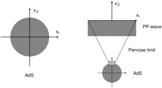
Figure 1: AdS, pp-wave and Penrose limit.

3 Penrose Limit of $z$ for AdS${}_{5}\times$S⁵

To begin with, we shall consider the Penrose limit of the function $z$ for the AdS${}_{5}\times$S⁵ case:

$$\tilde{z}(r,y;r_{0})=\frac{r^{2}-r^{2}_{0}+y^{2}}{2\sqrt{(r^{2}+r^{2}_{0}+y^{2})^{2}-4r^{2}r^{2}_{0}}}-\frac{1}{2}\,.$$ (3.1)

The coordinate system of the LLM background for this $z$ is different from the standard global coordinates of the AdS${}_{5}\times$S⁵ background. In order to obtain the standard expression of the AdS${}_{5}\times$S⁵ we need to perform the change of coordinates as follows:

$$y=r_{0}\sinh\rho\,\sin\theta\,,\quad r=r_{0}\cosh\rho\,\cos\theta\,,\quad\widetilde{\phi}=\phi-t\,.$$ (3.2)

Here the radius $r_{0}$ is identified with the AdS radius $R$ via $r_{0}=R^{2}$ .

Let us recall how to take the Penrose limit in the metric. The AdS${}_{5}\times$S⁵ metric with global coordinates is given by

$$ds^{2}=R^{2}\left[-\cosh^{2}\rho\,dt^{2}+d\rho^{2}+\sinh^{2}\,\rho d\Omega_{3}^{2}+\cos^{2}\theta\,d\widetilde{\phi}^{2}+d\theta^{2}+\sin^{2}\theta\,d\widetilde{\Omega}_{3}^{2}\right]\,.$$ (3.3)

Here we introduce the following parameterization utilized by Callan et.al [19]:

$$\cosh\rho=\frac{1+r_{1}^{2}/4}{1-r_{1}^{2}/4}\,,\qquad\cos\theta=\frac{1-r^{2}_{2}/4}{1+r^{2}_{2}/4}\,.$$ (3.4)

When we will take a limit $R\rightarrow\infty$ by rescaling $r_{1}$ and $r_{2}$ as $r_{1}\rightarrow r_{1}/R$ and $r_{2}\rightarrow r_{2}/R$, respectively, the resulting function $z$ , up to and including $1/R^{2}$ , is

$$z=\frac{r_{1}^{2}-r_{2}^{2}}{2(r_{1}^{2}+r_{2}^{2})}+\frac{r_{1}^{2}r_{2}^{2}}{2(r_{1}^{2}+r_{2}^{2})}\frac{1}{R^{2}}+\mathcal{O}(1/R^{4})\,.$$ (3.5)

In order to obtain the function $z$ in terms of $x_{1},x_{2},y$ , we need to perform a coordinate transformation from $(r_{1},r_{2})$ to $(r,y)$ . In course of the calculation $1/R^{2}$ corrections appear and so we have to be careful to do it.

We firstly expand $y$ and $r$ with respect to $r_{1}$ and $r_{2}$ (after the rescaling) as

$$y=r_{1}r_{2}+\frac{1}{4R^{2}}r_{1}r_{2}(r_{1}^{2}-r_{2}^{2})+\mathcal{O}(1/R^{4})\,,$$ (3.6)

$$r=r_{0}+\frac{1}{2}(r_{1}^{2}-r^{2}_{2})+\frac{r_{0}}{8R^{2}}(r_{1}^{2}-r_{2}^{2})^{2}+\mathcal{O}(1/R^{4})\,.$$ (3.7)

From (3.6) and (3.7) we obtain

$$\frac{1}{2R^{2}}(r_{1}^{2}-r_{2}^{2})=-1\pm\sqrt{\frac{2r}{r_{0}}-1}\,,\qquad r_{1}r_{2}=\frac{2y}{1\pm\sqrt{\frac{2r}{r_{0}}-1}}\,.$$ (3.8)

We have two choices to take a pair of $r_{1}$ and $r_{2}$ due to the sign $\pm$ that appears when we solved the quadratic algebraic equation (3.7) . But we should choose the “$+$” sign that leads to $y=r_{1}r_{2}$ at the zero-th order of $1/R^{2}$ . The relation $y=r_{1}r_{2}$ is utilized in [7]. By using (3.8) we can rewrite the first term in (3.5) as

$$\frac{r_{1}^{2}-r^{2}_{2}}{2(r_{1}^{2}+r_{2}^{2})}=\frac{r-r_{0}}{2\sqrt{\left(r-r_{0}\right)^{2}+y^{2}}}\,.$$ (3.9)

Now let us introduce a new variable $x_{2}^{\prime}=x_{2}-r_{0}$ . This shift of $x_{2}$ corresponds to that of the origin in the 2-plane. That is, the origin in the system of coordinates for the AdS is shifted to the north-pole of the disk, and the resulting origin is nothing but the origin in 2-plane for the pp-wave (see Fig. 1). Then it is possible to expand $r^{2}=x_{1}^{2}+x_{2}^{2}$ as

$$r=\sqrt{x_{1}^{2}+(x_{2}^{\prime}+r_{0})^{2}}=(x_{2}^{\prime}+r_{0})+\frac{x_{1}^{2}}{2(x_{2}^{\prime}+r_{0})}+\cdots\,.$$ (3.10)

By using (3.10), we can express the first term in (3.5) in terms of $(x_{1},x^{\prime}_{2})$:

$$\frac{r_{1}^{2}-r_{2}^{2}}{2(r_{1}^{2}+r_{2}^{2})}=\frac{x_{2}^{\prime}}{2\sqrt{x_{2}^{\prime}{}^{2}+y^{2}}}+\frac{x_{1}^{2}\,y^{2}}{4R^{2}(x_{2}^{\prime}{}^{2}+y^{2})^{3/2}}+\mathcal{O}(1/R^{4})\,.$$ (3.11)

Thus the first term in (3.5) has been decomposed into the leading term and the sub-leading term. As a matter of course, the leading term agrees with the result of LLM [7].

In order to finish evaluating the $1/R^{2}$-corrections it is necessary to investigate the second term in (3.5) . It is easy to show that

$$\frac{r_{1}^{2}r_{2}^{2}}{2R^{2}(r_{1}^{2}+r_{2}^{2})}=\frac{y^{2}}{4R^{2}\sqrt{x_{2}^{\prime}{}^{2}+y^{2}}}+\mathcal{O}(1/R^{4})\,,$$ (3.12)

and so the resulting function $z$ with $1/R^{2}$ contributions is given by

$$z(x_{1},x_{2}^{\prime},y)=\frac{r_{1}^{2}-r_{2}^{2}}{2(r_{1}^{2}+r_{2}^{2})}+\frac{r_{1}^{2}r_{2}^{2}}{2(r_{1}^{2}+r_{2}^{2})}\frac{1}{R^{2}}+\mathcal{O}(1/R^{4})$$

$$\qquad\qquad~{}~{}=\frac{x_{2}^{\prime}}{2\sqrt{x_{2}^{\prime}{}^{2}+y^{2}}}+\frac{1}{4R^{2}}\left[\frac{x_{1}^{2}\,y^{2}}{(x_{2}^{\prime}{}^{2}+y^{2})^{3/2}}+\frac{y^{2}}{\sqrt{x_{2}^{\prime}{}^{2}+y^{2}}}\right]+\mathcal{O}(1/R^{4})\,.$$ (3.13)

It is an easy task to show directly that the function $z$ given in (3.13) satisfies the differential equation (2.3) . Hence the pp-wave with $1/R^{2}$ terms may be contained in the context of bubbling 1/2 BPS geometries.

We shall next consider the Penrose limit of the $V_{r}$ and $V_{\phi}$ for the AdS:

$$V_{r}=0\,,\qquad V_{\phi}=-\frac{1}{2}\left(\frac{r^{2}+r_{0}^{2}+y^{2}}{\sqrt{(r^{2}+r^{2}_{0}+y^{2})^{2}-4r^{2}r^{2}_{0}}}-1\right)\,.$$ (3.14)

For the pp-wave case the Cartesian coordinates $(x_{1},x_{2})$ are more suitable than the polar coordinates $(r,\phi)$ since the droplet configuration is the lower-half plane rather than a disk. Through the coordinate transformations we can find the following $V_{1}$ and $V_{2}$ for the pp-wave with $1/R^{2}$ terms:

$$V_{1}=\frac{\partial\phi}{\partial x_{1}}V_{\phi}+\frac{\partial r}{\partial x_{1}}V_{r}=-\frac{\sin\phi}{r}V_{\phi}=-\frac{x^{\prime}_{2}+r_{0}^{2}}{x_{1}^{2}+(x^{\prime}_{2}+r_{0})^{2}}V_{\phi}$$

$$\quad\,\,=\frac{1}{2\sqrt{x^{\prime}_{2}{}^{2}+y^{2}}}-\frac{1}{R^{2}}\left[\frac{1}{2}+\frac{x^{\prime}_{2}(x_{1}^{2}+x^{\prime}_{2}{}^{2}+y^{2})}{4(x^{\prime}_{2}{}^{2}+y^{2})^{3/2}}\right]+\mathcal{O}(1/R^{4})$$ (3.15)

$$\quad\,\,=\frac{1}{r_{1}^{2}+r_{2}^{2}}-\frac{r_{1}^{2}}{R^{2}(r_{1}^{2}+r_{2}^{2})}+\mathcal{O}(1/R^{4})\,,$$

$$V_{2}=\frac{\partial\phi}{\partial x_{2}}V_{\phi}+\frac{\partial r}{\partial x_{2}}V_{r}=\frac{\cos\phi}{r}V_{\phi}=\frac{x_{1}}{x_{1}^{2}+(x^{\prime}_{2}+r_{0})^{2}}V_{\phi}$$

$$\quad\,\,=-\frac{x_{1}}{2R^{2}\sqrt{x^{\prime}_{2}{}^{2}+y^{2}}}+\mathcal{O}(1/R^{4})=-\frac{x_{1}}{R^{2}(r_{1}^{2}+r_{2}^{2})}+\mathcal{O}(1/R^{4})\,.$$ (3.16)

The above $V_{1}$ and $V_{2}$ satisfy the differential equations (2.2) with the function $z$ given in (3.13) . As a remark, the constant term $1/2R^{2}$ in the expression of $V_{1}$ (3.15) would not be determined by solving the differential equation but it is properly determined by carefully considering the Penrose limit. It is also worth remaking that the relation $z=x_{2}^{\prime}V_{1}-x_{1}V_{2}$, mentioned in [10], begins to fail at the $1/R^{2}$-order:

$$x_{2}^{\prime}V_{1}-x_{1}V_{2} = \frac{{x_{2}^{\prime}}}{2{\sqrt{y^{2}+{{x_{2}^{\prime}}}^{2}}}}-\frac{1}{4R^{2}}\Bigg{[}{2{x_{2}^{\prime}}+\frac{{{x_{2}^{\prime}}}^{2}\left(y^{2}+{{x_{2}^{\prime}}}^{2}\right)-{{x_{1}}}^{2}\left(2y^{2}+{{x_{2}^{\prime}}}^{2}\right)}{{\left(y^{2}+{{x_{2}^{\prime}}}^{2}\right)}^{\frac{3}{2}}}}\Bigg{]}+{\cal O}(1/R^{4})\,.$$

By putting the functions (3.13), (3.15) and (3.16) into the metric (2.1), we can derive the metric:

$$ds^{2}=-2dtdx_{1}-(r_{1}^{2}+r_{2}^{2})dt^{2}+d\vec{r_{1}}^{2}+d\vec{r_{2}}^{2}$$ (3.17)

$$\qquad\qquad+\frac{1}{R^{2}}\Bigl{[}dx_{1}^{2}+\frac{1}{2}(r_{1}^{2}d\vec{r_{1}}^{2}-r_{2}^{2}d\vec{r_{2}}^{2})+\frac{1}{2}(r_{2}^{4}-r_{1}^{4})dt^{2}$$

$$\qquad\qquad+dtdx_{1}(r_{1}^{2}+r_{2}^{2})+2x_{1}(r_{1}dr_{1}dt-r_{2}dr_{2}dt)\Bigr{]}+\mathcal{O}(1/R^{4})\,,$$

where we have written down the metric in terms of the coordinates $(r_{1},r_{2})$ rather than $(y,x_{2})$ . We also used the following expansions of $y{\rm e}^{G}$ and $y{\rm e}^{-G}$ :

$$y{\rm e}^{G}=\frac{y^{2}}{-x^{\prime}_{2}+\sqrt{x^{\prime}_{2}{}^{2}+y^{2}}}+\frac{y^{2}(x_{1}^{2}+x^{\prime}_{2}{}^{2}+y^{2})}{2R^{2}(x^{\prime}_{2}{}^{2}+y^{2}-x^{\prime}_{2}\sqrt{x^{\prime}_{2}{}^{2}+y^{2}})}+\mathcal{O}(1/R^{4})$$

$$\qquad=r_{1}^{2}+\frac{r_{1}^{4}}{2R^{2}}+\mathcal{O}(1/R^{4})\,,$$

$$y{\rm e}^{-G}=-x^{\prime}_{2}+\sqrt{x^{\prime}_{2}{}^{2}+y^{2}}-\frac{(x_{1}^{2}+x^{\prime}_{2}{}^{2}+y^{2})\left(x^{\prime}_{2}{}^{2}+y^{2}-x^{\prime}_{2}\sqrt{x^{\prime}_{2}{}^{2}+y^{2}}\right)}{2R^{2}(x^{\prime}_{2}{}^{2}+y^{2})}+\mathcal{O}(1/R^{4})$$

$$\qquad\,\,\,=r_{2}^{2}-\frac{r_{2}^{4}}{2R^{2}}+\mathcal{O}(1/R^{4})\,.$$

Furthermore performing the shift of $x_{1}$  as $x_{1}=x^{\prime}_{1}+x^{\prime}_{1}x_{2}^{\prime}/R^{2}\,,$ and identifying as $t\equiv x^{+}$ and $x^{\prime}_{1}\equiv-x^{-}$ gives the pp-wave metric with $1/R^{2}$ corrections considered in [19]:

$$ds^{2}=2dx^{+}dx^{-}+d\vec{r_{1}}^{2}+d\vec{r_{2}}^{2}-(r_{1}^{2}+r_{2}^{2})(dx^{+})^{2}$$ (3.18)

$$\quad~{}+\frac{1}{R^{2}}\left[-2y^{2}dx^{-}dx^{+}+\frac{1}{2}(r_{2}^{4}-r_{1}^{4})(dx^{+})^{2}+(dx^{-})^{2}+\frac{1}{2}r_{1}^{2}d\vec{r_{1}}^{2}-\frac{1}{2}r_{2}^{2}d\vec{r_{2}}^{2}\right]+\mathcal{O}\left(1/R^{4}\right)\,.$$

Here the convention of the light-cone coordinates is absorbed into the identification between $x^{-}$ and $x^{\prime}_{1}$ . As an additional remark, the shift of $x_{1}$ does not change the expression of $z$, $V_{1}$, and $V_{2}$ at the order of $1/R^{2}$ .

Finally we should note that the function $z$ including the $1/R^{2}$-corrections has the same boundary condition at $y=0$ as in the case of $z$ without $1/R^{2}$-corrections, although the $V_{2}$ becomes non-zero due to the $1/R^{2}$-correction. That is, $1/R^{2}$-corrections are irrelevant to the droplet.

4 Higher Order $1/R^{2}$-Corrections

In this section we further investigate higher order $1/R^{2}$-corrections at the order of $1/R^{6}$ . Using the relation (3.10) found in the section 3, the higher order $1/R^{2}$-corrections of the $z$ can be computed as

$$z(x_{1},x_{2}^{\prime},y) = \frac{x_{2}^{\prime}}{2\,{\sqrt{{x_{2}^{\prime}}^{2}+y^{2}}}}+\frac{y^{2}\,\left({x_{2}^{\prime}}^{2}+y^{2}+{{x_{1}}}^{2}\right)}{4\,R^{2}\,{\left({x_{2}^{\prime}}^{2}+y^{2}\right)}^{\frac{3}{2}}}-\frac{3\,x_{2}^{\prime}\,y^{2}\,{\left({x_{2}^{\prime}}^{2}+y^{2}+{{x_{1}}}^{2}\right)}^{2}}{16\,R^{4}\,{\left({x_{2}^{\prime}}^{2}+y^{2}\right)}^{\frac{5}{2}}}$$ (4.1)

$$\quad-\frac{y^{2}\,\left(y^{2}-4\,x_{2}^{\prime 2}\right)\,{\left(y^{2}+{{x_{1}}}^{2}+x_{2}^{\prime 2}\right)}^{3}}{32\,R^{6}\,{\left(y^{2}+x_{2}^{\prime 2}\right)}^{\frac{7}{2}}}+{\cal O}(1/R^{8}).$$

We can explicitly check that the function $z$ obeys the differential equation (2.3). It is worth while noting that the droplet configuration $z(x_{1},x_{2}^{\prime},y=0)$ of (4.1) is the same as the pp-wave one (the right hand side in Fig. 1) even at the order of $1/R^{6}$. Hence it is expected that the droplet configuration would be the same as the pp-wave one even if we include any finite $1/R^{2}$-corrections. As a matter of course, when we include all order $1/R^{2}$-corrections, the droplet configuration would become the AdS₅$\times$S⁵ one (the left hand side in Fig. 1). One possible reason why the different geometries give the same droplet configuration is that the size of the droplet for the pp-wave is infinite in comparison to the finite size droplet for the AdS case. Hence it might be necessary to give more boundary conditions at infinity as in the argument given in the case of pp-wave (with no corrections) [7], when we consider the $1/R^{2}$-corrections. Another possible explanation is that the two limits $R\to\infty$ and $y\to 0$ do not commute. When we first take the limit $R\to\infty$, the droplet boundary goes to infinity. This limit would hide the behavior of $z$ near the boundaries at infinity. Then the limit of $y\to 0$ would give the same droplet configuration as the one without $1/R^{2}$-corrections.

In order to obtain $z$ as a function of $(r_{1},r_{2},x_{1})$ we expand $y$ and $x_{2}^{\prime}$ in terms of $r_{1}$ and $r_{2}$,

$$y = r_{1}r_{2}+\frac{r_{1}r_{2}}{4R^{2}}(r_{1}^{2}-r_{2}^{2})+\frac{{r_{1}}{r_{2}}}{16R^{4}}\left(r_{1}^{4}-r_{1}^{2}r_{2}^{2}+r_{2}^{4}\right)+\frac{r_{1}r_{2}}{64R^{6}}\left(r_{1}^{2}-r_{2}^{2}\right)\left(r_{1}^{4}+r_{2}^{4}\right)+{\cal O}(1/R^{8}),$$

$$x_{2}^{\prime} = \frac{1}{2}(r_{1}^{2}-r_{2}^{2})+\frac{1}{8R^{2}}[(r_{1}^{2}-r_{2}^{2})^{2}-4x_{1}^{2}]+\frac{r_{1}^{2}-r_{2}^{2}}{32R^{4}}\left({{r_{1}}}^{4}-{{r_{1}}}^{2}{{r_{2}}}^{2}+{{r_{2}}}^{4}+8{{x_{1}}}^{2}\right)$$

$$+\frac{{\left({{r_{1}}}^{2}-{{r_{2}}}^{2}\right)}^{2}\left({{r_{1}}}^{4}+{{r_{2}}}^{4}\right)-8{\left({{r_{1}}}^{2}-{{r_{2}}}^{2}\right)}^{2}{{x_{1}}}^{2}-16{{x_{1}}}^{4}}{128R^{6}}+{\cal O}(1/R^{8}).$$

By using these relations, we can rewrite (4.1) in terms of $r_{1}$ and $r_{2}$ as follows:

$$z=\frac{r_{1}^{2}-r_{2}^{2}}{2(r_{1}^{2}+r_{2}^{2})}+\frac{r_{1}^{2}r_{2}^{2}}{2R^{2}(r_{1}^{2}+r_{2}^{2})}+\frac{r_{1}^{2}r_{2}^{4}-r_{1}^{4}r_{2}^{2}}{16R^{4}\left(r_{1}^{2}+r_{2}^{2}\right)}-\frac{r_{1}^{4}r_{2}^{4}}{32R^{6}\left(r_{1}^{2}+r_{2}^{2}\right)}+{\cal O}(1/R^{8}).$$ (4.2)

In order to obtain the metric including the $1/R^{6}$-corrections we compute $V_{1}$, $V_{2}$, $ye^{G}$ and $ye^{-G}$ in terms of $x_{1}$, $r_{1}$ and $r_{2}$. The results for $V_{1}$ and $V_{2}$ are

$$V_{1} = \frac{1}{2{\sqrt{y^{2}+x_{2}^{\prime 2}}}}-\frac{{x_{2}^{\prime}}\left(y^{2}+x_{1}^{2}+{x_{2}^{\prime}}^{2}\right)}{4{(y^{2}+{{x_{2}^{\prime}}}^{2})}^{{3}/{2}}R^{2}}-\frac{1}{2R^{2}}+\frac{x_{2}^{\prime}}{2R^{4}}$$

$$+\frac{1}{16R^{4}{({x_{2}^{\prime}}^{2}+y^{2})}^{5/2}}\left[{{({x_{2}^{\prime}}^{2}+y^{2})}^{2}(6{x_{2}^{\prime}}^{2}+3y^{2})-6y^{2}({x_{2}^{\prime}}^{2}+y^{2}){{x_{1}}}^{2}+(2{x_{2}^{\prime}}^{2}-y^{2})x_{1}^{4}}\right]$$

$$+\frac{1}{32R^{6}(y^{2}+{x_{2}^{\prime}}^{2})^{4}}\bigg{\{}-x_{2}^{\prime}\sqrt{y^{2}+x_{2}^{\prime 2}}\bigg{[}x_{1}^{4}(y^{2}+{x_{2}^{\prime}}^{2})(-13y^{2}+2{{x_{2}^{\prime}}}^{2})+x_{1}^{6}(-3y^{2}+2{x_{2}^{\prime}}^{2})$$

$$\quad-3x_{1}^{2}(y^{2}+{{x_{2}^{\prime}}}^{2})^{2}(11y^{2}+6{x_{2}^{\prime}}^{2})+(y^{2}+{x_{2}^{\prime}}^{2})^{3}(9y^{2}+14{x_{2}^{\prime}}^{2})\bigg{]}\bigg{\}}+\frac{x_{1}^{2}-{x_{2}^{\prime}}^{2}}{2R^{6}}+{\cal O}(1/R^{8})$$

$$= \frac{1}{r_{1}^{2}+r_{2}^{2}}-\frac{r_{1}^{2}}{R^{2}(r_{1}^{2}+r_{2}^{2})}-\frac{r_{2}^{4}+r_{1}^{2}r_{2}^{2}-7r_{1}^{4}+8x_{1}^{2}}{16R^{4}(r_{1}^{2}+r_{2}^{2})}+\frac{r_{1}^{2}(16x_{1}^{2}-2r_{1}^{4}+r_{2}^{4})-r_{2}^{2}(8x_{1}^{2}-r_{1}^{4})}{16R^{6}(r_{1}^{2}+r_{2}^{2})}$$

$$+{\cal O}(1/R^{8}),$$

$$V_{2} = -\frac{{x_{1}}}{2R^{2}{\sqrt{y^{2}+x_{2}^{\prime 2}}}}+\frac{x_{1}x_{2}^{\prime}}{4R^{4}}\frac{x_{1}^{2}+3({x_{2}^{\prime}}^{2}+y^{2})}{{(x_{2}^{\prime 2}+y^{2})}^{{3}/{2}}}+\frac{x_{1}}{2R^{4}}-\frac{x_{2}^{\prime}}{R^{6}}$$

$$\quad+\frac{x_{1}\left\{x_{1}^{4}(y^{2}-2x_{2}^{\prime 2})-3(y^{2}+x_{2}^{\prime 2})^{2}(y^{2}+6x_{2}^{\prime 2})+x_{1}^{2}(6y^{4}+2y^{2}x_{2}^{\prime 2}-4x_{2}^{\prime 4})\right\}}{16R^{6}{\left(y^{2}+{{x_{2}^{\prime}}}^{2}\right)}^{\frac{5}{2}}}+{\cal O}(1/R^{8})$$

$$= -\frac{{x_{1}}}{R^{2}\left({{r_{1}}}^{2}+{{r_{2}}}^{2}\right)}+\frac{\left(3{{r_{1}}}^{2}-{{r_{2}}}^{2}\right){x_{1}}}{2R^{4}\left({{r_{1}}}^{2}+{{r_{2}}}^{2}\right)}-\frac{\left(17{{r_{1}}}^{4}-13{{r_{1}}}^{2}{{r_{2}}}^{2}+{{r_{2}}}^{4}\right){x_{1}}}{16R^{6}\left({{r_{1}}}^{2}+{{r_{2}}}^{2}\right)}+{\cal O}(1/R^{8}).$$

We can check that $V_{1}$ and $V_{2}$ obey the equations (2.2). It is worth noting again that the $y$-independent terms in (4) and (4) would not be completely determined from the differential equations (2.2), although they constrain the relation between the undetermined terms in $V_{1}$ and the ones in $V_{2}$.

Using Eq. (4.2) the results for $ye^{G}$ and $ye^{-G}$ are

$$ye^{G} = r_{1}^{2}+\frac{r_{1}^{4}}{2R^{2}}+\frac{3r_{1}^{6}}{16R^{4}}+\frac{r_{1}^{8}}{16R^{6}}+{\cal O}(1/R^{8}),$$

$$ye^{-G} = r_{2}^{2}-\frac{r_{2}^{4}}{2R^{2}}+\frac{3r_{2}^{6}}{16R^{4}}-\frac{r_{2}^{8}}{16R^{6}}+{\cal O}(1/R^{8}).$$

Thus the resulting metric is

$$ds^{2} = 2dx^{+}dx^{-}-(r_{1}^{2}+r_{2}^{2})(dx^{+})^{2}+d\vec{r}_{1}{}^{2}+d\vec{r}_{2}{}^{2}$$

$$+\frac{1}{R^{2}}\bigg{[}2r_{2}^{2}dx^{+}dx^{-}+(dx^{-})^{2}-(r_{1}^{4}-r_{2}^{4})(dx^{+})^{2}+\frac{1}{2}r_{1}^{2}d\vec{r}_{1}{}^{2}-\frac{1}{2}r_{2}^{2}d\vec{r}_{2}{}^{2}\bigg{]}$$

$$+\frac{1}{R^{4}}\bigg{[}-r_{2}^{4}dx^{+}dx^{-}-r_{2}^{2}(dx^{-})^{2}-\frac{3}{16}(r_{1}^{6}+r_{2}^{6})(dx^{+})^{2}+\frac{3}{16}r_{1}^{4}{{{{d\vec{r}}}_{1}}}^{2}+\frac{3}{16}r_{2}^{4}{{{{d\vec{r}}}_{2}}}^{2}\bigg{]}$$

$$+\frac{1}{16R^{6}}\bigg{[}6r_{2}^{6}dx^{+}dx^{-}+8r_{2}^{4}(dx^{-})^{2}-(r_{1}^{8}-r_{2}^{8})(dx^{+})^{2}+r_{1}^{6}{{{{d\vec{r}}}_{1}}}^{2}-r_{2}^{6}{{{{d\vec{r}}}_{2}}}^{2}\bigg{]}+{\cal O}(1/R^{8})$$

where we have used the coordinate-transformation from $x_{1}$ to $x_{1}^{\prime}$ defined as

$$x_{1} \equiv x_{1}^{\prime}+\frac{x_{1}^{\prime}x_{2}^{\prime}}{R^{2}}+\frac{x_{1}^{\prime}{}^{3}}{2R^{4}}+\frac{x_{1}^{\prime}{}^{3}x_{2}^{\prime}}{3R^{6}}+{\cal O}(1/R^{8})$$

$$= x_{1}^{\prime}+\frac{x_{1}^{\prime}(r_{1}^{2}-r_{2}^{2})}{2R^{2}}-\frac{x_{1}^{\prime 3}}{6R^{4}}+\frac{x_{1}^{\prime}}{8R^{4}}(r_{1}^{2}-r_{2}^{2})^{2}-\frac{{x_{1}^{\prime}}^{3}(r_{1}^{2}-r_{2}^{2})}{12R^{6}}+\frac{x_{1}^{\prime}(r_{1}^{2}-r_{2}^{2})}{32R^{6}}\left[r_{1}^{4}-r_{1}^{2}r_{2}^{2}+r_{2}^{4}\right]$$

$$\quad+{\cal O}(1/R^{8}),$$

and the same identifications in section 3 : $t\equiv x^{+}$ and $x_{1}^{\prime}\equiv-x^{-}$  .

5 Concentric Rings

As a simple extension of the discussion in section 3, let us consider the geometry characterized by a family of concentric rings [7] (see Fig. 3). This solution is given by the following $z,V_{r},V_{\phi}$:

$$\tilde{z}=\frac{1}{2}\sum_{n=1}^{N}(-1)^{n+1}\left(\frac{r^{2}-r^{2}_{n}+y^{2}}{\sqrt{(r^{2}+r^{2}_{n}+y^{2})^{2}-4r^{2}r^{2}_{n}}}-1\right)\,,$$

$$V_{r}=0\,,\quad V_{\phi}=\frac{1}{2}\sum_{n=1}^{N}(-1)^{n}\left(\frac{r^{2}+r^{2}_{n}+y^{2}}{\sqrt{(r^{2}+r^{2}_{n}+y^{2})^{2}-4r^{2}r^{2}_{n}}}-1\right)\,,$$

where we have used the polar coordinates $(r,\phi)$ instead of $(x_{1},x_{2})$ . The $r_{1}$ is the radius of the outermost circle, $r_{2}$ the next one and so on. This background is time-independent and in certain limits can be thought of as a configuration of smeared S⁵ giants and/or their AdS₅ duals.

It is easy to apply the previous analysis to this case. All we have to do is to introduce the shifts of variables as follows:

$$x_{2}-r_{n}=(x_{2}-r_{0})-(r_{n}-r_{0})\equiv x^{\prime}_{2}-x_{2}^{(n)}\,.$$ (5.1)

Then the radius coordinate $r$ is expanded as

$$r=\sqrt{x_{1}^{2}+(x_{2}^{\prime}-x_{2}^{(n)}+r_{n})^{2}}=(x_{2}^{\prime}-x_{2}^{(n)}+r_{n})+\frac{x_{1}^{2}}{2(x_{2}^{\prime}-x_{2}^{(n)}+r_{n})}+\cdots\,.$$ (5.2)

In addition we assume that $r_{0}$ is much bigger than $x_{2}^{(n)}$ (thin ring approximation) and expand $r_{n}$ as

$$r_{n}=r_{0}\left(1+\frac{x_{2}^{(n)}}{r_{0}}\right)\equiv r_{0}\left(1+\epsilon^{(n)}\right)\,.$$

The remaining part of the analysis is similar to that in the AdS${}_{5}\times$S⁵ ($N=1$ case) and the $1/R^{2}$ corrections in this case can be also evaluated. The resulting function $z$ after taking the Penrose limit in the configuration of the concentric rings is

$$z=\frac{1}{2}\sum_{n=1}^{N}(-1)^{n+1}\left\{\frac{x^{\prime}_{2}-x_{2}^{(n)}}{\sqrt{(x^{\prime}_{2}-x_{2}^{(n)})^{2}+y^{2}}}+\frac{y^{2}\left[(x^{\prime}_{2}-x_{2}^{(n)})^{2}+x_{1}^{2}+y^{2}\right]}{2R^{2}\left[(x^{\prime}_{2}-x_{2}^{(n)})^{2}+y^{2}\right]^{3/2}}\right\}+\mathcal{O}(1/R^{4})\,.$$ (5.3)

Then $V_{1}$ and $V_{2}$ are given by

$$V_{1}=\sum_{n=1}^{N}(-1)^{n-1}\Biggl{\{}\frac{1}{2\sqrt{(x^{\prime}_{2}-x_{2}^{(n)})^{2}+y^{2}}}$$ (5.4)

$$\hskip 93.89418pt-\frac{1}{R^{2}}\Biggl{[}\frac{1}{2}+\frac{(x^{\prime}_{2}-x_{2}^{(n)})\bigl{[}x_{1}^{2}+(x^{\prime}_{2}-x_{2}^{(n)})^{2}+y^{2}\bigr{]}}{4\bigl{[}(x^{\prime}_{2}-x_{2}^{(n)})^{2}+y^{2}\bigr{]}^{3/2}}\Biggr{]}\Biggr{\}}+\mathcal{O}(1/R^{4})\,,$$

$$V_{2}=\sum_{n=1}^{N}(-1)^{n}\frac{x_{1}}{2R^{2}\sqrt{(x^{\prime}_{2}-x_{2}^{(n)})^{2}+y^{2}}}+\mathcal{O}(1/R^{4})\,.$$ (5.5)

The droplet configurations at $y=0$ are a set of stripes as noted by LLM [7] (see Fig. 3). The leading part of the above result agrees with the one in [14]. We have plotted two graphs (Figs. 3 and 3) by using the contour plot in the Mathematica with the data: $r_{1}=R^{2},~{}r_{2}=0.99R^{2},~{}r_{3}=0.96R^{2},~{}r_{4}=0.95R^{2},~{}r_{5}=0.92R^{2},~{}r_{6}=0.91R^{2},~{}r_{7}=0.6R^{2},~{}R=2$ . Our result (5.3) surely reproduces a set of strips from the concentric rings via the Penrose limit.

Figure 2: Configuration of concentric rings. Figure 3: Penrose limit of concentric rings.

In a similar way we can compute the higher order corrections for concentric rings.

6 A Conclusion and Discussions

We have discussed how to take a Penrose limit in bubbling 1/2 BPS geometries at the stage of a single function $z(x_{1},x_{2},y)$ . Taking the Penrose limit for the function $z$ for the AdS, we can directly obtain the $z$ for the pp-wave with $1/R^{2}$-corrections. It satisfies the differential equation and leads to the pp-wave metric with $1/R^{2}$-corrections. In particular, our result reproduces the pp-wave metric used in [19].

It should be however noted that the function with $1/R^{2}$-corrections has the same boundary condition at $y=0$ as the $z$ without the corrections. Hence the $1/R^{2}$-corrections are not determined by naively imposing a boundary condition at $y=0$ , and it would be necessary to take more careful treatments. But, by considering the Penrose limit at the stage of the single function $z$ for the AdS space (or metrics of other spacetimes), it is possible to properly take $1/R^{2}$-corrections into account in bubbling 1/2 BPS geometries.

We also considered the higher $1/R^{2}$-contributions to the $z$ . We saw that higher-order corrections do not modify the half-filling configuration as well as the second order corrections. That is, the $z$ has the same boundary condition at $y=0$ as the $z$ with no correction. One possible reason why the different geometries give the same droplet configuration is that the size of the droplet for the pp-wave is infinite in comparison to the finite size droplet for the AdS case. It might be necessary to give more boundary conditions at infinity as in the argument given in the case of pp-wave (with no corrections) [7], when we consider the $1/R^{2}$-corrections. It was also found that the $y$-independent terms in $V_{1}$ and $V_{2}$ would not be completely determined from the differential equations (2.2), although they constrain the relation between the undetermined terms in $V_{1}$ and the ones in $V_{2}$ . It would be nice to apply our discussion to other metrics (for example, [11]) and derive the corresponding function $z$ (with $1/R^{2}$-corrections). On the other hand, it is interesting to consider the description of $1/R^{2}$-corrections in terms of the free fermion in the SYM side. In this direction it would be valuable to comment on the work of Horava and Shepard [10]. They also considered the Penrose limit of LLM geometries, and in particular, showed that the Penrose limit towards the (nearly) singular null geodesic of the geometry (nearly) at topological transition is equivalent to the well-known double-scaling limit of the matrix model that defines two-dimensional noncritical string theory (in fact, the Type 0 version of it [20], since both sides of the Fermi sea are filled). Hence the $1/R^{2}$-corrections in the Penrose limit would correspond to the corrections to the double scaled matrix model. It is also worthwhile to say that the non-relativistic free fermions would become relativistic in the Penrose limit according to the LLM’s observation [7]. Then it would be expected that the $1/R^{2}$-corrections interpolate between the non-relativistic fermions and relativistic ones in the Penrose limit.

References

• [1] J. M. Maldacena, “The large N limit of superconformal field theories and supergravity,” Adv. Theor. Math. Phys.  2 (1998) 231 [Int. J. Theor. Phys.  38 (1999) 1113] [arXiv:hep-th/9711200]; S. S. Gubser, I. R. Klebanov and A. M. Polyakov, “Gauge theory correlators from non-critical string theory,” Phys. Lett. B 428 (1998) 105 [arXiv:hep-th/9802109]; E. Witten, “Anti-de Sitter space and holography,” Adv. Theor. Math. Phys.  2 (1998) 253 [arXiv:hep-th/9802150].
• [2] J. McGreevy, L. Susskind and N. Toumbas, “Invasion of the giant gravitons from anti-de Sitter space,” JHEP 0006 (2000) 008 [arXiv:hep-th/0003075].
• [3] M. T. Grisaru, R. C. Myers and O. Tafjord, “SUSY and Goliath,” JHEP 0008 (2000) 040 [arXiv:hep-th/0008015].
A. Hashimoto, S. Hirano and N. Itzhaki, “Large branes in AdS and their field theory dual,” JHEP 0008 (2000) 051 [arXiv:hep-th/0008016].
• [4] S. Corley, A. Jevicki and S. Ramgoolam, “Exact correlators of giant gravitons from dual N = 4 SYM theory,” Adv. Theor. Math. Phys.  5 (2002) 809 [arXiv:hep-th/0111222].
The description of particles and holes in this reference is given in the c=1 context in, A. Jevicki, “Nonperturbative collective field theory,” Nucl. Phys. B 376 (1992) 75.
• [5] D. Berenstein, “A toy model for the AdS/CFT correspondence,” JHEP 0407 (2004) 018 [arXiv:hep-th/0403110].
• [6] M. M. Caldarelli and P. J. Silva, “Giant gravitons in AdS/CFT. I: Matrix model and back reaction,” JHEP 0408 (2004) 029 [arXiv:hep-th/0406096].
• [7] H. Lin, O. Lunin and J. Maldacena, “Bubbling AdS space and 1/2 BPS geometries,” JHEP 0410 (2004) 025 [arXiv:hep-th/0409174].
• [8] M. M. Caldarelli, D. Klemm and P. J. Silva, “Chronology protection in anti-de Sitter,” arXiv:hep-th/0411203.
• [9] G. Mandal, “Fermions from half-BPS supergravity,” arXiv:hep-th/0502104.
• [10] P. Horava and P. G. Shepard, “Topology changing transitions in bubbling geometries,” arXiv:hep-th/0502127.
• [11] J. T. Liu, D. Vaman and W. Y. Wen, “Bubbling 1/4 BPS solutions in type IIB and supergravity reductions on Sn$\times$Sn,” arXiv:hep-th/0412043.
D. Martelli and J. F. Morales, “Bubbling AdS3,” arXiv:hep-th/0412136.
N. V. Suryanarayana, “Half-BPS giants, free fermions and microstates of superstars,” arXiv:hep-th/0411145.
Z. W. Chong, H. Lu and C. N. Pope, “BPS geometries and AdS bubbles,” arXiv:hep-th/0412221.
J. T. Liu and D. Vaman, “Bubbling 1/2 BPS solutions of minimal six-dimensional supergravity,” arXiv:hep-th/0412242.
O. Lunin and J. Maldacena, “Deforming field theories with U(1)$\times$U(1) global symmetry and their gravity duals,” arXiv:hep-th/0502086.
• [12] S. S. Gubser, I. R. Klebanov and A. M. Polyakov, “A semi-classical limit of the gauge/string correspondence,” Nucl. Phys. B 636 (2002) 99 [arXiv:hep-th/0204051].
S. Frolov and A. A. Tseytlin, “Semiclassical quantization of rotating superstring in AdS${}_{5}\times$S5,” JHEP 0206 (2002) 007 [arXiv:hep-th/0204226].
• [13] V. Filev and C. V. Johnson, “Operators with large quantum numbers, spinning strings, and giant gravitons,” arXiv:hep-th/0411023.
• [14] H. Ebrahim and A. E. Mosaffa, “Semiclassical String Solutions on 1/2 BPS Geometries,” JHEP 0501 (2005) 050 [arXiv:hep-th/0501072]
• [15] M. M. Sheikh-Jabbari, “Tiny graviton matrix theory: DLCQ of IIB plane-wave string theory, a conjecture,” JHEP 0409 (2004) 017 [arXiv:hep-th/0406214].
M. M. Sheikh-Jabbari and M. Torabian, “Classification of all 1/2 BPS solutions of the tiny graviton matrix theory,” arXiv:hep-th/0501001.
• [16] A. Buchel, “Coarse-graining 1/2 BPS geometries of type IIB supergravity,” arXiv:hep-th/0409271.
• [17] R. Penrose, “Any spacetime has a plane wave as a limit,” Differential geometry and relativity, Reidel, Dordrecht, 1976, pp. 271-275.
R. Gueven, “Plane wave limits and T-duality,” Phys. Lett. B 482 (2000) 255 [arXiv:hep-th/0005061].
• [18] M. Blau, J. Figueroa-O’Farrill, C. Hull and G. Papadopoulos, “A new maximally supersymmetric background of IIB superstring theory,” JHEP 0201 (2002) 047 [arXiv:hep-th/0110242].
• [19] C. G. . Callan, H. K. Lee, T. McLoughlin, J. H. Schwarz, I. Swanson and X. Wu, “Quantizing string theory in AdS${}_{5}\times$S5: Beyond the pp-wave,” Nucl. Phys. B 673 (2003) 3 [arXiv:hep-th/0307032].
• [20] T. Takayanagi and N. Toumbas, “A matrix model dual of type 0B string theory in two dimensions,” JHEP 0307 (2003) 064 [arXiv:hep-th/0307083].
M. R. Douglas, I. R. Klebanov, D. Kutasov, J. Maldacena, E. Martinec and N. Seiberg, “A new hat for the c = 1 matrix model,” arXiv:hep-th/0307195.