Semiclassical Geometry of 4D Reduced Supersymmetric Yang-Mills Integrals

Abstract:

We investigate semiclassical properties of space-time geometry of the low energy limit of reduced four dimensional supersymmetric Yang-Mills integrals using Monte Carlo simulations. The limit is obtained by a one-loop approximation of the original Yang-Mills integrals leading to an effective model of branched polymers. We numerically determine the behaviour of the gyration radius, the two-point correlation function and the Polyakov-line operator in the effective model and discuss the results in the context of the large-distance behaviour of the original matrix model.

1 Introduction

The ten dimensional matrix model of reduced supersymmetric Yang-Mills integrals [1] is believed to be a good candidate for a non-perturbative definition of string theory for the following reasons [2, 3, 4]. In the large $N$ limit the action of the model takes the form of the action of IIB strings. The model is supposed to contain in the matrix structure all topological excitations of the string world-sheet. The one-loop approximation of the model suggests that the space-time geometry dynamically undergoes a spontaneous dimensional reduction from ten to four dimensions - a spontaneous breaking of the ten dimensional Lorentz symmetry. It was actually the first ever proposed candidate in string theory for a dynamical mechanism of dimensional reduction, so the model has attracted the attention of many researchers. In the context of string theory it is called IIB matrix model or IKKT model after the authors [1].

The conjecture about the spontaneous symmetry breaking has been derived in the one-loop approximation of the model [3, 4]. This approximation leads in the low energy limit to an effective model of graphs which are dressed with vector fields representing positions of string world-sheet points in space-time. The graphs are closely related to branched polymers which have fractal dimension four [6, 7, 8]. The essence of the conjecture is that starting with a ten dimensional model one ends up with a four dimensional one [3, 4].

It has become crucial to check whether the one-loop approximation is a good approximation in the limit of large distances and whether the scenario holds beyond the one-loop approximation [9, 10, 11, 12]. In this paper we study the first issue.

The model is not solvable analytically and it is also very complicated to treat numerically because of a sign problem which appears when one integrates out the fermionic degrees of freedom [13]. Many approximation techniques have been developed to investigate the behaviour of the model [3, 4, 5, 14, 15, 17, 18]. Because of the complexity of the ten dimensional model its four and six dimensional counterparts have been studied to gain deeper insight into the geometrical nature of the problem and the limitations of effective low energy models [16, 17, 18, 19]. The four dimensional case is much easier since it is free of the sign problem. In four dimensions one has discovered some universal properties of the model which also hold in higher dimensions. For instance one has found a relation between the existence of elongated spiky world-sheet configurations and the singularities of the partition function. A simple argument about entropy of spiky geometries derived in four dimensions could be extended to higher dimensions. It has allowed for deducing the proper singularity type of the partition function, unravelling the geometrical structure of configurations responsible for the singularities [18].

In this paper we also concentrate on the four dimensional case to analyse the geometrical behaviour of the low energy effective model given by a model of branched polymers obtained from the supersymmetric Yang-Mills matrix model in the one-loop approximation. We numerically study the gyration radius, the two-point correlation function and the Polyakov-line operator whose effective form was derived analytically in [20] .

Four dimensional supersymmetric Yang-Mills integrals are interesting per se and in connection with supersymmetric QCD. Actually the relation of reduced integrals to the $1/N$-expansion was first discovered in QCD [21] where it was also applied to study the zero momentum content of the theory [22].

2 The model

The partition function of the model is given by a reduced supersymmetric Yang-Mills integral [1, 2, 3]

$$Z = \int DA\,D\bar{\Psi}\,D\Psi\ e^{-{S}[A,\bar{\Psi},\Psi]}\quad,$$ (1)

with the action

$$S[A,\bar{\Psi},\Psi] = -\frac{1}{4g^{2}}Tr\,[A^{\mu},A^{\nu}]^{2}-\frac{1}{2g^{2}}Tr\,\bar{\Psi}^{a}\,\Gamma^{ab}_{\mu}[A^{\mu},\Psi^{b}]\quad,$$ (2)

where $A^{\mu}\,(\mu=1,\ldots D)$ are traceless $N\times N$ Hermitian matrices and $\bar{\Psi}^{a},\Psi^{a}$ are $N\times N$ traceless matrices of Grassmannian variables, transforming as Majorana-Weyl spinors for $D=10$, or as Weyl spinors for $D=4$. We shall discuss here the $D=4$ case.

One is interested in the large $N$ behaviour of the model. It can be studied by approximate methods. In particular one can use perturbation theory to estimate the contribution of quantum fluctuations around classical solutions [3, 4]. The main idea consists in splitting the fields $A^{\mu},\,\bar{\Psi}^{a}$ and $\Psi^{a}$ into classical part and quantum fluctuations as

$$A^{\mu}_{ij}=x^{\mu}_{i}\delta_{ij}+a^{\mu}_{ij}\ \quad \bar{\Psi}^{a}_{ij}=\bar{\xi}^{a}_{i}\delta_{ij}+\bar{\psi}^{a}_{ij} \ \quad\Psi^{a}_{ij}=\xi^{a}_{i}\delta_{ij}+\psi^{a}_{ij}\ ,$$ (3)

and integrating out the quantum fluctuations $a$ and $\psi$. In addition, it is also convenient to integrate out the classical fermionic fields $\xi$ to get rid of the Grassmannian content in the effective model. Having done this one is led to a model of branched polymers with the partition function

$$Z_{\mbox{\scriptsize{bp}}} = \sum_{T\in{{T}}_{N}}\int\prod_{i}d^{4}x_{i}\ e^{-{S}_{\mbox{\scriptsize{bp}}}[T,x]}\quad,$$ (4)

which describes the large-distance behaviour of the semiclassical fields $x_{i}^{\mu}$ (we shall write in short $\vec{x}_{i}$) representing the positions of string world-sheet points in the target space. If the positions are widely separated, that is $|\vec{x}_{i}-\vec{x}_{j}|\gg\sqrt{g}$, the effective action is given by [3, 4]

$$S_{\mbox{\scriptsize{bp}}}[T,x]=6\sum_{\langle ij\rangle\in T}\ln|\vec{x}_{i}-\vec{x}_{j}|\quad.$$ (5)

A detailed analysis of the matrix model shows that a strong repulsion occurs whenever any two vectors $\vec{x}_{i}$ and $\vec{x}_{j}$ come close to each other [3, 4]. One believes that details describing the short-distance repulsion do not affect the universal large-distance properties of the system. One can therefore choose the way in which one models the repulsion as long as it is short-ranged. One can for instance use a hard core repulsion, which is relatively easy to implement. In this case the action (5) reads

$$S_{\mbox{\scriptsize bp}}^{c}[T,x] = \left\{\begin{array}[]{lcl}6\sum\limits_{\langle ij\rangle\in T}\ln|\vec{x}_{i}-\vec{x}_{j}|&&\mbox{if}\quad|\vec{x}_{a}-\vec{x}_{b}|>c\quad\forall\ a,b\in T\\ +\infty&&\mbox{otherwise}\end{array}\right.$$ (8)

The size of the core $c$ is a free parameter in the model. If any two vertices of the branched polymer come too close to each other the action becomes infinite and the corresponding configuration is entirely suppressed in the partition function. Each vertex is surrounded by a ball-shaped zone which contains no other vertices of the branched polymer. From the numerical point of view the branched polymer model is much easier to simulate than the matrix model. The complexity of the algorithm, defined as the number of operations to update all degrees of freedom grows as $N^{8}$ for the $SU(N)$ supersymmetric Yang-Mills model (1) and as $N^{2}$ for the branched polymer model (4). In the first case the number of degrees of freedom which one has to update in one sweep is proportional to the number of elements of the $A^{\mu}$ matrices, and grows as $N^{2}$. In an update of an element of the matrix one has to compute a determinant of the Dirac operator which is a $K\times K$ matrix of size $K\propto N^{2}$. Computation of a determinant requires $\propto K^{3}$ operations, yielding altogether an at least $N^{8}$ complexity of a sweep in the matrix model. In the second case in a sweep one has to update $N$ vertices. In each update one has to make $N-1$ global checks of the hard core condition with remaining vertices. This yields an $N^{2}$ complexity of a sweep in the branched polymer model. The presence of a hard core leads to an additional slowing down of the algorithm: Branched polymers have generically fractal dimension four. Thus if they are embedded in four dimensions they densely fill up the space. Because of the hard core constraints the configuration space looks like a cheese with empty holes and the algorithm has to maneuver between them while constructing new configurations. Since the algorithm does it by trial and error it takes a long time to produce completely uncorrelated configurations. Even if one takes the autocorrelations into account the complexity of the branched polymer algorithm is many orders of magnitude smaller than of the corresponding matrix model algorithm for the same $N$, already when $N$ is of order ten.

3 Physical quantities

Physical quantities are defined as operators $O[A^{\mu},\Psi]$ which depend on the matrices $A^{\mu}$ and $\Psi$ in the original model (1). In the one-loop approximation, after integrating out quantum fluctuations $a^{\mu}$, $\psi$ and classical fermionic fields $\xi$, the effective operators $O[A^{\mu},\Psi]\rightarrow O_{bp}[x]$ become functions of a branched polymer graph $T$ and fields $\vec{x}_{i}$ dressing its vertices, which we shall denote in short by $x$. For each operator one has to derive its branched polymer counterpart. The Polyakov-line operator, which is the fundamental operator in the theory

$$P_{k}=\frac{1}{N}\mbox{Tr}\exp\left[ik_{\mu}A^{\mu}\right]$$ (9)

is mapped into the following operator in the branched polymer picture [20]:

$${{P}}_{bp,k}[x] = \frac{1}{N}\Bigg{(}\sum_{a}e^{ik_{\mu}x^{\mu}_{a}}-k^{2}\sum_{a<b}\frac{e^{ik_{\mu}x_{a}^{\mu}}-e^{ik_{\nu}x_{b}^{\nu}}}{ik_{\rho}(x_{a}^{\rho}-x_{b}^{\rho})|x_{a}-x_{b}|^{2}}$$

$$- \sum_{\langle ab\rangle\in T}\frac{e^{ik_{\mu}x_{a}^{\mu}}-e^{ik_{\nu}x_{b}^{\nu}}}{ik_{\rho}(x_{a}^{\rho}-x_{b}^{\rho})|x_{a}-x_{b}|^{2}}\cdot\frac{2|x_{a}-x_{b}|^{2}k^{2}-((x_{a}^{\sigma}-x_{b}^{\sigma})\,k_{\sigma})^{2}}{3|x_{a}-x_{b}|^{2}}\Bigg{)}\ .$$

The operator contains three terms. The first one has a classical origin. It is given by a sum over branched polymer vertices. The second contains a sum over all pairs of vertices independently of whether they are neighbours on the branched polymer or not, while the third one - a sum over pairs of neighbouring vertices on the branched polymer graph. These two terms come from quantum fluctuations in the one-loop approximation.

The most fundamental physical observable describing the distribution of the classical fields $\vec{x}_{i}$ in the target space is the two-point correlation function:

$$G^{(2)}_{N}(\vec{X}_{1},\vec{X}_{2})=\left\langle\frac{2}{N(N-1)}\sum_{i<j}\delta(\vec{x}_{i}-\vec{X}_{1})\sum_{j}\delta(\vec{x}_{j}-\vec{X}_{2})\right\rangle_{N}\quad.$$ (11)

The average is taken over the ensemble $\{T,\vec{x}_{i}\}$ of branched polymers with $N$ vertices with the partition function (4). The statistical weight of the configuration is given by a product of link weights

$$e^{-S}=\prod_{\langle ij\rangle\in T}W(|\vec{x}_{i}-\vec{x}_{j}|)$$ (12)

on which additionally the hard core constraints are imposed. Since the statistical weight and the hard core constraints are invariant with respect to a shift of all coordinates by the same vector $\vec{x}_{i}\rightarrow\vec{x}_{i}+\vec{\delta}$, the two-point function $G^{(2)}_{N}$ depends on the difference $\vec{X}=\vec{X}_{2}-\vec{X}_{1}$, or actually - due to the isotropy of the statistical weight - only on the distance $X=|\vec{X}|$.

Using the two-point function one can determine the typical linear extent of the system. Usually one does it by calculating the second moment of the two-point function:

$$\langle X^{2}\rangle_{N}=\int_{0}^{\infty}dXX^{2}G^{(2)}_{N}(X)=\left\langle\frac{2}{N(N-1)}\sum_{i<j}|\vec{x}_{i}-\vec{x}_{j}|^{2}\right\rangle_{N}\ .$$ (13)

The square root of this expression gives a quantity called radius of gyration which is a standard measure of the linear dimension. For branched polymers one can change integration variables in the partition function (4) from $x$’s to $r$’s: $\vec{r}_{ij}=\vec{x}_{i}-\vec{x}_{j}$. Now one can see that the integration over $\vec{r}_{ij}$’s in (13) leads to a divergence when it is done for link weights with power-law tails $W(r)\sim r^{-6}$: the integration of $r^{2}$ over the four dimensional volume $d^{4}r=\Omega\,r^{3}dr$, where $\Omega$ is the angular part of the integration measure, gives a logarithmically divergent quantity: $\langle r^{2}\rangle=\Omega\int drr^{3}r^{2}\,W(r)\sim\int dr/r$. The gyration radius (13) is ill defined. In this case the linear extent can be defined by the first moment of the two-point correlation function [8, 17]:

$$R_{N}=\langle X\rangle_{N}=\int_{0}^{\infty}dXXG^{(2)}_{N}(X)=\left\langle\frac{2}{N(N-1)}\sum_{i<j}|\vec{x}_{i}-\vec{x}_{j}|\right\rangle_{N}\quad.$$ (14)

We will use this quantity in this paper to measure the linear extent of the system.

4 Geometry of branched polymers

We generate our configurations using a Monte Carlo algorithm. It consists of two update types which are applied alternately: a graph structure update and a vertex positions update [8]. When the branched polymer topology is updated vertex positions are kept constant, while when the vertex positions are updated the graph’s topology is kept constant. We tested the algorithm for Gaussian branched polymers with link weights $W(r)=e^{-r^{2}}$, $r=|\vec{x}_{i}-\vec{x}_{j}|$ and without a core. In this case one can determine the form of the two-point function analytically [8]. For large $N$ one expects the two-point function $G^{(2)}_{N}(X)$ to effectively be a function of the scaling variable $X/N^{1/4}$. In other words one expects that the fractal dimension is $D_{f}=4$. One can see in figure 1 that indeed the data for the two-point functions for different $N$ collapse to one curve if one rescales $X\rightarrow X/N^{1/4}$.

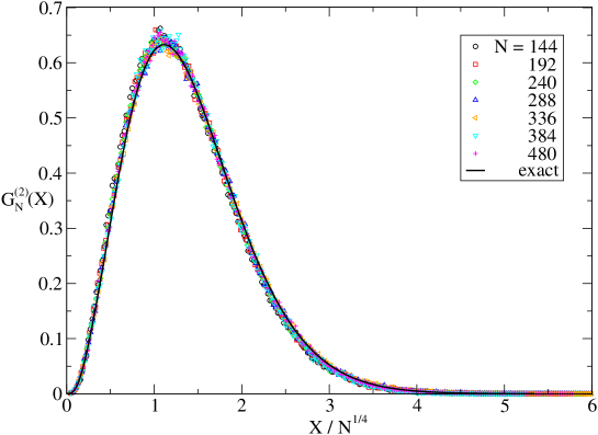
Figure 1: The two-point correlation function $G_{N}^{(2)}(X)$ for the Gaussian branched polymer model plotted against $X/N^{1/4}$.

We now turn to the branched polymers (8) derived from the matrix model (1). The two-point function for different system sizes is plotted against the scaling variable in figure 2. One can see small deviations from the scaling.

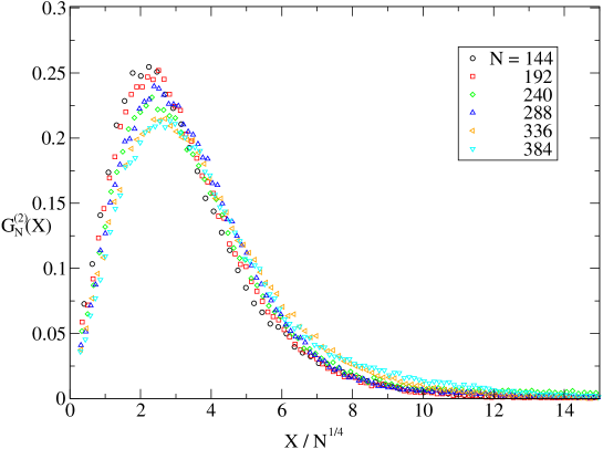
Figure 2: The two-point correlation function $G_{N}^{(2)}(X)$ for the branched polymer model with power-tail weights and a hard core $c=1$ plotted against $X/N^{1/4}$.

The reason for this behaviour is related to the presence of the power-law tail in the link length distribution $W(r)$ which leads to the divergence of the second moment of the distribution $\langle r^{2}\rangle=\int d^{4}r\,r^{2}W(r)\sim\int dr/r$ as already mentioned above. This means that fluctuations of the link lengths are infinite and that from time to time long links appear in the system. These links are reminiscent of the spiky configurations observed in the surface model [18]. Let us now try to understand algorithmical problems caused by the presence of such a fat-tailed distribution. The algorithm which we use is an example of dynamical Monte Carlo. It generates a Markov chain of configurations randomly walking in the configuration space. Any two consecutive configurations in the chain differ from each other only a little. In a single step the algorithm changes a link vector by a small value $\vec{r}\rightarrow\vec{r}+\vec{\delta}$ and accepts this change with the Metropolis probability. The sequence of changes can be viewed as a sort of random walk in the potential $\ln W(r)$. This potential is very flat and therefore if the algorithm once produces a long link it takes a long time to make it short again. Such a random walk algorithm introduces therefore large autocorrelation times. Moreover, a long excursion towards the tail of the distribution produces many long links, so after each long excursion a surplus of long links and a deficit of short ones occurs in the recorded history. This is an effect which makes the rescaled histograms in figure 2 not to coincide. The narrow tails of the histogram go far beyond the range in the figure. The tail behaviour of the two-point function is presented in the logarithmic scale in figure 3. It is compared with the tail behaviour of the original matrix model (1). The two-point correlation function inherits the power-law tail $drr^{-3}$ from the link length distribution $\sim drr^{3}W(r)$. As we can see in figure 3 in both cases the data behave as $\sim r^{-3}$.

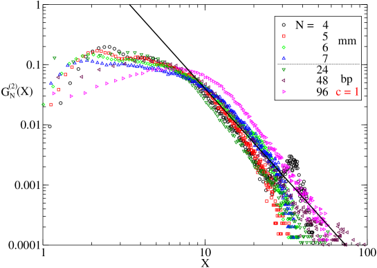
Figure 3: Comparison of the two-point function $G_{N}^{(2)}(X)$ of the branched polymer model with power-tail weights regularised by introducing a hard core $c=1$ and the IIB matrix model for different values of $N$. The solid black line illustrates the expected power-law behaviour: $\sim X^{-3}$.

The presence of the tails $\sim r^{-3}$ makes the determination of the linear extent of the system $R_{N}$ (14) difficult. The computation of $R_{N}$ amounts to the computation of the first moment of the two-point function. The autocorrelation time for the algorithm is large and grows with $N$. On the other hand one expects using the central limit theorem that the tail $r^{-3}$ belongs to the Gaussian universality class, what means that the probability of entering the tail part of the distribution decreases with the number of degrees of freedom, in our case with $N$. One therefore expects that in the limit $N\rightarrow\infty$ the quantity $R_{N}$ should depend on the bulk of the distribution and not on the tail which becomes marginal in this limit, and thus that the broadening of the statistical error coming from the large autocorrelation time should be finite for $R_{N}$ for large system sizes. One can use standard methods to estimate the error bars of $R_{N}$. If we do so we obtain the data presented in figure 4 illustrating the dependence of the linear extent $R_{N}$ on the system size.

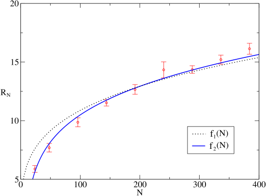
Figure 4: Comparison of the average gyration radius $R_{N}$ for the branched polymer model with a hard core $c=1$ plotted against the number of vertices $N$. The continuous lines represent the functions: $f_{1}(N)=3.44\cdot N^{1/4}$ and $f_{2}(N)=3.56\cdot N^{1/4}(1-6.8N^{-1})$.

The data presented in figure 4 can be fitted with the scaling formula $f_{1}(N)=a_{1}\cdot N^{1/4}$. If we apply this formula to find the best fit for the range $N>48$ we obtain $a_{1}=3.44(5)$ with the fit quality: $\chi^{2}_{dof}=2.9$. If we include finite size corrections $f_{2}(N)=a_{2}\cdot N^{1/4}(1+b_{2}N^{-1})$, then the best fit is for $a_{2}=3.56(4)$ and $b_{2}=-6.8(9)$ and has the quality $\chi^{2}_{dof}=1.1$. The fit quality improves in comparison with the previous one as can also be seen with the bare eye. The finite size corrections which control deviations from the pure scaling can be attributed to the power-law tails which now and then cause the appearance of a long link on the branched polymer and to the hard core repulsion which also effectively makes the polymer look more elongated. The repulsion disfavors crumpled trees. In principle one could expect the fractal dimension of branched polymers to lower. The magnitude of the finite size corrections in $f_{2}(N)$ is for $b_{2}=-6.8$ of order a few percent for $N$ is of order a few hundred. One can thus believe that the results are consistent with the fractal dimension $D_{f}=4$. To thoroughly check this hypothesis one would though have to study much larger systems.

5 Polyakov-line operator in the branched polymer model

In this section we will discuss measurements of the Polyakov-line operator. As it stands in equation (3) it has real and imaginary parts. The imaginary part however gives zero on average due to the reflection symmetry: the partition function of the branched polymer model is invariant with respect to simultanous reflections $\vec{x}_{i}\rightarrow-\vec{x}_{i}$ of all vertex positions and therefore the average value of the Polyakov-line operator over the ensemble of branched polymers fulfills the condition:

$$\left\langle P_{bp,k}[x]\right\rangle=\left\langle P_{bp,k}[-x]\right\rangle.$$ (15)

Thus it is sufficient to measure only the real part of the operator. We shall denote it by $P_{k}$. The momentum $\vec{k}$ plays the role of an external parameter. Since the branched polymer system is isotropic one can choose $\vec{k}$ to lie on one of the axes of the coordinate system in which components of the fields $\vec{x}_{i}$ are expressed. In practice, while doing numerical simulations one can calculate projections on the four independent components $\mu=1\ldots 4$ and average over them to improve statistics. This procedure eventually leads to the following operator

$${P}_{k}[x] = P^{(1)}_{k}[x]+P^{(2)}_{k}[x]+P^{(3)}_{k}[x]$$ (16)

where

$$P^{(1)}_{k}[x] = \frac{1}{4N}\sum_{\mu=1}^{4}\sum_{a}\cos(kx^{\mu}_{a})\ ,$$

$$P^{(2)}_{k}[x] = \frac{-k}{4N}\sum_{\mu=1}^{4}\sum_{a<b}\frac{\sin(kx_{a}^{\mu})-\sin(kx_{b}^{\mu})}{(x_{a}^{\mu}-x_{b}^{\mu})|x_{a}-x_{b}|^{2}}\ ,$$

$$P^{(2)}_{k}[x] = \frac{-k}{4N}\sum_{\mu=1}^{4}\sum_{\langle ab\rangle\in T}\frac{\sin(kx_{a}^{\mu})-\sin(kx_{b}^{\mu})}{(x_{a}^{\mu}-x_{b}^{\mu})|x_{a}-x_{b}|^{2}}\cdot\frac{2|x_{a}-x_{b}|^{2}-\left(x_{a}^{\mu}-x_{b}^{\mu}\right)^{2}}{3|x_{a}-x_{b}|^{2}}\ .$$

In the last equations $k$ stands for the length of the vector $\vec{k}$, which is independent of the space-time direction $\mu$. In particular $kx_{\mu}$ is a product of the length of the vector $\vec{k}$ and the $\mu$-th component of $\vec{x}$.

The length scale in the branched polymer model is set by the size of the core $c$. It is the only scale parameter in the model. The model is invariant under a simultaneous rescaling $c\rightarrow\lambda c$ and $\vec{x}_{i}\rightarrow\lambda\vec{x}_{i}$. One can use this invariance to rescale the core size to $c=1$. The average of an operator $O[x]$ over the ensemble of branched polymers with a hard core of size $c$ can be expressed as the average of this operator for the rescaled argument $O[cx]$ over the system with a core $c=1$:

$$\langle O[x]\rangle_{c}=\langle O[cx]\rangle_{c=1}\ .$$ (17)

In particular for an operator which is a homogeneous function of order $\Delta$: $O[\lambda x]=\lambda^{\Delta}O[x]$ we have

$$\langle O[x]\rangle_{c}=c^{\Delta}\langle O[x]\rangle_{c=1}\ .$$ (18)

The momentum $k$ of the Polyakov-line operator introduces an additional scale which has to be measured relatively to $c^{-1}$. If one rescales $\vec{x}\rightarrow\lambda\vec{x}$ one should simultaneously rescale $k\rightarrow k/\lambda$ to keep the combination $\vec{k}\vec{x}$ constant. We can now relate the value of the Polyakov-line in the system with a hard core $c$ to its value in the system with $c=1$:

$$\left\langle P^{(1)}_{k}[x]\right\rangle_{c}=\left\langle P^{(1)}_{ck}[x]\right\rangle_{c=1}\ ,\quad\left\langle P^{(2,3)}_{k}[x]\right\rangle_{c}=c^{-4}\left\langle P^{(2,3)}_{ck}[x]\right\rangle_{c=1}\ .$$ (19)

The amplitudes of the second $P^{(2)}_{k}[x]$ and the third term $P^{(3)}_{k}[x]$ scale as $c^{-4}$ with the core size while the amplitude of the first term $P^{(1)}_{k}[x]$ stays constant. Using this observation we can reconstruct the behaviour of the average of the Polyakov-line operator $\langle P_{k}\rangle_{c}$ in the system with an arbitrary $c$ from measurements of $\langle P^{(1)}_{k}\rangle$, $\langle P^{(2)}_{k}\rangle$ and $\langle P^{(3)}_{k}\rangle$ for $c=1$. We will follow this strategy. In figure 5 we present the dependence of the three contributions for $c=1$ on the momentum $k$, obtained by numerical Monte Carlo measurements.

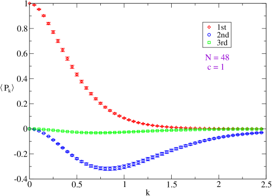
Figure 5: The three terms $\langle P^{(1)}_{k}\rangle_{c=1}$, $\langle P^{(2)}_{k}\rangle_{c=1}$ and $\langle P^{(3)}_{k}\rangle_{c=1}$ contributing to the average Polyakov-line operator in the one-loop approximation (16) in the system with hard core size $c=1$.

Since the second and the third terms are negative, the Polyakov-line operator being a linear combination of the three terms (16) may assume negative values for some range of $k$ depending on the value of $c$ (19). Such a behaviour is also observed in the matrix model for small $N$ as we can see in figure 6. In the matrix model the effect however disappears when $N$ increases and is practically absent already for $N$ of order ten. The curve for $N=2$ in figure 6 was obtained analytically as a Fourier transform of the eigenvalue distribution whose form is known for $SU(2)$ [23].

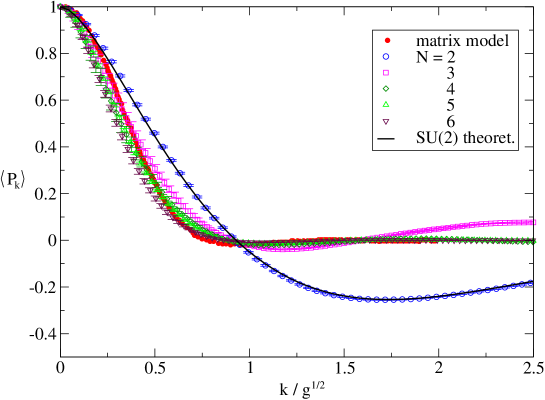
Figure 6: Comparing the Polyakov one-point correlation functions $\langle P_{k}\rangle$ of the IIB matrix model for $N=2,\,3,\,4,\,5,\ 6$.

Now the issue is to test up to what degree the model of branched polymers can reproduce the full matrix model. The model of branched polymers was constructed as an effective model for the large-distance behaviour of the original model. So we are now looking for the optimal value of the parameter $c$, which is a free parameter of the effective model, to reproduce the behaviour of the matrix model on large distances which correspond to small values of $k$ in the Polyakov-line operator. For the comparison we will use the matrix model results presented in [17]. They correspond to $N=16,\,24,\,32$ and $48$. The coupling constant $g$ of the matrix model is chosen to be $g=\sqrt{48/N}$ and the results are expressed in physical units $k_{\mbox{\tiny{phys}}}=k/\sqrt{g}$ [17]. After rescaling to physical units the data of the matrix model for different $N$ collapse to one curve. This curve goes as $1-\alpha k^{2}+\dots$ for small $k$. We found that for $c=0.75$ also the branched polymer results follow this curve in the region of small momenta. The results are presented in figure 7.

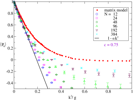
Figure 7: Comparing the $1-\alpha k^{2}+\dots$ behaviour of the Polyakov-line operator $\langle P_{k}\rangle$ of a branched polymer with $c=0.75$ for different sizes of $N$ and the IIB matrix model results.

Indeed for small $k$ the data points for different $N$ follow the same line $1-\alpha k^{2}$. The slope parameter $\alpha$ is thus universal. For larger $k^{2}$ the results depart from the universal line in a non-universal manner which depends on $N$. There are two reasons for that. First of all the effective model by construction is only supposed to describe the large-distance (small $k$) behaviour. For larger $k$ the effective model depends on the details of the regularization and is not any more universal. Secondly the Polyakov-line operator (3) contains only one-loop corrections. Higher loop corrections, which have been neglected in (3) would introduce terms of order $O(k^{4})$. Let us stress again, what is most important in figure 7 is that the leading $k^{2}$ behaviour is universal and identical with that of the original matrix model.

6 Summary

We have shown that the branched polymer model very well describes all essential features of the reduced supersymmetric Yang-Mills integrals in four dimensions at large distances: the power-law tail behaviour of the two-point function, the four dimensional scaling of the gyration radius and the universal small momentum behaviour of the Polyakov-line operator. The branched polymer model can thus be useful in studies of the low momentum content of supersymmetric QCD [22].

What remains to be checked is whether the one-loop approximation works equally well for the ten dimensional matrix model where branched polymers are replaced by somewhat more complex graphs in the effective model. These graphs have branched polymer backbones and one believes that they preserve the four dimensional fractal structure. Additional links which appear on the graphs introduce some rigidity constraints which therefore may make the fractal dimension to become the canonical dimension of the underlying geometry. This would explain the existence of a dynamical spontaneous symmetry breaking of the original ten dimensional Lorentz symmetry. There are some indications that such a scenario indeed takes place [9, 10, 11, 12, 13, 24, 25].

Acknowledgments

This work was partially supported by the Deutsche Forschungsgemeinschaft under the project FOR 339/2-1, the Polish State Committee for Scientific Research (KBN) grant 2P03B-08225 (2003-2006) and by EU IST Center of Excellence “COPIRA”.

References

- [1] N. Ishibashi, H. Kawai, Y. Kitazawa and A. Tsuchiya, Nucl. Phys. B498 (1997) 467.
- [2] M. Fukuma, H. Kawai, Y. Kitazawa and A. Tsuchiya, Nucl. Phys. B510 (1998) 158.
- [3] H. Aoki, S. Iso, H. Kawai, Y. Kitazawa, A. Tsuchiya and T. Tada, Prog. Theor. Phys. Suppl. 134 (1999) 47.
- [4] H. Aoki, S. Iso, H. Kawai, Y. Kitazawa and T. Tada, Prog. Theor. Phys. 99 (1998) 713.
- [5] W. Krauth, H. Nicolai and M. Staudacher, Phys. Lett. B431 (1998) 31.
- [6] J. Ambjørn, B. Durhuus and T. Jonsson, Quantum Geometry, Cambridge University Press, 1997.
- [7] H. Aoki, S. Iso, H. Kawai and Y. Kitazawa Phys.Rev. E62 (2000) 6260-6269.
- [8] Z. Burda, J. Erdmann, B. Petersson and M. Wattenberg, Phys. Rev. E67 (2003) 026105.
- [9] J. Nishimura and F. Sugino, JHEP 05 (2002) 001.
- [10] H. Kawai, S. Kawamoto, T. Kuroki, T. Matsuo and S. Shinohara, Nucl. Phys. B647 (2002) 153.
- [11] G. Vernizzi and J.F. Wheater, Phys. Rev. D66 (2002) 085024.
- [12] H. Kawai, S. Kawamoto, T. Kuroki and S. Shinohara, Prog. Theor. Phys. 109 (2003) 115.
- [13] K. N. Anagnostopoulos and J. Nishimura, Phys. Rev. D66 (2002) 106008.
- [14] S. Oda and F. Sugino, JHEP 0103 (2001) 026.
- [15] F. Sugino, JHEP 0107 (2001) 014.
- [16] J. Ambjørn, K. N. Anagnostopoulos, W. Bietenholz, T. Hotta and J. Nishimura, JHEP 07 (2000) 011.
- [17] J. Ambjørn, K. N. Anagnostopoulos, W. Bietenholz, T. Hotta and J. Nishimura, JHEP 07 (2000) 013.
- [18] P. Bialas, Z. Burda, B. Petersson and J. Tabaczek, Nucl. Phys. B592 (2001) 391.
- [19] Z. Burda, B. Petersson and J. Tabaczek, Nucl. Phys. B602 (2001) 399.
- [20] Z. Burda, B. Petersson and M. Wattenberg, Acta Phys. Pol. B34 (2003), 4765.
- [21] T. Eguchi and H. Kawai, Phys.Rev.Lett. 48 (1982) 1063.
- [22] D. J. Gross and Y. Kitazawa, Nucl.Phys. B206 (1982) 440.
- [23] W. Krauth, J. Plefka and M. Staudacher, Class. Quant. Grav. 17 (2000) 1171.
- [24] J. Ambjørn, K. N. Anagnostopoulos, W. Bietenholz, F. Hofheinz and J. Nishimura, Phys. Rev. D65 (2002) 086001.
- [25] J. Nishimura, T. Okubo and F. Sugino, hep-th/0412194.