A Higgs Mechanism for Gravity

Abstract

In this paper we elaborate on the idea of an emergent spacetime which arises due to the dynamical breaking of diffeomorphism invariance in the early universe. In preparation for an explicit symmetry breaking scenario, we consider nonlinear realizations of the group of analytical diffeomorphisms which provide a unified description of spacetime structures. We find that gravitational fields, such as the affine connection, metric and coordinates, can all be interpreted as Goldstone fields of the diffeomorphism group. We then construct a Higgs mechanism for gravity in which an affine spacetime evolves into a Riemannian one by the condensation of a metric. The symmetry breaking potential is identical to that of hybrid inflation but with the non-inflaton scalar extended to a symmetric second rank tensor. This tensor is required for the realization of the metric as a Higgs field. We finally comment on the role of Goldstone coordinates as a dynamical fluid of reference.

I Introduction

Recent discoveries in cosmology have shown that general relativity is most likely incomplete. In particular the high degree of homogeneity and isotropy of the universe can only be understood by supplementing Einstein’s theory with an inflationary scenario. Also the accelerating expansion of the universe by dark energy might hint to a further modification of general relativity.

Most of these additions to general relativity introduce new fields in a quite ad hoc way. For instance, inflationary models typically postulate one or two scalar fields which drive a rapid expansion of the early universe. Even in general relativity the metric is not derived from any underlying symmetry principle. An exception are gauge theories of gravity in which the existence of a connection is justified by the gauging. Also in ghost condensation Nima the dynamical field appears as the Goldstone boson of a spontaneously broken time diffeomorphism symmetry. However, in many other cases the group theoretical origin of the gravitational fields remains unclear.

In this paper we show that the existence of most of these fields can be understood in terms of Goldstone bosons which arise in a rapid symmetry breaking phase shortly after the Big Bang.

We assume that at the beginning of the universe all spacetime structures were absent and consider the universe as a Hilbert space ${\cal H}$ accommodating spinor and tensor representations of the analytic diffeomorphism group $\overline{\textit{Diff}}\,(n,\mathbb{R})$. Unlike in general relativity spinors and tensors are representations of the same covering group $\overline{\textit{Diff}}\,(n,\mathbb{R})$ whose existence has been shown in Neeman . Since spinor representations of $\overline{\textit{Diff}}\,(n,\mathbb{R})$ are necessarily infinite-dimensional Neeman , matter would look quite exotic at this stage. Here we are however not so much interested in the structure of these representations. For our purposes, it is enough to suppose that they do exist.

We further assume that in a series of spontaneous symmetry breakings, the transformation group $H$ of states in the Hilbert space collapsed down to the Lorentz group. We suggest that the symmetry breaking sequence is given by the group inclusion

$$\overline{\textit{Diff}}\,(n,\mathbb{R})\stackrel{{\scriptstyle TR}}{{\supset}}\overline{\textit{Diff}}_{0}(n,\mathbb{R})\stackrel{{\scriptstyle NL}}{{\supset}}\overline{GL}(n,\mathbb{R})\stackrel{{\scriptstyle SD}}{{\supset}}\overline{SO}(1,n-1)$$

where $\overline{\textit{Diff}}_{0}(n,\mathbb{R})$ is the homogeneous part of the diffeomorphism group, $\overline{GL}(n,\mathbb{R})$ the general linear group and $\overline{SO}(1,n-1)$ the Lorentz group. This corresponds to the breaking of translations (TR), nonlinear transformations (NL), dilations and shear transformations (SD), respectively.

The existence of such a symmetry breaking scenario appears more convincing if it is considered from bottom up. At low temperatures the vacuum is invariant under local Lorentz transformations and matter is represented by Lorentz spinors. It is conceivable that at higher temperatures matter transforms under a larger spacetime group. The most prominent example is scale invariance which is believed to be restored at high energies. Here matter is described by spinors of the conformal group which contains the Lorentz group as a subgroup. It is not implausible that further symmetries of the diffeomorphism group and in the end all of them are restored at very high temperatures.

So far we focused exclusively on the breaking of the transformation group $H$ of states in the Hilbert space. After a series of phase transitions, matter is again represented by spinors of the Lorentz group rather than the diffeomorphism group. The appealing aspect of this view of matter is that gravitational fields emerge naturally as Goldstone bosons of the symmetry breaking (quasi as a by-product). In each phase of the breaking we loose degrees of freedom in the matter sector, i.e. states in the Hilbert space, but gain new geometrical objects in terms of Goldstone fields. Spacetime appears as an emergent product of this process.

A convenient concept to determine these Goldstone bosons is given by the nonlinear realization approach Colea ; Coleb ; Salaa ; Salab . This technique provides the transformation behavior of fields $\xi$ of a coset space $G/H$ which is associated with the spontaneous breaking of a symmetry group $G$ down to a stabilizing subgroup $H$. Nonlinear realizations of spacetime groups have been studied in a number of papers Isha ; Bori ; Pash ; Tseytlin ; Tres ; Puli ; Lope ; Ogie74 ; Lord1 ; Lord2 ; Ivanov:1981wn . As in Bori ; Pash we consider nonlinear realizations of the diffeomorphism group, i.e. we choose $G=\textit{Diff}\,(n,\mathbb{R})$ and $H$ to be one of the groups in the above sequence. It turns out that in this way the relevant gravitational fields, such as coordinates, affine connection and metric, are all of the same nature: They can be identified with Goldstone bosons or coset fields of the diffeomorphism group.

Let us have a brief look at the nonlinear realizations in detail. The first nonlinear realization with $H_{0}=\textit{Diff}_{0}(n,\mathbb{R})$ corresponds to the breaking of translational invariance and shows the existence of dynamical coordinates in terms of Goldstone fields. Subsequently, we realize $\textit{Diff}\,(n,\mathbb{R})$ with $H_{1}=GL(n,\mathbb{R})$ as stability group. The corresponding coset fields transform as a holonomic affine connection and can be used for an affine theory of gravity. Finally, we realize $\textit{Diff}\,(n,\mathbb{R})$ with the Lorentz group $H_{2}=SO(1,n-1)$ as stability group corresponding to the additional breaking of dilations and shear transformations. The corresponding coset parameters can be interpreted as tetrads which lead to the definition of a metric. This has already been found by Borisov and Ogievetsky Bori who studied a simultaneous realization of the affine and the conformal group with the Lorentz group as stability group.

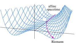
Figure 1: The potential $V(\varphi_{ij},\phi)$. The metric is conformally flat for $\phi>\phi_{c}$, tachyonic for $\phi<\phi_{c}$ and becomes massless at the minimum of the potential at $\phi=0$, $|\varphi_{ij}|=\pm M$.

$V$

$\phi$

$|\varphi_{ij}|$

${M}$

$\mathbf{\phi_{c}}$

Though nonlinear realizations of spacetime groups have been studied for quite some time, with a few exceptions West ; Kirsch ; Sija88 ; Leclerc:2005qc ; Percacci:1990wy ; Percacci ; Wilczek:1998ea , there have not as yet been developed any Higgs models for the dynamical breaking of these groups. In this paper we construct such a gravitational Higgs mechanism by introducing the metric as a Higgs field into an affine spacetime. This effectively corresponds to a metric-affine theory of gravity MAG in which $GL(4,\mathbb{R})$ breaks down to $SO(1,3)$ in the tangent space of the spacetime manifold.

The Higgs sector is constructed as follows. In analogy to the isospinor scalar $\Phi=(\phi^{+},\phi^{0})$ of electroweak symmetry breaking, the breaking is induced by a (real) scalar field $\phi$ and a symmetric tensor $\varphi_{ij}$ which has ten independent components. Under the Lorentz group the tensor $\varphi_{ij}$ decomposes into its trace $\sigma$ and a traceless tensor $\hat{\varphi}_{ij}$ according to ${\bf 10\rightarrow 1+9}$. The singlet $\sigma$ turns out to be a massive gravitational Higgs field, whereas the fields $\hat{\varphi}_{ij}$ and $\phi$ are the ten Goldstone fields associated with the coset $GL(4,\mathbb{R})/SO(1,3)$. As shown by the nonlinear realization approach, these fields define the metric

$$g_{ij}=e_{i}{}^{\alpha}e_{j}{}^{\beta}\eta_{\alpha\beta}\,,\quad e_{i}{}^{\alpha}\equiv\phi\exp\left(i\hat{\varphi}_{jk}\hat{T}^{jk}\right){}_{i}{}^{\alpha}\,,$$ (1)

where $\hat{T}^{ij}$ are the shear generators and $\phi$ parameterizes dilations. In Tab. 1 we compare the Higgs sector of the electroweak symmetry breaking with that in gravity.

symmetry breaking	electroweak	gravity
symmetry	$SU(2)\times U(1)_{Y}$	$GL(4,\mathbb{R})$
stabilizer	$U(1)_{EM}$	$SO(1,3)$
Higgs field $\Phi$	$(\phi^{0},\phi^{+})$	$(\varphi_{ij},\phi)$
# components of $\Phi$	$4$	$10+1$
# Goldstone bosons	$3$	$10$
# Higgs particles	$1$	$1$
massive bosons	$W^{\pm},Z$	$Q_{ijk}$

Table 1: A comparison of the electroweak symmetry breaking and the Higgs mechanism in gravity. $Q_{ijk}\equiv\nabla_{k}g_{ij}$ is the nonmetricity tensor.

The symmetry breaking potential $V(\varphi_{ij},\phi)$ in our model is similar to that of hybrid inflation hybrid with $\phi$ the inflaton and $\varphi_{ij}$ replacing the non-inflaton scalar. As shown in Fig. 1, the field $\phi$ rolls down the channel at $\varphi_{ij}=0$ until it reaches a critical value $\phi_{c}$ at which point $\varphi_{ij}=0$ becomes unstable and the field rolls down to the minimum of the potential at $\phi=0$ and $|\varphi_{ij}|=\pm M$. In other words, the breaking of dilations triggers the spontaneous breaking of shear symmetry and induces the condensation of the metric $g_{ij}$.

During the condensation the affine connection absorbs the metric. Some degrees of freedom of the connection known as nonmetricity $Q_{ijk}$ acquire a mass as a consequence of “eating” the Goldstone metric. This is the analog of the absorption of Goldstone bosons by the gauge bosons of $SU(2)\times U(1)_{Y}$ which become massive $W^{\pm}$ and $Z$ bosons. The mass of the nonmetricity is however of order of the Planck scale such that nonmetricity decouples at low energies. If we also neglect torsion, then the affine connection turns into the Christoffel connection and we recover an effective Riemannian spacetime at the minimum of the potential, see Fig. 1.

The paper is organized as follows. In section II we review several aspects of the diffeomorphism algebra and sketch the nonlinear realization technique in order to fix the notation. We also discuss principles of gravity and their relation to nonlinear realizations of the diffeomorphism group. In section III we show that coordinates, metric and connection can all be identified as Goldstone bosons of the diffeomorphism group. In section IV we construct the Higgs model for the condensation of the metric in an affine spacetime. We conclude in section V with some final remarks and some open questions. Many detailed computations of the nonlinear realizations can be found in the appendix.

II Principles of gravity and nonlinear realizations of the diffeomorphism group

In this section we briefly review the algebra of analytic diffeomorphisms and the nonlinear realization technique. We also discuss the relation between principles of gravity and nonlinear realizations of the diffeomorphism group. We suggest that the two groups involved in these nonlinear realizations are unambiguously fixed by the principle of general covariance and an appropriate equivalence principle.

II.1 Principles of theories of gravity

Classical theories of gravity are explicitly or implicitly based on two invariance principles. The first one is the principle of general covariance. What is actually meant by general covariance has often been the subject of discussion in the literature, see e.g. Ref. 9910079 . General covariance does not just mean invariance under general coordinate transformations, since every theory can be made invariant under (passive) diffeomorphisms as has already been pointed out by Kretschmann Kret . It is not obvious how the group of diffeomorphisms selects the metric or the affine connection as the dynamical field in a theory of gravity. We will show below that nonlinear realizations of the diffeomorphism group give these fields a group theoretical foundation.

In addition to the principle of general covariance, theories of gravity also require a hypothesis about the geometry of spacetime. The latter is mostly disguised in the formulation of an equivalence principle (EP). We know at least three classical EP’s, see e.g. Laem : the weak (WEP), the strong (SEP) and Einstein’s equivalence principle (EEP). Each EP determines a particular geometry: While the WEP postulates a quite general geometry (Finslerian e.g.), the SEP restricts spacetime to be affine. Finally, EEP assumes local Lorentz invariance leading to a Riemannian geometry.

From the perspective of the nonlinear realization technique, it is not a coincidence that theories of gravity are based on exactly two postulates. As we will review in Sec. II.3, there are two groups, $G$ and $H$, involved in a nonlinear realization: The group $G$ is represented nonlinearly over one of its subgroups $H$. It is quite plausible that these groups are fixed by the principle of general covariance and an appropriate equivalence principle. The former fixes $G$ to be the diffeomorphism group, $G=\textit{Diff}\,(n,\mathbb{R})$, while the later fixes $H$ to be either the general linear group $H_{1}=GL(n,\mathbb{R})$ (in case of the SEP) or the Lorentz group $H_{2}=SO(1,~{}n-1)$ (in case of the EEP). We will see in Sec. III that such nonlinear realizations lead to an affine or a Riemannian spacetime, respectively.

II.2 The group of analytic diffeomorphisms

In the following we briefly discuss the algebra of analytic diffeomorphisms. Representations of the group Diff$(n,\mathbb{R})$ can be defined in an appropriate Hilbert space of analytic functions $\Psi_{A}(x^{i})$. We make the assumption that the manifold, on which $\Psi_{A}$ is defined, locally allows for a Taylor expansion. The generators can be expressed in terms of coordinates $x^{i}$ as $(m=-1,...,\infty$; $i,j_{a}=0,...,n-1$; $a=1,...,m+1$) Sija83 ; Bori2

$$F^{m}_{i}{}^{j_{1}...j_{m+1}}\Psi_{A}=$$

$$\hskip 14.22636pt\underbrace{ix^{j_{1}}...x^{j_{m+1}}\frac{\partial}{\partial x^{i}}\Psi_{A}}_{\rm orbital}+\underbrace{i(\hat{F}_{i}{}^{j_{1}...j_{m+1}})_{A}{}^{B}\Psi_{B}\frac{}{}}_{\rm intrinsic}\,$$ (2)

with the intrinsic part $(m\geq 0)$

$$\hat{F}_{i}{}^{j_{1}...j_{m}}=\partial_{k}(x^{j_{1}}...x^{j_{m}})\hat{L}_{i}{}^{k},$$ (3)

where $\hat{L}_{i}{}^{k}$ are representations of $\overline{GL}(n,\mathbb{R})$. The generators have one lower index and are symmetric in the $m+1$ upper indices. The lowest generators ($m=-1,0$) are the translation operators $P_{i}\equiv F_{i}^{-1}$ and the operators of the linear group $L_{i}{}^{j}\equiv F^{0}_{i}{}^{j}$. Generators $F^{m}$ with $m\geq 1$ generate nonlinear transformations.

The generators of Diff$(n,\mathbb{R})$ satisfy the commutation relations

$$[F^{n}_{k}{}^{i_{1}...i_{n+1}},F^{m}_{l}{}^{j_{1}...j_{m+1}}]=$$

$$\hskip 14.22636pt=i\sum\limits_{a=1}^{m+1}\delta^{j_{a}}_{k}F^{m+n}_{l}{}^{i_{1}...i_{n+1}j_{1}...\hat{j}_{a}...j_{m+1}}$$

$$\hskip 14.22636pt-i\sum\limits_{a=1}^{n+1}\delta^{i_{a}}_{l}F^{m+n}_{k}{}^{i_{1}...\hat{i}_{a}...i_{n+1}j_{1}...j_{m+1}},$$ (4)

where the indices with a hat are omitted. Two important subalgebras are the algebras of the linear group $GL(n,\mathbb{R})$ and the Lorentz group $SO(1,n-1)$ with commutation relations

$$[L_{i}{}^{j},L_{k}{}^{l}]=i\delta_{i}^{l}L_{k}{}^{j}-i\delta_{k}^{j}L_{i}{}^{l}\,$$ (5)

and

$$[M_{ij},M_{kl}]=i\eta_{il}M_{kj}-i\eta_{jl}M_{ki}-i\eta_{kj}M_{il}+i\eta_{ki}M_{jl},$$ (6)

where $M_{ij}\equiv L_{[i}{}^{k}\eta_{j]k}$ are the Lorentz generators.

II.3 Nonlinear realizations

Let us briefly summarize the nonlinear realization technique Colea ; Coleb ; Salaa ; Salab . In order to fix the notation, we only list some important formulas which we use throughout this paper.

Nonlinear realizations are based on the notion of a fiber bundle. Let $H$ be a closed not invariant subgroup of a Lie group $G$. Then $G/H=\{gH,g\in G\}$ is a homogeneous space not a group and $G$ can be decomposed as

$$G=\{H\cup g_{1}H\cup g_{2}H\cup...\},$$ (7)

where $g_{1}\notin H,g_{2}\notin\{H,g_{1}H\}$, etc. This means that $G$ can be written as a union of spaces $\{g_{i}H\}$, all diffeomorphic to $H$ and parameterized by the coset space $G/H$. So the group $G$ can be regarded as a principal fiber bundle with structure group $H$, base space $G/H$, and projection $\sigma^{-1}:G\rightarrow G/H$.

Assume a group $G$ shall be represented nonlinearly over one of its subgroups $H$. Following Colea ; Coleb ; Salaa ; Salab , the fundamental nonlinear transformation law for elements $\sigma$ of $G/H$ is given by

$$g\sigma(\xi)=\sigma(\xi^{\prime})h(\xi,g)\,.$$ (8)

An element $\sigma(\xi)$ is transformed into another element $\sigma(\xi^{\prime})$ by multiplying it with $g\in G$ from the left and with $h^{-1}\in H$ from the right.

The standard form of an element $\sigma\in G/H$ is given by

$$\sigma(\xi)\equiv e^{i\xi^{i}A_{i}}\,,$$ (9)

where $A_{i}$ are the generators of the coset space $G/H$ and $\xi^{i}$ the corresponding coset parameters. Eq. (8) defines implicitly the nonlinear transformation $\xi\rightarrow\xi^{\prime}$, i.e. the transformation behavior $\delta\xi$ of the coset parameters $\xi$.

In the nonlinear realization of symmetry groups the total connection is given by the Maurer-Cartan 1-form

$$\Gamma\equiv\sigma^{-1}d\sigma\,.$$ (10)

By differentiation of Eq. (8) with respect to the coset fields $\xi$, we obtain $gd\sigma=d\sigma^{\prime}h+\sigma^{\prime}dh$ and from this the nonlinear transformation law

$$\Gamma^{\prime}=h\Gamma h^{-1}+hdh^{-1}\,.$$ (11)

The total connection $\Gamma$ can be divided into pieces $\Gamma_{\rm H}$ and $\Gamma_{\rm G/H}$ defined on the subgroup $H$ and the space $G/H$, respectively. The transformation law (11) then shows that $\Gamma_{\rm H}$ transforms inhomogeneously, whereas $\Gamma_{\rm G/H}$ transforms as a tensor:

$$\Gamma^{\prime}_{\rm H} =h\Gamma_{\rm H}h^{-1}+hdh^{-1}\,,$$

$$\Gamma^{\prime}_{\rm G/H} =h\Gamma_{\rm G/H}h^{-1}\,.$$ (12)

In other words, only $\Gamma_{\rm H}$ is a true connection which can be used for the definition of a covariant differential

$$D\psi\equiv(d+\Gamma_{\rm H})\psi\,$$ (13)

acting on representations $\psi$ of $H$.

At first sight one might think that the curvature $R\equiv d\Gamma+\Gamma\wedge\Gamma$ vanishes identically since $\Gamma=\sigma^{-1}d\sigma$. However, any Cartan form with a homogeneous transformation law can be put equal to zero Ivan . This is an invariant condition and does not affect physics. Because of the homogeneous transformation behavior of $\Gamma_{\rm G/H}$, only the curvature $R_{\rm H}\equiv d\Gamma_{\rm H}+\Gamma_{\rm H}\wedge\Gamma_{\rm H}$ is physically relevant.

III Nonlinear realizations of the diffeomorphism group

In this section we nonlinearly realize the group of diffeomorphisms $G=\textit{Diff}\,\mbox{$(n,\mathbb{R})$}$ over the homogeneous part of the diffeomorphism group $H_{0}=\textit{Diff}_{0}\mbox{$(n,\mathbb{R})$}$, the general linear group $H_{1}=GL(n,\mathbb{R})$ and the Lorentz group $H_{2}=SO(1,n-1)$. We show that the parameters of the corresponding coset spaces $G/H$ ($H\in\{H_{1},H_{2}\}$) can be identified with the geometrical objects of an affine and a Riemannian spacetime, respectively. In particular, we find that the parameters $\xi^{i}$, $h^{ij}$, and $\omega^{i}{}_{jk}$ associated to the generators $P_{i}\equiv F^{-1}_{i}$ (translations), $T_{ij}\equiv F^{0}_{(ij)}$ (shear transformations), and $F^{1}_{i}{}^{jk}$ transform as coordinates, metric, and affine connection.

III.1 The origin of a manifold ($\mathbf{G}$-coordinates)

The basic component of spacetime is a differentiable manifold with a local coordinate system. In this section we reveal the group theoretical origin of coordinates by constructing the coset space $G/H_{0}$ with $G=\textit{Diff}\,(n,\mathbb{R})$ and $H_{0}=\textit{Diff}_{0}\,(n,\mathbb{R})$ its homogeneous subgroup. This corresponds to the breaking of translations $x^{i}\rightarrow x^{i}+a^{i}$ in the representation space of the diffeomorphism group.

For the construction of the coset $G/H_{0}$ it is convenient to write an element $g\in G$ as

$$g=e^{i\varepsilon^{i}P_{i}}e^{i\varepsilon^{i}{}_{j}L_{i}{}^{j}}e^{i\varepsilon^{i}{}_{jk}F^{1}_{i}{}^{jk}}u\,,$$ (14)

with $u$ parameterizing that part of the diffeomorphism group which is spanned by the generators $F^{n}$ $(n\geq 2)$. The coset space $G/H_{0}$ is just spanned by the translation generators $P_{i}$ and elements $\sigma\in G/H_{0}$ can be written as

$$\sigma=e^{i\xi^{i}P_{i}}\,,$$ (15)

where the fields $\xi^{i}$ are the corresponding coset parameters.

In general, the total nonlinear connection $\Gamma$ can be expanded in the generators of $\textit{Diff}\,(n,\mathbb{R})$ as

$$\Gamma\equiv\sigma^{-1}d\sigma=i\vartheta^{i}P_{i}+i\Gamma^{i}{}_{j}L_{i}{}^{j}+i\Gamma^{i}{}_{jk}F^{1}_{i}{}^{jk}+...\,,$$ (16)

i.e. $\Gamma$ can be divided into a translational $\vartheta^{i}$, a linear $\Gamma^{i}{}_{j}$ and a nonlinear part, where $\vartheta^{i}$, $\Gamma_{i}{}^{j}$, etc. are vector-, tensor-valued etc. 1-forms, respectively.

The coset parameters $\xi^{i}$ have three interesting properties. First, as shown in App. A.1, the transformation law (8) for the elements $\sigma$ determines the transformation behavior of $\xi^{i}$ under $\textit{Diff}\,(n,\mathbb{R})$,

$$\delta\xi^{i}=\varepsilon^{i}(\xi)\equiv\varepsilon^{i}+\varepsilon^{i}{}_{j}\xi^{j}+\varepsilon^{i}{}_{jk}\xi^{j}\xi^{k}+...\,.$$ (17)

This is the transformation behavior of coordinates leading to the interpretation of the base space $G/H_{0}$ as a differentiable manifold with coordinates $\xi^{i}$. Second, the translational piece of the total connection $\Gamma$ turns out to be the coordinate coframe $\vartheta^{i}\equiv d\xi^{i}$ as can be seen by computing Eq. (16). Consequently, the coordinates $\xi^{i}$ cannot be distinguished from ordinary coordinates. Third, as shown by the computation in App. A.1, the parameters of the diffeomorphism group are promoted to fields which become explicit functions of the coordinates $\xi^{i}$, i.e. $\epsilon^{i}\rightarrow\epsilon^{i}(\xi)$, $\epsilon^{i}{}_{j}\rightarrow\epsilon^{i}{}_{j}(\xi)$, etc. This will become important below when we interpret other parameters of the diffeomorphism group as geometrical fields.

The breaking of global translations $x^{i}\rightarrow x^{i}+a^{i}$ in the representation space $\cal H$ of $\textit{Diff}\,(n,\mathbb{R})$ is achieved by the selection of a preferred point or an origin in this space. This is shown in Fig. 2. In this way no further symmetries are broken. The origin arises naturally in nonlinear realizations of $\textit{Diff}\,(n,\mathbb{R})$ as the point at which the manifold ${\cal M}=G/H_{0}$ is attached (“soldered”) to ${\cal H}$. This reflects the fact that the representation space ${\cal H}$ has become the tangent space of the manifold $G/H_{0}$.

A comment about the difference of the coordinates $x^{i}$ and $\xi^{i}$ is in order. The coordinates $x^{i}$ are non-dynamical and are necessary for the definition of the representation (II.2) of Diff$(n,\mathbb{R})$. These coordinates should not be confused with the coordinates $\xi^{i}$. In contrast to $x^{i}$, the coordinates $\xi^{i}$ represent a dynamical field. The dynamical character of the coordinates $\xi^{i}$ follows from the nonlinear realization approach: Each coset field, which is not eliminated by the inverse Higgs effect Ivan , is a Goldstone field and as such a dynamical quantity.

In Sec. III.2 and III.3 we will identify both the metric and the affine connection with further parameters of the diffeomorphism group, i.e. both fields turn out to be Goldstone fields, too. Since metric and connection are generally considered as dynamical quantities, also the Goldstone coordinates $\xi^{i}$ should be regarded in this way.

In order to be a true Goldstone field, the G-coordinates $\xi^{i}$ must result from a broken symmetry. Indeed, global translations $x^{i}\rightarrow x^{i}+a^{i}$ are broken in the representation space $\cal H$ and the coset parameters $\xi^{i}$ are the corresponding Goldstone fields. At the same time the parameters $\xi^{i}$ form the base manifold $G/H_{0}$ which is interpreted as a spacetime manifold by the identification of the $\xi^{i}$ with coordinates. This leads to reparameterization or diffeomorphism invariance of the spacetime manifold, see Eq. (17). Due to the isomorphism of the diffeomorphism group with the group of local translations, ${\cal T}\approx\textit{Diff}\,(n,\mathbb{R})$, we gained local translational invariance on the (external) spacetime manifold $G/H_{0}$ at the expense of loosing global translational invariance in the (internal) representation space $\cal H$.

This implies that general covariance in the sense of diffeomorphism invariance on the spacetime manifold $G/H_{0}$ is not broken and energy-momentum is preserved. Diffeomorphism invariance is however broken in the representation space ${\cal H}$.

Figure 2: The breaking of translational invariance.

Because of their dynamical behavior, G-coordinates may be visualized as a “fluid” of reference pervading the universe. Considering G-coordinates as a continuum, we would interpret the dynamical field $\xi^{i}(x)$ as the comoving body frame, whereas the nondynamical coordinates $x^{i}$ would be the reference frame. Such a continuum mechanical view might remind some of the readers of the concept of an ether. However, “ether” is not an adequate name, since G-coordinates are not a medium consisting of matter fields. They form a pure gravitational field just like the metric.

It is clear that a dynamical view of coordinates opens up the possibility of constructing new cosmological models. For instance, ghost condensation Nima describes the field $\phi\equiv\xi^{0}$ as a non-diluting cosmological fluid which possibly drives the accelerating expansion of the universe. We come back to this issue in Sec. IV.3 in which we discuss some properties of condensation models for the G-coordinates.

III.2 The origin of an affine connection

The emergence of coordinates as coset parameters of Diff $(n,\mathbb{R})$ is not surprising, since the diffeomorphism group is the group of general coordinate transformations. It is however remarkable that other gravitational fields can also be identified with parameters of the diffeomorphism group. This will now be shown for the affine connection.

For this purpose let us consider the parameters $\omega^{i}{}_{jk}$ which together with the G-coordinates $\xi^{i}$ parameterize the coset $G/H_{1}$ with $H_{1}=GL(n,\mathbb{R})$. An element of $G/H_{1}$ is given by

$$\sigma=\tilde{\sigma}u=e^{i\xi^{i}P_{i}}e^{i\omega^{i}{}_{jk}F^{1}_{i}{}^{jk}}u$$ (18)

with $u$ as in Eq. (14). The transformation behavior of $\omega^{i}{}_{jk}$ is determined by introducing the infinitesimal group elements $g\in\textit{Diff}\,(n,\mathbb{R})$ and $h\in GL(n,\mathbb{R})$ together with $\sigma$ in the nonlinear transformation law (8). As shown in detail in App. A.2, this gives

$$\delta\omega^{i}{}_{jk}=\frac{\partial\varepsilon^{i}}{\partial\xi^{l}}\omega^{l}{}_{jk}-\frac{\partial\varepsilon^{l}}{\partial\xi^{j}}\omega^{i}{}_{lk}-\frac{\partial\varepsilon^{l}}{\partial\xi^{k}}\omega^{i}{}_{jl}+\frac{1}{2}\frac{\partial^{2}\varepsilon^{i}}{\partial\xi^{j}\partial\xi^{k}}\,,$$ (19)

which is the transformation behavior of an affine connection. Due to the symmetry in the contravariant indices of the generator $F^{1}_{i}{}^{jk}$, the coset parameters $\omega^{i}{}_{jk}$ are symmetric in the indices $j$ and $k$. The connection $\omega^{i}{}_{jk}$ has only 40 independent components instead of $64$ (for $n=4$).

Moreover, for the total nonlinear connection we find

$$\Gamma =\sigma^{-1}d\sigma=u^{-1}\tilde{\sigma}^{-1}d\tilde{\sigma}u+u^{-1}du=\tilde{\sigma}^{-1}d\tilde{\sigma}+O(F^{1})$$

$$=e^{-i\omega^{i}{}_{jk}F^{1}_{i}{}^{jk}}(id\xi^{l}P_{l})e^{i\omega^{i}{}_{jk}F^{1}_{i}{}^{jk}}+O(F^{1})$$

$$=id\xi^{i}P_{i}+\omega^{i}{}_{jk}d\xi^{l}[F^{1}_{i}{}^{jk},P_{l}]+O(F^{1})$$

$$=i\vartheta^{i}P_{i}+i{\Gamma^{i}{}_{j}}L_{i}{}^{j}+O(F^{1}),$$ (20)

with

$$\vartheta^{i}\equiv d\xi^{i},\quad{\Gamma^{i}{}_{j}}\equiv\Gamma^{i}{}_{jk}d\xi^{k}=-2\omega^{i}{}_{jk}d\xi^{k}\,.$$ (21)

The physical part of the total connection $\Gamma$, which acts on matter via the covariant derivative, is given by its linear part

$$\Gamma_{\rm H_{1}}\equiv i{\Gamma^{i}{}_{j}}L_{i}{}^{j}$$ (22)

whose components $\Gamma^{i}{}_{jk}=-2\omega^{i}{}_{jk}$ transform as an affine connection under general coordinate transformations. The translational connection $\vartheta^{i}=d\xi^{i}$ is again the coordinate coframe as shown above.

The elements $u$ contribute only to the unphysical part $\Gamma_{G/H}$ of the total connection $\Gamma$ which does not act on matter. In nonlinear realizations of spacetime groups, Goldstone’s theorem (“There is a massless particle for each broken symmetry generator.”) applies only in a very restrictive way Manohar . Due to the inverse Higgs effect Ivan , some of the broken generators do not give rise to massless modes. Indeed it can be shown that the coset parameters $\omega^{i}_{jkl}$, $\omega^{i}{}_{jklm}$, etc. associated with the generators $F^{n}$ ($n\geq 2$) do not give rise to any additional Goldstone bosons. In other words, only a finite number of the infinitely many coset parameters are Goldstone fields.

Finally, we note that if we had gauged the general linear group, as it is done in MAG and related work, we would have gained a linear connection, too. This supports an observation made by Ne’eman Neemb : The group $\textit{Diff}\,(n,\mathbb{R})$ being represented nonlinearly over its $GL(n,\mathbb{R})$ subgroup resembles the gauging of $GL(n,\mathbb{R})$. The resulting connection can be used for the construction of an affine theory of gravity with $GL(n,\mathbb{R})$ acting in the tangent space.

III.3 The origin of a metric and anholonomic tetrads

In the previous nonlinear realizations with the groups $H_{0}$ and $H_{1}$ as stabilizing groups, we identified both coordinates and affine connection with parameters of the diffeomorphism group. In the same way, we now show that the metric is related to the coset parameters associated with shear transformations and dilations. We enlarge the coset space $G/H_{1}$ by adding the symmetric generators $T_{ij}\equiv L_{(ij)}$, where $L_{ij}=L_{i}{}^{k}\eta_{jk}$. This corresponds to the nonlinear realization of $\textit{Diff}\,(n,\mathbb{R})$ over $H_{2}=SO(1,n-1)$ which was first considered in Bori .

The elements of the coset space $G/H_{2}$ can be parameterized as $\sigma\equiv e^{i\xi^{i}P_{i}}e^{ih^{ij}T_{ij}}e^{i\omega^{i}{}_{jk}F^{1}_{i}{}^{jk}}u$. Let us also define the tensor $r^{i}{}_{j}$ as the exponential of the field $h^{i}{}_{j}$, $r^{i}{}_{j}\equiv e^{h^{i}{}_{j}}=\delta^{i}_{j}+h^{i}{}_{j}+\frac{1}{2}h^{i}{}_{k}h^{k}{}_{j}+\cdots$, and $(r^{-1})_{i}{}^{j}\equiv e^{-h_{i}{}^{j}}$ its inverse. We raise and lower the indices of the parameter $h^{i}{}_{j}$ by means of the Minkowski metric $\eta_{ij}=(+--\,...)$ which is given as a natural invariant of the Lorentz group.

As shown in App. A.3, the transformation behavior of the symmetric tensor $r^{i}{}_{\alpha}$ is given by

$$\delta r^{i\alpha}=\frac{\partial\varepsilon^{i}}{\partial\xi^{j}}r^{j\alpha}-\tilde{\varepsilon}_{\beta}{}^{\alpha}r^{i\beta}$$ (23)

or, in finite form,

$$r^{\prime}{}^{i}{}_{\alpha}=\frac{\partial\xi^{\prime}{}^{i}}{\partial\xi^{j}}r^{j}{}_{\beta}(\Lambda^{-1})^{\beta}{}_{\alpha},$$ (24)

where $\Lambda^{\beta}{}_{\alpha}$ is a Lorentz transformation. The upper index of $r^{i}{}_{\alpha}$ transforms covariantly while the lower one is a Lorentz index. The different types of indices have been expected from the transformation law $\sigma(\xi^{\prime})=g\sigma(\xi)h^{-1}$, since the coset element $\sigma(\xi)$ is multiplied by an element $g\in\textit{Diff}\,(n,\mathbb{R})$ from the left and an element $h^{-1}\in SO(1,n-1)$ from the right. Therefore, the parameters $r^{i}{}_{\alpha}$ must transform as a tetrad.

This leads to the distinction between holonomic ($i,j,...$) and anholonomic indices ($\alpha,\beta,...$). The tensor $r^{i}{}_{\alpha}$ relates anholonomic tensors $T^{\alpha_{1}...\alpha_{m}}_{\beta_{1}...\beta_{n}}$ to holonomic ones $T^{i_{1}...i_{m}}_{j_{1}...j_{n}}$ according to

$$T^{\alpha_{1}...\alpha_{m}}_{\beta_{1}...\beta_{n}}=(r^{-1})_{i_{1}}{}^{\alpha_{1}}\cdots(r^{-1})_{i_{m}}{}^{\alpha_{m}}r^{j_{1}}{}_{\beta_{1}}\cdots r^{j_{n}}{}_{\beta_{n}}T^{i_{1}...i_{m}}_{j_{1}...j_{n}}\,.$$ (25)

Using (23) one can show Bori that the tensors $g_{ij}$ and $g^{ij}$ defined by

$$g_{ij}\equiv(r^{-1})_{i}{}^{\alpha}(r^{-1})_{j}{}^{\beta}\eta_{\alpha\beta},\qquad g^{ij}\equiv r^{i}{}_{\alpha}r^{j}{}_{\beta}\eta^{\alpha\beta}$$ (26)

transform as the covariant and contravariant metric tensor, respectively.

Due to the different indices of $r^{i}{}_{\alpha}$, one might ask whether $r^{i\alpha}$ is symmetric as it is expected from the symmetry of the tensor $h^{ij}$. Remember that $h=h(\xi,g)\in H$ depends on $g\in G$ and the coset parameters $\xi$ of $G/H$. Thus the parameters $\tilde{\varepsilon}_{\alpha\beta}$ of the Lorentz subgroup are given in terms of the coset parameters $\xi^{i}$ and $r^{i}{}_{\alpha}$ as well as the parameters $\varepsilon^{i},\varepsilon^{i}{}_{j}$, etc. of an element $g\in G$. They are implicitly given by the condition $\delta r^{[i\alpha]}=0$, i.e. by the antisymmetric part of Eq. (23),

$$\varepsilon^{[i|}{}_{j}(\xi)\,r^{j|\alpha]}=\tilde{\varepsilon}_{\beta}{}^{[\alpha}r^{i]\beta}\,.$$ (27)

Solving this for $\tilde{\varepsilon}^{\alpha\beta}$, one obtains Lope

$$\tilde{\varepsilon}^{\alpha\beta}=\beta^{\alpha\beta}-\alpha^{ij}\tanh\left\{\frac{1}{2}\log[r_{i}{}^{\alpha}(r^{-1})_{j}{}^{\beta}]\right\}\,,$$ (28)

whereby $\alpha_{ij}$ and $\beta_{ij}$ are the symmetric and the antisymmetric part of $\varepsilon^{i}{}_{j}(\xi)$. It is this complicated dependence on the parameters of $G$ and $G/H$ which guarantees the symmetry of $r^{i\alpha}$.

We now derive the Christoffel connection of the Riemannian spacetime. In App. B, we have calculated the coefficients $\vartheta^{\alpha}$ and $\Gamma^{\alpha\beta}$ of the expansion (16) of the total connection $\Gamma$. They are

$$\vartheta^{\alpha} \equiv(r^{-1})_{i}{}^{\alpha}d\xi^{i},$$ (29)

$$\Gamma^{(\alpha\beta)} \equiv\frac{1}{2}\{r^{-1},dr\}^{\alpha\beta}-\omega^{\alpha\beta\gamma}\vartheta_{\gamma}-\omega^{\beta\alpha\gamma}\vartheta_{\gamma},$$ (30)

$$\Gamma^{[\alpha\beta]} \equiv\frac{1}{2}[r^{-1},dr]^{\alpha\beta}-\omega^{\alpha\beta\gamma}\vartheta_{\gamma}+\omega^{\beta\alpha\gamma}\vartheta_{\gamma}\,.$$ (31)

We now show that the antisymmetric part $\Gamma^{[\alpha\beta]}$ as given by Eq. (31) is identical to the Christoffel connection. In accordance with the notation used in Bori , we define

$$\nabla^{\gamma}h^{\alpha\beta}\equiv\frac{1}{2}r^{i\gamma}\{r^{-1},\partial_{i}r\}^{\alpha\beta}\,$$ (32)

which is, due to the identity (B),

$$\nabla_{\gamma}h_{\alpha\beta}=-\frac{1}{2}\partial_{k}g_{ij}r^{i}{}_{\alpha}r^{j}{}_{\beta}r^{k}{}_{\gamma}\,,$$ (33)

nothing but the partial derivative of the metric in an anholonomic frame. The covariant derivative of $h^{\alpha\beta}$, also known as nonmetricity, is defined by

$$D^{\gamma}h^{\alpha\beta}\equiv{\Gamma^{\gamma(\alpha\beta)}} =\nabla^{\gamma}h^{\alpha\beta}-\omega^{\alpha\beta\gamma}-\omega^{\beta\alpha\gamma}$$

$$=\nabla^{\gamma}h^{\alpha\beta}-3\omega^{(\gamma\alpha\beta)}+\omega^{\gamma\alpha\beta}\,.$$ (34)

In order to see why nonmetricity vanishes, we make again use of the inverse Higgs effect Ivan . This “effect” is based on the fact that any Cartan form with a homogeneous transformation law can be put equal to zero without affecting physics. This applies to the part of the connection $\Gamma$ which is defined on the coset space $G/H$, see Eq. (12). In particular, we set

$$D^{\gamma}h^{\alpha\beta}\equiv\Gamma^{\gamma(\alpha\beta)}=0\,.$$ (35)

Solving this for $\omega^{\alpha\beta\gamma}$, we get

$$\omega^{\alpha\beta\gamma}=-\nabla^{\alpha}h^{\beta\gamma}+3\omega^{(\alpha\beta\gamma)}$$ (36)

which shows that a part of $\omega^{\alpha\beta\gamma}$ can be expressed by the Goldstone fields $h^{\alpha\beta}$. We substitute this into $\Gamma^{[\alpha\beta]}$ and obtain

$$\Gamma^{[\alpha\beta]} =\frac{1}{2}[r^{-1},dr]^{\alpha\beta}+\nabla^{\alpha}h^{\beta\gamma}\vartheta_{\gamma}-\nabla^{\beta}h^{\alpha\gamma}\vartheta_{\gamma}$$

$$+\left(T^{\beta\gamma\alpha}-T^{\gamma\alpha\beta}+T^{\alpha\beta\gamma}\right)\vartheta_{\gamma}$$ (37)

with vanishing torsion

$$T^{\alpha\beta\gamma}\equiv\Gamma^{\alpha[\beta\gamma]}=-2\omega^{\alpha[\beta\gamma]}=0\,.$$ (38)

Recall that $\omega^{\alpha\beta\gamma}$ is symmetric in the last two indices.

This can also be written in components, $\Gamma_{\alpha\beta}=\Gamma_{\alpha\beta k}d\xi^{k}$,

$$\Gamma_{\alpha\beta k}=\frac{1}{2}[r^{-1},\partial_{k}r]_{\alpha\beta}-2(r^{-1})_{k}{}^{\gamma}\nabla_{[\beta}h_{\alpha]\gamma}\,.$$ (39)

Let us finally calculate the holonomic version of the connection (39) by means of

$$\Gamma_{ijk}=(r^{-1})_{i}{}^{\alpha}\Gamma_{\alpha\beta k}(r^{-1})_{j}{}^{\beta}+(r^{-1})_{i}{}^{\alpha}\partial_{k}(r^{-1})_{j\alpha}.$$ (40)

and the identity (B). We obtain the Christoffel connection

$$\Gamma_{ijk}=\frac{1}{2}(\partial_{k}g_{ij}+\partial_{j}g_{ik}-\partial_{i}g_{jk})$$ (41)

of general relativity. We see that the inverse Higgs effect corresponds to the absorption of the metric in the connection.

To summarize the above realizations, we found that coordinates, metric and affine connection, which appear so differently as far as their transformation behavior is concerned, are all of the same nature: They are Goldstone bosons parameterizing coset spaces formed by the diffeomorphism group and an appropriate subgroup. The existence of these geometrical objects has thus been proven by group theory.

Let us compare our approach with nonlinear realizations of local spacetime groups such as the local Poincaré or affine group Tseytlin ; Tres ; Puli . In these realizations the total nonlinear connection is given by $\Gamma=\sigma^{-1}(d+\omega)\sigma$, and $\omega$ is the linear gauge connection of the local spacetime group instead of a Goldstone field. In contrast, we restricted to the nonlinear realization of the diffeomorphism group which is isomorphic to the group of local translations and as such a subgroup of the above mentioned local groups. Since, with the exception of torsion, all relevant spacetime structures could be obtained by the nonlinear realization technique, it seems to be sufficient to require only diffeomorphism invariance.

Finally, we would like to mention that it is also possible to recover torsion within our approach. If we allowed for non-commutative coordinates satisfying, for instance,

$$[x^{i},x^{j}]=i\theta^{ij}\,,$$ (42)

where $\theta^{ij}$ is a constant antisymmetric tensor of dimension $-2$, the generators $F^{m}_{i}{}^{jk...}$ of the Ogievetsky algebra would not be symmetric in the upper indices anymore. Then the connection $\omega^{i}{}_{jk}$ would not be symmetric in the last two indices either and torsion would be an additional gravitational field. Note, however, that unlike in the gauge approach to gravity, the existence of torsion is directly linked to the non-commutativity of coordinates.

IV A Higgs mechanism for gravity

In the previous section we discussed nonlinear realizations of the diffeomorphism group which provide gravitational fields as Goldstone bosons of a dynamical breaking of $\textit{Diff}\,(n,\mathbb{R})$. In the following we develop a concrete model for this symmetry breaking. We construct a Higgs mechanism which breaks the general linear group $GL(n,\mathbb{R})$ down to the Lorentz group $SO(1,n-1)$. The breaking is induced by the condensation of the metric which transforms an affine spacetime into a Riemannian one. We finally comment on the breaking of global translations which gives rise to the condensation of a fluid of reference in terms of Goldstone coordinates.

IV.1 Breaking of $GL(n,\mathbb{R})$ and hybrid inflation

Previous Higgs models of the (special) linear group have been constructed in Sija88 ; Kirsch . In Sija88 the metric was independent from the symmetry breaking Higgs fields. This approach is however not in the spirit of the metric as a Goldstone field as indicated in Kirsch . In the following we construct a Higgs mechanism in which the degrees of freedom of the metric are identical to the symmetry breaking fields.

We assume that the stability group of the diffeomorphism group is $H_{1}=GL(n,\mathbb{R})$ at high energies. According to the nonlinear realization considered in Sec. III.2, this corresponds to an affine spacetime which is equipped with an affine connection $\Gamma^{i}{}_{jk}$ which is symmetric in the lower indices and has $40$ independent components. For the moment we ignore the dynamics of the G-coordinates $\xi^{i}$ and work in the gauge $x^{i}=\xi^{i}$.

For the symmetry breaking we also have to introduce a ten-component second rank symmetric tensor $\varphi_{ij}$ of ${GL}(n,\mathbb{R})$ and a real scalar field $\phi$. These fields are the analogs of the isospinor scalar field $\Phi=(\phi^{+},\phi^{0})$ which induces the breaking of the electroweak interaction in the standard model of elementary particle physics. The tensor $\varphi_{ij}$ decomposes under the Lorentz group into its trace $\varphi^{(0,0)}$ and a traceless symmetric tensor $\varphi^{(1,1)}$, i.e. ${\bf 10}\rightarrow{\bf 9}+{\bf 1}$ for $n=4$. The fields $\varphi^{(1,1)}$ and $\phi$ parameterize the coset $GL(n,\mathbb{R})/SO(1,n-1)$, i.e. they are Goldstone fields associated with shears and dilations. The field $\varphi^{(0,0)}$ will become a massive Higgs field.

We also make use of metric- and tetrad-type fields $g^{ij}$ and $e_{\alpha}{}^{i}$ which we define in terms of the Goldstone fields $\varphi^{(1,1)}$ and $\phi$ by

$$e_{\alpha}{}^{i} \equiv\phi\exp\left(i\varphi_{jk}^{(1,1)}\hat{T}^{jk}\right){}_{\alpha}{}^{i}\,,$$ (43)

$$g^{ij} \equiv\eta^{\alpha\beta}e_{\alpha}{}^{i}e_{\beta}{}^{j}\,,$$ (44)

where $\hat{T}^{ij}$ and $D=-i$ (in the redefinition $\phi=\exp(i\tilde{\phi}D)$) are the generators of shears and dilations, respectively. The metric $g_{ij}$ may be used for raising and lowering indices. We stress that $g_{ij}$ is a descendant of $\varphi^{(1,1)}$ and $\phi$ and not an independent field. This reflects the fact that the metric is the Higgs field breaking $GL(n,\mathbb{R})$ to $SO(1,n-1)$ as predicted in the above nonlinear realizations, see also Sardanashvily in this context.

We can now write down a $GL(n,\mathbb{R})$ invariant action for the fields $\Gamma^{i}{}_{jk}(x)$, $\phi(x)$, $\varphi_{ij}(x)$ and their descendants $g^{ij}(x)$ and $e_{\alpha}{}^{i}(x)$. It is convenient to split the action $S$ into three parts,

$$S=S_{\rm grav}+S_{\rm SB}+S_{\rm matter}\,,$$ (45)

i.e. into a gravitational, a symmetry breaking and a matter action.

The first part $S_{\rm grav}$ describes the nonminimal coupling of the fields $\phi$ and $\varphi_{ij}$ to gravity in an affine spacetime. We choose the gravity action

$$S_{\rm grav}=\int d^{4}x\sqrt{-g}\left(\frac{\phi^{2}}{8\omega}-\frac{\xi}{2}\varphi^{ij}\varphi_{ij}\right)(R+{\cal L}_{H})\,,$$ (46)

where $R=g^{ij}{\rm Ric}_{ij}$ is obtained by contracting the affine Ricci tensor ${\rm Ric}_{ij}=R^{k}{}_{ikj}(\Gamma,\partial\Gamma)$ with the metric $g^{ij}$. ${\cal L}_{H}$ denotes possible higher order curvature terms. The dimensionless coupling constants $\xi$ and $\omega$ guarantee scale invariance on the classical level.

The metric $g^{ij}$ and the connection $\Gamma^{i}{}_{jk}$ are independent fields at high energies and the curvature

$$R^{i}{}_{jkl}=\partial_{k}\Gamma^{i}_{jl}-\partial_{l}\Gamma^{i}_{jk}+\Gamma^{m}_{jl}\Gamma_{mk}^{i}-\Gamma^{m}_{jk}\Gamma_{ml}^{i}$$ (47)

does not depend on $g^{ij}$. Upon writing the connection as a one-form $\Gamma^{i}{}_{j}=\Gamma^{i}{}_{jk}dx^{k}$, it transforms as

$$\Gamma^{\prime}{}^{i}{}_{j}=e^{i}{}_{k}\Gamma^{k}{}_{l}e^{l}{}_{j}+e^{i}{}_{k}de^{k}{}_{j}\,$$ (48)

under $GL(n,\mathbb{R})$, where $e^{i}{}_{j}=\exp(iL_{\alpha}{}^{\beta}\psi^{\alpha}{}_{\beta})^{i}{}_{j}$ with $L_{\alpha}{}^{\beta}$ the generators of the linear group.

The Palatini approach to general relativity tells us that in the vacuum the curvature scalar in (46) alone does not describe the dynamics of the post-Riemannian pieces of the connection. For these pieces, we have to add higher order curvature terms like

$${\cal L}_{H}\sim{R}_{(ij)}\wedge{}^{\star}{R}^{ij}\,,$$ (49)

for instance, where $R_{ij}=R_{ijkl}dx^{k}\wedge dx^{l}$ is the curvature two-form. Since we introduced a metric into an affine spacetime, gravity can in principle be described by the Metric-Affine Theory of Gravity (MAG) MAG , where further higher order terms can be found.

The second part $S_{\rm SB}$ of the action describes the symmetry breaking to the Lorentz group and is given by

$$S_{\rm SB}=\int d^{4}x\sqrt{-g}\left[\frac{1}{2}g^{ij}D_{i}\varphi^{kl}D_{j}\varphi_{kl}+\frac{1}{2}g^{ij}\partial_{i}\phi\partial_{j}\phi-V\right]\,$$ (50)

with effective potential

$$V(\phi,\varphi_{ij})=\frac{\lambda}{4}\left(\varphi^{ij}\varphi_{ij}-M^{2}\right)^{2}+\frac{1}{2}m^{2}\phi^{2}+\frac{1}{2}\lambda^{\prime}\varphi^{ij}\varphi_{ij}\phi^{2}.$$ (51)

The covariant derivative on $\varphi_{jk}$ is defined by

$$D_{i}\varphi_{jk}=\partial_{i}\varphi_{jk}+i\Gamma_{i\alpha}{}^{\beta}(L^{\alpha}{}_{\beta})_{jk}{}^{mn}\varphi_{mn}\,,$$ (52)

with $(L^{\alpha}{}_{\beta})_{jk}{}^{mn}$ the tensor representation of $GL(n,\mathbb{R})$.

Let us consider the action $S_{\rm SB}$ in detail. The first two terms are kinetic terms for the fields $\varphi_{ij}$ and $\phi$. The quartic term in the potential is the self-interaction of $\varphi_{ij}$. The effective mass squared of $\varphi_{ij}$ is $m^{2}_{\varphi}=-\lambda M^{2}+\lambda^{\prime}\phi^{2}$. The scaling dimensions of the fields $\varphi_{ij}$ and $\phi$ are $[\varphi^{ij}]=[\phi]=1$ and $\lambda$ and $\lambda^{\prime}$ are positive dimensionless coupling constants. We assume $m$ to be small such that the action is classically invariant under global $GL(n,\mathbb{R})$ transformations at high energies. Note however that scale invariance is softly broken at energy scales of the order of $\lambda M^{2}$.

The reader may have noticed the similarity of the action $S_{\rm SB}$ and hybrid inflation hybrid . Instead of two scalars, the potential in our model depends on a scalar and a second-rank tensor. While the inflaton $\phi$ remains a scalar, we replaced the non-inflaton $\sigma$ by the second-rank tensor $\varphi_{ij}$. If we identify the non-inflaton $\sigma$ with the trace of $\varphi_{ij}$, i.e. $\sigma\equiv\varphi^{(0,0)}$, we recognize the standard hybrid inflation potential inside the action $S_{\rm SB}$. Another difference to hybrid inflation is that gravity is not described by general relativity in our model. Spacetime is affine during the breaking and becomes Riemannian only at the end of the condensation.

As an aside we remark that matter in an affine spacetime is described by a spinorial infinite-component field $\Psi$ of $\overline{GL}(n,\mathbb{R})$. It has been suggested MAG ; Ne'eman:1998uc ; Kirsch ; Mick that such a spinor could be described by an affine extension of the Dirac equation which would follow from the action

$$S_{\rm matter}=\, \int d^{4}x\sqrt{-g}\bar{\Psi}\eta^{\alpha\beta}X_{\alpha}e_{\beta}{}^{i}D_{i}\Psi\,,$$ (53)

where the generalized Dirac matrices $X_{\alpha}$ form a vector operator of $\overline{GL}(n,\mathbb{R})$. The covariant derivative is given by $D_{i}=\partial_{i}+i\Gamma_{i\alpha}{}^{\beta}(L^{\alpha}{}_{\beta})$ with $L^{\alpha}{}_{\beta}$ an appropriate spinorial representation of $\overline{GL}(n,\mathbb{R})$. After the symmetry breaking to the Lorentz group, the spinor $\Psi$ splits into a sum of Lorentz representations with an ordinary Dirac spinor as the lowest component and (53) reduces effectively to the usual Dirac action. Some progress towards such an equation has recently been made in Sijacki:2004cb in which the matrix $X_{\alpha}$ has been constructed for a three-dimensional Dirac-like equation.

IV.2 The condensation of the metric

We now consider the condensation of the metric and connected with it the rearrangement of the metric into the connection. Recall that before the condensation the metric $g^{ij}$ and the connection $\Gamma^{i}{}_{jk}$ were independent objects. After the condensation the affine connection turns into the Levi-Civita connection as already shown in Sec. III.3.

As in hybrid inflation, we assume that the dilaton field $\phi$ is slow-rolling and large at the beginning of the breaking. The effective potential $V$ has a minimum at

$$v_{\varphi}\equiv\sqrt{\langle\varphi^{ij}\varphi_{ij}\rangle}=\sqrt{M^{2}-\frac{\lambda^{\prime}}{\lambda}\phi^{2}}\,.$$ (54)

As long as the dilaton $\phi$ is larger than the critical value $\phi^{2}_{c}=\lambda M^{2}/\lambda^{\prime}$, the field $\varphi_{ij}$ is trapped at $\varphi_{ij}=0$.

The condensation starts as soon as the value of $\phi$ falls below $\phi_{c}$, $\phi<\phi_{c}$, at which point the vacuum becomes meta-stable. Then the field $\varphi_{ij}$ is not trapped at $\varphi_{ij}=0$ anymore. Due to quantum fluctuations $\varphi_{ij}$ leaves $\varphi_{ij}=0$ and rolls down the “waterfall” to its minimum $v_{\varphi}=\pm M$ at $\phi=0$. This has been shown in Fig. 1.

The metric $g^{ij}$ as defined in Eq. (44) has an interesting behavior during the symmetry breaking. For $\phi>\phi_{c}$ the metric is conformally flat, $g^{ij}=\phi^{2}\eta^{ij}$, and the theory is approximately scale invariant. Below $\phi=\phi_{c}$ the effective mass squared $m_{\varphi}^{2}$ of $\varphi_{ij}$ gets negative and the metric becomes tachyonic. This softly breaks scale invariance and induces the spontaneous breakdown of shear invariance. Finally, at the end of the condensation, the metric becomes massless.

In order to show that the metric becomes massless at the minimum of the potential, we parameterize $\varphi_{ij}$ and $\phi$ around the minimum $v_{\varphi}$ as

$$\varphi_{ij} =(v_{\varphi}+\sigma)\eta_{\alpha\beta}\hat{r}^{\alpha}{}_{i}\hat{r}^{\beta}{}_{j}\,,$$ (56)

$$\hat{r}_{\alpha}{}^{i} =\exp\left(\textstyle\frac{i}{v_{\varphi}}\varphi_{jk}^{(1,1)}\hat{T}^{jk}\right){}_{\alpha}{}^{i}\,,$$ (57)

$$\phi =v_{\varphi}\exp(\textstyle\frac{i}{v_{\varphi}}\tilde{\phi}D)\,,$$ (58)

where the hat denotes traceless tensors and $\sigma\equiv\varphi^{(0,0)}$. Eq. (56) explicitly expresses the ${\bf 10}\rightarrow{\bf 9}+{\bf 1}$ decomposition of $\varphi_{ij}$ under the Lorentz group. In terms of these fields, the tetrad (43) and the metric (44) become

$$e_{\alpha}{}^{i} =v_{\varphi}\exp(\textstyle\frac{i}{v_{\varphi}}\tilde{\phi}D)\hat{r}_{\alpha}{}^{i}\,,\,$$ (59)

$$g^{ij} =\eta^{\alpha\beta}e_{\alpha}{}^{i}e_{\beta}{}^{j}\,.$$ (60)

Substituting this into the action $S_{\rm SB}$ as given by Eq. (50), we obtain

$$S_{\rm SB}=\,\int d^{4}x \sqrt{-g}\left[\frac{1}{2}g^{ij}\partial_{i}\sigma\partial_{j}\sigma-\frac{\lambda}{2}M^{2}{\sigma}^{2}\right.$$

$$\left.+\frac{1}{2}v_{\varphi}^{2}(e_{\beta(j}\partial_{i}e^{\beta}{}_{k)}-\Gamma_{i(jk)})^{2}+...\right]\,,$$ (61)

where dots denote mixed and constant terms. The kinetic term for the field $\sigma$ and the two terms in the second line of (61) originate from the kinetic terms in the action (50). The Goldstone fields $\phi$ and $\varphi^{(1,1)}$ have become massless, whereas the field $\sigma$ turned into a massive gravitational Higgs field with mass

$$m^{2}(\sigma)=\lambda M^{2}\,.$$ (62)

Upon redefining the connection

$$\Gamma^{\prime}_{ijk}=e_{\beta j}\partial_{i}e^{\beta}{}_{k}-\Gamma_{ijk}\,,$$ (63)

the kinetic terms for the Goldstone bosons $\phi$ and $\varphi^{(1,1)}$ are absorbed by the connection. In other words, the Goldstone metric $g_{ij}$, which is composed out of these fields, is “eaten” by the connection. In App. C we show that the total number of on-shell degrees of freedom is preserved during this process.

The absorption of the metric turns the symmetric part $Q_{ijk}\equiv 2\Gamma^{\prime}_{i(jk)}=\partial_{i}g_{jk}-2\Gamma_{i(jk)}$ into a tensor called nonmetricity which is the covariant derivative of the metric. We find that the nonmetricity $Q_{ijk}$ gets the mass

$$m^{2}(Q_{ijk})=v_{\varphi}^{2}=M^{2}\,.$$ (64)

This is quite analogous to the breaking of the electroweak interaction in which the $W$ bosons become massive by the absorption of Goldstone bosons. The kinetic terms of the Goldstone fields turn into mass terms for the gauge bosons. As we will see below, the vacuum expectation value $v_{\varphi}$ is of the order of the Planck scale such that the nonmetricity $Q_{ijk}$ decouples from the theory.

Moreover, the antisymmetric part $\Gamma^{\prime}_{i[jk]}$ remains massless and can be expressed in terms of the condensed metric $g^{ij}$ given by Eq. (60). Note that, since the nonmetricity $Q_{ijk}$ is effectively absent at energies far below $v_{\varphi}$, we may set $\Gamma^{\prime}_{i(jk)}=0$. We showed in Sec. III.3 that for $\Gamma^{\prime}_{i(jk)}=0$, the antisymmetric part $\Gamma^{\prime}_{i[jk]}$ leads to the Christoffel connection. In this context compare also the redefinition (63) with Eqs. (30) and (31).

The decoupling of nonmetricity at low energies implies that gravity is effectively described by general relativity at the minimum of the potential ($\phi=0$, $v_{\varphi}=\pm M$). Indeed, the action $S_{\rm grav}$ given by Eq. (46) reduces to

$${\cal S}_{\rm grav}=-\int d^{4}x\sqrt{-g}\frac{\xi}{2}v_{\varphi}^{2}R\,,$$ (65)

where the curvature $R$ is now determined by the Christoffel connection and thus in terms of the condensed metric. Comparison with the standard Einstein-Hilbert action $S_{EH}=-M^{2}_{Pl}\int d^{4}x\sqrt{-g}R$ gives a relation between the Planck mass $M_{Pl}$ and the mass parameter $M$,

$$M_{Pl}^{2}=\frac{\xi}{2}M^{2}\,.$$ (66)

Assuming that coupling constants $\lambda$ and $\xi$ are of order $O(1)$, we see that the Higgs mass and the mass (64) of the nonmetricity are of the order of the Planck scale.

IV.3 Fluid of reference and ghost condensation

The breaking of shears and dilations is only one part of the dynamical breaking of the diffeomorphism group. In a symmetry breaking scenario of the entire group, one would have to add another mechanism for the breaking of global translations. As discussed in Sec. III.1, this corresponds to the construction of a dynamical model for Goldstone coordinates. In the following we briefly comment on properties of such a model.

A dynamical model for Goldstone coordinates is in the line of Nima ; Arkani-Hamed:2003uz (for early work see Green ; Siegel ). In these papers the breaking of time-translations leads to the introduction of a Goldstone scalar $\phi\equiv\xi^{0}$ with a negative kinetic term. It seems natural to also break spatial translations and to introduce kinetic terms for the spatial coordinates $\xi^{a}$ ($a=1,2,3$), see Dubovsky ; Gripaios:2004ms for recent developments.

In these models the prototype for the kinetic term of the field $\xi^{i}$ ($i=0,1,2,3$) is given by the nonlinear sigma model

$${\cal S}_{\xi} =\int d^{4}x\sqrt{h}h^{\alpha\beta}(x)\partial_{\alpha}\xi^{i}\partial_{\beta}\xi^{j}g_{ij}(\xi)\,.$$ (67)

This is a classical action for a four-dimensional world volume with world volume metric $h_{\alpha\beta}$. The coordinates $x^{\alpha}$ parameterize the world volume, while $\xi^{i}$ are the Goldstone bosons corresponding to the breaking of time and spatial translations in field space.

In the above models $h_{\alpha\beta}$ is interpreted as the spacetime metric and $g_{ij}$ as some internal metric. Choosing the metric $g_{ij}=\eta_{ij}$, the “wrong-sign” (negative) kinetic term of the ghost field $\phi\equiv\xi^{0}$ in Nima follows automatically from the signature $(-+++)$ of the Minkowski metric $\eta_{ij}$ ($\xi^{a}=0$ there). In this paper, the nonlinear realizations of Sec. III show that the spacetime metric is predominantly a function of the dynamical field $\xi^{i}$ and one would interpret $g_{ij}$ in Eq. (67) as the target space metric and $h^{\alpha\beta}$ as the metric in the tangent space.

It is a well-known result from string theory that in flat space actions of the type (67) are quantum-mechanically well-defined only in ten dimensions. However, even on the classical level, Lorentz-invariant actions for Goldstone coordinates usually suffer from the van Dam-Veltman-Zakharov (vDVZ) discontinuity vanDam:1970vg ; Zakharov or become strongly coupled at very low energies Arkani-Hamed:2002sp .

In conclusion, it is remarkably difficult to find a proper Lorentz invariant action for the Goldstone coordinates $\xi^{i}$. This is also related to the fact that the $\xi^{i}$ do not transform as an irreducible representation under the Lorentz group. Note that the vector representation of $GL(4,\mathbb{R})$ decomposes as ${\bf 4\rightarrow 1+1+2}$ under the Lorentz group. For this reason current models Nima ; Arkani-Hamed:2003uz ; Dubovsky give up the requirement of Lorentz invariance. It can be shown that under certain requirements Lorentz-violating actions are free of strong coupling problems and the vDVZ discontinuity is absent.

V Conclusions

We elaborated on the idea that the evolution of the early universe started with a series of phase transitions in which the Riemannian spacetime arose step-by-step out of spacetimes with less structure. We gave some evidence for this view of spacetime by considering nonlinear realizations of the diffeomorphism group which determine the field content of gravity in each phase of the symmetry breaking. This lead to a unified description of several gravitational fields in terms of Goldstone fields. A summary of the broken generators and the corresponding Goldstone fields is given in Tab. 2.

broken symmetry	geometrical field	spacetime
translations $P_{i}$	Goldstone-	differential
	coordinates $\xi^{i}$	manifold
nonlinear $F^{1}_{i}{}^{jk}$	connection $\Gamma^{i}{}_{jk}$	affine
shears/dilations $T_{ij}$	metric $g_{ij}$	Riemannian

Table 2: Goldstone fields provided by nonlinear realizations of $\textit{Diff}\,(n,\mathbb{R})$.

We also constructed a Higgs mechanism for the breaking $GL(4,\mathbb{R})\rightarrow SO(1,3)$ in which a Riemannian spacetime emerged out of an affine spacetime by the condensation of a metric. The symmetry breaking potential was very similar to the potential of hybrid inflation. However, ordinary inflation scenarios assume the validness of general relativity during inflation. In our model Einstein’s theory is a good description of gravity only at the very end of the condensation. Nevertheless, it is very suggestive to consider hybrid inflation as a consequence of the symmetry breaking. In order to show this, one would have to derive a Friedmann equation for a (metric-)affine spacetime. The existence of such an equation has already been shown for a Cartan-Weyl spacetime Puetzfeld ; Puetzfeld2 ; Babourova:2002fn . This gives some confidence that hybrid inflation could indeed be an artifact of the condensation of the metric.

We believe that the story of an emergent spacetime has just begun. In this paper we focused mainly on the breaking of shears and dilations and only briefly sketched other parts of the full gravitational symmetry breaking scenario. In particular, there is the condensation of the Goldstone coordinates corresponding to the breaking of translational invariance as described in ghost condensation models. It would be interesting to combine such models with the condensation of the metric. It is also conceivable that the affine spacetime itself arose out of a spacetime with even less structure by the condensation of an affine connection. We leave this for future research.

Appendix A Transformation behavior of coset fields

In this appendix we derive the transformation behavior of the coset fields $\xi^{i}$, $r^{i}{}_{\alpha}$ and $\omega^{i}{}_{jk}$ by considering nonlinear realizations of the diffeomorphism group. We will repeatedly use the Campbell-Baker-Hausdorff formula

$$e^{A}Be^{-A}=B+[A,B]+\frac{1}{2!}[A,[A,B]]+...\,$$ (68)

for two matrices $A$ and $B$.

A.1 The transformation behavior of the coordinates $\xi^{i}$

In the first nonlinear realization of $\textit{Diff}\,(n,\mathbb{R})$, we choose $H_{0}=\textit{Diff}_{0}(n,\mathbb{R})$ such that the coset space $G/H$ is only spanned by the translation generators $P_{i}$. We parameterize $\sigma\in G/H,g\in G$, and $h\in H$ as

$$\sigma= e^{i\xi^{m}P_{m}},$$ (69)

$$g\approx 1+i\varepsilon^{i}P_{i}+i\varepsilon^{i}{}_{j}L_{i}{}^{j}+i\varepsilon^{i}{}_{jk}F^{1}_{i}{}^{jk}+...,$$ (70)

$$h\approx 1+i\tilde{\varepsilon}^{i}{}_{j}L_{i}{}^{j}+...\,.$$ (71)

Eq. (8), $g\sigma(\xi)=\sigma(\xi^{\prime})h(\xi,g)$, describes implicitly the transformation behavior $\delta\xi^{i}$. Substituting Eqns. (69)–(71) into (8), we find

$$e^{-i\xi^{m}P_{m}}(1+i\varepsilon^{i}P_{i}+...)e^{i\xi^{m}P_{m}}=$$

$$\hskip 14.22636pte^{i\delta\xi^{m}P_{m}}(1+i\tilde{\varepsilon}^{i}{}_{j}L_{i}{}^{j}+...)\,,$$ (72)

where we used $\xi^{\prime}=\xi+\delta\xi$. Since $\delta\xi^{m}$ and $\tilde{\varepsilon}^{i}{}_{j}$ are infinitesimal, the r.h.s. of (A.1) becomes

$${\rm r.h.s.}=1+i\delta\xi^{i}P_{i}+i\tilde{\varepsilon}^{i}{}_{j}L_{i}{}^{j}+...\,.$$ (73)

We are interested in all commutators of the l.h.s. of (A.1) which close on $P_{i}$. They can be found by applying the Baker-Hausdorff formula. The relevant commutators are

$$[-i\xi^{m}P_{m},i\varepsilon^{i}{}_{j}L_{i}{}^{j}] =i\varepsilon^{i}{}_{j}\xi^{j}P_{i},$$

$$\frac{1}{2!}[-i\xi^{m}P_{m},[-i\xi^{n}P_{n},i\varepsilon^{i}{}_{jk}F^{1}_{i}{}^{jk}]] =i\varepsilon^{i}{}_{jk}\xi^{j}\xi^{k}P_{i},$$

$${\rm etc.},$$ (74)

since the commutator of $P_{i}$ with a generator $F^{n}$ closes on $F^{n-1}$. The l.h.s. is then given by

$${\rm l.h.s.} =1+i[\varepsilon^{i}+\varepsilon^{i}{}_{j}\xi^{j}+\varepsilon^{i}{}_{jk}\xi^{j}\xi^{k}+...]P_{i}$$

$$+i[\varepsilon^{i}{}_{j}+\varepsilon^{i}{}_{jk}\xi^{k}+...]L_{i}{}^{j}+...\,$$

$$\equiv 1+i\varepsilon^{i}(\xi)P_{i}+i\varepsilon^{i}{}_{j}(\xi)L_{i}{}^{j}+...\,.$$ (75)

It is interesting to observe that the breaking of the translations effectively makes the group parameters of $g$ depend on $\xi^{i}$, compare Eq. (75) with the definition of $g$ given in Eq. (70).

Comparing the coefficients of $P_{i}$, we get

$$\delta\xi^{i}=\varepsilon^{i}+\varepsilon^{i}{}_{j}\xi^{j}+\varepsilon^{i}{}_{jk}\xi^{j}\xi^{k}+...\equiv\varepsilon^{i}(\xi)\,,$$ (76)

i.e. the fields $\xi^{i}$ transform as coordinates.

A.2 The transformation behavior of $\omega^{i}{}_{jk}$

Let us now consider the coset space $G/H_{1}=\textit{Diff}\,(n,\mathbb{R})/GL(n,\mathbb{R})$. We choose the parameterizations

$$\sigma= \,\tilde{\sigma}u=e^{i\xi^{m}P_{m}}e^{i\omega^{m}{}_{nr}F^{1}_{m}{}^{nr}}u,$$ (77)

$$g\approx 1+i\varepsilon^{i}P_{i}+i\varepsilon^{i}{}_{j}L_{i}{}^{j}+i\varepsilon^{i}{}_{jk}F^{1}_{i}{}^{jk}+...,$$ (78)

$$h\approx 1+i\tilde{\varepsilon}^{i}{}_{j}L_{i}{}^{j}\,.$$ (79)

Since the element $u$ associated to the generators $F^{m}$ $(m\geq 2)$ has no influence on the transformation behavior of $\omega^{i}{}_{jk}$, we may consider just $\tilde{\sigma}$. In order to obtain the transformation behavior $\delta\omega^{i}{}_{jk}$, let us again solve Eq. (8). We obtain

$$e^{-i\delta\xi^{m}P_{m}}e^{-i\xi^{m}P_{m}}(1+i\varepsilon^{i}P_{i}+...)e^{i\xi^{m}P_{m}}=$$

$$\hskip 14.22636pte^{i\omega^{\prime}{}^{m}{}_{nr}F^{1}_{m}{}^{nr}}(1+i\tilde{\varepsilon}^{i}{}_{j}L_{i}{}^{j})e^{-i\omega^{m}{}_{nr}F^{1}_{m}{}^{nr}}$$ (80)

or, equivalently, by employing (75)

$$e^{-i\omega^{m}{}_{nr}F^{1}_{m}{}^{nr}}(1+i[\varepsilon^{i}(\xi)-\delta\xi^{i}]P_{i}+\varepsilon^{i}{}_{j}(\xi)L_{i}{}^{j}$$

$$\hskip 14.22636pt+i\varepsilon^{i}{}_{jk}(\xi)F^{1}_{i}{}^{jk}+...)e^{i\omega^{m}{}_{nr}F^{1}_{m}{}^{nr}}=$$

$$\hskip 14.22636pt(1+i\delta\omega^{m}{}_{nr}F^{1}_{m}{}^{nr})(1+i\tilde{\varepsilon}^{i}{}_{j}L_{i}{}^{j})\,.$$ (81)

Here we used (Taylor expansion)

$$e^{i\omega^{\prime}{}^{m}{}_{nr}F^{1}_{m}{}^{nr}}=e^{i\omega{}^{m}{}_{nr}F^{1}_{m}{}^{nr}+i\delta\omega^{m}{}_{nr}F^{1}_{m}{}^{nr}}$$

$$\hskip 14.22636pt\approx e^{i\omega{}^{m}{}_{nr}F^{1}_{m}{}^{nr}}+e^{i\omega{}^{m}{}_{nr}F^{1}_{m}{}^{nr}}i\delta\omega^{m}{}_{nr}F^{1}_{m}{}^{nr}\,.$$

The transformation law (76) follows again. Since both $\delta\omega^{m}{}_{nr}$ and $\tilde{\varepsilon}^{i}{}_{j}$ are infinitesimal, the r.h.s. becomes

$${\rm r.h.s.}=1+i\tilde{\varepsilon}^{i}{}_{j}L_{i}{}^{j}+i\delta\omega^{m}{}_{nr}F^{1}_{m}{}^{nr}\,.$$ (82)

Using the Baker-Hausdorff formula, the l.h.s. reads

$${\rm l.h.s.}=1+i\varepsilon^{i}{}_{j}(\xi)L_{i}{}^{j}+i\varepsilon^{i}{}_{jk}(\xi)F^{1}_{i}{}^{jk}$$

$$\hskip 14.22636pt+[-i\omega^{m}{}_{nr}F^{1}_{m}{}^{nr},i\varepsilon^{i}{}_{j}(\xi)L_{i}{}^{j}]+...\,.$$ (83)

By means of the commutator

$$[F^{1}_{m}{}^{nr},L_{i}{}^{j}]=i\delta^{j}_{m}F^{1}_{i}{}^{nr}-i\delta^{n}_{i}F^{1}_{m}{}^{jr}-i\delta^{r}_{i}F^{1}_{m}{}^{nj},$$ (84)

the l.h.s. finally becomes

$${\rm l.h.s.}=1+i\varepsilon^{i}{}_{j}(\xi)L_{i}{}^{j}+$$

$$i\left[\frac{\partial\varepsilon^{i}}{\partial\xi^{l}}\omega^{l}{}_{jk}-\frac{\partial\varepsilon^{l}}{\partial\xi^{j}}\omega^{i}{}_{lk}-\frac{\partial\varepsilon^{l}}{\partial\xi^{k}}\omega^{i}{}_{jl}+\frac{1}{2}\frac{\partial^{2}\varepsilon^{i}}{\partial\xi^{j}\partial\xi^{k}}\right]F^{1}_{i}{}^{jk}+...\,.$$

A comparison of the coefficients of $F^{1}_{i}{}^{jk}$ yields the transformation behaviour (19).

A.3 The transformation behavior of $r^{i}{}_{\alpha}$

In this section we choose the coset space $G/H=\textit{Diff}\,(n,\mathbb{R})/SO(1,n-1)$. We choose the elements

$$\sigma= \,\tilde{\sigma}u=e^{i\xi^{m}P_{m}}e^{ih^{mn}T_{mn}}u,$$ (85)

$$g\approx 1+i\varepsilon^{i}P_{i}+i\varepsilon^{i}{}_{j}L_{i}{}^{j}+i\varepsilon^{i}{}_{jk}F^{1}_{i}{}^{jk}+...,$$ (86)

$$h\approx 1+i\tilde{\varepsilon}^{ij}M_{ij}\,.$$ (87)

We may again ignore the element $u$ associated to generators $F^{m}(m\geq 1)$. Now we determine the type of the indices of the coset parameter $r^{i}{}_{\alpha}$. Eq. (8) becomes after a similar computation which led to (81)

$$(1+i\varepsilon^{i}{}_{j}(\xi)L_{i}{}^{j}+...)e^{ih^{mn}T_{mn}}=$$

$$\hskip 14.22636pte^{i(h^{mn}+\delta h^{mn})T_{mn}}(1+i\tilde{\varepsilon}^{ij}M_{ij})\,.$$ (88)

In the following we will make use of the Eqs. (A.9)-(A.11) in Lope :

$$e^{i(h^{mn}+\delta h^{mn})T_{mn}}=e^{ih^{mn}T_{mn}}\left[1+i(r^{-1})_{i}{}^{\alpha}\delta r^{i\beta}T_{\alpha\beta}\right]$$ (89)

$$e^{-ih^{mn}T_{mn}}\sigma^{ij}T_{ij}e^{ih^{mn}T_{mn}}=(r^{-1})_{i}{}^{\alpha}\sigma^{i}{}_{j}r^{j\beta}(T_{\alpha\beta}+M_{\alpha\beta})$$ (90)

$$e^{-ih^{mn}T_{mn}}\tau^{ij}M_{ij}e^{ih^{mn}T_{mn}}=(r^{-1})_{i}{}^{\alpha}\tau^{i}{}_{j}r^{j\beta}(T_{\alpha\beta}+M_{\alpha\beta}),$$ (91)

where $\sigma^{ij}$ and $\tau^{ij}$ are arbitrary tensors. We lift and lower indices with the Minkowski metric $\eta_{\alpha\beta}$.

Using (90) and (91) the l.h.s. becomes

$${\rm l.h.s.}=1+i(r^{-1})_{i}{}^{\alpha}\varepsilon^{i}{}_{j}(\xi)r^{j\beta}(M_{\alpha\beta}+T_{\alpha\beta})+...,$$ (92)

while with help of (89) the r.h.s. reads

$${\rm r.h.s}=1+i(r^{-1})_{i}{}^{\alpha}\delta r^{i\beta}T_{\alpha\beta}+i\tilde{\varepsilon}^{\alpha\beta}(M_{\alpha\beta}+T_{\alpha\beta})+...\,.$$ (93)

The comparison of the coefficients of $T_{\alpha\beta}$ shows that $r^{i\alpha}$ transforms as

$$\delta r^{i\alpha}=\frac{\partial\varepsilon^{i}}{\partial\xi^{j}}r^{j\alpha}-\tilde{\varepsilon}_{\beta}{}^{\alpha}r^{i\beta}\,.$$ (94)

This well-known result is also obtained in Bori ; Isha . It says that the first (latin) index of $r^{i}{}_{\alpha}$ transforms covariantly while the second (greek) one is a Lorentz index. This justifies a posteriori the use of different types of indices for $r^{i}{}_{\alpha}$.

Appendix B Connection 1-form for $\mathbf{G/H={Diff}\,(n,\mathbb{R})/SO(1,n-1)}$

In the following we calculate the translational part $\vartheta^{i}$ and the $GL(n,\mathbb{R})$ part $\Gamma_{i}{}^{j}$ of the connection $\Gamma$ in case when $H_{2}=SO(1,n-1)$. Then an element of $G/H$ reads $\sigma\equiv e^{i\xi^{i}P_{i}}e^{ih^{ij}T_{ij}}e^{i\omega^{i}{}_{jk}F^{1}_{i}{}^{jk}}u$, where $u$ is an element of the group spanned by $F^{n}(n\geq 2)$.

Let us first calculate the simpler case when $G/H$ is just spanned by $P_{i}$ and $T_{ij}$ with the elements $\tilde{\sigma}=e^{i\xi^{i}P_{i}}e^{ih^{ij}T_{ij}}$. Then the nonlinear connection $\Gamma$ becomes

$$\Gamma=\tilde{\sigma}^{-1}d\tilde{\sigma}$$ (95)

$$=e^{-ih^{ij}T_{ij}}e^{-i\xi^{i}P_{i}}[(de^{i\xi^{i}P_{i}})e^{ih^{ij}T_{ij}}+e^{i\xi^{i}P_{i}}de^{ih^{ij}T_{ij}}]$$

$$=e^{-ih^{ij}T_{ij}}(id\xi^{k}P_{k})e^{ih^{ij}T_{ij}}+e^{-ih^{ij}T_{ij}}idh^{kl}T_{kl}e^{ih^{ij}T_{ij}}$$

$$=id\xi^{k}P_{k}+d\xi^{k}h^{ij}[T_{ij},P_{k}]-\frac{i}{2}[h^{ij}T_{ij},[h^{mn}T_{mn},d\xi^{k}P_{k}]]$$

$$\hskip 14.22636pt+(r^{-1})_{i}{}^{\alpha}idh^{ij}r_{j}{}^{\beta}(T_{\alpha\beta}+M_{\alpha\beta})+...$$

$$=ie^{-h^{\alpha}{}_{i}}P_{\alpha}d\xi^{i}+i(r^{-1})_{i}{}^{\alpha}dr^{i\beta}(T_{\alpha\beta}+M_{\alpha\beta})$$

$$=i(r^{-1})_{i}{}^{\alpha}d\xi^{i}P_{\alpha}+\frac{i}{2}\{r^{-1},dr\}^{\alpha\beta}T_{\alpha\beta}+\frac{i}{2}[r^{-1},dr]^{\alpha\beta}M_{\alpha\beta}\,.$$

Here we used Eq. (90) after the fourth equality sign. The projections are thus given by

$$\tilde{\vartheta}^{\alpha} \equiv(r^{-1})_{i}{}^{\alpha}d\xi^{i}\,,$$ (96)

$$\tilde{\Gamma}^{(\alpha\beta)} \equiv\frac{1}{2}\{r^{-1},dr\}^{\alpha\beta}\,,$$ (97)

$$\tilde{\Gamma}^{[\alpha\beta]} \equiv\frac{1}{2}[r^{-1},dr]^{\alpha\beta}.$$ (98)

Now, consider $\sigma=\tilde{\sigma}\tilde{u}$ with $\tilde{u}\equiv e^{i\omega^{i}{}_{jk}F^{1}_{i}{}^{jk}}u$. The connection becomes

$$\sigma^{-1}d\sigma =(\tilde{\sigma}\tilde{u})^{-1}d(\tilde{\sigma}\tilde{u})=\tilde{u}^{-1}\tilde{\sigma}^{-1}[d\tilde{\sigma}\tilde{u}+\tilde{\sigma}d\tilde{u}]$$ (99)

$$=\tilde{u}^{-1}[\tilde{\sigma}^{-1}d\tilde{\sigma}]\tilde{u}+\tilde{u}^{-1}d\tilde{u}$$

$$=e^{-i\omega^{i}{}_{jk}F^{1}_{i}{}^{jk}}[i\tilde{\vartheta}^{\delta}P_{\delta}+i\tilde{\Gamma}^{(\alpha\beta)}T_{\alpha\beta}$$

$$\hskip 11.38092pt+i\tilde{\Gamma}^{[\alpha\beta]}M_{\alpha\beta}]e^{i\omega^{i}{}_{jk}F^{1}_{i}{}^{jk}}+O(F^{1})$$

$$=i\tilde{\vartheta}^{\alpha}P_{\alpha}+i\tilde{\Gamma}^{(\alpha\beta)}T_{\alpha\beta}+i\tilde{\Gamma}^{[\alpha\beta]}M_{\alpha\beta}$$

$$\hskip 11.38092pt+[F^{1}_{i}{}^{jk},P_{\delta}]\tilde{\vartheta}^{\delta}\omega^{i}{}_{jk}+O(F^{1})$$

$$=i\tilde{\vartheta}^{\alpha}P_{\alpha}+i\tilde{\Gamma}^{(\alpha\beta)}T_{\alpha\beta}+i\tilde{\Gamma}^{[\alpha\beta]}M_{\alpha\beta}$$

$$\hskip 11.38092pt-2i\omega^{\alpha}{}_{\beta\gamma}\tilde{\vartheta}^{\gamma}L_{\alpha}{}^{\beta}+O(F^{1})\,.$$

Then the connection 1-forms are

$$\vartheta^{\alpha} \equiv(r^{-1})_{i}{}^{\alpha}d\xi^{i},$$ (100)

$$\Gamma^{(\alpha\beta)} \equiv\frac{1}{2}\{r^{-1},dr\}^{\alpha\beta}-\omega^{\alpha\beta\gamma}\vartheta_{\gamma}-\omega^{\beta\alpha\gamma}\vartheta_{\gamma},$$ (101)

$$\Gamma^{[\alpha\beta]} \equiv\frac{1}{2}[r^{-1},dr]^{\alpha\beta}-\omega^{\alpha\beta\gamma}\vartheta_{\gamma}+\omega^{\beta\alpha\gamma}\vartheta_{\gamma}.$$ (102)

An identity

We finally give an identity which is used in Sec. III.3:

$$\frac{1}{2}\partial_{k}g_{ij}r^{k}{}_{\gamma}r^{i}{}_{\alpha}r^{j}{}_{\beta}=$$

$$\hskip 14.22636pt\frac{1}{2}\partial_{k}[(r^{-1})_{i}{}^{\mu}(r^{-1})_{j}{}^{\nu}]\eta_{\mu\nu}r^{k}{}_{\gamma}r^{i}{}_{\alpha}r^{j}{}_{\beta}$$

$$=\frac{1}{2}\left[\partial_{k}(r^{-1})_{i}{}^{\mu}\eta_{\mu\beta}r^{i}{}_{\alpha}+\partial_{k}(r^{-1})_{j}{}^{\nu}\eta_{\alpha\nu}r^{j}{}_{\beta}\right]r^{k}{}_{\gamma}$$

$$=-\frac{1}{2}\{r^{-1},\partial_{k}r\}_{\alpha\beta}r^{k}{}_{\gamma}=-\nabla_{\gamma}h_{\alpha\beta}\,.$$ (103)

Appendix C Physical degrees of freedom of a symmetric connection

In this appendix we decompose a four-dimensional ($n=4$) symmetric connection $\Gamma_{ij}{}^{k}$ with 40 (off-shell) components into irreducible representations under the Lorentz group and determine the number of physical (on-shell) degrees of freedom of such a connection. We then show that the Goldstone metric $g_{ij}$ provides the exact number of degrees of freedom for a massive nonmetricity tensor.

A connection $\Gamma_{ij}{}^{k}$, which is symmetric in its lower indices $i$ and $j$, can be split into two pieces, each with 20 components: $\Gamma_{i(jk)}$ and $\Gamma_{i[jk]}$. Under the Lorentz group, the symmetric part $\Gamma_{i(jk)}$ decomposes into a tracefree and a trace part,

$$\Gamma_{i(jk)}=\hat{\Gamma}_{i(jk)}+\frac{1}{4}\Gamma_{i}g_{jk}\,\quad(\Gamma_{i}\equiv\Gamma_{ik}{}^{k})\,,$$ (104)

which correspond to the representations $D^{(\frac{1}{2},\frac{1}{2})}$ and $D^{(\frac{3}{2},\frac{3}{2})}$ with 4 and 16 components, respectively. In Young tableau notation this decomposition can be written as:

$$GL(4,\,\mathbb{R})\hskip 42.67912ptSO(1,3)\hskip 42.67912pt$$

$$\raisebox{12.80365pt}{$\Gamma_{i(jk)}$}\quad\begin{picture}(35.0,20.0)\put(0.0,10.0){\line(1,0){30.0}} \put(0.0,20.0){\line(1,0){30.0}} \put(0.0,10.0){\line(0,1){10.0}}\put(10.0,10.0){\line(0,1){10.0}}\put(20.0,10.0){\line(0,1){10.0}}\put(30.0,10.0){\line(0,1){10.0}} \put(11.0,1.0){\bf 20} \end{picture}\,\,\supset\,\,\,\,\,\,\begin{picture}(40.0,20.0)\put(0.0,10.0){\line(1,0){30.0}} \put(0.0,20.0){\line(1,0){30.0}} \put(0.0,10.0){\line(0,1){10.0}}\put(10.0,10.0){\line(0,1){10.0}}\put(20.0,10.0){\line(0,1){10.0}}\put(30.0,10.0){\line(0,1){10.0}} \put(11.0,1.0){\bf 16} \end{picture}\oplus\,\,\begin{picture}(40.0,20.0)\put(0.0,10.0){\line(1,0){10.0}} \put(0.0,20.0){\line(1,0){10.0}} \put(0.0,10.0){\line(0,1){10.0}}\put(10.0,10.0){\line(0,1){10.0}} \put(3.0,1.0){\bf 4} \end{picture}$$ (105)

The representation $D^{(\frac{3}{2},\frac{3}{2})}$ describes a spin-3 “particle” which we refer to as TRITON (prefix “tri” for spin three) in accordance with the corresponding nonmetricity component TRINOM MAG .

The number of physical degrees of freedom of each of these irreducible pieces is fixed by the dimension of the same representation transforming under the little group of the Poincaré group $ISO(1,3)$, which is $SO(2)$ ($SO(3)$) in the case of massless (massive) representations, respectively.

Tab. 3 shows the dimensions of these representations. The first line of the table tells us that the metric with 10 (off-shell) components, which splits into a trace and traceless symmetric part under $SO(1,3)$, describes a massless (massive) graviton with two (five) physical polarizations. The second line of the table shows the degrees of freedom of the spin-3 particle TRITON associated with the 16 (off-shell) components of the traceless total symmetric part of the connection: This particle has two (seven) polarizations in case it is massless (massive). The last line shows the number of degrees of freedom for the remaining vector piece of the connection. As usual for a massless (massive) vector representation, it has two (three) physical degrees of freedom.

Similarly, it is possible to show that the antisymmetric part $\Gamma_{i[jk]}$ has 2 physical polarizations. This gives in total 6 on-shell degrees of freedom for a symmetric connection $\Gamma_{ij}{}^{k}$ with 40 off-shell components.

In the Higgs mechanism for the breaking of $GL(4,\mathbb{R})$ down to $SO(1,3)$, the symmetric part of the connection $\Gamma_{i(jk)}$ absorbs the metric and turns into massive nonmetricity,

$$Q_{ijk}\equiv 2\Gamma^{\prime}_{i(jk)}=\partial_{i}g_{jk}-2\Gamma_{i(jk)}\,,$$ (106)

cf. Eq. (63). Here the 5 d.o.f. of the Goldstone graviton are “eaten” by the spin-3 particle TRITON. (The sixth mode of the graviton is absorbed by the spin-1 particle associated with the trace $\Gamma_{i}$ in (C1).) TRITON becomes massive and decouples at low energies.

Let us compare the number of on-shell degrees of freedom before and after this process. Before the condensation the metric is tachyonic and has $5+1=6$ d.o.f., while $\Gamma_{i(jk)}$ and $\Gamma_{i[jk]}$ are massless and have $2+2=4$ and $2$ d.o.f. During the breaking the symmetric part of the connection $\Gamma_{i(jk)}$ absorbs all six d.o.f. of the metric and becomes massive with $7+3=10$ d.o.f. After integrating out these massive modes, we are left with the $2$ d.o.f. of the antisymmetric part of the connection. Due to the inverse Higgs effect these modes are identical to the $2$ d.o.f. of a massless graviton. Recall that this part of the connection has become the metric connection. As required, the total number of d.o.f., $12=6+4+2=2+10$, is preserved.

field	Y.T.	$SO(1,3)$	$SO(3)$	$SO(2)$	name
$g_{ij}$		9(+1)	5(+1)	2	GRAVITON
$\hat{\Gamma}_{i(jk)}$		16	7	2	TRITON
$\Gamma_{i}$		4	3	2

Table 3: On-shell and off-shell degrees of freedom of the metric and the total symmetric part of the connection.

References

- (1) N. Arkani-Hamed, H. C. Cheng, M. A. Luty and S. Mukohyama, JHEP 0405, 074 (2004) [arXiv:hep-th/0312099].
- (2) Y. Neeman and Dj. , Int. J. Mod. Phys. A 2, 1655 (1987).
- (3) S. R. Coleman, J. Wess and B. Zumino, Phys. Rev. 177, 2239 (1969).
- (4) C. G. Callan, S. R. Coleman, J. Wess and B. Zumino, Phys. Rev. 177, 2247 (1969).
- (5) A. Salam and J. Strathdee, Phys. Rev. 184, 1750 (1969).
- (6) A. Salam and J. Strathdee, Phys. Rev. 184, 1760 (1969).
- (7) C. J. Isham, A. Salam and J. Strathdee, Annals Phys. 62, 98 (1971).
- (8) A.B. Borisov and V.I. Ogievetsky, Theor. Math. Phys. 21, 1179 (1975).
- (9) A. Pashnev, arXiv:hep-th/9704203.
- (10) A. A. Tseytlin, Phys. Rev. D 26, 3327 (1982).
- (11) R. Tresguerres and E. W. Mielke, Phys. Rev. D 62, 044004 (2000) [arXiv:gr-qc/0007072].
- (12) A. Pulido, A. Tiemblo and R. Tresguerres, Gen. Rel. Grav. 33, 1495 (2001) [arXiv:gr-qc/0009029].
- (13) A. López-Pinto, A. Tiemblo and R. Tresguerres, Class. Quant. Grav. 12, 1503 (1995).
- (14) V.I. Ogievetsky, Proceedings of 10th Winter School of Theoretical Physics in Karpacz, Vol. 1, Wroclaw (1974) 117.
- (15) E. A. Lord, J. Math. Phys. 27, 3051 (1986).
- (16) E. A. Lord and P. Goswami, J. Math. Phys. 27, 2415 (1986).
- (17) E. A. Ivanov and J. Niederle, Phys. Rev. D 25, 976 (1982); Phys. Rev. D 25, 988 (1982).
- (18) Y. Ne’eman and Dj. , Phys. Lett. B200, 489 (1988).
- (19) I. Kirsch and Dj. , Class. Quant. Grav. 19, 3157 (2002) [arXiv:gr-qc/0111088].
- (20) K. S. Stelle and P. C. West, Phys. Rev. D 21, 1466 (1980).
- (21) M. Leclerc, arXiv:gr-qc/0502005.
- (22) R. Percacci, Nucl. Phys. B 353, 271 (1991).
- (23) R. Percacci, “Geometry of Nonlinear Field Theories”, World Scientific, Singapore, 1986.
- (24) F. Wilczek, Phys. Rev. Lett. 80, 4851 (1998) [arXiv:hep-th/9801184].
- (25) F. W. Hehl, J. D. McCrea, E. W. Mielke and Y. Neeman, Phys. Rept. 258, 1 (1995) [arXiv:gr-qc/9402012].
- (26) A. D. Linde, Phys. Rev. D 49, 748 (1994) [arXiv:astro-ph/9307002].
- (27) M. Gaul and C. Rovelli, Lect. Notes Phys. 541, 277 (2000) [arXiv:gr-qc/9910079].
- (28) E. Kretschmann, Ann. Phys. 53, 575 (1917).
- (29) C. Lämmerzahl, Acta Phys. Polon. B29, 1057 (1998) [arXiv:gr-qc/9807072].
- (30) A. B. Borisov, J. Phys. A 11, 1057 (1978).
- (31) Dj. , Group and gauge structure of affine theories, in: Frontiers of Particle Physics 1983, Proc. 4th Adriatic Meeting Particle Physics, Dj. et al., eds. (World Scientific, Singapore 1984) 382-395.
- (32) E. A. Ivanov and V. I. Ogievetsky, Teor. Mat. Fiz. 25, 164 (1975).
- (33) F. Gronwald, Int. J. Mod. Phys. D 6, 263 (1997) [arXiv:gr-qc/9702034].
- (34) I. Low and A. V. Manohar, Phys. Rev. Lett. 88, 101602 (2002) [arXiv:hep-th/0110285].
- (35) Y. Ne’eman, The Theory of World Spinors, in: “Spinors in Physics and Geometry”, A. Trautman and G. Furlan eds., World Scientific Pub., (1989) 313-345.
- (36) P. Aschieri, C. Blohmann, M. Dimitrijevic, F. Meyer, P. Schupp and J. Wess, arXiv:hep-th/0504183.
- (37) G. A. Sardanashvily, arXiv:gr-qc/9405013.
- (38) Y. Ne’eman and Dj. , Found. Phys. 27, 1105 (1997) [arXiv:gr-qc/9804037].
- (39) J. Mickelsson, Comm. Math. Phys. 88, 551 (1983).
- (40) Dj. , Class. Quant. Grav. 21, 4575 (2004) [arXiv:gr-qc/0409080].
- (41) N. Arkani-Hamed, P. Creminelli, S. Mukohyama and M. Zaldarriaga, JCAP 0404, 001 (2004) [arXiv:hep-th/0312100].
- (42) M. B. Green and C. B. Thorn, Nucl. Phys. B 367, 462 (1991).
- (43) W. Siegel, Phys. Rev. D 49, 4144 (1994) [arXiv:hep-th/9312117].
- (44) S. L. Dubovsky, JHEP 0410, 076 (2004) [arXiv:hep-th/0409124]; S. L. Dubovsky, P. G. Tinyakov and I. I. Tkachev, arXiv:hep-th/0411158.
- (45) B. M. Gripaios, JHEP 0410, 069 (2004) [arXiv:hep-th/0408127].
- (46) H. van Dam and M. J. G. Veltman, Nucl. Phys. B 22, 397 (1970).
- (47) V. I. Zakhavrov, JETP Lett. 12, 312 (1970).
- (48) N. Arkani-Hamed, H. Georgi and M. D. Schwartz, Annals Phys. 305, 96 (2003) [arXiv:hep-th/0210184].
- (49) D. Puetzfeld, Class. Quant. Grav. 19, 3263 (2002) [arXiv:gr-qc/0111014].
- (50) D. Puetzfeld and R. Tresguerres, Class. Quant. Grav. 18, 677 (2001) [arXiv:gr-qc/0101050].
- (51) O. V. Babourova and B. N. Frolov, Class. Quant. Grav. 20, 1423 (2003) [arXiv:gr-qc/0209077].