Stochastic Loewner evolution for conformal field theories with Lie group symmetries

Abstract

The stochastic Loewner evolution is a recent tool in the study of two-dimensional critical systems. We extend this approach to the case of critical systems with continuous symmetries, such as SU(2) Wess-Zumino-Witten models, where domain walls carry an additional spin 1/2 degree of freedom.

Introduction.

Traditionally, critical phenomena are described by scale invariant fluctuations of local order parameters. In two dimensions, statistical mechanics models and conformal field theories (CFT) BPZ , describing their critical behavior, can often be formulated in terms of fluctuating loops — simple critical curves. These curves can be viewed as external perimeters of critical clustersnienhuis .

A radically new development, called stochastic Loewner evolution (SLE) Schramm (2000); Lawler book ; Cardy Review , revitalizes the latter representation of critical models in two dimensions, addressing directly the stochastic geometry of critical curves. SLE suggests a specific description of the statistics of the critical curves through simple Brownian motion.

So far the applications of the SLE approach were limited to the least structured CFTs with central charge $c\leqslant 1$ Bauer and Bernard (2003). Yet, many applications of CFT, including condensed matter problems, possess continuous internal symmetries, such as e.g. SU(2) spin-rotational symmetry for electrons in a solid. The most important CFTs with such symmetries are Wess-Zumino-Witten (WZW) models Knizhnik and Zamolodchikov (1984), whose central charge is $c\geqslant 1$. Popular applications include spin chains SpinChains , Kondo problems of a magnetic impurity in metal Nozieres+Blandin , and D-branes Alekseev:1998mc .

Can the SLE approach describe more structured CFTs such as WZW models? Here we address this question. Indeed, some WZW models at level one can also be represented by fluctuating loops, but now the loops are decorated by a representation of the Lie algebra kondev .

In this paper we show that the SU(2) WZW model, at any level, can be described by a composition of the standard SLE stochastic process and a Brownian motion in the Lie algebra Rasmussen . Being interesting by itself, this representation allows one in particular to compute, amongst other properties, the fractal geometry of the loops (we report this result elsewhere).

Stochastic Loewner evolution.

Consider a critical (scale invariant) system in the upper half complex plane, called the physical plane. We impose different boundary conditions to the left and to the right of a point $w_{0}$ on the real axis, chosen so that a domain wall emanates from $w_{0}$. The domain wall is a fluctuating curve. SLE interprets this curve as the trace of a self-avoiding walk progressing with a properly chosen time $t$.

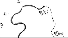
Figure 1: A ribbon represents an SLE trace carrying spin degrees of freedom. Points $z_{i}$ are positions of primary fields. A spin-1/2 operator positioned at the tip extends the trace up to another spin-1/2 operator on the boundary.

At $t=\infty$ the trace hits the boundary and surrounds a critical domain. At any $t<\infty$ one considers the slit domain H_t, i. e. the upper half plane from which the trace is removed (see the figure). The slit domain can be mapped conformally onto the upper half plane by a function $f(z)$ normalized so that $f(z)=z+2t/z+\dots$ near $z=\infty$. The coefficient $t$ is called the capacity of the trace and is chosen to be the time of the evolution. Under this map the tip $z_{t}$ of the trace in the physical plane maps to a point $w_{0}+\xi(t)$ on the real axis. Loewner’s equation connects the evolution of the conformal map $f(z)$ to that of the image $w_{0}+\xi(t)$: $\dot{f}(z)=2/(f(z)-w_{0}-\xi(t))$. It is convenient to shift the map to become $w(z)=f(z)-\xi(t)$, so that the tip is always mapped to the fixed point $w_{0}$ on the real axis of the mathematical plane (coordinate $w$). Then Loewner’s equation becomes

$$dw(z)=\frac{2dt}{w(z)-w_{0}}-d\xi.$$ (1)

In SLE, $\xi(t)$ is a Brownian motion: $\prec\!\dot{\xi}(t)\dot{\xi}(0)\!\!\succ\,=\kappa\delta(t)$. We use the symbol $\prec\!\!...\!\!\succ$ for the stochastic average over the Brownian motion $\xi$ not to be confused with the CFT average $\langle...\rangle$ as e.g. in Eq. (2). Eq. (1) generates a stochastic self-avoiding trace whose statistics is that of a domain wall in a CFT with central charge $c\leqslant 1$, determined by the noise strength $\kappa$ through the relation $c=1-6(\sqrt{\kappa/4}-\sqrt{4/\kappa})^{2}$.

The WZW model

involves a field $G(w,\bar{w})$ taking values in a Lie group. It is a CFT whose action is invariant under independent holomorphic left and anti-holomorphic right multiplication $G\to UGV^{-1}$. It possesses corresponding conserved Noether currents $J_{L}=\partial GG^{-1}$, $J_{R}=-G^{-1}\bar{\partial}G$ which are holomorphic ($J_{L}$) and anti-holomorphic ($J_{R}$). This requires the matrix $G(w,\bar{w})$ to be a product of two holomorphic matrices $G(w,\bar{w})=g^{\vphantom{-1}}_{L}(w)g^{-1}_{R}(\bar{w})$. In terms of these, the currents are expressed as $J_{L}=(\partial g^{\vphantom{-1}}_{L})g^{-1}_{L}$, $J_{R}=(\bar{\partial}g^{\vphantom{-1}}_{R})g_{R}^{-1}$.

Conformal and gauge invariant boundary conditions require that the current normal to the boundary vanishes, i.e. $J_{L}=J_{R}$ on the real axis Cardy (1984); Ishibashi (1989). This condition ‘glues’ holomorphic and anti-holomorphic fields, $g_{L}(w)=g_{R}(w)\Lambda$ (for ${\rm Im}\ w=0$), where $\Lambda$ is a matrix in a Cartan subgroup. As a result, the field $G=g_{R}(w)\Lambda g^{-1}_{R}(\bar{w})$ belongs on the boundary to a conjugacy class (which, in the quantum theory, is quantized) Alekseev:1998mc . For SU(2), conjugacy classes are 2-spheres $S^{2}$ parametrized by a unit vector $\vec{n}$, or points. A boundary condition can be thought of as being associated with a spinIshibashi (1989); Affleck and Ludwig (1991). A change of boundary condition at some point on the real axis can be described by a so-called boundary condition changing operatorCardyNPB1989 which, in the present case, carries spin.

After these comments, consider a critical cluster of a WZW theory. Its boundary is characterized by its fluctuating geometry (the shape of the cluster), which is ‘decorated’ by a spin. Together this can be seen as a self-avoiding walk in the physical plane with a fluctuating spin-1/2 degree of freedom.

The next paragraph recounts arguments which are well described in the SLE literatureSchramm (2000); Lawler book ; Bauer and Bernard (2003). Therefore, we mention only briefly the main steps.

Martingales and Correlation functions in the slit domain.

Let us study correlation functions (conformal blocks) of primary fieldsBPZ ; Knizhnik and Zamolodchikov (1984) of a conformally invariant model, called “spectators”, inserted at points $z_{i}$ in the slit domain H_t made by the trace (see the figure). The positions $z_{i}$ do not move while the trace evolves. Each field $\phi_{\alpha_{i}}(z_{i})$ carries spin $s_{i}$ and conformal weight $h_{i}$ (for a theory with no Lie group symmetry set $s_{i}=0$). We denote by $\psi_{\alpha}$ a boundary condition changing operatorCardyNPB1989 which is also a primary field [for the SU(2) model we choose it to be a spin 1/2 primary field, while for $c<1$ a $(2,1)$ or a $(1,2)$ field in the Kac classification]. Such operators are inserted at the tip and at the end (i.e. at infinity) of the trace.

A bulk operator is the productCardy (1984) of two holomorphic operators located at ‘Schwarz-symmetric’ points as $\phi_{\alpha_{i}}(z_{i})\phi_{\beta_{i}}(z_{i}^{*})$, and transforming in the same representation. An example of a spectator is the matrix $G$ itself. We denote a product of spectators by ${\cal O}(\{z_{i}\})$ and their correlation function in ${\bf H}_{t}$ by ${\cal F}=\langle\alpha|{\cal O}|\beta\rangle_{{\bf H}_{t}}$. In terms of CFT this correlation function reads

$${\cal F}(t,\{z_{i}\})=\frac{\langle\psi^{\dagger}_{\alpha}(\infty)\,{\cal O}\,\psi_{\beta}(z_{t})\rangle_{{\bf H}_{t}}}{(1/2)\langle\psi^{\dagger}_{\gamma}(\infty)\psi_{\gamma}(z_{t})\rangle_{{\bf H}_{t}}}.$$ (2)

It is knownBauer and Bernard (2003) that if we average the correlator (2) in the slit domain over all configurations of the SLE trace, we obtain a CFT correlator in the upper half-plane ${\bf H}$ with the boundary operators inserted:

$$\prec\!\langle\alpha|{\cal O}|\beta\rangle_{{\bf H}_{t}}\!\!\succ =\left\langle\psi^{\dagger}_{\alpha}(\infty)\,{\cal O}\,\psi_{\beta}(w_{0})\right\rangle_{\bf H}.$$ (3)

This implies, as we now review, the steady state condition

$$\partial_{t}\prec\!{\cal F}\!\succ =0.$$ (4)

A stochastic quantity, whose average is time-independent, is known as a ‘martingale’. The argument showing that a correlation function with two boundary operators is a martingale is as follows Bauer and Bernard (2003). At time $t$ we decompose the trace into two parts: one between points $w_{0}$ and $z_{t}$, and the other between $z_{t}$ and infinity (see the figure). We average over all configurations of the trace in two steps. First, we fix the first part and average over the second. Then we average over the first part. The first average can be seen as the CFT average in the slit domain formed by the trace, with two boundary operators inserted, one at the tip of the trace and one at infinity. After performing this (first) average we obtain the quantity in (2). The insertion of the boundary operators effectively averages over the second piece of the domain wall. The second average over the shape of the first part of the trace, as on the l.h.s. of (3) gives us back the original correlator (r.h.s. of that equation). The latter however does not depend on the choice of the midpoint $z_{t}$. Thus the stochastic mean of the correlator ${\cal F}$ is time independent. It is a ‘martingale’.

Stochastic evolution on SU(2) manifold.

In a WZW model we expect not only the geometrical fluctuations due to the growing trace, but also stochastic SU(2) rotations. Accordingly we introduce additional, independent Brownian motions in the left and right su(2) Lie algebras, $\theta_{L,R}=\theta_{L,R}^{a}\,S^{a}$, with variance

$${\prec\!\dot{\theta}_{L,R}^{a}(t)\,\dot{\theta}_{L,R}^{b}(0)\!\!\succ}=\tau\delta^{ab}\delta(t).$$ (5)

Again, we use the symbol $\prec\!\!...\!\!\succ$ for the stochastic average over the Brownian motions $\xi$ and $\theta^{a}$. $S^{a}$ are generators of su(2) in a representation conventionally normalized as $S^{a}S^{a}=s(s+1)$. We define a stochastic evolution in the (complexified) Lie algebra by the equations

$$\Omega_{L} =\frac{d\theta_{L}}{w-w_{0}}, \Omega_{R} =\frac{d\theta_{R}}{{\bar{w}}-w_{0}},$$ (6)

where $\Omega_{L,R}=(dg^{\vphantom{-1}}_{L,R})g^{-1}_{L,R}$, $d\theta_{L,R}=\dot{\theta}_{L,R}\ dt$. Here the time $t$ is the capacity of the trace, and the time derivative is taken at a fixed point $w$ in the mathematical plane. Under this evolution, we let the matrix $G$ itself evolve as $dG=\Omega_{L}G-G\,\Omega_{R}$. These equations respect the form of $G$ as a product of left and right moving factors. The boundary conditions require the left and right Brownian motions to be equal, $\theta_{R}=\theta_{L}$. From now on we will follow only holomorphic components, dropping the index $L$, as if there were no boundary Cardy (1984); Affleck and Ludwig (1991).

The pole in the evolution equation (6) located at the image of the tip of the trace indicates the presence of a source of current $J$ at $w=w_{0}$ in the mathematical plane. This source originates from a juxtaposition of two different gauge invariant boundary conditions to the left and to the right of $w_{0}$. We select the pair of boundary conditions so that the domain wall, located in the physical plane, carries spin 1/2. In the language of boundary CFT, this corresponds to a boundary changing operator, transforming in the spin 1/2 representation, to appear at position $w_{0}$ CardyNPB1989 . The spin 1/2 at the tip of the trace in the physical plane fluctuates during the evolution, and leads to a “twisting” of the domain wall (see the figure).

Making use of the current $J(w)=\partial_{w}GG^{-1}$ in the mathematical plane, the evolution equation (6) can be rewritten in a form where the time derivative is taken at a fixed point in the physical plane:

$$\Omega =\frac{d\theta}{w(z)-w_{0}}+dw(z)J(w(z)).$$ (7)

Under an infinitesimal gauge transformation the current changes as $dJ=[\Omega,J]+\partial_{w}\Omega$. With the help Eqs. (1, 7) we obtain

$$dJ=-\frac{d\theta}{(w-w_{0})^{2}}+\Big{(}\Omega_{A}+h\frac{dw^{\prime}}{w^{\prime}}+\frac{dw}{w^{\prime}}\partial_{z}\Big{)}J.$$ (8)

Here $\Omega_{A}J=[d\theta,J]/(w-w_{0})$ is the adjoint action of the evolution (6), $h=1$ is the conformal weight of the current, and $w^{\prime}=\partial_{z}w(z)$. (8) is a Langevin equation for the current, ressembling [using (1)] the operator product expansion (OPE) of the latter with a primary boundary operator located at the tip.

Langevin equation.

While all the spectator points $z_{i}$ in the physical plane remain fixed under the time evolution, the trace evolves, and together with the infinitesimal rotations this leads to a Langevin dynamics for correlators $\mathcal{F}$ of primary fields, as defined in (2). Using Loewner’s equation (1) and Eq. (6), this is conveniently written through negative grades and global parts of Virasoro and Kac-Moody algebra generators:

$$d{\cal F} =\left(-d\theta^{a}{\cal J}^{a}_{-1}+d\xi\,{\cal L}_{-1}-2dt{\cal L}_{-2}\right){\cal F},$$ (9)

$${\cal L}_{-n} =\sum_{i}\left(\frac{h_{i}(n-1)}{(z_{i}-w_{0})^{n}}-\frac{1}{(z_{i}-w_{0})^{n-1}}\frac{\partial}{\partial z_{i}}\right),\quad n\geqslant-1,$$

$${\cal J}^{a}_{-n} =-\sum_{i}\frac{S^{a}_{i}}{(z_{i}-w_{0})^{n}},\quad n=0,1,\dots$$ (10)

(The sum extends over all spectators and the boundary operator at infinity.) Similarly, the Langevin equation (8) for the current reads, when written in this manner,

$$dJ=d\theta^{a}{\cal J}_{-2}^{a}+\big{(}-d\theta^{a}{\cal J}^{a}_{-1}+d\xi{\cal L}_{-1}-2dt{\cal L}_{-2}\big{)}J,$$ (11)

where now all the generators have the form of Eq. (10) but there is only a single term with $z_{i}\to z$ in the sums.

Diffusion equation.

Let us average the correlator ${\cal F}(t)$ in (2) over all configurations of the fluctuating geometry of the trace and its spin 1/2 degree of freedom. Since the evolution has the form of a Langevin dynamics, the expectation value obeys a diffusion equation. The latter is obtained in the standard manner (see for example, Bauer and Bernard (2003)). We average Eq. (9) over the Gaussain noises. The terms linear in $dt$ come from the first and the second order: $\prec\!d{\cal F}\!\!\succ\,=\bigl{(}\prec\!{\cal G}^{-1}d{\cal G}\!\!\succ+\frac{1}{2}\prec\!({\cal G}^{-1}d{\cal G})^{2}\!\!\succ\bigr{)}$ $\prec\!{\cal F}\!\!\succ$. Here $\cal{G}$ is the time evolution operator, ${\cal G}(t)$, defined by ${\cal F}(t)={\cal G}(t)\,{\cal F}(0)$. One obtains the diffusion equation:

$$\partial_{t}\!\prec\!{\cal F}\!\succ =-H\prec\!{\cal F}\!\succ,\qquad{\rm where}$$ (12)

$$H =-\frac{\kappa}{2}{\cal L}_{-1}^{2}+2{\cal L}_{-2}-\frac{\tau}{2}{\cal J}^{a}_{-1}{\cal J}^{a}_{-1}.$$ (13)

Similarly, we may consider correlators with insertions of the current operator as an additional spectator. Denoting by ${\cal F}_{J}=\langle\alpha|{\cal O}(\{z_{i}\})J(z)|\beta\rangle_{{\bf H_{t}}}$ a correlator of primary fields with an insertion of the current we obtain, with the help of (11), a diffusion-type equation

$$\partial_{t}\prec\!{\cal F}_{J}\!\succ =-H\prec\!{\cal F}_{J}\!\succ-\tau{\cal J}^{a}_{-1}{\cal J}^{a}_{-2}\prec\!{\cal F}\!\succ,$$ (14)

where the last (anomaly) term comes from the first term in Eqs. (8, 11). Here ${\cal J}_{-2}^{a}$ acts only on the position $z$ of the current insertion and ${\cal J}_{-1}^{a}$ on all the spectators apart form the current, while the operators in $H$ act on all spectators, including the current insertion.

Singularity at the tip.

So far the variances $\kappa$ and $\tau$ of the two types of Brownian motion where treated as independent parameters. A simple physical requirement connects them. We may be interested in stochastic processes where martingales (correlation functions) do not have essential singularities as a spectator approaches the tip of the trace. In other words, the singularities of the solutions of the differential equations feature only branch cuts, i.e. the equations are Fuchsian. This occurs only if

$$\kappa+\tau =4.$$ (15)

The simplest way to obtain this condition is to demand that the stochastic average of the one-point function of the current exhibits only a single pole as the current insertion approaches the tip of the trace. Setting ${\cal O}=1$ in (14) we see that the stochastic average of the current one-point function is a zero mode of the operator

$$\frac{\kappa}{2}\partial_{z}^{2}+\frac{\tau}{2}\frac{2}{(z-w_{0})^{2}}+2\partial_{z}\frac{1}{z-w_{0}}.$$ (16)

The requirement that this zero mode be a single pole yields the important condition (15) relating the two variances. It implies in particular that $0\leqslant\kappa\leqslant 4$ since the variance $\tau$ is non-negative; therefore, the trace does not intersect itself Lawler book . [If (15) is not satisfied, one still appears to obtain a possible stochastic process, but with essential singularities in the martingales.]

Knizhnik-Zamolodchikov equation and conformal weight.

The second order differential equation (4,12,13) can be reduced to the first order Knizhnik-Zamolodchikov equationKnizhnik and Zamolodchikov (1984), as we now demonstrate.

Let us denote by $L_{n}$ and $J_{n}$ the Virasoro and the current algebra operators acting on the boundary condition changing operator $\psi(w_{0}):=$ $\psi_{\beta}(w_{0})$ at the tip of the trace. In particular, $L_{0}=h_{0}$, where $h_{0}$ is the conformal weight of $\psi$, $L_{-1}=\partial_{w_{0}}$, and $J_{0}^{a}=\sigma^{a}/2$ acts on the spin 1/2 of $\psi$. The operators in (10) are representations of these operators. Note that $J_{0}^{a}\prec\!{\cal F}\!\succ={\cal J}_{0}^{a}\prec\!{\cal F}\!\succ$ just expresses the invariance of the correlator under global SU(2) transformations. Since the boundary operator $\psi$ is quasiprimaryBPZ , it is annihilated by $L_{1}$. Acting with $L_{1}$ on (4,12,13) yields the first order differential equation

$$\left(L_{-1}-2\gamma{J}^{a}_{-1}J^{a}_{0}\right)\!\prec\!{\cal F}\!\succ =0,$$ (17)

where $2\gamma\!=\!\tau/[6\!-\!(2h_{0}\!+\!1)\kappa]$.​ Acting​ with​ $L_{1}$ again yields​

$$\left(L_{0}-\gamma J^{a}_{0}J^{a}_{0}\right)\!\prec\!{\cal F}\!\succ =0,$$ (18)

which gives $h_{0}=\gamma s(s+1)$, with $s=1/2$ the spin at the tip. We recognize in (17,18) the first two modes of the Sugawara relationKnizhnik and Zamolodchikov (1984). Eq. (17) is the Knizhnik-Zamolodchikov equation arising as a level 1 Null vector of the operator at the tip, and (18) yields the familiar conformal weight of the WZW model Knizhnik and Zamolodchikov (1984).

Finally, if we parametrize $\gamma={1/(k+2)}$, and use the relationship (15) between $\kappa$ and $\tau$, we obtain for $k\neq 1$

$$\tau =\frac{4}{k+3}, \kappa=4\frac{k+2}{k+3}.$$ (19)

The above conditions, however, do not specify $\tau$ and $\kappa$, at $k=1$. The reason for this is that at $k=1$ the WZW model is a CFT with $c=1$, and can be equivalently described in terms of Abelian fields (see below).

In the following paragraph, the parameter $k$ will be identified with the level of the $\text{su}(2)_{k}$ current algebra.

Null vectors.

The action of the operators (10) creates descendant operators of the boundary operator $\psi$ at the tip. Eqs. (4,12,13) mean that $\chi=H\psi$ is a Null vector Knizhnik and Zamolodchikov (1984); BPZ . Acting with ${\cal J}_{1}^{b}$ on (17) shows that the parameter $k$ defined in the last section is the level of the Kac-Moody algebra. Furthermore, acting with ${\cal L}_{2}$ on (4,12,13) expresses the central charge as $c={3\over 4}\tau k+(3\kappa-8)h_{0}$. Inserting $h_{0}=(3/4)/(k+2)$ into the equation appearing in the text below (17), yields a quadratic equation for the level $k$ as a function of $\kappa$ and $\tau$. Thus, both $c$ and $k$ are functions of $\kappa$ and $\tau$. Using (15) one recovers $c=3k/(k+2)$, the familiar central charge of $\text{su}(2)_{k}$.

Relation to unitary minimal models.

As in usual SLE, the variance $\kappa$ alone determines the geometry of the trace. The CFT that describes the geometry of the trace alone corresponds to SLE_κ, with $\kappa$ given by (19). The corresponding portion of central charge is $c_{\kappa}=1-\frac{6}{(k+2)(k+3)}$. We observe that this is the central charge of the minimal unitary model, which can be thought of as the coset model $\text{su}(2)_{k}\oplus\text{su}(2)_{1}/\text{su}(2)_{k+1}$. The remaining part of the central charge, $c_{\tau}=3(k+1)/(k+3)-1$, is the same as that of the coset $\text{su}(2)_{k+1}/\text{u}(1)_{k+1}$ or $Z_{k+1}$ parafermionparafermion . It describes the ‘twisting’ of the trace.

Abelian reduction.

Our stochastic approach is easily specialized to the case of the abelian group U(1). In this case the requirement of Fuchsian singularities that led to Eq. (15) gives the simple condition $\kappa=4$ and eventually leads to $c=1$. Eqs. (4,12,13) still hold but have a different meaning. They are satisfied by a correlator at $c=1$, where the boundary operator has dimension $4h=1-\tau$. By varying $h$ away from $h=1/4$ ($\tau=0$), corresponding to the SU(2) WZW model at level $k=1$, one obtains an evolution which depends both on the geometry and on the U(1) current algebra symmetry. — An analog of (4,12,13) for the Abelian case was obtained in Ref. Cardy (2004) using methods very different from ours.

References

- (1) A. A. Belavin, A. M. Polyakov, and A. B. Zamolodchikov, Nucl. Phys. B241, 333 (1984).
- (2) B. Nienhuis, in Phase transitions and critical phenomena, Vol. 11, Academic Press, London, 1987.
- Schramm (2000) O. Schramm, Israel J. Math 118, 221 (2000).
- (4) G. F. Lawler, Conformally invariant processes in the plane, American Mathematical Society, 2005; W. Werner, ”Random planar curves and Schramm-Loewner evolutions”, in Lecture Notes in Mathematics, 1840, Springer, 2004.
- (5) For a recent review see: J. Cardy, Annals Phys. 318, 81 (2005) cond-mat/0503313.
- Bauer and Bernard (2003) M. Bauer and D. Bernard, Commun. Math. Phys. 239, 493 (2003); eprint cond-mat/0412372.
- Knizhnik and Zamolodchikov (1984) V. G. Knizhnik and A. B. Zamolodchikov, Nucl. Phys. B247, 83 (1984).
- (8) I. Affleck and F. D. M. Haldane, Phys. Rev. B36, 5291 (1987).
- (9) P. Nozières and A. Blandin, J. Phys. Paris 41, 193 (1980).
- (10) A. Y. Alekseev and V. Schomerus Phys. Rev. D60, 061901 (1999); G. Felder et al., J. Geom. Phys. 34, 162 (2000); V. Schomerus, Class. Quantum Grav. 19, 5781 (2002).
- (11) J. Kondev, C. L. Henley, Nucl. Phys. B464, 540 (1996), J. Kondev, Int. J. Mod. Phys. B11, 153 (1997); N. Read, reported at Kagomé Workshop (Jan. 1992), unpublished.
- (12) A very different approach was suggested in J. Rasmussen, hep-th/0409026.
- Cardy (1984) J. L. Cardy, Nucl. Phys. B240, 514 (1984).
- Ishibashi (1989) N. Ishibashi, Mod. Phys. Lett. A4, 251 (1989).
- Affleck and Ludwig (1991) I. Affleck and A. W. W. Ludwig, Nucl. Phys. B352, 849 (1991); Nucl. Phys. B428, 545 (1994).
- (16) J. L. Cardy, Nucl. Phys. B324, 581 (1989); I. Affleck and A. W. W. Ludwig, J. Phys. A27, 5375 (1994).
- (17) A. B. Zamolodchikov, V.A. Fateev, JETP 62 (1985), 215.
- Cardy (2004) J. Cardy (2004), eprint math-ph/0412033.