IMSC/2005/03/01
Aspects of Open-Closed Duality in a Background $B$-Field

Abstract

We study closed string exchanges in background $B$-field. By analysing the two point one loop amplitude in bosonic string theory, we show that tree-level exchange of lowest lying, tachyonic and massless closed string modes, have IR singularities similar to those of the nonplanar sector in noncommutative gauge theories. We further isolate the contributions from each of the massless modes. We interpret these results as the manifestation of open/closed string duality, where the IR behaviour of the boundary noncommutative gauge theory is reconstructed from the bulk theory of closed strings.

1 Introduction

Dynamics of strings in background fields is an old subject. Open string dynamics in background two form field is an interesting area giving rise to various new phenomena. Specifically the study of open strings in the presence of background constant two from $B$-field has shown how noncommutative spacetimes can arise in string theory [1, 2, 3, 4]. By switching on a constant $B$-field along the world-volume directions of a $D$-brane, it was shown that spacetime coordinates along these directions no longer commute. The low energy dynamics of the $D$-brane is described by a noncommutative Yang-Mills theory. Noncommutative gauge theories and noncommutative versions of other field theories have since been studied extensively for the past few years. For reviews on the subject see [5]. These field theories are a class of nonlocal theories, but are tractable and offer new interesting phenomena that are closely related to the parent string theory.

A generic characteristic of noncommutative field theories is the mixing of the UV and IR regimes arising in the nonplanar sectors [6]. A lot of effort by various authors have been made to understand this interesting feature. Usual notions of Wilsonian RG do not fit in the continuum limit. Contradictory, as this may seem in the field theoretic picture, this phenomenon has a natural interpretation in string theory. Open string one loop amplitudes have a dual description in terms of tree-level propagation of closed string modes. The UV region of the open string loop, in the dual picture is dominated by the lightest closed string modes. The UV divergences of the open string loop can thus be reinterpreted as IR divergences due to propagating massless closed string modes. Though attempts have been made along these lines to understand the IR divergences occurring in noncommutative field theories by integrating out high energy degrees of freedom [14, 15], the picture still remains unclear. See also [16]. We address this issue in this paper. In the bosonic string theory setting, we first analyse the two-point one loop amplitude for gauge bosons on the brane, in the closed string channel. We argue that the region of the modulus giving rise to divergences (that are regulated in the nonplanar amplitudes) in noncommutative field theories can be identified as the region where the lightest closed string modes dominate in the dual picture. In usual quantum field theory, because of infinities, there is no way to compare quantitatively the contributions in these two pictures. In the presence of the background $B$-field the nonplanar diagrams are regulated and a quantitative approach can thus be made. The full two point open string amplitude also contains finite contributions which would require the entire tower of closed string states for its dual description. However, the singular IR behaviour of the nonplanar amplitudes, in the boundary noncommutative gauge theory can be seen from the exchange of closed strings in the bulk. On the broader side, these results can be seen from the point of view of open/closed string duality. This is similar in spirit to the AdS/CFT correspondence [8]. Here the bulk theory of closed strings is in flat space, but in the presence of constant background $B$-field.

Though there are additional tachyonic divergences, we are able to show that the form of IR divergences with appropriate tensor structures can be extracted by considering only lowest lying modes (tachyonic and massless). We further analyse the two point amplitude by studying massless closed string exchanges in background constant $B$-field. From this analysis we are able to isolate the individual contributions from the massless closed string exchanges.

This paper is organised as follows. In section 2, we review concisely, the open string dynamics in the presence of background constant $B$-field and the arising of noncommutative field theory in the Seiberg-Witten limit. In section 3, we study the one loop open string amplitude in the UV limit and write down the contribution from the lowest states. In section 4, we analyse massless closed string exchange in background $B$-field and reconstruct the massless contribution computed in section 3. In section 5, we conclude with discussions and further prospects.

Conventions: We will use capital letters $(M,N,...)$ to denote general spacetime indices and small letters $(i,j,...)$ for coordinates along the $D$-brane. Small Greek letters $(\alpha,\beta...)$ will be used to denote indices for directions transverse to the brane.

2 Open strings in background $B$-field

In this section we give a short review of open string dynamics in the presence of constant background $B$-field leading to noncommutative field theory on the world volume of a $D$-brane [4]. In the presence of a constant background $B$-field, the world sheet action is given by,

$$S=\frac{1}{4\pi\alpha^{{}^{\prime}}}\int_{\Sigma}[g_{MN}\partial_{a}X^{M}\partial^{a}X^{N}-2\pi i\alpha^{{}^{\prime}}B_{MN}\epsilon^{ab}\partial_{a}X^{M}\partial_{b}X^{N}]$$ (1)

Consider a $D_{p}$ brane extending in the directions $1$ to $p$, such that, $B_{MN}\neq 0$ only for $M,N\leq p+1$ and $g_{MN}=0$ for $M\leq p+1,N>p$. The equation of motion gives the following boundary condition,

$$g_{MN}\partial_{n}X^{N}+2\pi i\alpha^{{}^{\prime}}B_{MN}\partial_{t}X^{N}|_{\partial\Sigma}=0$$ (2)

The world sheet propagator on the boundary of a disc satisfying this boundary condition is given by,

$${\cal G}(y,y^{{}^{\prime}})=-\alpha^{{}^{\prime}}G^{MN}\ln(y-y^{{}^{\prime}})^{2}+\frac{i}{2}\theta^{MN}\epsilon(y-y^{{}^{\prime}})$$ (3)

where, $\epsilon(\Delta y)$ is $1$ for $\Delta y>0$ and $-1$ for $\Delta y<0$. $G_{MN}$, $\theta_{MN}$ are given by,

$$G^{MN} = \left(\frac{1}{g+2\pi\alpha^{{}^{\prime}}B}g\frac{1}{g-2\pi\alpha^{{}^{\prime}}B}\right)^{MN}$$

$$G_{MN} = g_{MN}-(2\pi\alpha^{{}^{\prime}})^{2}(Bg^{-1}B)_{MN}$$

$$\theta^{MN} = -(2\pi\alpha^{{}^{\prime}})^{2}\left(\frac{1}{g+2\pi\alpha^{{}^{\prime}}B}B\frac{1}{g-2\pi\alpha^{{}^{\prime}}B}\right)^{MN}$$ (4)

The relations above define the open string metric $G$ in terms of the closed string metric $g$ and $B$. This difference in the two metrics as seen by the open strings on the brane and the closed strings in the bulk plays an important role in the discussions in the following sections. We next turn to to the low energy limit, $\alpha^{{}^{\prime}}\rightarrow 0$. A nontrivial low energy theory results from the following scaling.

$$\alpha^{{}^{\prime}}\sim\epsilon^{1/2}\rightarrow 0\mbox{\hskip 7.22743pt;\hskip 7.22743pt}g_{ij}\sim\epsilon\rightarrow 0$$ (5)

where, $i,j$ are the directions along the brane. This is the Seiberg Witten (SW) limit which gives rise to noncommutative field theory on the brane. The relations in eqn(2), to the leading orders, in this limit reduce to,

$$G^{ij} = -\frac{1}{(2\pi\alpha^{{}^{\prime}})^{2}}(\theta g\theta)^{ij}\mbox{\hskip 7.22743pt;\hskip 7.22743pt}G_{ij}=-(2\pi\alpha^{{}^{\prime}})^{2}(Bg^{-1}B)_{ij}$$

$$\theta^{ij} = \left(\frac{1}{B}\right)^{ij}$$ (6)

for directions along the $D_{p}$ brane. $G_{MN}=g_{MN}$ and $\theta=0$ otherwise. It was shown that the tree-level action for the low energy effective field theory on the brane has the following form,

$$S_{YM}=-\frac{1}{g_{YM}^{2}}\int\sqrt{G}G^{kk^{{}^{\prime}}}G^{ll^{{}^{\prime}}}\mbox{Tr}(\hat{F}_{kl}*\hat{F}_{k^{{}^{\prime}}l^{{}^{\prime}}})$$ (7)

where the $*$-product is defined by,

$$f*g(x)=e^{\frac{i}{2}\theta^{ij}\partial_{i}^{y}\partial_{j}^{z}}f(y)g(z)\mid_{y=z=x}$$ (8)

and $\hat{F}_{kl}$ is the noncommutative field strength, which is related to the ordinary field strength, $F_{kl}$ by,

$$\hat{F}_{kl}=F_{kl}+\theta^{ij}(F_{ki}F_{lj}-A_{i}\partial_{j}F_{kl})+{\cal O}(F^{3})$$ (9)

and,

$$\hat{F}_{kl}=\partial_{k}\hat{A}_{l}-\partial_{l}\hat{A}_{k}-i\hat{A}_{k}*\hat{A}_{l}+i\hat{A}_{l}*\hat{A}_{k}$$ (10)

Noncommutative field theories as defined here have been studied extensively for the last few years. One of the most important features of these theories is the coupling of the UV and the IR regimes, manifested by the nonplanar sector of these theories, contradicting our usual notions of Wilsonian RG [6]. This mixing of the UV and IR sectors also occurs in scalar theories, where the noncommutative version is formulated by replacing all products of fields by $*$-products. We write down here a simple two point nonplanar one loop amplitude for noncommutative $\phi^{4}$ theory in four dimensions, in the continuum limit,

$$\Gamma^{2}(p)\sim\frac{1}{\tilde{p}^{2}}-m^{2}\ln(\tilde{p}^{2}m^{2})$$ (11)

where, $\tilde{p}=(\theta p)$. The amplitude is finite in the UV but is IR divergent though we had a massive theory to start with. Note that $\tilde{p}^{2}$ plays the role of $1/\Lambda^{2}$, where $\Lambda$ is the UV cutoff. It was suggested [6] that these IR divergent terms could arise by integrating out massless modes at high energies. This is quite like the open string one loop divergence which is reinterpreted as IR divergence coming from massless closed string exchange. It was noted that the first and second terms of eqn(11) can be recovered through massless tree-level exchanges if these modes are allowed to propagate in $0$ and $2$ extra dimensions transverse to the brane respectively [7]. A similar structure arises for the nonplanar two point function for the gauge boson in noncommutative gauge theories,

$$\Pi^{ij}(p)\sim N_{1}[G^{ij}G^{kl}-G^{ik}G^{jl}]p_{k}p_{l}\ln(p^{2}\tilde{p}^{2})+N_{2}\frac{\tilde{p}^{i}\tilde{p}^{j}}{\tilde{p}^{4}}$$ (12)

$N_{1}$ and $N_{2}$ depends on the matter content of the theory. For some early works on noncommutative gauge theories see [9]. The effective action with the two point function (12) is not gauge invariant. To write down a gauge invariant effective action one needs to introduce open Wilson lines [10]

$$W_{C}(p)=\int d^{4}xP*\exp\left(ig\int_{C}d\sigma\partial_{\sigma}y^{i}A_{i}(x+y(\sigma)\right)*e^{ipx}$$ (13)

The curve $C$ is parametrized by $y^{i}(\sigma)$, where $0\leq\sigma\leq 1$ such that, $y^{i}(1)-y^{i}(0)=\tilde{p}^{i}$. Correlators of Wilson lines in noncommutative gauge theories have been studied by various authors [11]. The terms in (12) are the leading terms in the expansion of the two point function for the open Wilson line. A crucial point to be noted is that for supersymmetric theories, $N_{2}$, the coefficient of the second term, which is allowed by the noncommutative gauge invariance vanishes [12]. Also see [13] for an elaborate discussion. An observation on the arising of tachyon in the closed string theory in the bulk and the non vanishing of $N_{2}$ was made in [17]. Attempts have been made, along the lines as discussed above, to recover the nonplanar IR divergent terms from tree-level closed string exchanges. We analyse this issue in the next section.

3 Open string one loop amplitude

In this section we compute the open string one loop amplitude with insertion of two gauge field vertices. We will compute the two point amplitude in the closed string channel keeping only the contributions from the tachyon and the massless modes. One loop amplitudes for open strings with two vertex insertions in the presence of a constant background $B$-field have been computed by various authors, and field theory amplitudes were obtained in the $\alpha^{{}^{\prime}}\rightarrow 0$ limit [14].

Firstly, the one loop partition function is written as [21, 20]

$$Z(t)=\det(g+2\pi\alpha^{{}^{\prime}}B)Z_{0}(t)$$ (14)

with,

$$Z_{0}(t)=\mbox{Tr}[\exp(-2\pi tL_{0})]$$ (15)

where, $t$ is the modulus of the cylinder and $L_{0}$ is given by,

$$L_{0}=\alpha^{{}^{\prime}}G_{ij}k^{i}k^{j}+\frac{(X^{\alpha})^{2}}{4\pi^{2}\alpha^{{}^{\prime}}}+\frac{1}{2}\sum_{q\neq 0}G_{MN}a_{q}^{M}a_{-q}^{N}$$ (16)

For an open string ending on a $D_{p}$ brane ($X^{\alpha}=0$), this gives,

$$Z(t)=\det(g+2\pi\alpha^{{}^{\prime}}B){\cal V}_{p+1}(8\pi^{2}\alpha^{{}^{\prime}}t)^{-\frac{p+1}{2}}\eta(it)^{-(D-2)}$$ (17)

${\cal V}_{p+1}$ is the volume of the $D_{p}$ brane. We are interested in the two point one loop amplitude. Specifically we write down here the nonplanar amplitude for reasons mentioned earlier. The two point one loop amplitude has the form,

$$A(p_{1},p_{2})=\int_{0}^{\infty}\frac{dt}{2t}Z(t)\int_{0}^{2\pi t}dy\int_{0}^{2\pi t}dy^{{}^{\prime}}<V(p_{1},x,y)V(p_{2},x^{{}^{\prime}},y^{{}^{\prime}})>$$ (18)

where $Z(t)$ is as defined in eqn(17). The required vertex operator is given by,

$$V(p,y)=-i\frac{g_{o}}{(2\alpha^{{}^{\prime}})^{1/2}}\epsilon_{j}\partial_{y}X^{j}e^{ip.X}(y)$$ (19)

The noncommutative field theory results are recovered from region of the modulus where $t\rightarrow\infty$ in the SW limit. As mentioned, the nonplanar diagrams in the noncommutative field theory gives rise to terms which manifest coupling of the UV to the IR sector of the field theory.

The $t\rightarrow 0$ limit, picks out the contributions only from the tree-level massless closed string exchange. This is the UV limit of the open string. The amplitude is usually divergent. However, in the usual case, these divergences are reinterpreted as IR divergences due to the massless closed string modes. What is the role played by the $B$-field? In the presence of the background $B$-field, the integral over the modulus is regulated. In the closed string side, this would mean that the propagator for the massless modes are modified so as to remove the IR divergences. We would now like to investigate this end of the modulus.

Before going into the actual form let us see heuristically what we can expect to compare on both ends of the modulus. First consider the one loop amplitude,

$${\cal Z}\sim\int\frac{dt}{t}(\alpha^{{}^{\prime}}t)^{-\frac{p+1}{2}}\eta(it)^{-(D-2)}\exp(-C/\alpha^{{}^{\prime}}t)$$ (20)

where $C$ is some constant which in our case is dependent on the $B$-field. In the $t\rightarrow\infty$ limit,

$${\cal Z}_{op}\sim\int\frac{dt}{t}(\alpha^{{}^{\prime}}t)^{-\frac{p+1}{2}}\left[e^{2\pi t}+(D-2)+O(e^{-2\pi t})\right]\exp(-C/\alpha^{{}^{\prime}}t)$$ (21)

If we throw out the tachyon, and restrict ourselves only to the $O(1)$ term in the expansion of the $\eta$-function, $\alpha^{{}^{\prime}}$ and $t$ occur in pairs. This means that in the $\alpha^{{}^{\prime}}\rightarrow 0$ limit the finite contributions to the field theory come from the region where $t$ is large. We can break the integral over $t$ into two parts, $1/\Lambda^{2}\alpha^{{}^{\prime}}<t<\infty$ and $0<t<1/\Lambda^{2}\alpha^{{}^{\prime}}$, where $\Lambda$ translates into the UV cutoff for the field theory on the brane. The second interval is the source of divergences in the field theory that is regulated by $C$. This is the region of the modulus dominated by massless exchanges in the closed string channel. For the closed string channel, we have

$${\cal Z}_{cl}\sim\int ds(\alpha^{{}^{\prime}})^{-\frac{p+1}{2}}s^{-l/2}\left[e^{2\pi s}+(D-2)+O(e^{-2\pi s})\right]\exp(-Cs/\alpha^{{}^{\prime}})$$ (22)

where $l=D-(p+1)$, is the number of dimensions transverse to the $D_{p}$ brane. The would be divergences as $C\rightarrow 0$ manifest themselves as $1/C$ or $\ln(C)$, depending on $l$ [7]. The full open string channel result will always require all the closed string modes for its dual description. As far as the divergent (UV/IR mixing) terms are concerned, we can hope to realise them through some field theory of the massless closed string modes. However, the exact correspondence between the divergences in both the channels, is destroyed by the presence of the tachyons. Also note that, at the $t\rightarrow 0$ end of the open string one loop amplitude, the divergence is contributed by the full tower of open string modes. However, we want that the one loop open string amplitude restricted to only the massless exchanges to be rewritten as massless closed string exchanges. For this to happen the integrand as a function of $t$ in one loop amplitude should have the same asymptotic form as $t\rightarrow 0$ and $t\rightarrow\infty$ so that eqn(22) is exactly the same as that of eqn(21) integrated between $[0,1/\Lambda^{2}\alpha^{{}^{\prime}}]$. There are examples of supersymmetric configurations where the one loop open string amplitude restricted to the massless sector can be rewritten exactly as tree-level massless closed string exchanges. It was shown that in these situations the potential between two branes with separation $r$ is the same at both the $r\rightarrow 0$, and $r\rightarrow\infty$ corresponding to $t\rightarrow\infty$ and $t\rightarrow 0$ ends respectively [18]. Consequences of this fact in relation to the gauge/gravity correspondence have been explored in [19]. We can expect that in these cases the IR singularities of the noncommutative gauge theory match with those computed from the closed string massless exchanges. In the bosonic case, this is true for $p=13$, if we remove the tachyons. However, we are concerned with reproducing UV/IR effects of four dimensional gauge theory for which we need to set $l=2$. The broader purpose of the exercise that follows is to outline a construction that can be set up for supersymmetric cases.

We now return to the original computation of the amplitude in the closed string channel. The nonplanar world sheet propagator obtained by restricting to the positions at the two boundaries is [20, 14],

$${\cal G}^{ij}(y,y^{{}^{\prime}})=-\alpha^{{}^{\prime}}G^{ij}\ln\left|e^{-\frac{\pi}{4t}}\frac{\vartheta_{4}\left(\frac{\Delta y}{2\pi t},\frac{i}{t}\right)}{t^{-1}\eta(i/t)^{3}}\right|^{2}-i\frac{\theta^{ij}\Delta y}{2\pi t}-\alpha^{{}^{\prime}}g^{ij}\frac{\pi}{2t}$$ (23)

where, $\Delta y=y-y^{{}^{\prime}}$. In the limit $t\rightarrow 0$ the propagator has the following structure,

$${\cal G}^{ij}=-4\alpha^{{}^{\prime}}G^{ij}\left[cos(\Delta y/t)e^{-\frac{\pi}{t}}-e^{-\frac{2\pi}{t}}\right]-i\frac{\theta^{ij}\Delta y}{2\pi t}-\alpha^{{}^{\prime}}g^{ij}\frac{\pi}{2t}$$ (24)

Inserting this into the correlator for two gauge bosons and keeping only terms that would contribute to the tachyonic and massless closed string exchanges, we get,

$$<...>=\left[p_{k}p_{l}\frac{(8\pi\alpha^{{}^{\prime}})^{2}}{(2\pi t)^{2}}(G^{ij}G^{kl}-G^{ik}G^{jl})sin^{2}(\Delta y/t)e^{-\frac{2\pi}{t}}+\frac{\tilde{p}^{i}\tilde{p}^{j}}{(2\pi t)^{2}}\right]e^{p_{i}{\cal G}^{ij}p_{j}}$$ (25)

expanding $\eta(it)$ in this limit,

$$\eta(it)^{-(D-2)}=t^{\frac{D-2}{2}}\eta(i/t)^{-(D-2)} \sim t^{\frac{D-2}{2}}[e^{\frac{2\pi}{t}}+(D-2)+O(e^{-\frac{2\pi}{t}})]$$ (26)

The two point amplitude with only the tachyonic and the massless closed string exchange can now be written down,

$$A_{2}(p,-p)=-i\det(g+2\pi\alpha^{{}^{\prime}}B){\cal V}_{p+1}(\frac{g_{o}^{2}}{2\alpha^{{}^{\prime}}})(8\pi^{2}\alpha^{{}^{\prime}})^{-\frac{p+1}{2}}\epsilon_{i}\epsilon_{j}I(p)$$ (27)

with $I(p)=I_{T}(p)+I_{\chi}(p)$ and,

$$I_{T}(p) = \tilde{p}^{i}\tilde{p}^{j}\int dss^{-\frac{l}{2}}\exp\left\{-(\frac{\alpha^{{}^{\prime}}\pi}{2}p_{i}g^{ij}p_{j}-2\pi)s\right\}$$

$$= 4\pi(2\pi^{2}\alpha^{{}^{\prime}})^{\frac{l}{2}-1}\tilde{p}^{i}\tilde{p}^{j}\int\frac{d^{l}k_{\perp}}{(2\pi)^{l}}\frac{1}{k_{\perp}^{2}+p_{i}g^{ij}p_{j}-4/\alpha^{{}^{\prime}}}$$

We have written the integral over $t$ in terms of $s=1/t$ in (3) and further in the last expression we have replaced the integral over $s$ with that of $k_{\perp}$. The dimension of the $k_{\perp}$ integral is the number of directions transverse to the brane and is thus the momentum of the closed string along these directions. Note that the $s$ integral has to be cutoff at the lower end at some value $\Lambda^{2}\alpha^{{}^{\prime}}$. This corresponds to the UV transverse momentum cutoff for the closed strings, that allows us to extract the contribution from the IR region.

$$I(p,\Lambda)\sim\int_{\Lambda^{2}\alpha^{{}^{\prime}}}^{\infty}\frac{ds}{s}e^{-p^{2}\alpha^{{}^{\prime}}s}\sim\int_{0}^{\infty}d^{2}k_{\perp}\frac{e^{-(k_{\perp}^{2}+p^{2})\Lambda^{2}\alpha^{{}^{\prime}2}}}{(k_{\perp}^{2}+p^{2})\alpha^{{}^{\prime}}}$$ (29)

The integral over $k_{\perp}$, eqn(29) receives contribution upto $k_{\perp}\sim O(1/\Lambda\alpha^{{}^{\prime}})$. The included region of the $k_{\perp}$ integral is the required IR sector for the transverse closed string modes or the UV for the open string channel. With this observation, for the tachyon with $l=2$, we get

$$I_{T}(p,\Lambda) = 4\pi^{2}(2\pi^{2}\alpha^{{}^{\prime}})^{\frac{l}{2}-1}\tilde{p}^{i}\tilde{p}^{j}\ln\left(\frac{p_{i}g^{ij}p_{j}-4/\alpha^{{}^{\prime}}+\frac{1}{(\Lambda\alpha^{{}^{\prime}})^{2}}}{p_{i}g^{ij}p_{j}-4/\alpha^{{}^{\prime}}}\right)$$ (30)

For the noncommutative limit (5), we can expand the answer (30) in powers of $1/(\alpha^{{}^{\prime}}pg^{-1}p)$,

$$\ln\left(pg^{-1}p-4/\alpha^{{}^{\prime}}\right)\sim\ln\left(pg^{-1}p\right)-\frac{4}{\alpha^{{}^{\prime}}pg^{-1}p}-\frac{1}{2}\left(\frac{4}{\alpha^{{}^{\prime}}pg^{-1}p}\right)^{2}-\textellipsis$$ (31)

The $(1/\alpha^{{}^{\prime}}pg^{-1}p)^{2}$ term in the expansion (31) above corresponds to the IR singular term which appears in the noncommutative gauge theory. To compare with the second term of (12), we should set $G=\eta$, so that $g^{-1}\sim-\theta^{2}/\alpha^{{}^{\prime}2}$. Here we have got this from one of the terms in the expansion of the amplitude with tachyon exchange. However one can easily see that any massive spin zero closed string exchange would produce such a term. As far as the exact coefficient is concerned, the full tower of massive states would contribute. The absence of this term in the supersymmetric theories can only be due to exact cancellations between the bosonic and fermionic sector contributions [17].

As for the tachyon, similarly we now write down the contribution from the massless exchanges,

$$I_{\chi}(p,\Lambda) = 4\pi(2\pi^{2}\alpha^{{}^{\prime}})^{\frac{l}{2}-1}\left[(D-2)\tilde{p}^{i}\tilde{p}^{j}+8(2\pi\alpha^{{}^{\prime}})^{2}p_{k}p_{l}(G^{ij}G^{kl}-G^{ik}G^{jl})\right]\times$$ (32)

$$\times \int\frac{d^{l}k_{\perp}}{(2\pi)^{l}}\frac{1}{k_{\perp}^{2}+p_{i}g^{ij}p_{j}}$$

One can observe that the terms occurring with $\alpha^{{}^{\prime}2}(\sim\epsilon)$ as the coefficient, relative to the other terms in (31) and (32), appear in the gauge theory result in eqn(12). In the closed string channel we have got this for the number of transverse dimensions, $l=2$. This means that $p+1=D-2=24$ is the dimension of the gauge theory on the string side. However the result of eqn(12) is valid for the NC gauge theory defined in 4-dimensions. To understand why it is these terms that occur in the four dimensional gauge theory, we must have a string setting where $l=2$ and $p=3$. However, at this point, as discussed earlier, it is only necessary that $l=2$ so that the lowest lying closed string exchanges reproduce the correct form of the IR singularities as that of the gauge theory in eqn(12).

We mention again that the exact correspondence between the UV behavior of the noncommutative gauge theory and closed string exchanges would require the full tower of closed string states. The contribution from the massive closed string states are likely to be supressed only in some supersymmetric configurations [18][19]. Keeping in mind these situations we compute the exchanges due to massless closed strings in the presence of background $B$-field in the following section.

4 Closed string exchange

In this section we reconstruct the two point function of two gauge fields eqn(32) with massless closed string exchanges. The aim here is to write the amplitude as sum of massless closed string exchanges in the presence of constant background $B$-field. To proceed, by considering the effective field theory of massless closed strings, we construct the propagators for these modes (graviton, dilaton and $B$-field) with a constant background $B$-field. As a next step we compute the couplings of the gauge field on the brane with the massless closed strings from the DBI action. Finally we combine these results to construct the two point function. We will consider three separate cases when computing the two point amplitude in this section. (I) In this case the background $B$ field is assumed to be small and the closed string metric, $g=\eta$. (II)The Seiberg Witten limit when $g=\epsilon\eta$. (III)The case when the open string metric on the brane, $G=\eta$. The amplitude eqn(32) in the closed string channel is the closed form result of the massless exchanges. In each of the above cases, we will compare this amplitude to respective orders with the ones we compute here in this section. Let us first begin by considering the field theory of the massless modes of the closed string string propagating in the bulk. The spacetime action for closed string fields is written as,

$$S=\frac{1}{2\kappa^{2}}\int d^{D}X\sqrt{-g}[R-\frac{1}{12}e^{-\frac{8\phi}{D-2}}H_{LMN}H^{LMN}-\frac{4}{D-2}g^{MN}\partial_{M}\phi\partial_{N}\phi]$$ (33)

Where $D$ is the number of dimensions in which the closed string propagates. The indices are raised and lowered by $g$. We will now construct the tree-level propagators that will be necessary in the next section to compute two point amplitudes. For each of the cases as defined above, the propagator will take a different form. Let us first consider the dilaton. For $g=\eta$ the propagator is the usual one,

$$<\phi\phi> = -\frac{(D-2)i\kappa^{2}}{4}\frac{1}{k_{\perp}^{2}+k_{\parallel}^{2}}$$ (34)

The next limit for the metric is $g=\epsilon\eta$ along the world volume directions of the brane. In this limit, the dilaton part of the action can be written as,

$$S_{\phi}=-\frac{4}{\kappa^{2}(D-2)}\int d^{D}X\frac{1}{2}[\partial_{\alpha}\phi\partial^{\alpha}\phi+\epsilon^{-1}\partial_{i}\phi\partial^{i}\phi]$$ (35)

This gives the propagator,

$$<\phi\phi> = -\frac{(D-2)i\kappa^{2}}{4}\frac{1}{k_{\perp}^{2}+\epsilon^{-1}k_{\parallel}^{2}}$$ (36)

Finally, when the open string metric is set to, $G=\eta$, the lowest order solution for $g$ along the brane directions is,

$$g=-(2\pi\alpha^{{}^{\prime}})^{2}B^{2}+{\cal O}(\alpha^{{}^{\prime}4})$$ (37)

which gives,

$$<\phi\phi> = -\frac{(D-2)i\kappa^{2}}{4}\frac{1}{k_{\perp}^{2}+\tilde{k_{\parallel}}^{2}/(2\pi\alpha^{{}^{\prime}})^{2}}$$ (38)

where,

$$\tilde{k_{\parallel}}^{2}=-k_{\parallel i}\left(\frac{1}{B^{2}}\right)^{ij}k_{\parallel j}$$ (39)

Let us now turn to the free part for the antisymmetric tensor field,

$$S_{b}=-\frac{1}{24\kappa^{2}}\int d^{D}XH_{LMN}H^{LMN}$$ (40)

where,

$$H_{LMN}=\partial_{L}b_{MN}+\partial_{M}b_{NL}+\partial_{N}b_{LM}$$ (41)

Using the following gauge fixing condition,

$$g^{MN}\partial_{M}b_{NL}=0$$ (42)

The action reduces to,

$$S_{b}=-\frac{(2\pi\alpha^{{}^{\prime}})^{2}}{8\kappa^{2}}\int d^{D}X\left[g^{\alpha\beta}\partial_{\alpha}b_{IJ}\partial_{\beta}b_{KL}+g^{ij}\partial_{i}b_{IJ}\partial_{j}b_{KL}\right]g^{IK}g^{JL}$$ (43)

The factor of $(2\pi\alpha^{{}^{\prime}})^{2}$ in the $b$-field action has been included because the sigma model is defined with $(2\pi\alpha^{{}^{\prime}})B$ coupling. The propagator then is,

$$<b_{IJ}b_{I^{{}^{\prime}}J{{}^{\prime}}}>=-\frac{2i\kappa^{2}}{(2\pi\alpha^{{}^{\prime}})^{2}}\frac{g_{I[J{{}^{\prime}}}g_{I^{{}^{\prime}}]J}}{k_{\perp}^{2}+g^{ij}k_{\parallel i}k_{\parallel j}}$$ (44)

Finally, the gravitational part of the action. As will turn out in the next section that we will only have to consider graviton exchanges for the case $g=\eta$. The propagator for the graviton here is the usual propagator from the action,

$$S_{h}=\frac{1}{2\kappa^{2}}\int d^{D}X\sqrt{-g}R$$ (45)

By considering fluctuations about $\eta$, and in the gauge (47),

$$g_{MN}=\eta_{MN}+h_{MN}$$ (46)

$$g^{MN}\Gamma^{L}_{MN}=0$$ (47)

the graviton propagator is,

$$<h_{IJ}h_{I^{{}^{\prime}}J{{}^{\prime}}}>=-2i\kappa^{2}\frac{[\eta_{I\{J{{}^{\prime}}}\eta_{I^{{}^{\prime}}\}J}-2/(D-2)\eta_{IJ}\eta_{I^{{}^{\prime}}J{{}^{\prime}}}]}{k_{\perp}^{2}+k_{\parallel}^{2}}$$ (48)

After writing down the required propagators, we now turn to the computation of the vertices. As mentioned in the beginning of this section, we will consider each of the three cases separately. To begin, we first write down the DBI action for a $D_{p}$ brane,

$$S_{p}=-T_{p}\int d^{p+1}\xi e^{-\Phi}\sqrt{g^{{}^{\prime}}+2\pi\alpha^{{}^{\prime}}(B+b)}$$ (49)

Where, $g^{{}^{\prime}}$ is the closed string metric in the string frame, $B$ is the constant two form background field and $b$ is the fluctuation of the two form field. The $b$-field on the brane is interpreted as the two form field strength for the $U(1)$ gauge field and in the bulk it is the usual two form potential. Going to the Einstein frame by defining,

$$g=g^{{}^{\prime}}e^{2\omega}\mbox{;\hskip 14.45377pt}\omega=\frac{2(\phi_{0}-\Phi)}{D-2}\mbox{;\hskip 14.45377pt}\Phi=\phi+\phi_{0}\mbox{;\hskip 14.45377pt}\omega=\frac{-2\phi}{D-2}$$ (50)

the action can be rewritten as,

$$S_{p}= - \tau_{p}\int d^{p+1}\xi{\cal L}(\phi,,h,b)$$ (51)

$$- \tau_{p}\int d^{p+1}\xi e^{-\phi(1-\frac{2(p+1)}{D-2})}\sqrt{g+2\pi\alpha^{{}^{\prime}}(B+b)e^{-\frac{4\phi}{D-2}}}$$

where, $\tau_{p}=T_{p}e^{-\phi_{0}}$ and $\phi$ is the propagating dilaton field. We will now consider each of the three cases separately and compute the two point function upto the respective orders.

4.1 Expansion for small $B$

In this part we compute the couplings of the gauge field on the brane to the massless closed strings in the bulk. We will assume the background constant $B$-field to be small and compute the lowest order contribution to the two point function considered as an expansion in $B$. The first thing to note is that, since $B$ is antisymmetric, there cannot be a non vanishing amplitude with a single $B$ in one vertex only. We need at least two powers of $B$. One on each vertex or both on one. The graviton and the dilaton need one on each vertex. The $b$-field can couple to the gauge field without a $B$. So for the $b$-field we need to consider couplings upto ${\cal O}(B^{2})$. The closed string tree-level diagrams contributing to the three massless modes are shown in Figure 1.

$${\cal L}=\sqrt{e^{-P\phi}\left[g+(2\pi\alpha^{{}^{\prime}})e^{-Q\phi}(B+b)\right]}$$ (52)

where

$$P=\frac{2}{p+1}-\frac{4}{(D-2)}\mbox{\hskip 14.45377pt}Q=\frac{4}{(D-2)}$$ (53)

We now expand of ${\cal L}$ for small $B$, with $g=\eta+h$,

$${\cal L}=\sqrt{e^{-P\phi}[g+(2\pi\alpha^{{}^{\prime}})e^{-Q\phi}b]}\left[1+\frac{(2\pi\alpha^{{}^{\prime}})e^{-Q\phi}}{g+(2\pi\alpha^{{}^{\prime}})e^{-Q\phi}b}B\right]^{1/2}$$ (54)

To the linear order in $B$,

$${\cal L} = \sqrt{e^{-P\phi}[g+(2\pi\alpha^{{}^{\prime}})e^{-Q\phi}b]}\left[1+\frac{(2\pi\alpha^{{}^{\prime}})}{2}e^{-Q\phi}\mbox{Tr}\frac{1}{g+(2\pi\alpha^{{}^{\prime}})e^{-Q\phi}b}B\right]$$ (55)

$$= \sqrt{e^{-P\phi}[g+(2\pi\alpha^{{}^{\prime}})e^{-Q\phi}b]}\left[1-\frac{1}{2}(2\pi\alpha^{{}^{\prime}})^{2}e^{-2Q\phi}\mbox{Tr}\left\{g^{-2}bB\right\}\right]$$

In the last line the trace was expanded in powers of $\alpha^{{}^{\prime}}$. The first term is zero because it is trace over an antisymmetric matrix. Let us define the term under the square-root in the last line as $Y$ and the second term as $X$,

$$Y = \sqrt{e^{-P\phi}[\eta+h+(2\pi\alpha^{{}^{\prime}})e^{-Q\phi}b]}$$ (56)

$$X = \left[1-\frac{1}{2}(2\pi\alpha^{{}^{\prime}})^{2}e^{-2Q\phi}\mbox{Tr}\left\{(\eta+h)^{-2}bB\right\}\right]$$ (57)

To get the vertices, we need to find,

$$\frac{\delta^{2}{\cal L}}{\delta b\delta\chi} = \frac{\delta^{2}(XY)}{\delta b\delta\chi}$$ (58)

$$= \left[X\frac{\delta^{2}Y}{\delta b\delta\chi}+\frac{\delta Y}{\delta\chi}\frac{\delta X}{\delta b}+\frac{\delta X}{\delta\chi}\frac{\delta Y}{\delta b}+Y\frac{\delta^{2}X}{\delta b\delta\chi}\right]$$ (59)

where, $\chi\equiv\phi,b,h$

Now, listing the required derivatives at $\phi,b,h=0$,

$$\frac{\delta X}{\delta h_{ij}}=0\mbox{\hskip 10.84006pt;\hskip 10.84006pt}\frac{\delta X}{\delta b_{kl}}=-\frac{1}{2}(2\pi\alpha^{{}^{\prime}})^{2}B^{lk}\mbox{\hskip 10.84006pt;\hskip 10.84006pt}\frac{\delta X}{\delta\phi}=0$$ (60)

$$\frac{\delta^{2}X}{\delta b_{kl}\delta h_{ij}}=(2\pi\alpha^{{}^{\prime}})^{2}\eta^{jk}B^{li}\mbox{\hskip 3.61371pt;\hskip 3.61371pt}\frac{\delta^{2}X}{\delta b_{kl}\delta\phi}=(2\pi\alpha^{{}^{\prime}})^{2}QB^{lk}\mbox{\hskip 3.61371pt;\hskip 3.61371pt}\frac{\delta^{2}X}{\delta b_{kl}\delta b_{ij}}=0$$ (61)

$$\frac{\delta Y}{\delta h_{ij}}=\frac{1}{2}\eta^{ij}\mbox{\hskip 10.84006pt;\hskip 10.84006pt}\frac{\delta Y}{\delta b_{kl}}=0\mbox{\hskip 10.84006pt;\hskip 10.84006pt}\frac{\delta Y}{\delta\phi}=-\frac{p+1}{2}P$$ (62)

$$\frac{\delta^{2}Y}{\delta b_{kl}\delta h_{ij}}=0\mbox{\hskip 3.61371pt;\hskip 3.61371pt}\frac{\delta^{2}Y}{\delta b_{kl}\delta\phi}=0\mbox{\hskip 3.61371pt;\hskip 3.61371pt}\frac{\delta^{2}Y}{\delta b_{kl}\delta b_{ij}}=(2\pi\alpha^{{}^{\prime}})\eta^{li}\eta^{jk}$$ (63)

Using these derivatives, the vertices for the graviton and dilaton are,

$$V_{h}^{ij} = -\tau_{p}(2\pi\alpha^{{}^{\prime}})^{2}\left[-\frac{1}{4}B^{lk}\eta^{ij}+\eta^{jk}B^{li}\right]$$ (64)

$$V_{\phi} = -\tau_{p}(2\pi\alpha^{{}^{\prime}})^{2}\left[\frac{1}{4}(p+1)P+Q\right]B^{lk}$$ (65)

For the $b$-field we need to consider couplings upto ${\cal O}(B^{2})$, the next order term in $B$ in the expansion of eqn(54). Since we are not interested in the graviton and dilaton exchange at this order, so putting them to zero,

$${\cal O}(B^{2}) = \sqrt{\eta+(2\pi\alpha^{{}^{\prime}})b}\left[-\frac{1}{4}\mbox{Tr}\left(\frac{(2\pi\alpha^{{}^{\prime}})}{\eta+(2\pi\alpha^{{}^{\prime}})b}B\right)^{2}+\frac{1}{8}\left(\mbox{Tr}\frac{(2\pi\alpha^{{}^{\prime}})}{\eta+(2\pi\alpha^{{}^{\prime}})b}B\right)^{2}\right]$$

$$= (2\pi\alpha^{{}^{\prime}})^{2}\left(1-\frac{(2\pi\alpha^{{}^{\prime}})^{2}}{4}\mbox{Tr}(b^{2})\right)\times$$

$$\times \left[-\frac{1}{4}\mbox{Tr}\left(B^{2}+(2\pi\alpha^{{}^{\prime}})^{2}(bBbB+2b^{2}B^{2})\right)+\frac{(2\pi\alpha^{{}^{\prime}})^{2}}{8}\mbox{Tr}(bB)\mbox{Tr}(bB)\right]$$

This along with the ${\cal O}(1)$ term gives the following vertex for the $b$-field.

$$V_{b}^{ij} = \tau_{p}\frac{(2\pi\alpha^{{}^{\prime}})^{2}}{2}\eta^{li}\eta^{jk}\left(1-(2\pi\alpha^{{}^{\prime}})^{2}\frac{1}{4}\mbox{Tr}(B^{2})\right)$$ (67)

$$- \tau_{p}(2\pi\alpha^{{}^{\prime}})^{4}\left[\frac{1}{4}B^{kl}B^{ij}-\frac{1}{2}B^{li}B^{jk}-(B^{2})^{li}\eta^{jk}\right]$$

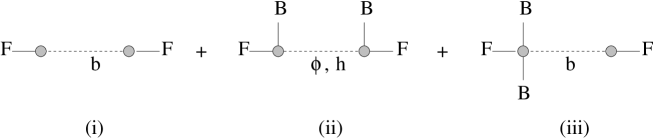
Figure 1: Two point amplitude upto quadratic order in $B$. (i) and (iii) are due to only $b$-field exchange, (ii) is due to graviton and dilaton exchange.

The propagators are the usual ones, rewriting them from eqns(34, 44,48),

$$<h_{ij}h_{i^{{}^{\prime}}j^{{}^{\prime}}}> = -2i\kappa^{2}\frac{[\eta_{ii^{{}^{\prime}}}\eta_{jj^{{}^{\prime}}}+\eta_{ij^{{}^{\prime}}}\eta_{i^{{}^{\prime}}j}-2/(D-2)\eta_{ij}\eta_{i^{{}^{\prime}}j^{{}^{\prime}}}]}{k_{\perp}^{2}+k_{\parallel}^{2}}$$ (68)

$$<\phi\phi> = -\frac{(D-2)i\kappa^{2}}{4}\frac{1}{k_{\perp}^{2}+k_{\parallel}^{2}}$$ (69)

$$<b_{ij}b_{i^{{}^{\prime}}j^{{}^{\prime}}}> = -\frac{2i\kappa^{2}}{(2\pi\alpha^{{}^{\prime}})^{2}}\frac{[\eta_{ii^{{}^{\prime}}}\eta_{jj^{{}^{\prime}}}-\eta_{ji^{{}^{\prime}}}\eta_{ij^{{}^{\prime}}}]}{k_{\perp}^{2}+k_{\parallel}^{2}}$$ (70)

With these, the contributions from the three modes to the two point function can be worked out. We are interested in the correction to the quadratic term in the effective action for the gauge field on the brane. This can be constructed with the vertices computed above and the propagators for the intermediate massless closed string states. This correction for the nonplanar diagram can be written as,

$$A_{2}(bb)=\int d^{p+1}\xi\int d^{p+1}\xi^{{}^{\prime}}b(\xi)b(\xi^{{}^{\prime}})V<\chi(\xi)\chi(\xi^{{}^{\prime}})>V$$ (71)

where,

$$<\chi(\xi)\chi(\xi^{{}^{\prime}})>=\int\frac{d^{D}k}{(2\pi)^{D}}<\chi(k_{\perp},k_{\parallel})\chi(-k_{\perp},-k_{\parallel})>e^{-ik_{\parallel}(\xi-\xi^{{}^{\prime}})}$$ (72)

We can rewrite eqn(71) in momentum space coordinates as,

$$A_{2}(bb) = {\cal V}_{p+1}\int\frac{d^{p+1}p}{(2\pi)^{p+1}}b(p)b(-p)\int\frac{d^{l}k_{\perp}}{(2\pi)^{l}}V<\chi(k_{\perp},-p)\chi(-k_{\perp},p)>V$$ (73)

$$= {\cal V}_{p+1}\int\frac{d^{p+1}p}{(2\pi)^{p+1}}b(p)b(-p)L_{2}(p,-p)$$

In the planar two point function, both the vertices are on the same end of the cylinder in the worldsheet computation. In the field theory this corresponds to putting both the vertices at the same position on the $D$-brane. In other words, in the expansion of the DBI action, we should be looking for $b^{2}\chi$ vertices on one end and a $\chi$ tadpole on the other. In this case, from the above calculation, $k_{\parallel}=0$. So the closed string propagator is just $1/k_{\perp}^{2}$, i.e. the propagator is not modified by the momentum of the gauge field on the brane. This is what we expect, as in the field theory on the brane, the loop integrals are not modified for the planar diagrams. Here we will only concentrate on the nonplanar sector.

As mentioned earlier, on the brane we will identify,

$$b_{kl}(p)\equiv\frac{g_{0}}{\sqrt{2\alpha^{{}^{\prime}}}}F_{kl}(p)=\frac{g_{0}}{\sqrt{2\alpha^{{}^{\prime}}}}p_{[k}A_{l]}(p)$$ (74)

For the graviton we have,

$$L_{2}(bhb) = \int\frac{d^{l}k_{\perp}}{(2\pi)^{l}}V_{h}^{ij,kl}<h_{ij}h_{i^{{}^{\prime}}j^{{}^{\prime}}}>V_{h}^{i^{{}^{\prime}}j^{{}^{\prime}},k^{{}^{\prime}}l^{{}^{\prime}}}$$ (75)

$$= -i\kappa^{2}\tau_{p}^{2}(2\pi\alpha^{{}^{\prime}})^{4}\int\frac{d^{l}k_{\perp}}{(2\pi)^{l}}\frac{2}{k_{\perp}^{2}+p^{2}}\times$$

$$\times \left[-B^{2ll^{{}^{\prime}}}\eta^{kk^{{}^{\prime}}}+B^{lk^{{}^{\prime}}}B^{l^{{}^{\prime}}k}+\left(\frac{p+1}{8}+\frac{p-1}{D-2}-\frac{(p+1)^{2}}{8(D-2)}-1\right)B^{lk}B^{l^{{}^{\prime}}k^{{}^{\prime}}}\right]$$

For the dilaton,

$$L_{2}(b\phi b) = \int\frac{d^{l}k_{\perp}}{(2\pi)^{l}}V_{\phi}^{kl}<\phi\phi>V_{\phi}^{k^{{}^{\prime}}l^{{}^{\prime}}}$$

$$= -i\kappa^{2}\tau_{p}^{2}(2\pi\alpha^{{}^{\prime}})^{4}\int\frac{d^{l}k_{\perp}}{(2\pi)^{l}}\frac{1}{k_{\perp}^{2}+p^{2}}\frac{(D-2)}{4}\left(\frac{1}{2}-\frac{p+1}{D-2}+\frac{4}{D-2}\right)^{2}B^{lk}B^{l^{{}^{\prime}}k^{{}^{\prime}}}$$

Adding the contributions from the graviton and the dilaton,

$$L_{2}(bhb+b\phi b) = -i\kappa^{2}\tau_{p}^{2}(2\pi\alpha^{{}^{\prime}})^{4}\int\frac{d^{l}k_{\perp}}{(2\pi)^{l}}\frac{1}{k_{\perp}^{2}+p^{2}}\times$$

$$\times \left[-2B^{2ll^{{}^{\prime}}}\eta^{kk^{{}^{\prime}}}+2B^{lk^{{}^{\prime}}}B^{l^{{}^{\prime}}k}+B^{lk}B^{l^{{}^{\prime}}k^{{}^{\prime}}}\left(\frac{D-2}{16}-1\right)\right]$$

Similarly for the $b$-field we have,

$$L_{2}(bbb) = \int\frac{d^{l}k_{\perp}}{(2\pi)^{l}}V_{b}^{ij,kl}<b_{ij}b_{i^{{}^{\prime}}j^{{}^{\prime}}}>V_{b}^{i^{{}^{\prime}}j^{{}^{\prime}},k^{{}^{\prime}}l^{{}^{\prime}}}$$

$$= -i\kappa^{2}\tau_{p}^{2}\int\frac{d^{l}k_{\perp}}{(2\pi)^{l}}\frac{1}{k_{\perp}^{2}+p^{2}}\times$$

$$\times [\frac{(2\pi\alpha^{{}^{\prime}})^{2}}{4}\{1-\frac{(2\pi\alpha^{{}^{\prime}})^{2}}{2}\mbox{Tr}(B^{2})\}(\eta^{ll^{{}^{\prime}}}\eta^{kk^{{}^{\prime}}}-\eta^{lk^{{}^{\prime}}}\eta^{kl^{{}^{\prime}}})$$

$$+ (2\pi\alpha^{{}^{\prime}})^{4}\{\frac{1}{2}B^{lk}B^{l^{{}^{\prime}}k^{{}^{\prime}}}+((B^{2})^{ll^{{}^{\prime}}}\eta^{kk^{{}^{\prime}}}-(B^{2})^{lk^{{}^{\prime}}}\eta^{kl^{{}^{\prime}}})$$

$$- \frac{1}{2}(B^{lk^{{}^{\prime}}}B^{l^{{}^{\prime}}k}-B^{ll^{{}^{\prime}}}B^{k^{{}^{\prime}}k})+(lk)\leftrightarrow(l^{{}^{\prime}}k^{{}^{\prime}})\}]$$

For the full two point function, there are cancellations between the eqn(4.1) and eqn(4.1). The final answer is,

$$L_{2} = -i\kappa^{2}\tau_{p}^{2}\int\frac{d^{l}k_{\perp}}{(2\pi)^{l}}\frac{1}{k_{\perp}^{2}+p^{2}}\times$$

$$\times [(2\pi\alpha^{{}^{\prime}})^{4}B^{lk}B^{l^{{}^{\prime}}k^{{}^{\prime}}}\frac{D-2}{32}+\frac{(2\pi\alpha^{{}^{\prime}})^{2}}{4}\{1-\frac{(2\pi\alpha^{{}^{\prime}})^{2}}{2}\mbox{Tr}(B^{2})\}(\eta^{ll^{{}^{\prime}}}\eta^{kk^{{}^{\prime}}}-\eta^{lk^{{}^{\prime}}}\eta^{kl^{{}^{\prime}}})$$

$$+ \frac{(2\pi\alpha^{{}^{\prime}})^{4}}{2}\{(B^{2})^{ll^{{}^{\prime}}}\eta^{kk^{{}^{\prime}}}-(B^{2})^{lk^{{}^{\prime}}}\eta^{kl^{{}^{\prime}}}\}+(lk)\leftrightarrow(l^{{}^{\prime}}k^{{}^{\prime}})]$$

The full two point effective action, can now be constructed by putting back $L_{2}$ in eqn(73) along with the identification eqn(74). To compare this with the closed string channel result with only massless exchanges, eqn(32) we must note the expansions of the following quantities to appropriate powers of $B$.

$$G^{ij} \sim \eta^{ij}+(2\pi\alpha^{{}^{\prime}})^{2}(B^{2})^{ij}+{\cal O}(B^{4})$$ (81)

$$\theta^{ij} \sim -(2\pi\alpha^{{}^{\prime}})^{2}B^{ij}+{\cal O}(B^{3})$$ (82)

$$\sqrt{\eta+(2\pi\alpha^{{}^{\prime}})B} \sim \left[1-\frac{(2\pi\alpha^{{}^{\prime}})^{2}}{4}\mbox{Tr}(B^{2})+{\cal O}(B^{4})\right]$$ (83)

With these expansions, we can see that eqn(32) equals the sum of massless contributions, in eqn(4.1).

4.2 Noncommutative case $(g=\epsilon\eta)$

We now turn to the Seiberg Witten limit, (5) which gives rise to noncommutative field theory on the brane. Here again we will be interested in writing out the two point function eqn(32) in the closed string channel as a sum of the massless closed string modes. Due to the scaling of the closed string metric, unlike the earlier case, we will now expand all results in powers of the scale parameter for closed string metric, $\epsilon$. We begin by expanding the DBI action,

$${\cal L}=\sqrt{(2\pi\alpha^{{}^{\prime}})e^{-(P+Q)\phi}(B+b)}\left[1+\frac{1}{(2\pi\alpha^{{}^{\prime}})e^{-Q\phi}(B+b)}\epsilon(\eta+h)\right]^{1/2}$$ (84)

For a matrix $M$, we have that following expansion,

$$\sqrt{1+M} = \mbox{exp}\left[\frac{1}{2}\mbox{Tr}\mbox{log}(1+M)\right]$$ (85)

$$= 1+\frac{1}{2}\mbox{Tr}(M-\frac{M^{2}}{2}+...)+\frac{1}{8}\left[\mbox{Tr}(M-\frac{M^{2}}{2}+...)\right]^{2}+...$$ (86)

For $M$ antisymmetric, terms containing $\mbox{Tr}(M)$ vanishes, hence to order $\epsilon^{2}$, we have,

$${\cal L} = \sqrt{(2\pi\alpha^{{}^{\prime}})e^{-(P+Q)\phi}(B+b)}\left[1-\frac{\epsilon^{2}}{4}\mbox{Tr}\left(\frac{1}{(2\pi\alpha^{{}^{\prime}})e^{-Q\phi}(B+b)}(\eta+h)\right)^{2}\right]$$ (87)

$$= \sqrt{(2\pi\alpha^{{}^{\prime}})e^{-(P+Q)\phi}(B+b)}\times$$

$$\times \left[1-\frac{\epsilon^{2}e^{2Q\phi}}{4(2\pi\alpha^{{}^{\prime}})^{2}}\mbox{Tr}\left[\frac{1}{B^{2}}\left(1-\frac{2}{B}b+3\frac{1}{B}b\frac{1}{B}b-...\right)(\eta+h)^{2}\right]\right]$$

Let us now first consider the ${\cal O}(1)$ term in $\epsilon$,

$${\cal L}\mid_{{\cal O}(1)}=\sqrt{(2\pi\alpha^{{}^{\prime}})e^{-(P+Q)\phi}(B+b)}$$ (88)

There is no graviton coupling at this order. The $\phi$ and $b$-field vertices from this are,

$$V_{\phi}^{1} = -\frac{1}{2}\sqrt{(2\pi\alpha^{{}^{\prime}})B}\left(\frac{1}{B}\right)^{lk}$$ (89)

$$V_{b}^{1} = \sqrt{(2\pi\alpha^{{}^{\prime}})B}\left[\frac{1}{4}\left(\frac{1}{B}\right)^{lk}\left(\frac{1}{B}\right)^{ji}-\frac{1}{2}\left(\frac{1}{B}\right)^{jk}\left(\frac{1}{B}\right)^{li}\right]$$ (90)

Now, let us consider the $\epsilon^{2}$ term. As in the earlier case let us define,

$$Y = \sqrt{(2\pi\alpha^{{}^{\prime}})e^{-(P+Q)\phi}(B+b)}$$ (91)

$$X = -\frac{\epsilon^{2}e^{2Q\phi}}{4(2\pi\alpha^{{}^{\prime}})^{2}}\mbox{Tr}\left[\frac{1}{B^{2}}\left(1-\frac{2}{B}b+3\frac{1}{B}b\frac{1}{B}b-...\right)(\eta+h)^{2}\right]$$ (92)

We are interested in the two point function only upto ${\cal O}(\epsilon^{2})$, hence we need not consider the graviton vertex. Also the $b$-field propagator has a $\epsilon^{2}$ factor (44). So, it is only necessary to compute the dilaton vertex at this order. Listing the required derivatives,

$$\frac{\delta Y}{\delta\phi}=-\sqrt{(2\pi\alpha^{{}^{\prime}})B}\mbox{\hskip 14.45377pt}\frac{\delta Y}{\delta b_{kl}}=\frac{1}{2}\sqrt{(2\pi\alpha^{{}^{\prime}})B}\left(\frac{1}{B}\right)^{lk}$$ (93)

$$\frac{\delta^{2}Y}{\delta b_{kl}\delta\phi}=V_{\phi}^{1}\mbox{\hskip 14.45377pt}\frac{\delta^{2}X}{\delta b_{kl}\delta\phi}=\frac{\epsilon^{2}4Q}{4(2\pi\alpha^{{}^{\prime}})^{2}}\left(\frac{1}{B^{3}}\right)^{lk}$$ (94)

$$\frac{\delta X}{\delta\phi}=-\frac{\epsilon^{2}2Q}{4(2\pi\alpha^{{}^{\prime}})^{2}}\mbox{Tr}\frac{1}{B^{2}}\mbox{\hskip 14.45377pt}\frac{\delta X}{\delta b_{kl}}=\frac{\epsilon^{2}2}{4(2\pi\alpha^{{}^{\prime}})^{2}}\left(\frac{1}{B^{3}}\right)^{lk}$$ (95)

After putting in all the appropriate derivatives, the vertices for the dilaton and the $b$-field upto ${\cal O}(\epsilon^{2})$ is given by,

$$V_{\phi} = \sqrt{(2\pi\alpha^{{}^{\prime}})B}\left[-\frac{1}{2}\left(\frac{1}{B}\right)^{lk}+\frac{\epsilon^{2}(4Q-2)}{4(2\pi\alpha^{{}^{\prime}})^{2}}\left(\left(\frac{1}{B^{3}}\right)^{lk}-\frac{1}{4}\mbox{Tr}\left(\frac{1}{B^{2}}\right)\left(\frac{1}{B}\right)^{lk}\right)\right]$$

$$V_{b} = V_{b}^{1}$$ (96)

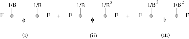
Figure 2: Two point amplitude upto ${\cal O}(\epsilon^{2})$. (i) and (ii) are due to dilaton exchange, (iii) is due to $b$-field exchange.

The situation in this case is similar to that of the earlier small $B$ expansion and is shown in Figure 2. The propagators in this limit, eqns(36,44),

$$<\phi\phi> = -\frac{(D-2)i\kappa^{2}}{4}\frac{1}{k_{\perp}^{2}+\epsilon^{-1}k_{\parallel}^{2}}$$ (97)

$$<b_{ij}b_{i^{{}^{\prime}}j^{{}^{\prime}}}> = -\frac{2i\kappa^{2}\epsilon^{2}}{(2\pi\alpha^{{}^{\prime}})^{2}}\frac{[\eta_{ii^{{}^{\prime}}}\eta_{jj^{{}^{\prime}}}-\eta_{ji^{{}^{\prime}}}\eta_{ij^{{}^{\prime}}}]}{k_{\perp}^{2}+\epsilon^{-1}k_{\parallel}^{2}}$$ (98)

With the vertices computed above and the propagator in this limit, the two point function for the dilaton is,

$$L_{2}(b\phi b) = -i\mbox{det}(2\pi\alpha^{{}^{\prime}}B)\kappa^{2}\tau_{p}^{2}\frac{(D-2)}{4}\int\frac{d^{l}k_{\perp}}{(2\pi)^{l}}\frac{1}{k_{\perp}^{2}+\epsilon^{-1}p^{2}}\times$$ (99)

$$\times \left[\frac{1}{8}\left(\frac{1}{B}\right)^{lk}\left(\frac{1}{B}\right)^{l^{{}^{\prime}}k^{{}^{\prime}}}-\frac{\epsilon^{2}(4Q-2)}{8(2\pi\alpha^{{}^{\prime}})^{2}}\left(\left(\frac{1}{B^{3}}\right)^{lk}-\frac{1}{4}\mbox{Tr}\left(\frac{1}{B^{2}}\right)\left(\frac{1}{B}\right)^{lk}\right)\left(\frac{1}{B}\right)^{l^{{}^{\prime}}k^{{}^{\prime}}}\right]$$

$$+ (lk)\leftrightarrow(l^{{}^{\prime}}k^{{}^{\prime}})$$

For the $b$-field,

$$L_{2}(bbb) = -i\mbox{det}(2\pi\alpha^{{}^{\prime}}B)\kappa^{2}\tau_{p}^{2}\frac{\epsilon^{2}}{(2\pi\alpha^{{}^{\prime}})^{2}}\int\frac{d^{l}k_{\perp}}{(2\pi)^{l}}\frac{2}{k_{\perp}^{2}+\epsilon^{-1}p^{2}}\times$$ (100)

$$\times [\left(\frac{1}{4}\left(\frac{1}{B^{3}}\right)^{lk}-\frac{1}{16}\mbox{Tr}\left(\frac{1}{B^{2}}\right)\left(\frac{1}{B}\right)^{lk}\right)\left(\frac{1}{B}\right)^{l^{{}^{\prime}}k^{{}^{\prime}}}$$

$$+ \frac{1}{8}\left(\frac{1}{B^{2}}\right)^{kk^{{}^{\prime}}}\left(\frac{1}{B^{2}}\right)^{ll^{{}^{\prime}}}-\frac{1}{8}\left(\frac{1}{B^{2}}\right)^{k^{{}^{\prime}}l}\left(\frac{1}{B^{2}}\right)^{lk^{{}^{\prime}}}$$

$$+ (lk)\leftrightarrow(l^{{}^{\prime}}k^{{}^{\prime}})]$$

The first two terms cancel with the $Q$-dependent terms of the dilaton, the resulting amplitude can now be written as,

$$L_{2} = -i\mbox{det}(2\pi\alpha^{{}^{\prime}}B)\kappa^{2}\tau_{p}^{2}\int\frac{d^{l}k_{\perp}}{(2\pi)^{l}}\frac{1}{k_{\perp}^{2}+\epsilon^{-1}p^{2}}[{\cal O}(1)+{\cal O}(\epsilon^{2})]$$ (101)

where,

$${\cal O}(1)=\left[\frac{(D-2)}{32}\left(\frac{1}{B}\right)^{lk}\left(\frac{1}{B}\right)^{l^{{}^{\prime}}k^{{}^{\prime}}}+(lk)\leftrightarrow(l^{{}^{\prime}}k^{{}^{\prime}})\right]$$ (102)

$${\cal O}(\epsilon^{2}) = \frac{\epsilon^{2}}{(2\pi\alpha^{{}^{\prime}})^{2}}\frac{(D-2)}{16}\left[\left[\left(\frac{1}{B^{3}}\right)^{lk}-\frac{1}{4}\mbox{Tr}\left(\frac{1}{B^{2}}\right)\left(\frac{1}{B}\right)^{lk}\right]\left(\frac{1}{B}\right)^{l^{{}^{\prime}}k^{{}^{\prime}}}\right]$$ (103)

$$+ \frac{\epsilon^{2}}{(2\pi\alpha^{{}^{\prime}})^{2}}\left[\frac{1}{4}\left(\frac{1}{B^{2}}\right)^{kk^{{}^{\prime}}}\left(\frac{1}{B^{2}}\right)^{ll^{{}^{\prime}}}-\frac{1}{4}\left(\frac{1}{B^{2}}\right)^{k^{{}^{\prime}}l}\left(\frac{1}{B^{2}}\right)^{lk^{{}^{\prime}}}\right]$$

$$+ (lk)\leftrightarrow(l^{{}^{\prime}}k^{{}^{\prime}})$$

We can now reconstruct the quadratic term in effective action, (73) following the earlier case. With the following expansions, it is easy to check that the sum of the massless contributions adds upto eqn(32).

$$G^{ij} \sim -\frac{\epsilon}{(2\pi\alpha^{{}^{\prime}})^{2}}\left(\frac{1}{B^{2}}\right)^{ij}+{\cal O}(\epsilon^{3})$$ (104)

$$\theta^{ij} \sim \left(\frac{1}{B}\right)^{ij}+\frac{\epsilon^{2}}{(2\pi\alpha^{{}^{\prime}})^{2}}\left(\frac{1}{B^{3}}\right)^{ij}$$ (105)

$$\sqrt{\epsilon\eta+(2\pi\alpha^{{}^{\prime}})B} \sim \sqrt{(2\pi\alpha^{{}^{\prime}})B}\left[1-\frac{\epsilon^{2}}{4(2\pi\alpha^{{}^{\prime}})^{2}}\mbox{Tr}\left(\frac{1}{B^{2}}\right)\right]$$ (106)

Note that, at the tree-level, to the linear order, $\hat{F}=F$, (9). At this quadratic order in the effective action there is no need for redefinition of $F$ to equate the result here with that of string theory result in eqn(32).

4.3 Noncommutative case ($G=\eta$)

In this part we finally consider the restriction of the open string metric, $G=\eta$. The lowest order solution for the closed string metric, $g$ in $\alpha^{{}^{\prime}}$ in this limit is,

$$g=-(2\pi\alpha^{{}^{\prime}})^{2}B^{2}+{\cal O}(\alpha^{{}^{\prime}4})$$ (107)

We will now consider expansions of the two point functions in powers of $\alpha^{{}^{\prime}}$. We begin again with the following DBI Lagrangian,

$${\cal L} = \sqrt{(2\pi\alpha^{{}^{\prime}})e^{-(P+Q)\phi}(B+b)}\left[1-\frac{1}{e^{-Q\phi}(B+b)}(2\pi\alpha^{{}^{\prime}})B^{2}(\eta+h)^{2}\right]^{1/2}$$ (108)

The calculation for the vertices is same as before, there is no graviton vertex to the leading orders. The dilaton and the $b$-field vertices are,

$$V_{\phi} = \sqrt{(2\pi\alpha^{{}^{\prime}})B}\left[-\frac{1}{2}\left(\frac{1}{B}\right)^{lk}+\frac{(2\pi\alpha^{{}^{\prime}})^{2}(4Q-2)}{4}\left(B^{lk}-\frac{1}{4}\mbox{Tr}(B^{2})\left(\frac{1}{B}\right)^{lk}\right)\right]$$

$$V_{b} = \sqrt{(2\pi\alpha^{{}^{\prime}})B}\left[\frac{1}{4}\left(\frac{1}{B}\right)^{lk}\left(\frac{1}{B}\right)^{ji}-\frac{1}{2}\left(\frac{1}{B}\right)^{jk}\left(\frac{1}{B}\right)^{li}\right]$$ (109)

The propagators for the dilaton and the $b$-field are modified as,

$$<\phi\phi> = -\frac{(D-2)i\kappa^{2}}{4}\frac{1}{k_{\perp}^{2}+\tilde{k_{\parallel}}^{2}/(2\pi\alpha^{{}^{\prime}})^{2}}$$ (110)

$$<b_{ij}b_{i^{{}^{\prime}}j^{{}^{\prime}}}> = -2i\kappa^{2}(2\pi\alpha^{{}^{\prime}})^{2}\frac{[B^{2}_{ii^{{}^{\prime}}}B^{2}_{jj^{{}^{\prime}}}-B^{2}_{ji^{{}^{\prime}}}B^{2}_{ij^{{}^{\prime}}}]}{k_{\perp}^{2}+\tilde{k_{\parallel}}^{2}/(2\pi\alpha^{{}^{\prime}})^{2}}$$ (111)

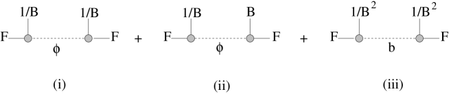
Figure 3: Two point amplitude upto ${\cal O}(\alpha^{{}^{\prime}2})$. (i) and (ii) are due to dilaton exchange, (iii) is due to $b$-field exchange.

With these vertices (shown in Figure 3) and the propagators from eqns(38,44), the two point functions are now given by,

$$L_{2}(b\phi b) = -i\mbox{det}(2\pi\alpha^{{}^{\prime}}B)\kappa^{2}\tau_{p}^{2}\frac{(D-2)}{4}\int\frac{d^{l}k_{\perp}}{(2\pi)^{l}}\frac{1}{k_{\perp}^{2}+\tilde{p}^{2}/(2\pi\alpha^{{}^{\prime}})^{2}}\times$$ (112)

$$\times \left[\frac{1}{8}\left(\frac{1}{B}\right)^{lk}\left(\frac{1}{B}\right)^{l^{{}^{\prime}}k^{{}^{\prime}}}-\frac{(2\pi\alpha^{{}^{\prime}})^{2}(4Q-2)}{8}\left(B^{lk}-\frac{1}{4}\mbox{Tr}(B^{2})\left(\frac{1}{B}\right)^{lk}\right)\left(\frac{1}{B}\right)^{l^{{}^{\prime}}k^{{}^{\prime}}}\right]$$

$$+ (lk)\leftrightarrow(l^{{}^{\prime}}k^{{}^{\prime}})$$

$$L_{2}(bbb) = -i\mbox{det}(2\pi\alpha^{{}^{\prime}}B)\kappa^{2}\tau_{p}^{2}(2\pi\alpha^{{}^{\prime}})^{2}\int\frac{d^{l}k_{\perp}}{(2\pi)^{l}}\frac{2}{k_{\perp}^{2}+\tilde{p}^{2}/(2\pi\alpha^{{}^{\prime}})^{2}}\times$$ (113)

$$\times \left[\left(\frac{1}{4}B^{lk}-\frac{1}{16}\mbox{Tr}(B^{2})\left(\frac{1}{B}\right)^{lk}\right)\left(\frac{1}{B}\right)^{l^{{}^{\prime}}k^{{}^{\prime}}}+\frac{1}{8}(\eta^{ll^{{}^{\prime}}}\eta^{kk^{{}^{\prime}}}-\eta^{kl^{{}^{\prime}}}\eta^{lk^{{}^{\prime}}})\right]$$

$$+ (lk)\leftrightarrow(l^{{}^{\prime}}k^{{}^{\prime}})$$

As before, the first term of the $b$ exchange cancels with the $Q$ dependent term of the dilaton exchange. The full two point answer is

$$L_{2}=-i\det(2\pi\alpha^{{}^{\prime}}B)\kappa^{2}\tau_{p}^{2}\int\frac{d^{l}k_{\perp}}{(2\pi)^{l}}\frac{1}{k_{\perp}^{2}+\tilde{p}^{2}(2\pi\alpha^{{}^{\prime}})^{2}}[{\cal O}(1)+{\cal O}(\alpha^{{}^{\prime}2})]$$ (114)

$${\cal O}(1)=\left[\frac{(D-2)}{32}\left(\frac{1}{B}\right)^{lk}\left(\frac{1}{B}\right)^{l^{{}^{\prime}}k^{{}^{\prime}}}+(lk)\leftrightarrow(l^{{}^{\prime}}k^{{}^{\prime}})\right]$$ (115)

$${\cal O}(\alpha^{{}^{\prime}2}) = (2\pi\alpha^{{}^{\prime}})^{2}\frac{(D-2)}{16}\left[\left[B^{lk}-\frac{1}{4}\mbox{Tr}(B^{2})\left(\frac{1}{B}\right)^{lk}\right]\left(\frac{1}{B}\right)^{l^{{}^{\prime}}k^{{}^{\prime}}}\right]$$ (116)

$$+ (2\pi\alpha^{{}^{\prime}})^{2}\left[\frac{1}{4}\left(\eta^{ll^{{}^{\prime}}}\eta^{kk^{{}^{\prime}}}-\eta^{kl^{{}^{\prime}}}\eta^{lk^{{}^{\prime}}}\right)\right]$$

$$+ (lk)\leftrightarrow(l^{{}^{\prime}}k^{{}^{\prime}})$$

We will need the following expansions in this limit, to expand the closed string channel result upto this order. We have already set,

$$G^{ij} = \eta^{ij}$$ (117)

and with the solution for $g$, eqn(107) to the lowest order in $\alpha^{{}^{\prime}}$,

$$\theta^{ij} \sim \left(\frac{1}{B}\right)^{ij}+(2\pi\alpha^{{}^{\prime}})^{2}B^{ij}$$ (118)

$$\sqrt{g+(2\pi\alpha^{{}^{\prime}})B} \sim \sqrt{(2\pi\alpha^{{}^{\prime}})B}\left[1-\frac{(2\pi\alpha^{{}^{\prime}})^{2}}{4}\mbox{Tr}(B^{2})\right]$$ (119)

As in the earlier cases, the massless contributions computed here, eqn(114) adds upto eqn(32). Note that the situation here is similar to that of the earlier case in section(4.2). As $\alpha^{{}^{\prime}}\sim\sqrt{\epsilon}$, the closed string metric in both the cases goes to zero as $g\sim\epsilon$. However the difference being that the two point amplitude differ by powers of $B$ in both the cases, due to the relative power of $B^{2}$ in $g$ in this case. Here too, the SW map between the usual and the noncommutative field strength eqn(9), remains the same. The differences in the powers of $B$ in the two point amplitudes, eqn(101) and eqn(114) are absorbed in $G$, $\theta$ and $\sqrt{g+(2\pi\alpha^{{}^{\prime}})B}$ in the two cases. We can work with any of the forms of the closed string metric $g$, the important point being that $g$ should go to zero as $\epsilon$ which gives the noncommutative gauge theory on the brane.

5 Discussions

Figure 4: Noncommutative field theory and closed string channel limits

Figure 4 sums up the various limits involved in the problem addressed in this paper. Noncommutative field theory arises in the Seiberg Witten limit. In the open string one loop amplitude, the $t\rightarrow\infty$ region of the moduli space of the cylinder corresponds to the IR regime with only contributions to the amplitude coming from the massless open string modes propagating in the loop. As a result we get a one loop two point function in noncommutative field theory. The other limit $t\rightarrow 0$, corresponds to the UV region of the open string loop. The one loop open string in this limit factorises in the closed string channel. The contributions in this region come from the massless tree level exchanges of the closed string modes. We have discussed in section 3. that the divergences arising from the two ends are related to each other (upto some overall normalisation). This relation could not be made exact in the setup considered here due to the presence of tachyons, which act as additional sources for divergences. We have shown that the tensor structure for the noncommutative field theory (12) two point amplitude can be recovered by considering massless and tachyonic exchanges of closed strings in the presence of background constant $B$-field. For the coefficient to match with the gauge theory result, in the bosonic string case, that we have studied, the full tower of the closed string states are required. We expect that an exact correspondence between the UV behavior of the noncommutative gauge theory and massless closed string exchanges may be made in some compactified superstring theory, where the gauge theory is four dimensional and the closed strings move in exactly two extra transverse directions [22]. This would cure the problem of tachyons as well as lead to the desired forms of propagators in the closed string channel. Keeping this in mind we have studied massless closed string exchanges in the background $B$-field. Apart from this it is an interesting problem by itself. The full two point amplitude in the presence of background $B$-field must be of the form (32). We have reconstructed this from the sum of massless (graviton, dilaton and $b$-field) exchanges with the vertices computed from the DBI action, by considering expansions of the amplitude in three different cases. This exercise has helped in isolating the contributions from each of the massless closed string modes separately. On the broader side this is one of the steps in the chain of limits in Figure 4. We can view these results in the light of open/closed string duality, as quantities in the boundary noncommutative gauge theory are being recovered from the bulk theory of closed strings. In the usual case there are infinities on both sides, manifested as UV in one and IR in the other. The $B$-field in the SW limit acts as a background where at least a subsector (nonplanar) of the gauge theory is regularised. This is the sector that has been the subject in this paper. It would be interesting to find a limit where only the nonplanar sector of the noncommutative gauge theory survives.

References

[1]
M. R. Douglas and C. M. Hull,
“D-branes and the noncommutative torus,”
JHEP 9802 (1998) 008
[arXiv:hep-th/9711165].
[2]
V. Schomerus,
“D-branes and deformation quantization,”
JHEP 9906 (1999) 030
[arXiv:hep-th/9903205].
[3]
C. S. Chu and P. M. Ho,
“Noncommutative open string and D-brane,”
Nucl. Phys. B 550 (1999) 151
[arXiv:hep-th/9812219].
[4]
N. Seiberg and E. Witten,
“String theory and noncommutative geometry,”
JHEP 9909 (1999) 032
[arXiv:hep-th/9908142].
[5]
M. R. Douglas and N. A. Nekrasov,