Phase shift approach in the case of a magnetic
flux tube

Abstract

In Refs. [2, 4] two different approaches have been developed for the numerical computation of the effective energy in the presence of a magnetic flux tube, by using the phase shift method. However, the opinion has been expressed that these two variations of the phase shift method are not equivalent. In this paper we aim to solve this ambiguity by comparing these two different approaches and showing that they give identical numerical results, within the numerical accuracy of the method.

1 Introduction

The numerical computation of the fermion-induced effective energy , in the presence of inhomogeneous magnetic fields of the form of a flux tube, is a topic that has attract the attention of several authors, see Refs. [1, 2, 3, 4].

In Refs. [2, 4] two different approaches have been developed for the numerical computation of the quantum energy in the presence of a magnetic flux tube, by using the phase shift method. The question that arises is whether these two different approaches are equivalent or not. In this paper we show, mainly by performing numerical computations, the equivalence of these two different approaches. In this way we give a detailed answer to the objections in Ref. [4], according to which the integral we used for the numerical computation of the 3+1 effective energy is not properly renormalized, and as a result it does not give the correct values for the effective energy.

For this reason, in section 2 we present in a detailed way the renormalization procedure we followed in Ref. [2], and we emphasize that exactly the same method has been used by other authors, and especially in Ref. [6]. In section 3 we present our numerical results for the integrand of Eq. (12) for the quantum energy, in the case of the Gaussian magnetic flux tube (of Eq. (16) below). These results indicate a highly convergent behavior for the integral of Eq. (12). In section 4, we compare our results (Fig. 2 in this work), for the quantum energy in the presence of the Gaussian flux tube, with the correspondent results of Ref. [4] (Fig. 4 in Ref. [4]), and we obtain that they are identical, within the numerical error of the method. Finally, in section 5 we compare the two methods more carefully by using a different way (comparing with the vacuum polarization diagram) and we find again that they should be equivalent.

2 Renormalization of the quantum energy

In this section we explain in detail the renormalization procedure we used in Ref. [2].

The quantum part of the fermion-induced effective energy in the presence of a magnetic field is given by the equation:

$$E_{Q}=-\frac{1}{2iT}Tr\ln(\not\!\!D^{2}+m^{2}_{f})$$ (1)

where $\not\!\!\!D=\gamma^{\mu}D_{\mu}$ $(\mu=0,1,2,3)$ and $D_{\mu}=\partial_{\mu}-ieA_{\mu}$. The gamma matrices satisfy the relationship $\{\gamma^{\mu},\gamma^{\nu}\}=2g^{\mu\nu}$, and $T$ is the total length of time.

We have shown in Ref. [2] that the $2+1$ quantum energy for a magnetic field of the form of a flux tube is given by the equation

$$E_{Q(2+1)}=\frac{1}{2\pi}\int_{0}^{+\infty}dk\frac{k}{\sqrt{k^{2}+m^{2}_{f}}}(\Delta(k)-c)$$ (2)

where $c=\lim_{k\rightarrow+\infty}\Delta(k)$. Our numerical study, in Ref. [2], shows that $c=-\pi\phi^{2}$ ($\phi=e\Phi/2\pi$). This means that $c$ is independent of the special form of the magnetic field we examine and depends only on the total magnetic flux of the field $\Phi$. We also note that $c$ arises from an integration by parts (for details see Ref. [2]) and it is not a quantity we subtract and add back in order to make the above integral convergent.

The function $\Delta(k)$ was defined in Ref. [2] as the symmetrical sum over l:

$$\Delta(k)=\lim_{L\rightarrow+\infty}\sum_{s,l=-L}^{L}\delta_{l,s}(k)$$ (3)

where $\delta_{l,s}(k)$ is the phase shift which corresponds to $l^{th}$ partial wave with momentum $k$ and spin $s$.

It is well known that there are no divergencies in 2+1 dimensional QED. From this point of view we expect the above integral of Eq. (2) to be convergent. In addition, our numerical results, for the integrand of Eq. (2), confirm with very good accuracy this expected convergent behavior, see Fig. 1 in Ref. [2], or Fig. 1 and Fig. 3 below in this paper. The calculation of the phase shifts have been performed by solving an ordinary differential equation. For details see Refs. [2, 9].

The corresponding $3+1$ dimensional result is obtained by the $2+1$ quantum energy if we replace $m_{f}^{2}$ by $k_{3}^{2}+m_{f}^{2}$ in (2) and integrate over the $k_{3}$ momentum [6]. An overall factor of $2$ (from the Dirac trace) must also be included.

$$E_{Q(3+1)}=\frac{1}{\pi}\int_{0}^{+\infty}dk\int_{-\Lambda/2}^{\Lambda/2}\frac{dk_{3}}{2\pi/L_{z}}\frac{k}{\sqrt{k^{2}+k_{3}^{2}+m^{2}_{f}}}(\Delta(k)-c)$$ (4)

As the integral over $k_{3}$ is divergent we have introduced a regularization parameter $\Lambda/2$. Now, if we integrate over $k_{3}$ we obtain the unrenormalized quantum energy per unit length $L_{z}$ ($L_{z}$ is the length of the space box towards $z$ direction) equal to

$$E_{Q(3+1)}=-\frac{1}{2\pi^{2}}\int_{0}^{+\infty}dkk\ln\left(\frac{k^{2}+m^{2}_{f}}{m_{f}^{2}}\right)(\Delta(k)-c)+\frac{1}{2\pi^{2}}\ln(\frac{\Lambda^{2}}{m_{f}^{2}})\int_{0}^{+\infty}dkk(\Delta(k)-c)$$ (5)

In the weak field limit $eB<<m_{f}^{2}$, or for large $m_{f}$, the above expression for the effective energy must tend to the first diagram (vacuum polarization diagram) of the perturbative expansion of the effective energy:

$$E_{Q(3+1)}^{(2)}= - \frac{1}{8\pi^{3}}\int_{0}^{1}dxx(1-x)\int_{0}^{+\infty}dqq|\widetilde{B}(q)|^{2}\ln(\frac{m_{f}^{2}+q^{2}x(1-x)}{m_{f}^{2}})$$ (6)

$$+ \frac{1}{24\pi^{2}}\ln(\frac{\Lambda^{2}}{m_{f}^{2}})\int d^{2}\vec{x}B^{2}(\vec{x})$$

where $\widetilde{B}(q)=\int d^{2}\vec{x}\>e^{-i\vec{q}\>\cdot\vec{x}}B(\vec{x})$, and we have assumed the rescaling $B\rightarrow eB$.

Note that the vacuum polarization diagram for the 3+1 dimensional case (see Eq. (6) above) can be obtained from 2+1 dimensional result

$$E^{(2)}_{Q(2+1)}=\frac{1}{16\pi^{3}}\int d^{2}\vec{q}\;|\widetilde{B}(\vec{q})|^{2}\int_{0}^{1}dx\frac{x(1-x)}{\sqrt{m_{f}^{2}+x(1-x)\vec{q}\>^{2}}}$$ (7)

if we set $m_{f}^{2}\rightarrow k_{3}^{2}+m_{f}^{2}$ and integrate over the $k_{3}$ momentum (an overall factor of $2$ must also be included).

By comparing Eqs. (5) and (6) in the weak field limit we obtain that

$$\int_{0}^{+\infty}dkk(\Delta(k)-c)=\frac{1}{12}\int d^{2}\vec{x}B^{2}(\vec{x})$$ (8)

Note that we have confirmed the above equation numerically by performing numerical computation for several magnetic fields of the form of a flux tube.

Now Eq. (5), for the unrenormalized quantum energy, can be written as

$$E_{Q(3+1)} = \frac{1}{2\pi^{2}}\int_{0}^{+\infty}dkk\ln\left(\frac{k^{2}+m^{2}_{f}}{m_{f}^{2}}\right)(\Delta(k)-c)$$ (9)

$$+ \frac{1}{24\pi^{2}}\ln(\frac{\Lambda^{2}}{m_{f}^{2}})\int d^{2}\vec{x}B^{2}(\vec{x})$$

The logarithmically divergent term can be incorporated in the classical energy, as is shown below

$$E_{eff} = E_{class}+E_{Q}$$ (10)

$$= \frac{1}{2}\left(\frac{1}{e^{2}}+\frac{1}{12\pi^{2}}\ln(\frac{\Lambda^{2}}{m_{f}^{2}})\right)\int d^{2}\vec{x}B^{2}(\vec{x})$$

$$+ \frac{1}{2\pi^{2}}\int_{0}^{+\infty}dkk\ln\left(\frac{k^{2}+m^{2}_{f}}{m_{f}^{2}}\right)(\Delta(k)-c)$$

In this way the logarithmically divergent part corresponds to a charge renormalization according to the equation

$$\frac{1}{e^{2}_{R}}=\frac{1}{e^{2}}+\frac{1}{12\pi^{2}}\ln(\frac{\Lambda^{2}}{m_{f}^{2}})$$ (11)

and thus the renormalized quantum energy is

$$E_{Q(3+1)}^{(ren)}=-\frac{1}{2\pi^{2}}\int_{0}^{+\infty}dkk\ln\left(\frac{k^{2}+m^{2}_{f}}{m_{f}^{2}}\right)(\Delta(k)-c)$$ (12)

The above presented renormalization procedure corresponds to the on-shell renormalization condition $\Pi(0)=0$ (for more details see Ref. [8]).

Now, as the divergent part has been removed, the integral of Eq. (12), for the renormalized quantum energy, is expected to be convergent. In the next section, we will indeed see that our numerical results indicate a highly convergent behavior for this integral.

Note that exactly the same renormalization procedure has been used by the authors of Ref. [6]. Particularly, in Ref. [6] the analytical result for the 2+1 quantum energy for a special form of an inhomogeneous magnetic field is taken for granted from their previous work of Ref [10]. Then the replacement $m_{f}^{2}\rightarrow k_{3}^{2}+m_{f}^{2}$ is performed, and the 3+1 dimensional result is obtained by integrating out the $k_{3}$ momentum. As we did in this paper, a cut-off $\Lambda/2$ is used in Ref. [6] for the regularization of the integral over $k_{3}$, and the same logarithmically divergent term arises. This term can be removed as it corresponds to a charge renormalization. In Ref. [6] we see that the remaining part, which corresponds to the regularized quantum energy, is an analytical formula with no divergencies.

3 Convergence of the integral of Eq. (12)

For the numerical computations we have chosen the Gaussian magnetic field

$$B_{G}(r)=\frac{2\phi}{d^{2}}\>\exp(-\frac{r^{2}}{d^{2}})$$ (13)

where $d$ is the spatial size of the magnetic flux tube, $\phi=e\Phi/2\pi$, and $\Phi$ is the total magnetic flux of the field.

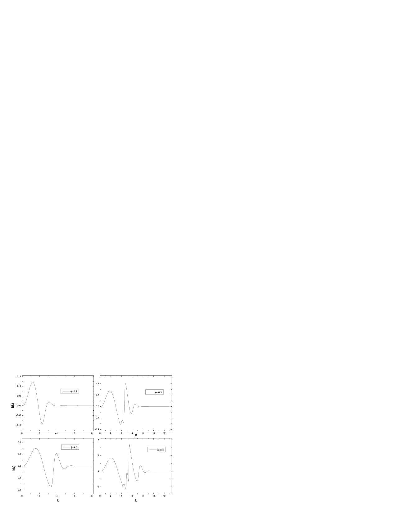
Figure 1: The integrand $I(k)$ as a function of $k$ for $\phi=2.5,4.5,6.5,8.5$ and $m_{f}=1$, in the case of the Gaussian magnetic field of Eq. (16).

In Fig. 1 we have plotted the integrand of Eq. (12)

$$I(k)=\frac{1}{2\pi^{2}}k\ln\left(\frac{k^{2}+m^{2}_{f}}{m_{f}^{2}}\right)(\Delta(k)-c)$$ (14)

as a function of $k$ for $\phi=2.5,4.5,6.5,8.5$, $d=1$ and $m_{f}=1$.

We see that our numerical results in Fig. 1 indicate a highly convergent behavior for the integral of Eq. (12), as the integrand $I(k)$ becomes zero for sufficiently large values of $k$.

4 Comparing with the results of Ref. [4]

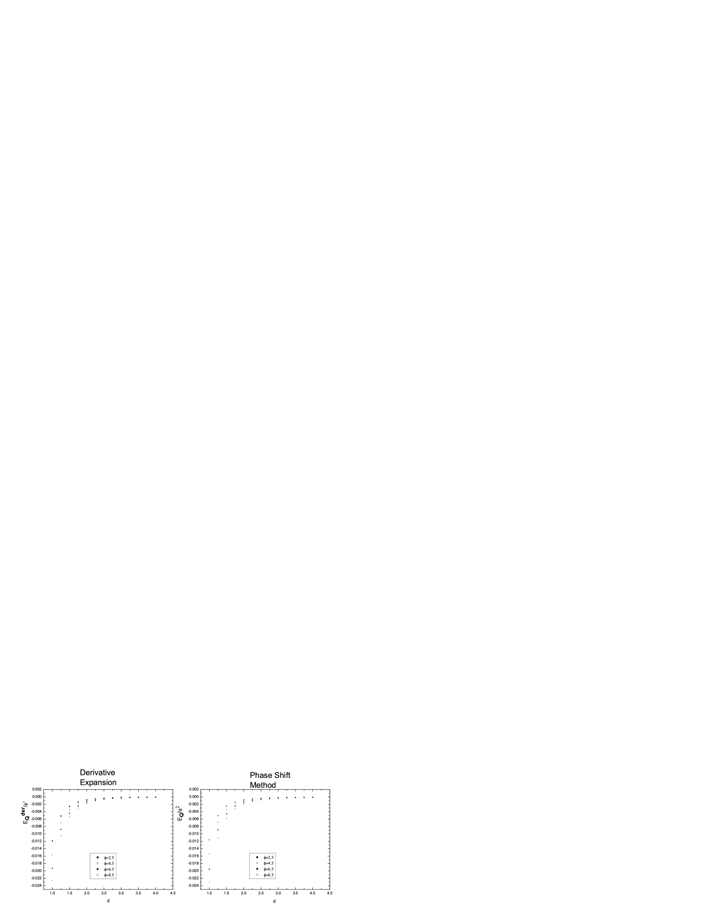
Figure 2: Derivative Expansion versus Phase Shift Method for the Gaussian magnetic flux tube, for $\phi=2.5,4.5,6.5,8.5$ and $m_{f}=1$.

As the convergence of the integral of Eq. (12) is not sufficient to show that our numerical results for the quantum energy are the same with those of the phase shift approach of Ref. [4], we should perform a comparison of the numerical results of these two different approaches.

For this we have plotted $E^{(ren)}_{Q(3+1)}/\phi^{2}$ as a function of $d$ for $\phi=2.5,4.5,6.5,8.5$ and $m_{f}=1$, in the right-hand panel of Fig. 2. We see that our results in this figure are identical (within the numerical accuracy of the method) with the corresponding results of Ref. [4] (see the right-hand panel of Fig. (4) in Ref. [4]).

Also, it is worth to compare the results of the phase shift method with the derivative expansion, which is the standard approximative tool in the case of smooth inhomogeneous magnetic fields (see for example Ref. [5]). In Fig. 2 we see that our results are in a very good agreement with the corresponding results of the derivative expansion in the homogeneous limit $1/\sqrt{B_{m}}<<d$, as is expected, where $B_{m}=2\phi/d^{2}$ .

5 Phase shift approach and vacuum polarization diagram

Figure 3: $\Delta(k)-c$ and $\overline{\Delta}(k)=\Delta(k)-\phi^{2}\Delta^{(2)}(k)$ as a function of k for $\phi=6.5$, $m_{f}=1$ and d=1, where $c=-\pi\phi^{2}$.

Figure 4: $\Delta^{(2)}(k)+\pi$ and $I_{2}(k)$ as a function of k for d=1 and $m_{f}=1$. We see that $\Delta^{(2)}(k)\rightarrow-\pi$ as $k\rightarrow+\infty$.

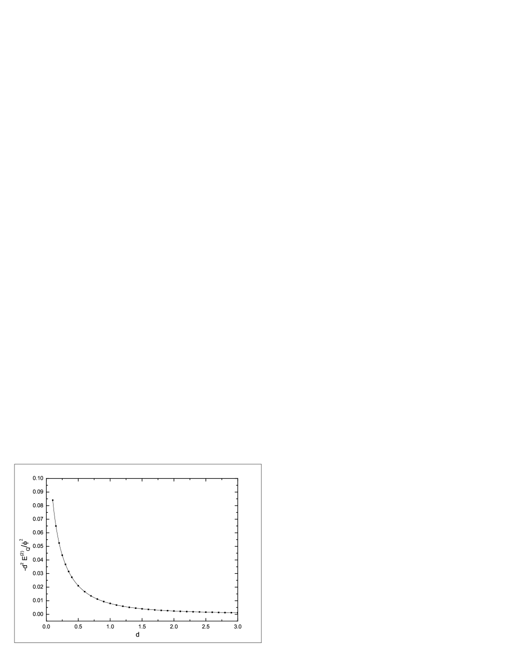
Figure 5: We have plotted the first and the second member of Eq. (21), multiplied by $-d^{2}/\phi^{2}$, as a function of $d$ for $m_{f}=1$. The continuous line corresponds to the vacuum polarization diagram, and the discrete points to the phase shift integral. According to this figure, Eq. (21) is valid.

In Ref. [4] the renormalized quantum energy $E^{\prime}_{Q(3+1)}$ is computed as a sum of two terms

$$E^{\prime}_{Q(3+1)}=E_{ph(3+1)}+E^{(2)}_{Q(3+1)}$$ (15)

where the first term corresponds to the contribution of the phase shifts

$$E_{ph(3+1)}=-\frac{1}{2\pi^{2}}\int_{0}^{+\infty}dkk\ln\left(\frac{k^{2}+m^{2}_{f}}{m_{f}^{2}}\right)\overline{\Delta}(k)$$ (16)

and the second term $E^{(2)}_{Q(3+1)}$ is the renormalized quantum energy which corresponds to the vacuum polarization diagram (see Eq. (8)).

The function $\overline{\Delta}(k)$ is defined as

$$\overline{\Delta}(k)=\lim_{L\rightarrow+\infty}\sum_{s,l=-L}^{L}\overline{\delta}_{l,s}(k)$$ (17)

where

$$\overline{\delta}_{l,s}(k)={\delta}_{l,s}(k)-\phi{\delta}_{l,s}^{(1)}(k)-\phi^{2}{\delta}_{l,s}^{(2)}(k)$$ (18)

and ${\delta}_{l,s}^{(1)}(k)$, ${\delta}_{l,s}^{(2)}(k)$ are the coefficients of $\phi$ and $\phi^{2}$ which arise if we expand the phase shift ${\delta}_{l,s}(k)$ in powers of $\phi$.

We emphasize that ${\delta}_{l,s}^{(1)}(k)$ and ${\delta}_{l,s}^{(2)}(k)$ are not the first and second Born approximations, as the Born expansion is an expansion in powers of the potential $v_{l,s}(r)$ of the corresponding scattering problem, and this potential includes both terms of $\phi$ and $\phi^{2}$.

From Eqs. (17) and (18) we obtain

$$\overline{\Delta}(k)=\Delta(k)-\phi^{2}\Delta^{(2)}(k)$$ (19)

as we can prove, from the integral formula for the first Born approximation, that $\Delta^{(1)}(k)=0$.

Note that the functions $\Delta^{(1)}(k)$ and $\Delta^{(2)}(k)$ are defined as:

$$\Delta^{(1)}(k)=\lim_{L\rightarrow+\infty}\sum_{s,l=-L}^{L}\delta^{(1)}_{l,s}(k)\;,\qquad\Delta^{(2)}(k)=\lim_{L\rightarrow+\infty}\sum_{s,l=-L}^{L}\delta^{(2)}_{l,s}(k)$$

In Fig. 3 we have plotted $\Delta(k)-c=\Delta(k)+\pi\phi^{2}$ and $\overline{\Delta}(k)=\Delta(k)-\phi^{2}\Delta^{(2)}(k)$ as a function of k for $\phi=6.5$, $m_{f}=1$ and d=1. We see that very shortly ($k>2$) these two functions become identical. The main reason is that the function $\Delta^{(2)}(k)$ tents rapidly to $-\pi$, as we see in the left-hand panel of Fig. 4.

The immediate consequence of the above discussion is that the integrals of Eqs. (12) and (16) have exactly the same convergent properties. Thus, Eq. (16), which was used for the computation of the quantum energy in Ref. [4], has no additional advantage against Eq. (12) which we used in our work of Ref. [2]. On the other hand, if we use Eq. (12) for the quantum energy, it is not necessary to compute additional quantities like the phase shifts ${\delta}_{l,s}^{(2)}(k)$ and the vacuum polarization diagram.

In addition, in the previous section we see that the results of these two variations of the phase shift method are in a very good agreement, however in this section we will go over this topic more carefully.

If we demand the results of two methods to be equal ($E_{Q(3+1)}=E^{\prime}_{Q(3+1)}$ see Eqs (12) and (15)), from Eqs. (6), (12), (15), (16) we obtain

$$- \frac{1}{2\pi^{2}}\int_{0}^{+\infty}dkk\ln\left(\frac{k^{2}+m^{2}_{f}}{m_{f}^{2}}\right)\left(\Delta(k)-c\right)=-\frac{1}{2\pi^{2}}\int_{0}^{+\infty}dkk\ln\left(\frac{k^{2}+m^{2}_{f}}{m_{f}^{2}}\right)\overline{\Delta}(k)$$ (20)

$$- \frac{1}{8\pi^{3}}\int_{0}^{1}dxx(1-x)\int_{0}^{+\infty}dqq|\widetilde{B}(q)|^{2}\ln(\frac{m_{f}^{2}+q^{2}x(1-x)}{m_{f}^{2}})$$

or, if we use Eq. (19), we obtain the equivalent equation

$$- \phi^{2}\frac{1}{2\pi^{2}}\int_{0}^{+\infty}dkk\ln\left(\frac{k^{2}+m^{2}_{f}}{m_{f}^{2}}\right)\left(\Delta^{(2)}(k)+\pi\right)$$ (21)

$$= -\frac{1}{8\pi^{3}}\int_{0}^{1}dxx(1-x)\int_{0}^{+\infty}dqq|\widetilde{B}(q)|^{2}\ln(\frac{m_{f}^{2}+q^{2}x(1-x)}{m_{f}^{2}})$$

In Fig. 5 we have plotted the first and the second member of Eq. (21), multiplied by $-d^{2}/\phi^{2}$, as a function of $d$ for $m_{f}=1$. The continuous line corresponds to the vacuum polarization diagram, and the discrete points to the phase shift integral of the first member of Eq. (21). Thus, from Fig. 5, it is seen that the first and second member of Eq. (21) are equal (the deviations between the numerical values of the first and second member of Eq. (21) are of the order of 0.1 per cent). As a result the two alternative approaches, for the quantum energy in the presence of a flux tube, are equivalent.

In addition, if take into account the above results, we can compute the difference $|E_{Q(3+1)}-E^{\prime}_{Q(3+1)}|$, where $E_{Q(3+1)}$ and $E^{\prime}_{Q(3+1)}$ are the renormalized quantum energies which correspond to the two variations of the phase shift method, see also Eq. (12) and (16). We see that $|E_{Q(3+1)}-E^{\prime}_{Q(3+1)}|/E_{Q(3+1)}\approx 0.001$, which is of the order of the accuracy of the numerical computations, and as a result the numerical values for $E_{Q(3+1)}$ and $E^{\prime}_{Q(3+1)}$ are identical.

Note that, according to the above discussion, the first member of Eq. (21) can be viewed as the phase shift representation of the vacuum polarization diagram, or we can write

$$E_{Q(3+1)}^{(2)}=-\phi^{2}\frac{1}{2\pi^{2}}\int_{0}^{+\infty}dkk\ln\left(\frac{k^{2}+m^{2}_{f}}{m_{f}^{2}}\right)\left(\Delta^{(2)}(k)+\pi\right)$$ (22)

In order to study the convergent properties of the above integral, we have plotted, in the right-hand panel of Fig. 4, the integrand of Eq. (22)

$$I_{2}(k)=\frac{1}{2\pi^{2}}k\ln\left(\frac{k^{2}+m^{2}_{f}}{m_{f}^{2}}\right)\left(\Delta^{(2)}(k)+\pi\right)$$ (23)

for $d=1$ and $m_{f}=1$. We see that that Fig. 4 indicates a highly convergent behavior for the integral of Eq. (22).

6 Conclusions

In this paper we compared the results of the two different variations of the phase shift method, of Refs. [2, 4], for the numerical computation of the quantum energy in the presence of a magnetic flux tube. In section 3 and 4 we show, mainly by performing numerical computations, that these two alternative approaches give identical values for the quantum energy ($|E_{Q(3+1)}-E^{\prime}_{Q(3+1)}|/E_{Q(3+1)}\approx 0.001$, see section 4), and as a result they are equivalent.

In addition, in section 4 we show that in order to make the integral over k, of Eq. (12), convergent, it is not necessary to subtract the $\phi$ and $\phi^{2}$ parts of the phase shift $\delta_{l,s}(k)$ (see Eq. 18) and to add them back in their Feynman diagrammatic form, as is done in Ref. [4]. This immediate convergence of the integral of Eq. (12) is a consequence of the translation invariance along the $x_{3}$ axis. However, in the case of problems, e.g. with spherical symmetry, where the translation invariance is violated, the subtraction of the asymptotic part of the phase shift sum $\sum_{s,l=0}^{+\infty}\delta_{l,s}(k)$ (or the subtraction of the first and second Born approximation), in order to make the integral over $k$ convergent, is unavoidable (see Refs. [9, 11]).

It is worth to mention, that for the computation of the quantum energy in the presence of a magnetic flux tube, two other alternative methods have been developed: $a)$ the Jost function method in Ref. [1] and $b)$ the method of the worldline numerics in Ref. [3]. Note, that in Ref. [2] we have compared our results to the Jost function method, in the case of a discontinuous magnetic field which is constant inside a cylinder of radius $d$, and zero outside it. From Fig. 4 in Ref. [2] and the Fig. 3 in Ref. [1] we see a very good agreement between the phase shift and Jost function method.

Finally, it would be interesting if the two alternative approaches ( the Jost function and the worldline method) could give a figure like that of the right-hand panel of Fig. 2 of this work, for a smooth realistic magnetic field like the Gaussian magnetic flux tube.

7 Acknowledgements

I am grateful to Professors G. Tiktopoulos and K. Farakos for important discussions. The work of P.P was supported by the ”Pythagoras” project of the Greek Ministry of Education.

References

- [1] M. Bordag and K. Kirsten, Phys. Rev. D 60, 105019 (1999).
- [2] P. Pasipoularides, Phys. Rev. D 64, 105011 (2001).
- [3] K. Langfeld, L. Moyaerts, H. Gies, Nucl.Phys., B646:158-180 (2002).
- [4] N. Graham, V. Khemani, M. Quandt, O. Schroder, H. Weigel. Nucl. Phys. B707:233-277 (2005).
- [5] V.P. Gusynin and I.A. Shovkovy, J. Math. Phys. 40, 5406 (1999).
- [6] G. Dunne and T. Hall, Phys. Lett. B 419, 322 (1998).
- [7] Y. Aharonov and A. Casher, Phys. Rev. A 19, 2461 (1979).
- [8] M. E. Peskin and D. V. Schroeder, An Introduction to Quantum Field Theory, Addison-Wesley Pubplishing Company.
- [9] E. Farhy, N. Graham, P. Haagensen and R.L. Jaffe, Phys.Lett. 427B, 334 (1998).
- [10] D. Cangemi, E. D’Hoker and G. Dunne, Phys. Rev. D 52, 3163 (1995).
- [11] B. Moussallam, Phys. Rev. D 40, 3430 (1989).