We further investigate the $NS$5 ring background using the tachyon map. Mapping the radion fields to the rolling tachyon helps to explain the motion of a probe $Dp$-brane in this background. It turns out that the radion field becomes tachyonic when the brane is confined to one dimensional motion inside the ring. We find explicit solutions for the geometrical tachyon field that describe stable kink solutions which are similar to those of the open string tachyon. Interestingly in the case of the geometric tachyon, the dynamics is controlled by a cosine potential. In addition, we couple a constant electric field to the probe-brane, but find that the only stable kink solutions occur when there is zero electric field or a critical field value. We also investigate the behaviour of Non-BPS branes in this background, and find that the end state of any probe brane is that of tachyonic matter ’trapped’ around the interior of the ring. We conclude by considering compactification of the ring solution in one of the transverse directions.

1 Introduction.

One of the many outstanding problems in string theory concerns dynamics in time dependent backgrounds. Fortunately there has been much recent progress made in this area, due in part to the seminal work of Sen [5, 6], which showed that the rolling tachyon could be used to represent the decay of an unstable $D$-brane or brane-antibrane pair. Surprisingly the DBI action can be used to describe much of the dynamics of this tachyon [8, 9, 10, 11].

It is well known that in type II string theory there are BPS and Non-BPS $Dp$-branes. The Non BPS-branes are unstable due to the presence of an open string tachyon on their worldvolume. As this tachyon condenses, the brane can decay to form a new $D$-brane configuration which is stable. There has been much work on the various solutions (see [7, 14, 15, 16] for example) which show that the tachyon can have a variety of kink or vortex solutions.

A novel approach to the problem of time dependence was initiated in [1], where the time dependent motion of probe $Dp$-brane in a coincident $NS$5-brane background was considered. In that paper Kutasov showed that there was a map between the radial field living on the $D$-brane world volume and the rolling tachyon associated with an unstable $D$-brane. Thus the motion of the probe brane in the throat could be described by tachyon condensation . This is possible since the $Dp$-brane breaks all the supersymmetries, and is therefore unstable. The probe brane decays into tachyonic matter which has a pressure that goes exponentially to zero at late times.

Furthermore, in [2] it was shown that by compactifying one of the transverse directions to the source branes, it was possible to obtain a tachyon potential which had the same functional form as that derived using string field theory techniques. This point was further explored in [34, 35, 36] using Non-BPS $Dp$-branes. The main result of this work has been to suggest that the tachyon may have a geometrical origin, although there are still many open questions relating to this.

In this paper we will extend the analysis begun in [21] to consider whether there is a map between the radion and tachyon fields on a probe $Dp$-brane in an $NS$5-brane ring background. Since there is a compact plane inside the ring, it will be useful to see if this also yields a suitable tachyonic potential. We will begin with a review of the ring background, and the effective action for the BPS $Dp$-brane. We will first try and establish if there is a map between the radial mode and that of the rolling tachyon in the various parts of the background, before proceeding to look for kink solutions. We will then consider the introduction of a Non-BPS brane inside the ring, and investigate the dynamics when the tachyons have temporal or spatial dependence. In the last section, we will consider the effect of compactifying one of the directions transverse to the ring plane to see if this yields new information on the geometrical origin of the tachyon. We close with some remarks and some possible extensions for future work.

2 Ring background.

We begin with a review of the background space-time, modified by the presence of a ring of $k$ static $NS$5-branes. As usual we write down the corresponding CHS solution for the background [32].

$$ds^{2} = dx_{\mu}dx^{\mu}+H(x^{n})dx^{m}dx^{m}$$

$$e^{2(\phi-\phi_{0})} = H(x^{n})$$

$$H_{mnp} = -\epsilon^{q}_{mnp}\partial_{q}\phi.$$ (2.1)

Where $\phi$ is the value of the dilaton on the probe brane and $H_{mnp}$ is the 3-form field strength for the $B$ field. The Roman indices run over the four transverse directions, and $H(x^{n})$ is the harmonic function solving the Poisson equation for the $NS$5-branes in the transverse space. The harmonic function describing a ring in the $x_{6}-x_{7}$ plane is obtained by taking the extremal limit of the rotating $NS$5-brane solution [18], or by solving for the appropriate Greens function. In any case, the solution is given by

$$H=1+\frac{kl_{s}^{2}}{\sqrt{(R^{2}+x_{6}^{2}+x_{7}^{2}+x_{8}^{2}+x_{9}^{2})^{2}-4R^{2}(x_{6}^{2}+x_{7}^{2})}},$$ (2.2)

where $l_{S}$ is the string length. This represents a continuous distribution of fivebranes around a ring of radius $R$ in the transverse space. In [18] the exact harmonic function for $k$ NS5 branes around a ring was obtained. If we consider the case where $k$ is large then (2.2) can be thought of as an approximation to the exact harmonic function for distances sufficiently far from the ring so that individual NS5-branes are not resolvable. This approximation simplifies calculations considerably and we shall adopt it throughout. It would be interesting to see whether results can be obtained for the exact ring harmonic function.

Since the coincident fivebrane background has a transverse $SO(4)$ symmetry which is effectively broken down to $SO(2)\times SO(2)$ by the ring solution, it will be more convenient to use polar coordinates.

$$x_{6} = \rho\cos(\theta),\hskip 11.38092ptx_{7}=\rho\sin(\theta)$$

$$x_{8} = \sigma cos(\phi),\hskip 11.38092ptx_{9}=\sigma sin(\phi).$$ (2.3)

With this change of coordinates the harmonic function reduces to

$$H(\rho,\sigma)=1+\frac{kl_{s}^{2}}{\sqrt{(R^{2}+\rho^{2}+\sigma^{2})^{2}-4R^{2}\rho^{2}}}.$$ (2.4)

As discussed in [1] in order to probe this geometry it is useful to introduce a $Dp$-brane, whose dynamical behaviour is governed by the effective DBI action. We assume that the probe is oriented ’parallel’ to the fivebranes and use the reparameterization invariance to go to static, or Monge, gauge. Thus the action for the probe brane becomes

$$S=-\tau_{p}\int d^{p+1}\zeta e^{-(\phi-\phi_{0})}\sqrt{-det(G_{\mu\nu}+B_{\mu\nu}+\lambda F_{\mu\nu})}.$$ (2.5)

Where $\tau_{p}$ is the tension of the $Dp$-brane, $F_{\mu\nu}$ is the $U(1)$ gauge field strength, whilst $G_{\mu\nu}$ and $B_{\mu\nu}$ are the pullbacks of the metric and B-field to the brane respectively:

$$G_{\mu\nu}=\partial_{\mu}X^{A}\partial_{\nu}X^{B}G_{AB}(X)$$

$$B_{\mu\nu}=\partial_{\mu}X^{A}\partial_{\nu}X^{B}B_{AB}(X).$$ (2.6)

Note that $A,B=0,1,\ldots,9$ run over the ten dimensional bulk space-time, where $G_{AB},B_{AB}$ are the bulk metric and B-field. As in [21] we will neglect the contribution from the Kalb-Ramond field in the following discussion.

3 Tachyon map.

The time dependent dynamics of the probe brane in this particular background were discussed in [21] using numerical methods. In this section we introduce the tachyon map [1, 30] , which we hope will shed new light on the solutions, and also give us more understanding of the behaviour of tachyons in string theory.

Upon substitution of the background metric into our DBI action (2.5) for time dependent scalar fields, and setting the $U(1)$ gauge field to zero (we will discuss non-vanishing electric fields later) we obtain

$$S=-\tau_{p}\int d^{p+1}\zeta H^{-1/2}\sqrt{1-H(\rho,\sigma)(\dot{\rho}^{2}+\dot{\sigma}^{2})},$$ (3.1)

where we have also set the angular terms to zero to consider purely radial motion. It is important to remember that the action is only well defined if the higher order derivatives are vanishingly small. This form of the action is reminiscent of that for an open string tachyon, which is governed by a Born Infeld action of the form [8, 9, 10, 11]

$$S=-\int d^{p+1}\zeta V(T)\sqrt{1+\partial_{\mu}T\partial^{\mu}T},$$ (3.2)

where $V(T)$ is the tachyon potential (there are also other actions describing the behaviour of the open string tachyon see [37, 38] and references therein, which are more appropriate in other regions of field space). The tachyon potential is assumed to be an even, runaway function of $T$, with the maximum value occurring at $T=0$, and tending to zero as $T\to\pm\infty$. In fact it is possible to define a map from one action to the other, whereby we rescale our ’radion’ fields $\rho,\sigma$to become ’tachyonic’ fields with a potential given by

$$V(T)=\frac{\tau_{p}}{\sqrt{H(\rho,\sigma)}}.$$ (3.3)

We can consider 3 different types of motion for the probe brane in this background, namely motion in the ring plane with $\rho<R$, motion in the ring plane with $\rho>R$ and motion completely perpendicular to the ring plane. We will study each of these cases separately.

3.1 Inside the ring.

Setting $\sigma=0$ and assuming that $\rho<R$ we find that the harmonic function reduces to

$$H(\rho)=\frac{kl_{S}^{2}}{R^{2}-\rho^{2}},$$ (3.4)

where we have dropped the factor of unity since we know the probe brane will be near the fivebranes and $\rho=\sqrt{x_{6}^{2}+x_{7}^{2}}$. Although using polar coordinates are more useful for considering the probe brane dynamics, we will revert to Cartesian coordinates ${x_{i}},i=6,7$. It is more usual to consider tachyon mapping as being one dimensional. In what follows we will consider the brane to start at $x_{i}=-R$, and follow its motion through the origin until it reaches $x_{i}=+R$. The tachyon map in this instance is given by

$$T(x_{i})=\int\sqrt{H(x_{i})}dx_{i},$$ (3.5)

which can be integrated to give

$$T(x_{i})=\sqrt{kl_{s}^{2}}\arcsin(x_{i}/R),$$ (3.6)

and therefore

$$H(T)=\frac{kl_{s}^{2}}{R^{2}\cos^{2}(T/\sqrt{kl_{s}^{2}})}.$$ (3.7)

We know that $\rho=0$ is an unstable point [21], since a probe brane initially located at the origin will move toward the ring if perturbed, and from the tachyon map we find that $T(x_{i})=0$ at this point. The maximum values of the field are $\pm\pi\sqrt{kl_{s}^{2}}/2$, which occur when the probe brane hits the ring. It will be convenient to write the corresponding tachyon potential as

$$V(T)=\tau_{p}^{\rm unstable}\cos(T/\sqrt{kl_{s}^{2}}),$$ (3.8)

where

$$\tau_{p}^{\rm unstable}=\frac{\tau_{p}R}{\sqrt{kl_{s}^{2}}}.$$ (3.9)

It is interesting to note that the tension of the unstable brane at this point is proportional to the radius of the ring. The tachyon potential profile has its maximum at $T=0$, and tends to the value $\pm\pi\sqrt{kl_{s}^{2}}/2$ as $\rho\to\pm R$, corresponding to the point where the probe is attached to the ring. This agrees with the general descriptions of the potential proposed in [5, 6] if we consider $kl_{s}^{2}>>1$. The potential contains the mass of this tachyonic field, which can be seen by expanding about $T=0$, corresponding to the perturbative vacuum. The result is

$$S\approx-\int d^{p+1}\zeta\tau_{p}^{\rm unstable}\left(1-\frac{T^{2}}{2kl_{s}^{2}}+\ldots\right)\sqrt{1-\dot{T}^{2}},$$ (3.10)

which implies that

$$M_{T}^{2}=\frac{-1}{kl_{s}^{2}}.$$

Note that this is small when compared to the usual (mass)² term for the open string tachyon, $M_{T}^{2}=-1/2$ (in units where $\alpha^{\prime}=1$) .

We can also calculate the components of the energy momentum tensor associated with this tachyon, which we will use later.

$$T_{00}=\frac{V(T)}{\sqrt{1-\dot{T}^{2}}}$$

$$T_{ij}=-\delta_{ij}V(T)\sqrt{1-\dot{T}^{2}},$$ (3.11)

where the pressure goes to zero at late times as expected for tachyonic matter. This can easily be seen since $V(T)$ tends to zero as the tachyon rolls toward its maximum, or minimum values.

3.2 Outside the ring.

In this case we have $\rho>R$ and so the harmonic function becomes

$$H(\rho)=\frac{kl_{s}^{2}}{\rho^{2}-R^{2}}.$$ (3.12)

Using the same method of analysing the tachyon map as in the previous section, with $x_{i}\geq R$ and $x_{i}\leq-R$ being the allowed range of the probe, we obtain

$$T(x_{i})=\ln\left(\frac{|x_{i}|}{|R|}+\sqrt{\frac{x_{i}^{2}}{R^{2}}-1}\right).$$ (3.13)

This tachyon is zero at the ring $x_{i}=\pm R$, and tends to $\infty$ as $|x_{i}|>>|R|$. We divide the solutions into two categories, namely those where $|x_{i}|>>|R|$, and $|x_{i}|\approx|R|$.

$$T(x_{i}) \to \ln\left(\frac{|2x_{i}|}{|R|}\right),\hskip 14.22636pt|x_{i}|>>|R|$$

$$T(x_{i}) \to \ln\left(\frac{|x_{i}|}{|R|}\right),\hskip 14.22636pt|x_{i}|\approx|R|,$$ (3.14)

and consequently the tachyon potential becomes

$$V(|x_{i}|>>|R|) = \frac{R}{2\sqrt{kl_{s}^{2}}}\sqrt{e^{2T}-4}$$

$$V(|x_{i}|\approx|R|) = \frac{R}{\sqrt{kl_{s}^{2}}}\sqrt{e^{2T}-1}.$$ (3.15)

This potential vanishes at $T=0$ where the probe brane hits the ring, and as expected it gives us a pressure-less fluid at late times. The form of the potential indicates that the probe brane will be gravitationally attracted to the ring, which is what we would expect from [1], [21]. However, if it is expanded for small $T$ we find that there are positive (mass)² terms, and so we see that the radion field cannot be redefined to be tachyonic.

3.3 Transverse to the ring.

If we now consider the case of motion transverse to the ring, ie with $\rho=0$ and $\sigma=\sqrt{x_{8}^{2}+x_{9}^{2}}$, the harmonic function becomes

$$H(\sigma)=\frac{kl_{s}^{2}}{R^{2}+\sigma^{2}}.$$ (3.16)

Since we will consider motion that passes directly through the origin, we again resort to Cartesian coordinates. Performing the tachyon map yields the following solutions as a function of $x_{j},j=8,9$.

$$T(x_{j}) = \sqrt{kl_{s}^{2}}{\rm arcsinh}(x_{j}/R),$$

$$V(T) = \frac{R}{\sqrt{kl_{s}^{2}}}{\rm csgn}\left[\ {\rm cosh}(T/\sqrt{kl_{s}^{2}})\right]\ {\rm cosh}(T/\sqrt{kl_{s}^{2}}),$$ (3.17)

where the csgn function is defined to be

$$\textrm{csgn}[y]=\Big{\{}\begin{array}[]{cc}\ 1\hskip 14.22636ptRe(y)>1\\ -1\hskip 14.22636ptRe(y)<1\\ \end{array}.$$ (3.18)

Thus we find that at $T=0$ the tachyon potential is at a minimum, whilst for $T\to\pm\infty$ we have $V(T)\to\pm\infty$. Immediately this suggests that we are not dealing with a true tachyon, since we know that the tachyonic potential has a maximum at $T=0$ and a minimum at $\pm\infty$. Furthermore, the field is free to oscillate about the minimum of the potential which implies that it will be massive. However it does explain why we find the interesting oscillatory behaviour described in [21], since as this ’pseudo-tachyon’ moves toward its lowest energy configuration, it will roll around the minimum of the potential passing through the origin as it does so. Eventually we expect that it will radiate away its energy via closed string emission and come to rest at the origin, which we know to be an unstable point. Thus it would appear that the probe brane is ultimately doomed to hit the ring.

We have seen that the tachyon map is defined in each of the three cases, but that only in the case where we have motion inside the ring do we actually recover a ’real’(i.e. negative mass²) tachyonic field. We will look at this in some more detail in the next section.

4 Geometrical tachyon kinks.

Using our tachyon map we are able to rotate our radion field to become tachyonic. This is due to the fact that we are considering motion in a compact space bounded by the ring of $NS$5-branes at a radial distance $R$ from the origin. We will call this field a geometrical tachyon, so as to avoid confusion with the open string tachyon, and denote it by $\tilde{T}$. We will also write the unstable tension as being $\tau_{p}^{u}$. The action in terms of our new tachyon is given by

$$S=-\int d^{p+1}\zeta V(\tilde{T})\sqrt{-det(\eta_{\mu\nu}+\partial_{\mu}\tilde{T}\partial_{\nu}\tilde{T}+\lambda F_{\mu\nu})},$$ (4.1)

where

$$V(\tilde{T})=\tau_{p}^{u}\cos\left(\frac{\tilde{T}}{\sqrt{kl_{s}^{2}}}\right)$$ (4.2)

For simplicity we consider the case directly related to the rolling radion mode, namely a time dependent tachyon. We will also set the gauge field to zero for the moment. The energy momentum tensor associated with such the tachyon field is given by (3.1) with $T$ replaced by $\tilde{T}$. We could solve the full equations of motion to determine the dynamical behaviour of the tachyon field, however it is far simpler to use the conservation of the energy momentum tensor given by

$$\partial_{\mu}T_{\mu\nu}=0,$$ (4.3)

which shows us that the $T_{00}$ component must be independent of time. This allows us to write the first equation above as

$$\frac{V(\tilde{T})}{\sqrt{1-\dot{\tilde{T}}^{2}}}=\gamma=\rm{constant.}$$ (4.4)

Upon substitution of the potential, we can integrate this equation to determine the time dependence of the tachyon field. As an intermediate step we write [14]

$$(\partial_{t}\tilde{T})^{2}+\frac{V(\tilde{T})^{2}}{\gamma^{2}}=1.$$ (4.5)

This tells us immediately that there are no kink solutions possible for

$$\left(\frac{\tau_{p}^{u}}{\gamma}\right)^{2}>1.$$ (4.6)

In addition, we see that if the above condition becomes an equality, then the only solution we expect to obtain will be the trivial $\tilde{T}(t)=0$. Performing the integral gives us, up to any arbitrary constants,

$$\frac{\sin(\tilde{T}/\sqrt{kl_{s}^{2}})}{\sqrt{1-u^{2}\cos^{2}(\tilde{T}/\sqrt{kl_{s}^{2}})}}=Sn\left[\frac{t}{\sqrt{kl_{s}^{2}}},u\right]$$ (4.7)

where we have written $u=\tau_{p}^{u}/\gamma$, and $Sn$ is the Jacobi Elliptic function. This is actually invertible and we obtain the following solution for the tachyon.

$$\tilde{T}(t)=\sqrt{kl_{s}^{2}}\arcsin\left(\frac{Sn\left[\frac{t}{\sqrt{kl_{s}^{2}}},u\right]\sqrt{1-u^{2}}}{\sqrt{1-u^{2}Sn^{2}\left[\frac{t}{\sqrt{kl_{s}^{2}}},u\right]}}\right).$$ (4.8)

Now, using the conservation equation we see that at $t=0,\tilde{T}=0$, which gives us a constraint on the allowed values of $u$. In fact we obtain

$$(\partial_{t}\tilde{T})^{2}=(1-u^{2}),$$ (4.9)

implying $u$ lies in the range $0\leq u\leq 1$ in agreement with (4.6). We also remind the reader that $u=1$ corresponds to $\tilde{T}=0$, and that if $u=0$ then the tachyon is moving at the speed of light.

The solution (4.8) is effectively the equation of motion for the $Dp$-brane discussed in [21]. In that analysis we had to resort to numerical simulation to determine the probe brane dynamics, however using the tachyon map has yielded an explicit solution. We plot solutions for various values of $u$ in Figure 1. It is interesting to see that in the $u\to 0$ limit, the motion of the probe brane is ultra relativistic. Whilst for $u\to 1$ the probe accelerates toward the ring with much smaller velocities. This solution is intuitively understood, since if there is tachyon rolling, the decreasing potential must be compensated by an increase in the derivative in order for $\gamma$ to remain constant (unless, of course, the tachyon field is moving at the speed of light). Not plotted in this figure is the $T(t)=0$ solution, which corresponds to the probe brane being trapped at the origin.

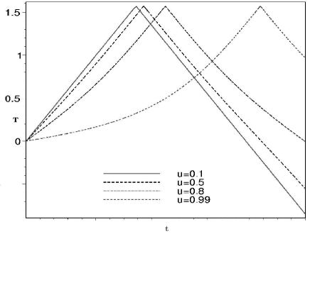
Figure 1: Solution curves for the evolution of the time dependent tachyon ${\tilde{T}}$ with varying values of $u$. The maximum value of the tachyon field is $\pi/2$, which corresponds to the probe brane being stuck to the ring, thus the continuation of the curves beyond the time this happens is unphysical. For simplicity we have set $\sqrt{kl_{s}^{2}}=1$.

We may expect to find a kink solution if we consider the tachyon to be dependent upon a solitary spatial direction, namely $\tilde{T}=\tilde{T}(x)$. In this case the conservation of energy momentum tensor implies

$$\frac{V(\tilde{T})}{\sqrt{1+(\partial_{x}\tilde{T})^{2}}}=\gamma=\rm{constant.}$$ (4.10)

An initial inspection of this equation reveals that there is no kink solution if $u<1$, and that if this constraint becomes an equality then again, the only solution will be $\tilde{T}(x)=0$. From the conservation equation we expect that $\gamma$ will be zero. This is because a kink solution requires $\tilde{T}(x)=\pm\pi\sqrt{kl_{S}^{2}}/2$ for $x\neq 0$, and consequently the potential must be zero. This implies that $\gamma$ is zero since the derivative of $\tilde{T}$ will not be infinite. At $x=0$ we find that the derivative blows up in the denominator, and so once again we find that $\gamma=0$. It will transpire [7] that $\gamma$ is the width of the kink, and since we expect it to be zero this implies that a BPS $D(p-1)$ brane has zero thickness.

If we now proceed with our integration, we find that the solution is given by

$$\tilde{T}(x)=\sqrt{kl_{s}^{2}}\arcsin\left(\frac{\sqrt{u^{2}-1}}{u}Sn\left[\frac{xu}{\sqrt{kl_{s}^{2}}},\frac{\sqrt{u^{2}-1}}{u}\right]\right),$$ (4.11)

where once again $u=\tau_{p}^{u}/\gamma$ and $Sn$ is the Jacobi elliptic function. Now, we make an important observation. For small $\gamma$ we find $u>>1$, and so the second term in the Jacobi function can be approximated by unity. Using the properties of $Sn$, namely that

$$Sn(z,1)=\tanh(z),$$

our expression for the tachyon reduces to

$$T(x)=\sqrt{kl_{s}^{2}}\arcsin\left(\tanh\left[\frac{xu}{\sqrt{kl_{s}^{2}}}\right]\right).$$ (4.12)

This is clearly a kink solution, which interpolates between $\pm\sqrt{kl_{s}^{2}}\pi/2$ due to the arcsin function, for non-zero $x$, whilst at $x=0$ we find $T(x)=0$. Furthermore by differentiating the full solution we find that at $x=0$ we have

$$(\partial_{x}\tilde{T})|_{x=0}=\sqrt{u^{2}-1}$$ (4.13)

This can be made infinite by sending $u$ to infinity, and so we recover the usual solution for tachyonic kinks [7]. In terms of the bulk picture, this corresponds to a brane attached to the ring at $-R$ for $x<0$, and at $+R$ for $x>0$. At $x=0$ we obtain the usual soliton solution which stretches across the diameter of the ring. This kink solution is interesting since the geometrical tachyon only oscillates between the two zeros of the potential, and not the two minima. The open string tachyon also has this behaviour, but it has a runaway potential which is effectively of zero width, whereas the geometrical tachyon potential is clearly of finite width. This is not the case for topological defect solutions in field theory, which tend to stretch from one minima to another in order to be stable. Furthermore, we can compute the energy density ${\cal E}$ of the kink [2, 7, 35] using

$${\cal E}=\int_{-\infty}^{\infty}dxV(\tilde{T})\sqrt{1+(\partial_{x}\tilde{T})^{2}}.$$ (4.14)

In the large $u$ limit we obtain, after some algebra

$${\cal E} = \tau_{p}^{u}\sqrt{kl_{s}^{2}}\int_{-\infty}^{\infty}dy\ \ {\rm sech}^{2}(y)$$ (4.15)

$$= 2\tau_{p}^{u}\sqrt{kl_{s}^{2}}$$

$$= 2R\tau_{p}.$$

Clearly the energy corresponds to a kink solution which is stretched across the diameter of the ring. If we compare this to the energy bound [7] we find

$$T_{\alpha\beta}^{kink}=-\eta_{\alpha\beta}\int_{-\pi\sqrt{kl_{S}^{2}}/2}^{\pi\sqrt{kl_{s}^{2}}/2}d\tilde{T}\ V(\tilde{T}),$$ (4.16)

which reduces to

$$T_{\alpha\beta}=-2\eta_{\alpha\beta}\tau_{p}^{u}\sqrt{kl_{s}^{2}}.$$ (4.17)

Thus we can see that both integrals yield the exact same result, implying that this is the lowest energy state for the brane.

We now investigate what happens when we couple an electric field to the kink, creating a charged soliton. For simplicity we choose a constant electric field which is perpendicular to $\partial_{x}\tilde{T}$, so e.g. $E_{i}=E\delta_{ik}$ where $x^{k}\neq x$ Expanding the action (4.1) for small $\lambda$, and incorporating the factors of $l_{s}^{2}$ into the field definition allows us to write the components of the energy-momentum tensor as

$$T_{\alpha\beta} = -\eta_{\alpha\beta}V(\tilde{T})\sqrt{1-E^{2}+(\partial_{x}\tilde{T})^{2}}$$

$$T_{xx} = \frac{V(\tilde{T})}{\sqrt{1-E^{2}+(\partial_{x}\tilde{T})^{2}}}.$$ (4.18)

There will also be a constant conserved displacement field, which can be derived by varying the action with respect to $\dot{A}_{k}$.

$$D=\frac{EV(\tilde{T})}{\sqrt{1-E^{2}+(\partial_{x}\tilde{T})^{2}}}.$$ (4.19)

We note that using a perturbative expansion in $\lambda$ allows us to consider $E\to 1$, where $E=1$ is the critical value for the field. Using the conservation of $T_{xx}$ we can write

$$E=\frac{D}{\gamma}=\rm{constant.}$$ (4.20)

The presence of the electric field modifies the kink solution only slightly, find

$$\tilde{T}(x)=\sqrt{kl_{s}^{2}}{\rm arcsin}\left(\frac{\sqrt{u^{2}+E^{2}-1}}{u}Sn\left[\frac{xu}{\sqrt{kl_{s}^{2}}},\frac{\sqrt{u^{2}+E^{2}-1}}{u}\right]\right).$$ (4.21)

There is an interesting case where the electric field takes its critical value, as we no longer have to consider the large $u$ limit in our solution since it reproduces (4.12). This generally implies that the kink solution can be non-singular. If we allow $u=1$ in the full solution, then the tachyon is entirely dependent upon $E$. In fact it reduces to

$$T(x)=\sqrt{kl_{s}^{2}}\arcsin\left(ESn\left[\frac{x}{\sqrt{kl_{s}^{2}}},E\right]\right).$$ (4.22)

Using the expansion properties of the Jacobi function we find that for $E$ close to unity, we have a solitary kink solution of finite width, whilst for small $E$ we find an tiny array of small kink-antikink solutions which have period $x=2n\pi\sqrt{kl_{s}^{2}}$. We want to know which of these solutions are stable, so we must integrate the energy momentum tensor over the $x$ direction on the world sheet. The final result is

$$T_{\alpha\beta}=-2\eta_{\alpha\beta}\tau_{p}^{u}\sqrt{kl_{s}^{2}}{\rm EllipticE}\left(\frac{\sqrt{u^{2}+E^{2}-1}}{u}\right),$$ (4.23)

where we have used the periodic properties of the Jacobi functions. This clearly shows us that the minimum energy configuration occurs when

$$\frac{(u^{2}+E^{2}-1)}{u^{2}}=1$$ (4.24)

which implies that $u\to\infty$ or $E=1$. The first case corresponds to the uncharged kink solution of infinitesimal width, implying that the electric flux is diluted to the point where it is effectively zero. The second solution requires that the electric field takes its critical value, and the resulting kink solution can be deformed to one of finite width. Furthermore all the possible kink configurations will have the exact same energy. Thus the introduction of electric flux introduces a fixed point into the theory, since a small electric field will find it energetically more favourable to increase to its maximum size. This tells us that the stable kink solutions will either be uncharged, or fully charged under the $U(1)$ gauge field.

Interestingly, in the time dependent kink solution with a critical field strength, we find that $\tilde{T}(t)=\sqrt{kl_{s}^{2}}\pi/2$ for all time, corresponding to the probe brane being permanently attached to the ring. This is to be expected since flux on the brane effectively increases the ’mass’, forcing the probe further into the throat generated by the fivebranes [26].

5 Non-BPS branes.

The existence of the unstable $Dp$-brane at the point $\rho=0,\sigma=0$ is reminiscent of a Non-BPS brane. Thus it is useful to construct the solution for a Non-BPS brane in this ring background. Recall that a $Dp$ Non-BPS brane is related to a BPS $D(p-1)$ brane, since the latter is a soliton on the world-volume of the former. The Non-BPS brane action is similar to the usual DBI governing the behaviour of the BPS $Dp$-brane, except that it has a tachyon on its world-volume, and an additional tachyon potential. The action is of the form

$$S=-\int d^{p+1}\zeta V(T)\sqrt{-det(G_{\mu\nu}+\partial_{\mu}T\partial_{\nu}T)}.$$ (5.1)

The form of the action suggests that the tachyon is effectively playing the role of an extra direction in field space. Into this action we want to substitute our $NS$5-brane background, which can easily be shown to yield

$$S=-\int d^{p+1}\zeta\frac{V(T)}{\sqrt{H}}\sqrt{-det(\eta_{\mu\nu}+H\partial_{\mu}X^{m}\partial_{\nu}X_{m}+\partial_{\mu}T\partial_{\nu}T)}.$$ (5.2)

Where we use static gauge, and the $X^{m}$ are the transverse scalars. We now use the tachyon map to redefine the radion field, recalling that $\tilde{T}$ is the geometrical tachyon the action becomes:

$$S=-\int d^{p+1}\zeta V(T,\tilde{T})\sqrt{-det(\eta_{\mu\nu}+\partial_{\mu}T\partial_{\nu}T+\partial_{\mu}\tilde{T}\partial_{\nu}\tilde{T})}.$$ (5.3)

Note that we are able to couple the two tachyon potentials together, with $V(T,\tilde{T})=V(T){\tilde{V}}(\tilde{T})$, ${\tilde{V}}(\tilde{T})$ being the potential of the geometric tachyon. This is already suggestive of something interesting. The geometrical tachyon potential is that already derived in (3.8). We will try and remain general about the form of the tachyon potential $V(T)$ by insisting that it meets the criteria described in the previous section. Note that this behaviour is easily satisfied by the $1/\cosh(T/\sqrt{2})$ potential [12, 13]. In addition we note that the form of the action allows the two tachyons to decouple from each others equation of motion. Thus we may look at the dynamics by explicitly solving these equations, or by conservation of the energy momentum tensor. The form of the action in (5.3) suggests that we could define a complex tachyon field given by $U=T+i\tilde{T}$, however for the purpose of this note we will not do so. This is usually done when we have a $Dp$ and a $\bar{Dp}$-brane and are looking for vortex solutions. It would of course be interesting to see what the effects of this redefinition would mean in terms of the general behaviour of the probe motion.

We can now proceed with our analysis of solutions to the equations of motion for the non-BPS action.

5.1 One spatial direction.

To begin with we will consider the simple case where $T=T(x)$ and $\tilde{T}=\tilde{T}(x)$, where $x$ is an arbitrary direction on the world-volume. Here and in the remainder of the section we shall set $l_{s}^{2}=1$. Denoting the derivative with respect to $x$ by a prime, we can write the action as follows.

$$S=-\int d^{p+1}\zeta V(T,\tilde{T})\sqrt{1+T^{{}^{\prime}2}+{\tilde{T}}^{{}^{\prime}2}}$$ (5.4)

which allows us to calculate the associated energy momentum tensor, with components

$$T_{\alpha\beta} = -\eta_{\alpha\beta}V(T,\tilde{T})\sqrt{1+T^{{}^{\prime}2}+{\tilde{T}}^{{}^{\prime}2}}$$

$$T_{xx} = \frac{-V(T,\tilde{T})}{\sqrt{1+T^{{}^{\prime}2}+{\tilde{T}}^{{}^{\prime}2}}}$$ (5.5)

Where $\alpha,\beta$ run over the $0,2\ldots p-1$ directions perpendicular to $x$. We will assume that the open string tachyon has the usual kink solution, namely that as $x\to\pm\infty$, $T(x)\to\pm\infty$ and $V(T)\to 0$. Using the conservation of the energy momentum tensor, $\partial_{x}T_{xx}=0$   $\forall x$, we see that this is automatically satisfied by the kink solution since the open string tachyon component of the potential rolls to zero as the tachyon condenses. Furthermore, this is true irrespective of the behaviour of the geometrical tachyon. In fact it turns out that the $xx$ component of the tensor must vanish for all $x$, not just the derivative [7], [14]. In any case, this physically corresponds to the appearance of a codimension 1 brane located at the origin of the ring. This is just the BPS $D(p-1)$ probe brane used to probe the background [21]. Alternatively we may find that the geometrical tachyon condenses first. In which case the brane will be stretched across the diameter of the ring, leaving an unstable soliton at the origin. It would be interesting to see what happens when both fields condense at the same time.

5.2 Two (or more) spatial directions.

We can now extend the analysis to consider dependence upon two (or more) spatial directions, namely $T=T(x)$, $\tilde{T}=\tilde{T}(y_{j})$, where $j=2\ldots p+1$. The associated components of the energy momentum tensor are

$$T_{\alpha\beta} = -\eta_{\alpha\beta}V(T,\tilde{T})\sqrt{(1+(\partial_{x}T)^{2})(1+(\partial_{y_{j}}\tilde{T})^{2})}$$

$$T_{xx} = -V(T,\tilde{T})\frac{\sqrt{1+(\partial_{y_{j}}\tilde{T})^{2}}}{\sqrt{1+(\partial_{x}T)^{2}}}$$

$$T_{y_{j}y_{j}} = -V(T,\tilde{T})\frac{\sqrt{1+(\partial_{x}T)^{2}}}{\sqrt{1+(\partial_{y_{j}}\tilde{T})^{2}}}.$$ (5.6)

Now we find there are two conservation conditions, $\partial_{x}T_{xx}=0$ and $\partial_{y_{j}}T_{y_{j}y_{j}}=0$. These simply state that $T_{xx}$ is independent of $x$ and $T_{y_{j}y_{j}}$ is independent of the $y_{j}$’s. We look for the usual tachyon kink solution in the $x$ direction, which satisfies both conditions in the limit that $x\to\pm\infty$. At the point $x=0$ we expect that the derivative of the tachyon field becomes infinite, which means that $T_{xx}$ vanishes. But there is still the conservation of $T_{y_{j}y_{j}}$ to consider. In order for this to hold for all $y_{j}$ we must ensure that ${\tilde{V}}(\tilde{T})\to 0$, which means that the geometrical tachyon must also condense. But this tachyon also has a kink solution associated with it, and so the conservation conditions are automatically satisfied.

We know that the condensation of the open string tachyon yields a BPS $D(p-1)$ brane, but we may well enquire about what the condensation of the geometrical tachyon correspond to? Naively we may assume that it gives rise to a Non-BPS $D(p-2)$-brane, but this brane would be unstable and have no tachyonic modes left which could condense and stabilise it.

More generally, using the factorization properties of the Non-BPS brane action, we may write the brane descent relations for both kink solutions and find the energy,

$${\cal E}=\int_{-\infty}^{\infty}V(T)dT\int_{-\pi\sqrt{k}/2}^{\pi\sqrt{k}/2}{\tilde{V}}(\tilde{T})d\tilde{T}.$$ (5.7)

In order to do this we first specify the form of the tachyon potential, which we will take to be

$$V(T)=\frac{\tau_{p}^{non}}{\cosh(\frac{T}{\sqrt{2}})}.$$ (5.8)

with $\tau_{p}^{non}$ the non-BPS brane tension. The first integration yields

$${\cal E}=\pi\sqrt{2}\tau_{p}^{non}\int_{-\pi\sqrt{k}/2}^{\pi\sqrt{k}/2}{\tilde{V}}(\tilde{T})d\tilde{T}$$ (5.9)

However, we have already seen that the configuration of the BPS D(p-1) brane is itself unstable due to the geometrical tachyonic mode also forming a kink. If we integrate over this potential we find

$${\cal E}=2\pi R\tau_{p}^{non}\sqrt{2}$$ (5.10)

This can be written as

$${\cal E}=(2R\tau_{p})\times 2\pi$$ (5.11)

where we have used the relation $\tau_{p}^{non}=\sqrt{2}\tau_{p}$, $\tau_{p}$ being the BPS Dp brane tension [34]. One possible interpretation of the form of the energy (5.11)is as follows. The first factor in (5.11) is the energy of Dp brane stretched along the diameter of the ring, which we calculated earlier (4.15). The additional factor of $2\pi$ can be thought of as coming from ’smearing’ the stretched brane around the inside of the ring.

5.3 Space and time dependence.

We assume that the geometrical tachyon is time dependent, whilst the open string tachyon is spatially dependent. This allows us to write the the components of the energy momentum tensor as

$$T_{00} = V(T,\tilde{T})\frac{\sqrt{1+(\partial_{x}T)^{2}}}{\sqrt{1-(\partial_{0}\tilde{T})^{2}}}$$

$$T_{ij} = -\delta_{ij}V(T,\tilde{T})\sqrt{(1+(\partial_{x}T)^{2})(1-(\partial_{0}\tilde{T})^{2})}$$

$$T_{xx} = -V(T,\tilde{T})\frac{\sqrt{1-(\partial_{0}\tilde{T})^{2}}}{\sqrt{1+(\partial_{x}T)^{2}}}.$$ (5.12)

We again appeal to the conservation equations to determine the behaviour of the kink solution. If we assume there is a kink in the $x$ direction, then we find that there are only two possibilities for the geometrical tachyon. We either have a kink in the time direction, or the field must condense. Since we have already established that there is no stable kink solution, we again find that the tachyon condenses, and this implies that the $Dp$-brane moves toward the ring. Looking explicitly at the conservation equation for the $T_{xx}$ component we find the expected decoupling behaviour

$$\partial_{x}\left(\frac{V(T)}{\sqrt{1+(\partial_{x}T)^{2}}}\right)=0.$$ (5.13)

This allows us to integrate the equation to determine the $x$ dependence of the open string tachyon, provided we specify the explicit form of the potential. If we choose the usual form (5.8) then upon integration we obtain the solution

$$\sinh\left(\frac{T}{\sqrt{2}}\right)=\frac{\sqrt{1-p^{2}}}{p}\sin\left(\frac{x}{\sqrt{2}}\right)$$ (5.14)

where $p$ is an arbitrary constant of integration. If we now substitute for $\partial_{x}T$ in the $T_{00}$ component of the stress tensor we find

$$T_{00}=\frac{{\tilde{V}}(\tilde{T})}{\sqrt{1-(\partial_{0}\tilde{T})^{2})}}\frac{p}{p^{2}+(1-p)^{2}{\rm sin}^{2}\left(\frac{x}{\sqrt{2}}\right)}.$$ (5.15)

This is the same result that Kluson derived for branes moving on a transverse $\mathbf{R}^{3}\times\mathbf{S}^{1}$, and can be interpreted as an array of $D(p-1)$-branes and $D(p-1)$-antibranes. Since there is a map between the rolling of the time dependent geometrical tachyon and the motion of a probe $Dp$-brane we can see that these branes simply move toward the ring.

6 Compactification in a transverse direction.

In [2] Kutasov established the relationship between BPS and Non-BPS branes by compactifying one of the transverse directions in the coincident $NS$5-brane background. Since we have already seen that geometric tachyons can exist when the brane is probing a compact space, we may well enquire if there will be tachyonic modes if we compactify one of the transverse directions in the ring background.

Due to the symmetry of the transverse space, it is easiest to consider a compactification in the $\sigma$ plane. We remind the reader of the harmonic function in this instance (3.16)

$$H(\sigma)=\frac{kl_{s}^{2}}{R^{2}+\sigma^{2}}.$$ (6.1)

We will choose to compactify the $x_{8}$ direction into a circle of radius $L$. The resultant expression for the harmonic function becomes

$$H=\sum_{m=-\infty}^{\infty}\frac{kl_{s}^{2}}{(R^{2}+x_{9}^{2})+(x_{8}-2\pi Lm)^{2}}.$$ (6.2)

This sum is easy to do, since it is very similar in form to the one in [2], and we obtain the final form of the function

$$H=\frac{kl_{s}^{2}}{2L|z|}\frac{\sinh(|z|/L)}{(\cosh(|z|/L)-\cos(y/L)),}$$ (6.3)

where we have defined $z=\sqrt{R^{2}+x_{9}^{2}}$ and $y=x_{8}$. In this form the harmonic function is exactly the same as that for a coincident fivebrane background, except that if we set the $x_{9}$ fields to their minimum value we find $z=R$.

Performing the tachyon map integration we obtain the following solution for the tachyon

$$\tilde{T}(y)=\sqrt{\frac{2Lkl_{s}^{2}\sinh(|z|/L)}{|z|(1+a)}}\rm{EllipticF}(\delta,r)$$ (6.4)

where EllipticF is the incomplete elliptic integral of the second kind and we have made the following definitions:

$$a = \cosh(|z|/L)$$

$$\delta = \arcsin\left(\sqrt{\frac{(1+a)(1-\cos(y/L))}{2(a-\cos(y/L))}}\right)$$ (6.5)

$$r = \sqrt{\frac{2}{1+a}}.$$

By setting the $x_{9}$ fields to zero we see that the behaviour of the tachyon is dependent upon the ratios $R/L$ and $y/L$. We can see that as $y\to 0$, the numerator of $\delta\to 0$ and using the properties of elliptic integrals we find that $\tilde{T}\to 0$. This is to be expected since [2] essentially argues the same thing, namely that the tachyon starts at some initial value $\tilde{T}=\tilde{T}_{max}$ at the point $y=\pi L$, and then rolls toward zero as $y\to 0$. However we see that there is also the ratio $R/L$ in the tachyon solution, which we would expect to explicitly determine the value of $\tilde{T}$ since this term dominates the cosine term associated with the motion around the compact dimension. We can calculate the maximum value for the tachyon

$$\tilde{T}_{max}=\sqrt{\frac{2Lkl_{s}^{2}\sinh(R/L)}{R(1+\cosh(R/L))}}{\rm EllipticK}\left(\sqrt{\frac{2}{1+{\rm cosh}(R/L)}}\right),$$ (6.6)

where we have introduced the elliptic integral of the first kind. We can make some approximations to determine the behaviour of the field. Firstly we take the limit $R/L<<1$

$$\tilde{T}_{max}\approx\sqrt{\frac{2Lkl_{s}^{2}\sinh(R/L)}{R(1+\cosh(R/L))}}\ln\left(4\sqrt{\frac{1+\cosh(R/L)}{\cosh(R/L)-1}}\right)$$ (6.7)

which can be seen to tend to infinity. In the converse limit we can approximate the tachyon field by

$$\tilde{T}\approx\sqrt{\frac{2Lkl_{s}^{2}}{R}}\arcsin\left(\sqrt{\frac{a(1-{\rm cos}(y/L))}{2(a-{\rm cos}(y/L))}}\right).$$ (6.8)

which yields a maximum value of

$$\tilde{T}_{max}\approx\sqrt{\frac{2Lkl_{s}^{2}}{R}}\frac{\pi}{2},$$ (6.9)

and will roll to zero as $y\to 0$. Clearly the maximum value of the tachyon field will be determined by the exact ratio of $R/L$ and also the number of source branes.

We can also determine the tachyon potential in this instance by inverting the solution (6.4). After some manipulation using elliptic functions we obtain

$$\tilde{V}(\tilde{T})=\sqrt{\frac{2LR}{kl_{s}^{2}\sinh(R/L)}}\sqrt{\frac{(1-a)(1+a)}{1-a-2Sn^{2}[\Delta(\tilde{T}),r]}}.$$ (6.10)

where $a$ and $r$ are the same as before, whilst $\Delta(\tilde{T})$ is defined to be

$$\Delta(\tilde{T})={\tilde{T}}\sqrt{\frac{R(1+a)}{kl_{s}^{2}L\sinh(R/L)}}.$$

This is a complicated potential, and does not yield simple analytic solutions. Furthermore we see that it is not defined for $R/L<<1$ or even $R\approx L$ due to the presence of the Jacobi function in the denominator. Thus, it is only valid for the $R/L>>1$ case and we must also assume that the tachyon never becomes too large! The potential can only be zero if $L=0$ which means that the compact dimension is of zero size, and a probe brane moving along it will be essentially stuck at the origin. For all other values of $R$ and $L$ the minimum of the potential is at some fixed non-zero value. The unstable maximum of the potential should occur when $\tilde{T}=\tilde{T}_{max}$. For the case when $R/L>>1$ we find that

$$V_{max}(\tilde{T})\approx\sqrt{\frac{2LR\cosh(R/L)}{kl_{s}^{2}\cosh(R/L)+2\tilde{T}^{2}R}}.$$ (6.11)

As the tachyon field decreases, the potential decreases, passing through its minimum at $\tilde{T}=0$ which in the brane picture corresponds to the probe passing through the origin. Thus we anticipate that the tachyon field in this instance will be massive, as it was for the case in an earlier section. This again suggests that we will obtain massive fields when we compactify, unless the compact space is bounded by fivebranes.

Compactifying one of the directions in the plane of the ring is also possible, however we will not consider it here. The main difficulty lies in the fact that there is a crossover between harmonic functions in different regions of the covering space, but there is also the additional problem of the complicated form of the functions. It appears likely that there will be a geometrical tachyon in this instance when the probe is confined to the region $y=R\ldots 2\pi L-R$, since it is bounded by $NS$5 branes. But there is also the possibility of new geometrical tachyons in the region $2\pi L-R\ldots R$ which should map onto the tachyon field discussed earlier. Once again we would expect the ratio $R/L$ to fully specify the tachyon dynamics.

7 Discussion.

We have investigated the dynamics of a BPS $Dp$-brane in the background of a ring of coincident $NS$5-branes from the perspective of a rolling tachyon on the brane world volume. We have seen that the radial mode associated with brane motion inside the ring gives rise to a ’geometrical tachyon’ on the brane, complete with a tachyon potential which describes the changing tension.

Although we do not find a kink solution in the time-like direction, we can find exact solutions for the rolling behaviour which are equivalent to the equations of motion for the probe $Dp$-brane. Thus mapping the action to a different form can simplify the problem.

We do find a spatial kink solution which appears to be stable on its own. It still remains to be seen whether there are any stable vortex solutions. Additionally if one of the dimensions of the probe brane is wrapped on a circle then other kinds of non-singular kink solutions are possible. It may be interesting to investigate this and compare the results with those for the open string tachyon. If the kink is charged, we would anticipate there to be a wide variety of solutions such as kink-antikink arrays. Furthermore we have probed the background geometry with a Non-BPS brane, which has an open string tachyon on its world-volume. As expected, the kink solution describes the existence of a BPS $D(p-1)$-brane but the condensation of the geometrical tachyon implies that this brane is somehow smeared around the interior of the ring.

We have seen that there are no geometrical tachyons if we compactify one of the transverse directions to the ring in the limit of $R/L>>1$. This is because the compact space is not bounded by the fivebranes. In the converse limit $R/L<<1$ we find the theory breaks down because the ’tachyonic field’ becomes infinite. If we were to compactify along the plane of the ring, then we would expect to see two tachyonic modes, one of which should map to the one discussed in this paper.

This analysis raises several questions about the nature of the open string tachyon in string theory, and we can make several useful observations. Firstly we have found that a compact space is not enough to create geometrical tachyons. The space must be bound at either end by fivebranes, implying that the radion field is bound between a range of values. In [2, 34] this corresponds to branes located at $y=0$ and $y=2\pi R$ on a compact circle whilst in the ring case it corresponds to branes at $-R$ and $R$ at opposite points of the circle. Secondly we must ensure that the compact space is symmetric about the unstable point of the potential, to ensure that the tachyon can condense. This is equivalent to saying that the potential must be an even function. Thirdly it appears that geometrical tachyons can give rise to stable kink solutions on their own, but not when we include another tachyonic field. The form of the potential is dependent solely upon the background spacetime geometry. It would be interesting to consider other background geometries and find different tachyonic potentials. This could be especially useful for cosmology, since hybrid inflation requires the condensation of two scalar fields.

It can also be shown that if we S-dualize the background solution to obtain a ring of $D5$-branes, we obtain similar geometrical tachyonic modes for a probe $Dp$-brane with $p=3$ and $p=5$. The $p=3$ case is the exact S-dual of the configuration in this note, however the $p=5$ case has a tachyon potential given by $V(\tilde{T})=\tau_{p}^{u}(\cos^{2}(\tilde{T}/\sqrt{k}))$ where $k$ is a constant given in terms of the string length, string coupling and the number of branes. This is not a truncated tachyon potential, and so we may find stable kink solutions even when coupled to open string tachyons. It would be useful to analyse this and the corresponding S-dual solution for $\mathbf{R}^{3}\times\mathbf{S}^{1}$ in the coincident background to see if there are kink solutions, and what their implications are for the rolling tachyon.

Finally, the emergence of a cosine potential for the geometric tachyon inside the ring might have interesting applications to inflationary cosmology. Similar potentials have been argued to lead to so called natural-inflation [42]. In our case the scales $\sqrt{kl_{s}^{2}}$ and $R$ of geometric tachyon potential (4.2) might play similar roles to $\Lambda$ and $f$ in [42].However given the non-linearities of the DBI action a direct comparison of the tachyon potential and the cosine inflaton potentials is delicate. Rather, an analysis of the tachyon cosmology following e.g.[43] and [44] should be carried out.

Acknowledgements.

Many thanks go to Costis Papageorgakis for participating in several useful conversations and to Konstadinos Sfetsos for useful comments.

References

- [1] David Kutasov, ’D-brane Dynamics Near NS5 branes’, hep-th/0405058.
- [2] David Kutasov, ’A Geometric Interpretation of the Open String Tachyon’, hep-th/0408073.
- [3] D. Kutasov and V. Niarchos, ’Tachyon effective actions in open string theory’, hep-th/0304045, Nucl. Phys. D 69, 106009 (2004).
- [4] David A. Sahakyan, ’Comments on D-brane Dynamics Near NS5-Branes’, hep-th/0408070.
- [5] A. Sen, ’Rolling Tachyon’, hep-th/0203211, JHEP 0204 (2002) 048.
- [6] A. Sen ’Field Theory of Tachyon Matter’, hep-th/0204143, Mod. Phys. Lett A 17 (2002), 1797-1804
- [7] A. Sen, ’Dirac-Born-Infeld Action on the Tachyon Kink and Vortex’, hep-th/0303057, Phys. Rev D 68 (2003) 066008.
- [8] A. Sen, ’Supersymmetric world-volume action for non-BPS D-branes’, hep-th/9909062, JHEP 9910 (1999) 008.
- [9] J. Kluson, ’Proposal for non-BPS D-brane action’, hep-th/0004106, Phys. Rev. D 62 (2000) 126003.
- [10] E. A. Bergshoeff, M. de Roo, T. C. de Wit, E. Eyras and S. Panda, ’T-duality and actions for non-BPS D-branes’, hep-th/0003221, Nucl. Phys. B 584 (2000) 284.
- [11] M. R. Garousi, ’Tachyon couplings on Non-BPS D-branes and Dirac-Born-Infeld action’, hep-th/0003122, Nucl. Phys B 584 (2000), 284-299.
- [12] D. Kutasov and V. Niarchos, ’Tachyon effective actions in open string theory’, hep-th/0304045, Nucl. Phys. B 666 (2003) 56.
- [13] N. Lambert, H. Liu and J. Maldacena, Closed strings from decaying D-branes’, hep-th/0303139.
- [14] C. Kim, Y. Kim, O. K. Kwon, C. O. Lee, ’Tachyon kinks on unstable DP-branes’, hep-th/0305092, JHEP 0311 (2003) 115.
- [15] C. Kim, Y. Kim and C. O. Lee, ’Tachyon kinks’, hep-th/0304180, JHEP 0305 (2003) 020.
- [16] P. Brax, J. Mourad and D. A. Steer, ’Tachyon kinks on non BPS D-branes’, hep-th/0304197, Phys. Lett. B 575 (2003) 115.
- [17] P. Brax, J. Mourad and D. A. Steer, ’On Tachyon kinks from the DBI action’, hep-th/0310079.
-
[18]
Konstadinos Sfetsos, ’Branes for Higgs Phases and Exact Conformal Field Theories’,
hep-th/9811167, JHEP 9901 (1999) 015.
Konstadinos Sfetsos, ’On (multi) center branes and exact string vacua’, hep-th/9812165.
Konstadinos Sfetsos, ’Rotating NS5-brane solution and its exact string theoretic description’, hep-th/9903201, Fortsch. Phys, 48, 199 (2000). - [19] M. Gutperle and A. Strominger, ’Spacelike Branes’, hep-th/0202210, JHEP 0204 (2002) 018.
- [20] J. Wang, ’Spacelike and Time Dependent Branes from DBI’, hep-th/0207089, JHEP 0210 (002) 005.
- [21] S. Thomas and J. Ward, ’D-Brane Dynamics and NS5 Rings’, hep-th/0411130.
- [22] Y. Nakayama, Y. Sugawara and H. Takayanagi, ’Boundary states for the rolling D-branes in NS5-background’ , hep-th/0406173, JHEP 0407 (2004) 020.
- [23] Y. Nakayama, K. Panigrahi, S. J. Rey and H. Takayanagi, ’Rolling Down the Throat in NS5-Brane Background: The case of Electrified D-Brane’, hep-th/0412038.
- [24] B. Chen, M. Li and B. Sun, ’Dbrane Near NS5-branes: with Electromagnetic Field’, hep-th/0412022, JHEP 0412 (2004) 057.
- [25] B. Chen and B. Sun ’Note on DBI dynamics of Dbrane Near NS5-branes’, hep-th/0501176.
- [26] S. Thomas and J. Ward ’D-brane dynamics near compactified NS5-branes’, hep-th/0501192.
- [27] D. Bak, S. J. Rey and H. U Yee, ’Exactly soluble Dynamics of (p,q) String Near Macroscopic Fundamental Strings’, hep-th/0411099, JHEP 0412 (2004) 008.
- [28] Ahmad Ghodsi and Amir E. Mosaffa, ’D-brane Dynamics in RR deformation of NS5-branes Background and Tachyon Cosmology’, hep-th/0408015.
- [29] Hossein Yavartanoo, ’Cosmological Solution from D-brane motion in NS5-branes background’, hep-th/0407079.
- [30] Kamal L. Panigrahi, ’D-Brane Dynamics in Dp-Brane Background’, hep-th/0407134, Phys. Lett. B 601 (2004) 64-72.
- [31] O. Saremi, L. Kofman and A. W. Peet, ’Folding Branes’, hep-th/0409092.
- [32] C. G. Callan, J. A. Harvey and A. Strominger, ’Supersymmetric string solitons’, hep-th/9112030.
- [33] J. Kluson, ’Non-BPS D-Brane Near NS5-Branes’, hep-th/0409298, JHEP 0411 (2004) 013.
- [34] J. Kluson, ’Non-BPS Dp-Brane in the background of NS5-Branes on Transverse ’, hep-th/0411014.
- [35] J. Kluson, ’Non-BPS Dp-Brane In Dk-Brane Background’, hep-th/0501010.
- [36] J. Kluson, ’Note About Non-BPS and BPS Dp-branes in Near Horizon Region of N Dk-branes’, hep-th/0502079.
- [37] J. A. Minahan and B. Zwiebach, ’Effective tachyon Dynamics in Superstring Theory’, hep-th/0009246, JHEP 0103 (2001) 038.
- [38] A. A. Gerasimov and S. L. Shatashvili, ’On Exact Tachyon Potential in Open String Field Theory’, hep-th/0009103, JHEP 0010 (2000) 034.
- [39] C. P. Burgess, P. Martineau, F. Quevedo and R. Rabadan, ’Branonium’, hep-th/0303170, JHEP 0306 (2003) 037.
- [40] C. P. Burgess, N. E. Grandhi, F. Quevedo and R. Rabadan, ’D-brane Chemistry’, hep-th/0310010, JHEP 0401 (2004) 06.
- [41] W. Huang, ’Tubular Solutions in NS5-brane, Dp-brane and Macroscopic Strings Background’. hep-th/0502023.
- [42] K.Freese, J.A. Frieman and A.V.Olinto, ‘Natural Inflation’, Phys. Rev. Lett. 65, 3233 (1990). K.Freese and W.H.Kinney, ‘On Natural Inflation’, hep-th/0404012, Phys.Rev. D70 (2004) 083512.
- [43] G.W.Gibbons, ‘Cosmological Evolution of the Rolling Tachyon’, hep-th/0204008, Phys.Lett. B537 (2002) 1-4. ‘Thoughts on Tachyon Cosmology’, hep-th/0301117, Class.Quant.Grav. 20 (2003) S321-S346.
- [44] X-Z. Li, D-J Liu and J-G Hao, ‘On the tachyon inflation’, hep-th/0207146, J. Shanghai Normal Univ. (Natural Sciences), Vol. 33(4), (2004), 29.