Twistor cosmology and quantum space-time

Abstract

The purpose of this paper is to present a model of a ‘quantum space-time’ in which the global symmetries of space-time are unified in a coherent manner with the internal symmetries associated with the state space of quantum-mechanics. If we take into account the fact that these distinct families of symmetries should in some sense merge and become essentially indistinguishable in the unified regime, our framework may provide an approximate description of or elementary model for the structure of the universe at early times. The quantum elements employed in our characterisation of the geometry of space-time imply that the pseudo-Riemannian structure commonly regarded as an essential feature in relativistic theories must be dispensed with. Nevertheless, the causal structure and the physical kinematics of quantum space-time are shown to persist in a manner that remains highly analogous to the corresponding features of the classical theory. In the case of the simplest conformally flat cosmological models arising in this framework, the twistorial description of quantum space-time is shown to be effective in characterising the various physical and geometrical properties of the theory. As an example, a sixteen-dimensional analogue of the Friedmann-Robertson-Walker cosmologies is constructed, and its chronological development is analysed in some detail. More generally, whenever the dimension of a quantum space-time is an even perfect square, there exists a canonical way of breaking the global quantum space-time symmetry so that a generic point of quantum space-time can be consistently interpreted as a quantum operator taking values in Minkowski space. In this scenario, the breakdown of the fundamental symmetry of the theory is due to a loss of quantum entanglement between space-time and internal quantum degrees of freedom. It is thus possible to show in a certain specific sense that the classical space-time description is an emergent feature arising as a consequence of a quantum averaging over the internal degrees of freedom. The familiar probabilistic features of the quantum state, represented by properties of the density matrix, can then be seen as a by-product of the causal structure of quantum space-time.

1 Introduction

This article is concerned with a programme that has as its goal the development of a theory of quantum space-time. In this programme, an outline of which will be given in more detail shortly, an important role is played by certain higher-dimensional analogues of spinors and twistors. It will be useful to begin, therefore, by remarking that there are two distinct notions of how one extends the concept of spinor into higher dimensions. This fundamental dichotomy arises in association with the fact that in four-dimensional space-time there is a local isomorphism between the Lorentz group $SO(1,3)$ and the spin transformation group $SL(2,{\mathbb{C}})$. In higher dimensions, however, this relation breaks down and as a consequence we are left with two concepts of spinors—one for the group $SO(N,{\mathbb{C}})$, and one for the group $SL(r,{\mathbb{C}})$.

The spinors associated with $SO(N,{\mathbb{C}})$, where we allow also for various possible signatures in the quadratic form defining these orthogonal or pseudo-orthogonal transformations when we specialise to the real subgroup $SO(p,q)$ with $p+q=N$, are the so-called Cartan spinors Budinich ; Cartan ; Chevalley ; Penrose9 . The study of Cartan spinors has a long and interesting history, and there is a beautiful geometry associated with these spinors. There are also various specific cases of great interest—for example, the Cartan spinors associated with the group $SO(2,4)$ are Penrose’s twistors; and the Cartan spinors associated with $SO(8)$ are intimately linked with the Cayley numbers (octonions) and the exceptional Lie groups. There are also a number of interesting connections between Cartan spinors and massless fields in higher dimensions Hughston4 ; Hughston6 ; Hughston5 .

The spinors associated with $SL(r,{\mathbb{C}})$, which are usually now called ‘hyperspinors’, have the advantage of being more directly linked with quantum mechanics. In fact, we shall show later that a naturally relativistic model for hyperspin arises when one considers ‘multiplets’ of two-component spinors, i.e. expressions of the form $\xi^{{\bf A}i}$ and $\eta^{{\bf A}^{\prime}}_{i}$, where ${\bf A},{\bf A}^{\prime}$ are standard spinor indices, and $i=1,2,\ldots,n$ is an ‘internal’ index. In the general case ($n=\infty$) we then think of $\xi^{{\bf A}i}$ as an element of the tensor product space ${\mathbb{S}}^{{\bf A}i}={\mathbb{S}}^{\bf A}\otimes{\mathbb{H}}^{i}$, where ${\mathbb{S}}^{\bf A}$ is the complex vector space of two-component spinors, and ${\mathbb{H}}^{i}$ is an infinite-dimensional complex Hilbert space.

There is also a link, arising through a further extension of this idea, between hyperspinor theory and the theory of multi-twistor (hypertwistor) systems. Indeed, we find that the theory of hyperspin constitutes a natural starting place for building up a theory of quantum geometry or, as we shall call it here, quantum space-time. In summary, we shall be taking the left-hand path in the following diagram:

The hyperspinor route has the virtue that the resulting space-time has a rich causal structure associated with it, and as a consequence is unusually well-positioned to form the geometrical basis of a physical theory.

2 Relativistic causality

To start, let us review briefly the role of two-component spinors in the description of four-dimensional Minkowskian space-time geometry. In what follows we use bold upright Roman letters to denote two-component spinor indices, and we adopt the standard conventions for the algebra of two-component spinors Penrose2 ; Penrose8 ; Penrose9 ; Pirani . Then we have the following correspondence between two-by-two Hermitian matrices and space-time points, relative to some origin:

$$x^{{\bf AA}^{\prime}}\quad({\bf A},{\bf A}^{\prime}=1,2)\qquad\longleftrightarrow\qquad x^{\rm a}\quad({\rm a}=0,1,2,3).$$ (1)

More explicitly, in a standard basis this correspondence is given by

$$\frac{1}{\sqrt{2}}\left(\begin{array}[]{ll}t+z&x+{\rm i}y\\ x-{\rm i}y&t-z\end{array}\right)\quad\longleftrightarrow\quad(t,x,y,z).$$ (4)

We then have the fundamental relation

$$2\det(x^{{\bf AA}^{\prime}})=t^{2}-x^{2}-y^{2}-z^{2},$$ (5)

from which it follows that two-component spinors are connected both with quantum mechanics and with the causal structure of space-time. It is a peculiar aspect of relativistic physics that there is this link between (a) the spin degrees of freedom of spin one-half particles, and (b) the causal geometry of four-dimensional space-time.

Let us pursue this idea now in a little more detail, and then extend it to higher dimensions. For the interval $r^{{\bf AA}^{\prime}}$ between a pair of points $x^{{\bf AA}^{\prime}}$ and $y^{{\bf AA}^{\prime}}$ in Minkowski space-time we write

$$r^{{\bf AA}^{\prime}}=x^{{\bf AA}^{\prime}}-y^{{\bf AA}^{\prime}},$$ (6)

from which it follows that

$$2\det(r^{{\bf AA}^{\prime}})=\epsilon_{\bf AB}\epsilon_{{\bf A}^{\prime}{\bf B}^{\prime}}r^{{\bf AA}^{\prime}}r^{{\bf BB}^{\prime}},$$ (7)

where $\epsilon_{\bf AB}$ is the antisymmetric spinor. Hence if we adopt the standard ‘index clumping’ convention and write ${\rm a}={\bf AA}^{\prime}$, ${\rm b}={\bf BB}^{\prime}$, and so on, according to which a pair of spinor indices, one primed and the other unprimed, corresponds to a lower case space-time vector index, then we can write

$$\epsilon_{\bf AB}\epsilon_{{\bf A}^{\prime}{\bf B}^{\prime}}r^{{\bf AA}^{\prime}}r^{{\bf BB}^{\prime}}=g_{\rm ab}r^{\rm a}r^{\rm b}$$ (8)

for the corresponding squared space-time interval, and thus we are able to identity

$$g_{\rm ab}=\epsilon_{\bf AB}\epsilon_{{\bf A}^{\prime}{\bf B}^{\prime}}$$ (9)

as the metric of Minkowski space.

There are essentially three different situations that can arise for the interval $r^{\rm a}$, each of which represents a certain level of degeneracy. The first case is $g_{\rm ab}r^{\rm b}=0$; the second case is $g_{\rm ab}r^{\rm b}\neq 0$ and $g_{\rm ab}r^{\rm a}r^{\rm b}=0$; and the third case is $g_{\rm ab}r^{\rm a}r^{\rm b}\neq 0$. Each of these cases gives rise to a canonical form for the interval $r^{{\bf AA}^{\prime}}$, with various sub-cases, which can be summarised as follows:

• $g_{\rm ab}r^{\rm b}=0$:

  $$\begin{array}[]{ll}r^{{\bf AA}^{\prime}}=0&\textrm{zero separation}\end{array}$$ (11)

• $g_{ab}r^{a}r^{b}=0$:

  $$\begin{array}[]{ll}r^{{\bf AA}^{\prime}}=\alpha^{\bf A}{\bar{\alpha}}^{{\bf A}^{\prime}}&\textrm{future-pointing null separation}\\ r^{{\bf AA}^{\prime}}=-\alpha^{\bf A}{\bar{\alpha}}^{{\bf A}^{\prime}}&\textrm{past-pointing null separation}\end{array}$$ (14)

• $g_{ab}r^{a}r^{b}\neq 0$:

  $$\begin{array}[]{ll}r^{{\bf AA}^{\prime}}=\alpha^{\bf A}{\bar{\alpha}}^{{\bf A}^{\prime}}+\beta^{\bf A}{\bar{\beta}}^{{\bf A}^{\prime}}&\textrm{future-pointing time-like separation}\\ r^{{\bf AA}^{\prime}}=\alpha^{\bf A}{\bar{\alpha}}^{{\bf A}^{\prime}}-\beta^{\bf A}{\bar{\beta}}^{{\bf A}^{\prime}}&\textrm{space-like separation}\\ r^{{\bf AA}^{\prime}}=-\alpha^{\bf A}{\bar{\alpha}}^{{\bf A}^{\prime}}-\beta^{\bf A}{\bar{\beta}}^{{\bf A}^{\prime}}&\textrm{past-pointing time-like separation}\end{array}$$ (18)

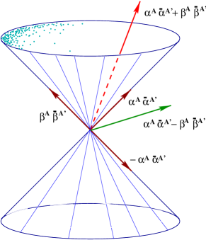
Figure 1: Causal structure of four-dimensional space-time. The canonical form of the spinor decomposition of the four-vector associated with a space-time interval determines its causal properties.

Here it is understood that in case (iii) the spinors $\alpha^{\bf A}$ and $\beta^{\bf A}$ do not coincide in direction. It is interesting to note that once the canonical form for $r^{{\bf AA}^{\prime}}$ is specified, then so is the causal relationship that it determines on space-time. This correspondence is illustrated in Figure 1. On the other hand, the specification of $r^{{\bf AA}^{\prime}}$ does not completely determine the spinors $\alpha^{\bf A}$ and $\beta^{\bf A}$. In general there is some freedom, and this is expressed by a group of transformations. In particular, if $r^{{\bf AA}^{\prime}}$ is null, then this freedom is the phase shift $\alpha^{\bf A}\to{{\rm e}}^{{\rm i}\theta}\alpha^{\bf A}$, and the relevant group is $U(1)$. If $r^{{\bf AA}^{\prime}}$ is time-like, then the group is $U(2)$, and if $r^{{\bf AA}^{\prime}}$ is space-like, the group is $U(1,1)$.

3 Hyperspin spaces

The terminology ‘hyperspinor’ is due to Finkelstein Finkelstein1 . Essentially the same concept (although introduced for different purposes) is also touched on in Hughston1 . The idea of a hyperspinor is a simple one—we replace the two-component spinors associated with four-dimensional space-time with $r$-component spinors. Thus we can regard hyperspin space as the vector space ${\mathbb{C}}^{r}$ with some extra structure. In particular, in addition to the original hyperspin space we have three other vector spaces—the dual hyperspin space, the complex conjugate hyperspin space, and the dual complex conjugate hyperspin space.

The theory of hyperspin has been pursued by a number of authors Borowiec1 ; Borowiec2 ; Brody2 ; Finkelstein2 ; Finkelstein3 ; Finkelstein4 ; Holm1 ; Holm2 ; Holm3 ; Holm4 ; Solovyov ; Urbantke , and the material we describe here builds on various aspects of this work. Let us write ${\mathbb{S}}^{A}$ and ${\mathbb{S}}^{A^{\prime}}$, respectively, for the complex $r$-dimensional vector spaces of unprimed and primed hyperspinors. For hyperspinors we use italic indices to distinguish them from the boldface indices used exclusively for two-component spinors. It is assumed that ${\mathbb{S}}^{A}$ and ${\mathbb{S}}^{A^{\prime}}$ are related by an anti-linear isomorphism under the operation of complex conjugation. Thus if $\alpha^{A}\in{\mathbb{S}}^{A}$, then under complex conjugation we have $\alpha^{A}\to{\bar{\alpha}}^{A^{\prime}}$, where ${\bar{\alpha}}^{A^{\prime}}\in{\mathbb{S}}^{A^{\prime}}$. The dual spaces associated with ${\mathbb{S}}^{A}$ and ${\mathbb{S}}^{A^{\prime}}$ are denoted ${\mathbb{S}}_{A}$ and ${\mathbb{S}}_{A^{\prime}}$, respectively. If $\alpha^{A}\in{\mathbb{S}}^{A}$ and $\beta_{A}\in{\mathbb{S}}_{A}$, then their inner product is denoted $\alpha^{A}\beta_{A}$. Likewise if $\gamma^{\,A^{\prime}}\in{\mathbb{S}}^{A^{\prime}}$ and $\delta_{A^{\prime}}\in{\mathbb{S}}_{A^{\prime}}$ then their inner product is $\gamma^{\,A^{\prime}}\delta_{A^{\prime}}$.

We also introduce the totally antisymmetric hyperspinors of rank $r$ associated with the spaces ${\mathbb{S}}^{A}$, ${\mathbb{S}}_{A}$, ${\mathbb{S}}^{A^{\prime}}$, and ${\mathbb{S}}_{A^{\prime}}$. These will be denoted $\varepsilon^{AB\cdots C}$, $\varepsilon_{AB\cdots C}$, $\varepsilon^{A^{\prime}B^{\prime}\cdots C^{\prime}}$, and $\varepsilon_{A^{\prime}B^{\prime}\cdots C^{\prime}}$, respectively. The choice of these antisymmetric hyperspinors is unique up to an overall scale factor. Once a choice has been made for $\varepsilon_{AB\cdots C}$, then the other epsilon hyperspinors are determined by the relations

$$\varepsilon^{AB\cdots C}\varepsilon_{AB\cdots C}=r!,\quad\varepsilon^{A^{\prime}B^{\prime}\cdots C^{\prime}}\varepsilon_{A^{\prime}B^{\prime}\cdots C^{\prime}}=r!,\quad{\rm and}\quad\varepsilon_{A^{\prime}B^{\prime}\cdots C^{\prime}}={\bar{\varepsilon}}_{A^{\prime}B^{\prime}\cdots C^{\prime}},$$ (19)

where ${\bar{\varepsilon}}_{A^{\prime}B^{\prime}\cdots C^{\prime}}$ is the complex conjugate of $\varepsilon_{AB\cdots C}$.

Now let $\Lambda^{m}=\Lambda^{A_{1}A_{2}\cdots A_{m}}$ denote the skew tensor product space ${\mathbb{S}}^{A_{1}}\wedge{\mathbb{S}}^{A_{2}}\wedge\cdots\wedge{\mathbb{S}}^{A_{m}}$. Using an analogous notation, we introduce the spaces $\Lambda_{m}$, $\Lambda^{m^{\prime}}$, and $\Lambda_{m^{\prime}}$ for each $m=0,1,\ldots,r$. Then once the epsilon hyperspinors have been fixed we have a collection of maps of the form

$$\varepsilon_{r}\!:\,\Lambda^{m}\to\Lambda_{r-m},\quad\!\varepsilon^{r}\!:\,\Lambda_{m}\to\Lambda^{r-m},\quad\!\varepsilon_{r^{\prime}}\!:\,\Lambda^{m^{\prime}}\to\Lambda_{r^{\prime}-m^{\prime}},\quad\!{\rm and}\quad\!\varepsilon^{r^{\prime}}\!:\,\Lambda_{m^{\prime}}\to\Lambda^{r^{\prime}-m^{\prime}}.$$

As a consequence, a wide range of algebraic theorems can be formulated, which are useful in calculations. For example, if $\alpha^{A}\beta_{A}=0$ then $\beta_{A}$ must be of the form

$$\beta_{A}=\varepsilon_{ABC\cdots D}\alpha^{B}\mu^{C\cdots D}$$ (20)

for some $\mu^{C\cdots D}\in\Lambda^{r-2}$.

4 Quantum space-time

Now we introduce the complex matrix space ${\mathbb{C}}^{AA^{\prime}}={\mathbb{S}}^{A}\otimes{\mathbb{S}}^{A^{\prime}}$. An element $x^{\,AA^{\prime}}\in{\mathbb{C}}^{AA^{\prime}}$ is said to be real if it satisfies the (weak) Hermitian property $x^{\,AA^{\prime}}={\bar{x}}^{A^{\prime}A}$, where ${\bar{x}}^{A^{\prime}A}$ is the complex conjugate of $x^{\,AA^{\prime}}$. We shall have more to say about weak versus strong Hermiticity conditions in relation to the idea of symmetry breaking. We denote the vector space of real elements of ${\mathbb{C}}^{AA^{\prime}}$ by ${\mathbb{R}}^{AA^{\prime}}$. The elements of ${\mathbb{R}}^{AA^{\prime}}$ constitute what we call the real quantum space-time ${\mathcal{H}}^{r^{2}}$ of dimension $r^{2}$. We then regard $\mathcal{C\!H}^{r^{2}}={\mathbb{C}}^{AA^{\prime}}$ as the complexification of ${\mathcal{H}}^{r^{2}}$. Many problems in ${\mathcal{H}}^{r^{2}}$ are best first approached as problems in $\mathcal{C\!H}^{r^{2}}$, and hence sometimes although we refer to ${\mathcal{H}}^{r^{2}}$ our operations are actually carried out in $\mathcal{C\!H}^{r^{2}}$.

Let $x^{\,AA^{\prime}}$ and $y^{\,AA^{\prime}}$ be points in ${\mathcal{H}}^{r^{2}}$, and write $r^{\,AA^{\prime}}=x^{\,AA^{\prime}}-y^{\,AA^{\prime}}$ for the corresponding separation vector, which is independent of the choice of origin. Using the index-clumping convention we set $x^{\rm a}=x^{\,AA^{\prime}}$, $y^{\rm a}=y^{\,AA^{\prime}}$, $r^{\rm a}=r^{\,AA^{\prime}}$, and for the separation of $x^{\rm a}$ and $y^{\rm a}$ in ${\mathcal{H}}^{r^{2}}$ we write $r^{\rm a}=x^{\rm a}-y^{\rm a}$. There is a natural causal structure induced on such intervals by the so-called ‘chronometric tensor’. Making use of the index-clumping convention, we define this fundamental tensor (introduced by Finkelstein Finkelstein1 ) by the following basic relation:

$$g_{{\rm ab\cdots c}}=\varepsilon_{AB\cdots C}\,\varepsilon_{A^{\prime}B^{\prime}\cdots C^{\prime}}.$$ (21)

The chronometric tensor, which is of rank $r$, is totally symmetric and is nondegenerate in the sense that for any vector $r^{\rm a}$ the condition $r^{\rm a}g_{\rm ab\cdots c}=0$ implies $r^{\rm a}=0$. We say that $x^{\rm a}$ and $y^{\rm a}$ in ${\mathcal{H}}^{r^{2}}$ have a ‘degenerate’ separation if the chronometric form

$$\Delta(r)=g_{{\rm ab\cdots c}}r^{\rm a}r^{\rm b}\cdots r^{\rm c}$$ (22)

vanishes for $r^{\rm a}=x^{\rm a}-y^{\rm a}$. Degenerate separation is equivalent to the vanishing of the determinant of the matrix $r^{\,AA^{\prime}}$, that is,

$$\varepsilon_{AB\cdots C}\,\varepsilon_{A^{\prime}B^{\prime}\cdots C^{\prime}}r^{\,AA^{\prime}}r^{\,BB^{\prime}}\cdots r^{\,CC^{\prime}}=0.$$ (23)

If the hyperspin space has dimension $r=2$, this reduces to the usual condition for $x^{\rm a}$ and $y^{\rm a}$ to be null-separated in Minkowski space. For $r>2$, however, the situation is more complicated since there are various degrees of degeneracy that can arise between two points of quantum space-time, of which ‘nullness’ (in the Minkowskian sense) is only the most extreme.

As an example, consider $r=3$. In this case the quantum space-time has dimension nine, and the chronometric form is given by

$$\Delta=g_{\rm abc}r^{\rm a}r^{\rm b}r^{\rm c}.$$ (24)

The different possibilities that can arise for the separation vector are as follows:

• $g_{\rm abc}r^{\rm c}=0$:

  $$\begin{array}[]{ll}r^{\,AA^{\prime}}=0&\textrm{zero separation}\end{array}$$ (26)

• $g_{\rm abc}r^{\rm b}r^{\rm c}=0$ and $g_{\rm abc}r^{\rm c}\neq 0$:

  $$\begin{array}[]{ll}r^{\,AA^{\prime}}=\alpha^{A}{\bar{\alpha}}^{A^{\prime}}&\textrm{future-pointing null separation}\\ r^{\,AA^{\prime}}=-\alpha^{A}{\bar{\alpha}}^{A^{\prime}}&\textrm{past-pointing null separation}\end{array}$$ (29)

• $\Delta=0$ and $g_{\rm abc}r^{\rm b}r^{\rm c}\neq 0$:

  $$\begin{array}[]{ll}r^{\,AA^{\prime}}=\alpha^{A}{\bar{\alpha}}^{A^{\prime}}+\beta^{A}{\bar{\beta}}^{A^{\prime}}&\textrm{degenerate time-like future-pointing separation}\\ r^{\,AA^{\prime}}=\alpha^{A}{\bar{\alpha}}^{A^{\prime}}-\beta^{A}{\bar{\beta}}^{A^{\prime}}&\textrm{degenerate space-like separation}\\ r^{\,AA^{\prime}}=-\alpha^{A}{\bar{\alpha}}^{A^{\prime}}-\beta^{A}{\bar{\beta}}^{A^{\prime}}&\textrm{degenerate time-like past-pointing separation}\end{array}$$ (33)

• $\Delta\neq 0$ and $g_{\rm ab}r^{\rm a}r^{\rm b}\neq 0$:

  $$\begin{array}[]{ll}r^{\,AA^{\prime}}=\alpha^{A}{\bar{\alpha}}^{A^{\prime}}+\beta^{A}{\bar{\beta}}^{A^{\prime}}+\gamma^{\,A}{\bar{\gamma}}^{\,A^{\prime}}&\textrm{future pointing time-like separation}\\ r^{\,AA^{\prime}}=\alpha^{A}{\bar{\alpha}}^{A^{\prime}}+\beta^{A}{\bar{\beta}}^{A^{\prime}}-\gamma^{\,A}{\bar{\gamma}}^{\,A^{\prime}}&\textrm{semi-space-like separation}\\ r^{\,AA^{\prime}}=\alpha^{A}{\bar{\alpha}}^{A^{\prime}}-\beta^{A}{\bar{\beta}}^{A^{\prime}}-\gamma^{\,A}{\bar{\gamma}}^{\,A^{\prime}}&\textrm{semi-space-like separation}\\ r^{\,AA^{\prime}}=-\alpha^{A}{\bar{\alpha}}^{A^{\prime}}-\beta^{A}{\bar{\beta}}^{A^{\prime}}-\gamma^{\,A}{\bar{\gamma}}^{\,A^{\prime}}&\textrm{past pointing time-like separation}\end{array}$$ (38)

When the separation of two points of quantum space-time is degenerate, we define the ‘degree’ of degeneracy by the rank of the matrix $r^{\,AA^{\prime}}$. Null separation is the case for which the degeneracy is of the first degree, i.e. where $r^{\,AA^{\prime}}$ is of rank one, and thus satisfies a system of quadratic relations of the following form:

$$\varepsilon_{AB\cdots C}\,\varepsilon_{A^{\prime}B^{\prime}\cdots C^{\prime}}r^{\,AA^{\prime}}r^{BB^{\prime}}=0,$$ (39)

or equivalently

$$g_{{\rm ab\cdots c}}r^{\rm a}r^{\rm b}=0.$$ (40)

This implies that $r^{\,AA^{\prime}}$ can be expressed in the ‘null’ form

$$r^{\,AA^{\prime}}=\pm\alpha^{A}{\bar{\alpha}}^{A^{\prime}}$$ (41)

for some $\alpha^{A}$. In the case of degeneracy of the second degree, $r^{\,AA^{\prime}}$ is of rank two and satisfies a set of cubic relations given by

$$\varepsilon_{ABC\cdots D}\,\varepsilon_{A^{\prime}B^{\prime}C^{\prime}\cdots D^{\prime}}r^{\,AA^{\prime}}r^{BB^{\prime}}r^{CC^{\prime}}=0,$$ (42)

or equivalently

$$g_{{\rm abc\cdots d}}r^{\rm a}r^{\rm b}r^{\rm c}=0.$$ (43)

In this situation $r^{\,AA^{\prime}}$ can be put into one of the following three canonical forms:

• $r^{\,AA^{\prime}}=\alpha^{A}{\bar{\alpha}}^{A^{\prime}}+\beta^{A}{\bar{\beta}}^{A^{\prime}}$,

• $r^{\,AA^{\prime}}=\alpha^{A}{\bar{\alpha}}^{A^{\prime}}-\beta^{A}{\bar{\beta}}^{A^{\prime}}$,

• $r^{\,AA^{\prime}}=-\alpha^{A}{\bar{\alpha}}^{A^{\prime}}-\beta^{A}{\bar{\beta}}^{A^{\prime}}$.

In case (a), $x^{\rm a}$ lies to the future of $y^{\rm a}$, and $r^{\rm a}$ can be thought of as a degenerate future-pointing time-like vector. In case (b), $r^{\rm a}$ can be thought of as a degenerate space-like separation. In case (c), $x^{\rm a}$ lies to the past of $y^{\rm a}$, and $r^{\rm a}$ is a degenerate past-pointing time-like vector. A similar analysis can be applied to degenerate separations of other ‘intermediate’ degrees.

If the determinant of the $r$-by-$r$ weakly Hermitian matrix $r^{\,AA^{\prime}}$ is nonvanishing, and $r^{\,AA^{\prime}}$ is thus of maximal rank, then the chronometric form $\Delta$ is nonvanishing. In that case the matrix $r^{\,AA^{\prime}}$ can be represented in the following canonical form:

$$r^{\,AA^{\prime}}=\pm\alpha^{A}{\bar{\alpha}}^{A^{\prime}}\pm\beta^{A}{\bar{\beta}}^{A^{\prime}}\pm\cdots\pm\gamma^{\,A}{\bar{\gamma}}^{\,A^{\prime}},$$ (44)

with the presence of $r$ nonvanishing terms, where the $r$ hyperspinors $\alpha^{A},\beta^{A},\cdots,\gamma^{\,A}$ are all linearly independent.

Let us write $(p,q)$ for the numbers of plus and minus signs appearing in the canonical form for the matrix $r^{\,AA^{\prime}}$ given above. We call $(p,q)$ the ‘signature’ of $r^{\,AA^{\prime}}$. The hyperspinors $\alpha^{A},\beta^{A},\cdots,\gamma^{\,A}$ are determined by the specification of $r^{\,AA^{\prime}}$ only up to an overall unitary (or pseudo-unitary) transformation of the form

$$\alpha^{A}_{n}\to U^{m}_{n}\alpha^{A}_{m},$$ (45)

where $n,m=1,2,\ldots,r$, and

$$\alpha^{A}_{n}=\{\alpha^{A},\beta^{A},\cdots,\gamma^{\,A}\}.$$ (46)

The signature $(p,q)$ is nevertheless an invariant of $r^{\,AA^{\prime}}$. In the cases for which the signature is $(r,0)$ or $(0,r)$ we say that $r^{\,AA^{\prime}}$ is future-pointing time-like or past-pointing time-like, respectively. Then recalling the definition (22) for the associated chronometric form, we define the ‘proper time interval’ between the events $x^{\rm a}$ and $y^{\rm a}$ by the formula

$$\|x-y\|=|\Delta|^{\frac{1}{r}}.$$ (47)

In the case $r=2$ we then recover the standard Minkowskian proper-time interval between the given events.

A remarkable feature of the causal structure of quantum space-time is that the essential physical features of the causal structure of Minkowski space are preserved. In particular, the space of future-pointing time-like vectors forms a convex cone. The same is true when we consider the structure of the associated momentum space, from which it follows that we can also give a good definition of what is meant by ‘positive energy’.

5 Equations of motion

Now suppose that $\lambda\mapsto x^{\,AA^{\prime}}(\lambda)$ defines a smooth curve $\gamma$ in ${\mathcal{H}}^{r^{2}}$ for $\lambda\in[a,b]\subset{\mathbb{R}}$. Then $\gamma$ will be said to be time-like if the tangent vector along $\gamma$,

$$v^{AA^{\prime}}(\lambda)=\frac{{\rm d}}{{\rm d}\lambda}x^{\,AA^{\prime}}(\lambda),$$ (48)

is time-like and future-pointing. In that case we define the proper time $s$ elapsed along $\gamma$ by the integral

$$s=\int_{a}^{b}\left[g_{{\rm ab}\cdots{\rm c}}v^{{\rm a}}v^{\rm b}\cdots v^{\rm c}\right]^{\frac{1}{r}}{\rm d}\lambda.$$ (49)

In the case of a very small interval, we can also write this in the ‘pseudo-Finslerian’ form

$$({\rm d}s)^{r}=g_{{\rm ab}\cdots{\rm c}}{\rm d}x^{\rm a}{\rm d}x^{\rm b}\cdots{\rm d}x^{\rm c}.$$ (50)

In the case $r=2$ this clearly reduces to the standard pseudo-Riemannian expression for the line element.

Now let us consider the condition $\gamma$ must satisfy in order to be a geodesic in ${\mathcal{H}}^{r^{2}}$. Since the geometry is not Riemannian, the answer may not be entirely obvious. In the case of a time-like curve, we can choose the proper time as the parameter along the curve, in which case the resulting affine parameterisation of the curve is determined up to transformations of the form $s\to s+k$ where $k$ is a constant. The equation of motion for the situation in which $\gamma$ is a time-like geodesic is obtained by an application of the calculus of variations to formula (49). As usual, we assume the variation vanishes at the endpoints. Writing

$$L=\left(g_{{\rm abc}\cdots{\rm d}}v^{\rm a}v^{\rm b}v^{\rm c}\cdots v^{\rm d}\right)^{\frac{1}{r}},$$ (51)

a standard argument shows that $x^{\rm a}(\lambda)$ describes a geodesic only if the velocity vector $v^{\rm a}$ satisfies the Euler-Lagrange equation

$$\frac{{\rm d}}{{\rm d}\lambda}\left(\frac{\partial L}{\partial v^{\rm a}}\right)=0.$$ (52)

A calculation shows that this condition is given more explicitly by

$$g_{{\rm abc}\cdots{\rm d}}\frac{{\rm d}v^{\rm b}}{{\rm d}\lambda}v^{\rm c}\cdots v^{\rm d}=\phi\,g_{{\rm abc}\cdots{\rm d}}v^{\rm b}v^{\rm c}\cdots v^{\rm d},$$ (53)

where

$$\phi=\frac{1}{L}\frac{{\rm d}L}{{\rm d}\lambda}.$$ (54)

If $\lambda$ is chosen to be proper time, then $\phi=0$ and the geodesic equation takes to form

$$g_{{\rm abc}\cdots{\rm d}}{\dot{v}}^{\rm b}v^{\rm c}\cdots v^{\rm d}=0,$$ (55)

where the dot denotes differentiation with respect to proper time.

In the case $r=2$ the geodesic equation (55) reduces to the familiar relation ${\dot{v}}^{\rm a}=0$. We shall now show that the geodesic equation also implies ${\dot{v}}^{\rm a}=0$ in the case of a general quantum space-time with $r>2$. It suffices to examine the case $r=3$, which will indicate the relevant line of argument. For $r=3$ the geodesic equation takes the form

$$g_{{\rm abc}}{\dot{v}}^{\rm b}v^{\rm c}=0,$$ (56)

which can be expressed in terms of hyperspinors in the form

$$\varepsilon_{ABC}\,\varepsilon_{A^{\prime}B^{\prime}C^{\prime}}\,{\dot{v}}^{BB^{\prime}}v^{CC^{\prime}}=0.$$ (57)

This relation can then be written

$${\dot{v}}^{BB^{\prime}}v^{CC^{\prime}}-{\dot{v}}^{CB^{\prime}}v^{BC^{\prime}}-{\dot{v}}^{BC^{\prime}}v^{CB^{\prime}}+{\dot{v}}^{CC^{\prime}}v^{BB^{\prime}}=0.$$ (58)

Because $\det(v^{AA^{\prime}})\neq 0$ we know that $v^{AA^{\prime}}$ has an inverse $u_{AA^{\prime}}$ satisfying

$$v^{AA^{\prime}}u_{BA^{\prime}}=\delta^{A}_{\ B}\quad{\rm and}\quad v^{AA^{\prime}}u_{AB^{\prime}}=\delta^{A^{\prime}}_{\ B^{\prime}}.$$ (59)

Therefore, contracting (58) with $u_{BB^{\prime}}$ we obtain

$$(u_{BB^{\prime}}{\dot{v}}^{BB^{\prime}})v^{CC^{\prime}}+(r-2){\dot{v}}^{CC^{\prime}}=0.$$ (60)

This equation shows that if ${\dot{v}}^{CC^{\prime}}$ were not zero, then it would have to be proportional to $v^{CC^{\prime}}$. However, if that were so, then

$$\varepsilon_{ABC}\,\varepsilon_{A^{\prime}B^{\prime}C^{\prime}}\,{\dot{v}}^{BB^{\prime}}v^{CC^{\prime}}=0$$ (61)

would imply $\det(v^{CC^{\prime}})=0$, contrary to the assumption that $v^{CC^{\prime}}$ is time-like. It follows that ${\dot{v}}^{\rm a}=0$. A similar argument shows that for all $r\geq 2$ the geodesic equation (55) implies ${\dot{v}}^{\rm a}=0$. Hence we have deduced the following result. Let $y^{\rm a}$ and $z^{\rm a}$ be quantum space-time points with the property that $y^{\rm a}-z^{\rm a}$ is time-like and future-pointing. Then the affinely parametrised geodesic $\gamma$ connecting these points in ${\mathcal{H}}^{r^{2}}$ is given by

$$X^{\rm a}(s)=z^{\rm a}+\frac{y^{\rm a}-z^{\rm a}}{[\Delta(y,z)]^{1/r}}\,s$$ (62)

for $s\in(-\infty,\infty)$, where

$$\Delta(y,z)=g_{\rm ab\cdots c}(y^{\rm a}-z^{\rm a})(y^{\rm b}-z^{\rm b})\cdots(y^{\rm c}-z^{\rm c}).$$ (63)

6 Conserved quantities

It is a straightforward exercise to verify that the chronometric form $\Delta$ for the separation between two points is invariant when the points of ${\mathcal{H}}^{r^{2}}$ are subjected to transformations of the following type:

$$x^{\,AA^{\prime}}\to\lambda^{A}_{B}{\bar{\lambda}}^{A^{\prime}}_{B^{\prime}}x^{BB^{\prime}}+\beta^{AA^{\prime}}.$$ (64)

Here $\beta^{AA^{\prime}}$ represents an arbitrary translation in quantum space-time, $\lambda^{A}_{B}$ is an element of $SL(r,{\mathbb{C}})$, and ${\bar{\lambda}}^{A^{\prime}}_{B^{\prime}}$ is the complex conjugate of $\lambda^{A}_{B}$. The relation of this group of transformations to the Poincaré group in the case $r=2$ should be apparent. Indeed, one of the attractive features of the extension of space-time geometry that we are putting forward here is that the hyper-Poincaré group allows such a description, which implies a wide range of intuitively plausible physical features.

More generally, we remark that the proper hyper-Poincaré group preserves the signature of any space-time interval, whether or not the interval is degenerate, and hence leaves the causal relations between events unchanged. We refer to a transformation of the form

$$r^{\rm a}\to L^{\rm a}_{\rm b}r^{\rm b}$$ (65)

as a ‘hyper-Lorentz transformation’ if

$$L^{\rm a}_{\rm b}=\lambda^{A}_{B}{\bar{\lambda}}^{A^{\prime}}_{B^{\prime}}$$ (66)

for some element $\lambda^{A}_{B}\in SL(r,{\mathbb{C}})$. In the case of Minkowski space ($r=2$) it is well known that a two-component spinor $\xi^{\bf A}$ can be represented by a complex null bivector

$$\Lambda^{\rm ab}=\xi^{\bf A}\xi^{\bf B}\varepsilon^{{\bf A}^{\prime}{\bf B}^{\prime}}.$$ (67)

Conversely, the bivector $\Lambda^{\rm ab}$ determines $\xi^{\bf A}$ up to the transformation

$$\xi^{\bf A}\to-\xi^{\bf A}.$$ (68)

This geometrical ambiguity is often referred to as the fundamental ‘two-valuedness’ of two-component spinors in relativity theory. In the case of a general quantum space-time of dimension $r^{2}$, a hyperspinor $\xi^{A}$ can be represented by a complex null $r$-vector (antisymmetric tensor of rank $r$) of the form

$$\Lambda^{\rm ab\cdots c}=\xi^{A}\xi^{B}\cdots\xi^{C}\varepsilon^{A^{\prime}B^{\prime}\cdots C^{\prime}}.$$ (69)

The $r$-vector $\Lambda^{\rm ab\cdots c}$ is ‘null’ in the sense that

$$g_{\rm ab\cdots c}\Lambda^{\rm ap\cdots q}\Lambda^{\rm br\cdots s}=0.$$ (70)

Then $\Lambda^{\rm ab\cdots c}$ determines $\xi^{A}$ up to transformations of the form

$$\xi^{A}\to{\rm e}^{2\pi{\rm i}k/r}\xi^{A},$$ (71)

where $k=1,2,\ldots,r-1$. Hence we can say that hyperspinors have a fundamental ‘$r$-valuedness’ (cf. Holm Holm4 ).

The real dimension of the hyper-Lorentz group is $2r^{2}-2$, and thus the real dimension of the hyper-Poincaré group is $3r^{2}-2$. We observe that the dimension of the hyper-Poincaré group grows linearly with the dimension of the quantum space-time itself, which is given by $r^{2}$. This can be contrasted with the dimension of the group arising if we endow ${\mathbb{R}}^{r^{2}}$ with a standard Lorentzian metric with signature $(1,r^{2}-1)$. In that case the associated pseudo-orthogonal group has real dimension $\frac{1}{2}r^{2}(r^{2}-1)$, which together with the translation group gives a total dimension of $\frac{1}{2}r^{2}(r^{2}+1)$. The parsimonious dimensionality of the hyper-Poincaré group arises from the fact that it preserves the system of causal relations holding between pairs of points in quantum space-time.

In a flat four-dimensional space-time the symmetries of the Poincaré group are associated with a ten-parameter family of Killing vectors. Thus, for $r=2$ we have the Minkowski metric (9), and the Poincaré group is generated by the ten-parameter family of vector fields $\xi^{\rm a}$ on ${\mathfrak{M}}^{4}$ satisfying

$${\mathcal{L}}_{\xi}g_{\rm ab}=0,$$ (72)

where ${\mathcal{L}}_{\xi}$ denotes the Lie derivative with respect to $\xi^{\rm a}$. For any vector field $\xi^{\rm a}$ and any symmetric tensor field $g_{\rm ab}$ we have

$${\mathcal{L}}_{\xi}g_{\rm ab}=\xi^{\rm c}\nabla_{\!\rm c}g_{\rm ab}+2g_{{\rm c}({\rm a}}\nabla_{\!{\rm b})}\xi^{\rm c}.$$ (73)

If $g_{\rm ab}$ is the metric and $\nabla_{\!\rm a}$ denotes the associated covariant derivative satisfying

$$\nabla_{\!\rm a}g_{\rm bc}=0,$$ (74)

we obtain the Killing equation

$$\nabla_{\!({\rm a}}\xi_{{\rm b})}=0,$$ (75)

where $\xi_{\rm a}=g_{\rm ab}\xi^{\rm b}$. The condition ${\mathcal{L}}_{\xi}g_{\rm ab}=0$ therefore implies that $\xi^{\rm a}$ is a Killing vector.

For $r>2$ we have no Riemannian metric, and the usual relations between symmetries and Killing vectors are lost. What survives, however, is of interest. Specifically, to generate a symmetry of the quantum space-time the vector field $\xi^{\rm a}$ has to satisfy

$${\mathcal{L}}_{\xi}g_{\rm ab\cdots c}=0,$$ (76)

where $g_{\rm ab\cdots c}$ is the chronometric tensor. For a general vector field $\xi^{\rm a}$ and a general symmetric tensor field $g_{\rm ab\cdots c}$ we have

$${\mathcal{L}}_{\xi}g_{\rm ab\cdots c}=\xi^{\rm d}\nabla_{\!\rm d}g_{\rm ab\cdots c}+r\,g_{{\rm d}({\rm a\cdots b}}\nabla_{\!{\rm c})}\xi^{\rm d}.$$ (77)

In the case of the quantum space-time ${\mathcal{H}}^{r^{2}}$ we let $\nabla_{\!{\rm a}}$ be the natural flat connection for which

$$\nabla_{\!{\rm a}}g_{\rm bc\cdots d}=0.$$ (78)

Then to generate a symmetry of the chronometric structure of ${\mathcal{H}}^{r^{2}}$ the vector field $\xi^{\rm a}$ has to satisfy

$$g_{{\rm d}({\rm a\cdots b}}\nabla_{\!{\rm c})}\xi^{\rm d}=0.$$ (79)

Equation (79) can be written in an alternative form if we define a symmetric tensor $K_{\rm ab\cdots c}$ of rank $r-1$ by setting

$$K_{\rm ab\cdots c}=g_{\rm ab\cdots cd}\xi^{\rm d}.$$ (80)

Then (79) says that $K_{\rm ab\cdots c}$ satisfies the conditions for a symmetric Killing tensor:

$$\nabla_{\!({\rm a}}K_{\rm bc\cdots d)}=0.$$ (81)

Thus we see that ${\mathcal{H}}^{r^{2}}$ provides an example of a symmetry group generated by a family of Killing tensors. The symmetries of the quantum space-time are generated, more specifically, by a system of $3r^{2}-2$ irreducible symmetric Killing tensors of rank $r-1$. The significance of Killing tensors is that they are associated with conserved quantities. For other examples of Killing tensors arising in a physical context, see, e.g., Hughston8 ; Hughston9 ; Hughston10 ; Penrose9 ; Walker . In the present setting it follows that if the vector field $v^{\rm a}$ satisfies the geodesic equation, which on a quantum space-time of dimension $r^{2}$ is given, as we have seen, by

$$g_{\rm abc\cdots d}\left(v^{\rm e}\nabla_{\!\rm e}v^{\rm b}\right)v^{\rm c}\cdots v^{\rm d}=0,$$ (82)

and if $K_{\rm ab\cdots c}$ is the Killing tensor of rank $r-1$ given by (80), then we have the following conservation law:

$$v^{\rm e}\nabla_{\!\rm e}\left(K_{\rm ab\cdots c}v^{\rm a}v^{\rm b}\cdots v^{\rm c}\right)=0.$$ (83)

In other words, the quantity

$$K=K_{\rm ab\cdots c}v^{\rm a}v^{\rm b}\cdots v^{\rm c}$$ (84)

is a constant of the motion.

7 Hyper-relativistic mechanics

It follows from the material of the previous section that in higher-dimensional quantum space-times the main conservation laws and symmetry principles of relativistic physics remain intact. In particular, the conservation of hyper-relativistic momentum and angular momentum for a system of interacting particles can be given a well-defined formulation, the basic principles of which are similar to those applicable in the Minkowskian case.

For this purpose it will be useful to introduce the notion of an ‘elementary system’ in hyper-relativistic mechanics. Such a system is defined by its hyper-relativistic momentum and angular momentum. The hyper-relativistic momentum of an elementary system is given by a momentum covector $P_{\rm a}$. The associated mass $m$ is given (cf. Finkelstein1 ) by the following natural expression:

$$m=\left(g^{\rm ab\cdots c}P_{\rm a}P_{\rm b}\cdots P_{\rm c}\right)^{\frac{1}{r}}.$$ (85)

The hyper-relativistic angular momentum of an elementary system is given by a tensor $L^{\rm b}_{\rm a}$ of the form

$$L^{\rm b}_{\rm a}=l^{B}_{A}\delta^{B^{\prime}}_{A^{\prime}}+{\bar{l}}^{B^{\prime}}_{A^{\prime}}\delta^{B}_{A},$$ (86)

where the hyperspinor $l^{B}_{A}$ is required to be trace-free: $l^{A}_{A}=0$. The angular momentum is defined with respect to a choice of origin in such a manner that under a change of origin defined by a shift vector $\beta^{\rm a}$ we have

$$l^{B}_{A}\to l^{B}_{A}+P_{AC^{\prime}}\beta^{BC^{\prime}}.$$ (87)

In the case $r=2$ these formulae reduce to the usual expressions for relativistic momentum and angular momentum in a Minkowskian setting. The real covector

$$S_{AA^{\prime}}={\rm i}m^{-1}\left(l^{B}_{A}P_{A^{\prime}B}-{\bar{l}}^{B^{\prime}}_{A^{\prime}}P_{AB^{\prime}}\right)$$ (88)

is invariant under a change of origin, and carries the interpretation of the intrinsic spin of the elementary system. The magnitude of the spin is then defined by

$$S=|g^{\rm ab\cdots c}S_{\rm a}S_{\rm b}\cdots S_{\rm c}|^{\frac{1}{r}}.$$ (89)

In the case of a set of interacting hyper-relativistic systems we require that the total momentum and angular momentum should be conserved. This then implies conservation of the total mass and spin. In short, we see that the idea of ‘relativistic mechanics’ carries through nicely to the case of a general quantum space-time.

Now what is the interpretation of these conservation laws? We shall show later, once we introduce the idea of symmetry breaking, that hypermomentum can be interpreted as the momentum operator for a relativistic quantum system. Conservation of hypermomentum then can be thought of as conservation of four-momentum in relativistic quantum mechanics in the Heisenberg representation.

8 Complex null directions

In four-dimensional space-time it is useful in many contexts to examine the geometry of the space of complex null vectors at a point in the space-time. This has the effect of giving us a vivid picture of the local causal relationships in space-time, and by sticking with a complex picture we also retain the link with quantum mechanics. Thus we consider complex vectors $z^{\rm a}$ satisfying the quadratic equation

$$g_{\rm ab}z^{\rm a}z^{\rm b}=0.$$ (90)

In spinor terms this relation implies that the corresponding complex matrix $z^{{\bf AA}^{\prime}}$ is of the special form

$$z^{{\bf AA}^{\prime}}=\alpha^{\bf A}\beta^{{\bf A}^{\prime}}.$$ (91)

The space of complex vectors at a point in Minkowski space is ${\mathbb{C}}^{4}$. The space of complex directions (which results if we consider equivalence class of vectors modulo overall proportionality) is the complex projective 3-space ${\mathbb{P}}^{3}$. The null directions constitute a quadric ${\mathbb{Q}}^{2}$ in that space, which owing to the decomposition (91) has the structure of a doubly ruled surface

$${\mathbb{Q}}^{2}={\mathbb{P}}^{1}\times{\mathbb{P}}^{1}.$$ (92)

We can identify the first set of lines (the $\alpha$-lines) with the projective unprimed spinors, and the second set of lines (the $\beta$-lines) with the projective primed spinors. The quadric ${\mathbb{Q}}^{2}$ is ruled in such a way that two lines of the same type do not intersect, whereas two lines of the opposite type intersect at a point in ${\mathbb{Q}}^{2}$ (see Figure 2). This point corresponds to the null direction they jointly determine.

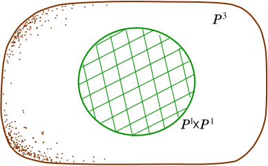
Figure 2: Complex null directions in a four-dimensional space-time. The space of directions at a point in complex Minkowski space has the geometry of a complex projective 3-space. The complex null directions constitute a quadric which has the structure of a doubly ruled surface ${\mathbb{P}}^{1}\times{\mathbb{P}}^{1}$.

In the case of a general quantum space-time of dimension $r^{2}$, we consider the space of complex vectors at a point, and examine the corresponding space of directions, which has the structure of a complex projective space ${\mathbb{P}}^{r^{2}-1}$. The space of degenerate complex directions, which is given by the vanishing of the chronometric form $g_{\rm ab\cdots c}z^{\rm a}z^{\rm b}\cdots z^{\rm c}$, is a hypersurface in ${\mathbb{P}}^{r^{2}-1}$, which we shall call ${\mathcal{D}}^{r^{2}-2}$.

The points of ${\mathcal{D}}^{r^{2}-2}$ correspond to degenerate directions of degree $r-1$. The null directions in ${\mathcal{D}}^{r^{2}-2}$ correspond to those directions for which the associated degenerate vectors are of minimal rank and hence of the form $z^{AA^{\prime}}=\alpha^{A}\beta^{A^{\prime}}$. These constitute a subvariety ${\mathbb{Q}}^{2r-2}\subset{\mathcal{D}}^{r^{2}-2}$ defined by the mutual intersection of a system of quadrics, given by the equation

$$g_{\rm ab\cdots c}z^{\rm a}z^{\rm b}=0.$$ (93)

In this situation we have

$${\mathbb{Q}}^{2r-2}={\mathbb{P}}^{r-1}\times{\mathbb{P}}^{r-1},$$ (94)

and we can identify the two systems of $(r-1)$-planes by which ${\mathbb{Q}}^{2r-2}$ is foliated, which we refer to as $\alpha$-planes and $\beta$-planes, as the spaces of projective unprimed and primed hyperspinors, respectively. The various degenerate directions of intermediate degree correspond to points in ${\mathcal{D}}^{r^{2}-2}$ lying on the linear spaces spanned by the joins of $d$ points in ${\mathbb{Q}}^{2r-2}$ ($d=2,3,\ldots,r$). The degree of degeneracy is given by the integer $d$.

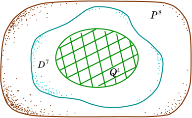
Figure 3: The space of complex null directions at a point in a quantum space-time of dimension nine. In this case the space of degenerate directions is given by a cubic surface ${\mathcal{D}}^{7}$ in the complex projective space ${\mathbb{P}}^{8}$. The complex null directions then constitute a four-dimensional doubly foliated subvariety ${\mathbb{Q}}^{4}={\mathbb{P}}^{2}\times{\mathbb{P}}^{2}$ in ${\mathcal{D}}^{7}$.

In the case $r=3$, illustrated in Figure 3, the space of complex directions at a point in $\mathcal{C\!H}^{9}$ is ${\mathbb{P}}^{8}$, and the degenerate directions constitute a cubic hypersurface ${\mathcal{D}}^{7}\subset{\mathbb{P}}^{8}$. The null directions lie in the doubly foliated surface

$${\mathbb{Q}}^{4}={\mathbb{P}}^{2}\times{\mathbb{P}}^{2}$$ (95)

in ${\mathcal{D}}^{7}$. The points of ${\mathcal{D}}^{7}$ all lie on the ‘first join’ of ${\mathbb{Q}}^{4}$ with itself; in other words, any point of ${\mathcal{D}}^{7}$ lies on a line joining two points of ${\mathbb{Q}}^{4}$. Thus we write ${\mathcal{D}}^{7}=J_{1}({\mathbb{Q}}^{4})$. The space ${\mathcal{D}}^{7}\!\setminus\!{\mathbb{Q}}^{4}$ then consists of degenerate directions that are strictly of the second degree. Note that any point of ${\mathbb{P}}^{8}$ can be represented as the join of three points in ${\mathbb{Q}}^{4}$, and hence $J_{2}({\mathbb{Q}}^{4})={\mathbb{P}}^{8}$.

In the case $r=4$, illustrated in Figure 4, the space of complex directions at a point in $\mathcal{C\!H}^{16}$ is the complex projective space ${\mathbb{P}}^{15}$, and the degenerate directions constitute a quartic hypersurface ${\mathcal{D}}^{14}\subset{\mathbb{P}}^{15}$. The null directions (degenerate direction of the first degree) lie on the doubly foliated surface

$${\mathcal{D}}_{(1)}={\mathbb{P}}^{3}\times{\mathbb{P}}^{3}$$ (96)

in ${\mathcal{D}}^{14}$. The degenerate directions of the second degree lie on the first join of ${\mathbb{Q}}^{6}$ with itself:

$${\mathcal{D}}_{(2)}=J_{1}({\mathbb{Q}}^{6}).$$ (97)

The degenerate directions of the third degree lie in

$${\mathcal{D}}_{(3)}=J_{2}({\mathbb{Q}}^{6})$$ (98)

and constitute the general elements of ${\mathcal{D}}^{14}$.

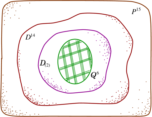
Figure 4: The space of complex null directions at a point in the quantum space-time ${\mathcal{H}}^{16}$. The degenerate directions of degree three constitute a quartic hypersurface ${\mathcal{D}}^{14}$ in ${\mathbb{P}}^{15}$. The null directions belong to a six-dimensional doubly foliated subvariety ${\mathbb{Q}}^{6}={\mathbb{P}}^{3}\times{\mathbb{P}}^{3}$. Degenerate directions of degree two constitute a submanifold ${\mathcal{D}}_{(2)}=J_{1}({\mathbb{Q}}^{6})\subset{\mathcal{D}}^{14}$ consisting of points that lie on lines spanned by pairs of points in the subvariety ${\mathbb{Q}}^{6}$.

9 Twistors and hypertwistors

The proceeding discussion of complex null directions can be seen as a ‘warm-up’ exercise for the introduction of the concept of hypertwistors. For this purpose we introduce a notation that closely parallels the standard notation for $r=2$ Penrose twistors. Let us denote by ${\mathbb{T}}^{\boldsymbol{\alpha}}$ the complex vector space of dimension $2r$ given by the pair $({\mathbb{S}}^{A},{\mathbb{S}}_{A^{\prime}})$. We write

$$Z^{\alpha}=(\omega^{A},\pi_{A^{\prime}})$$ (99)

for a typical element of ${\mathbb{T}}^{{\alpha}}$. Such elements will be referred to as ‘hypertwistors’ (also called ‘generalised twistors’ Eastwood ; Hughston1 ). Let ${\mathbb{T}}_{{\alpha}}=({\mathbb{S}}_{A},{\mathbb{S}}^{A^{\prime}})$ denote the space of dual hypertwistors. A natural pseudo-Hermitian structure can be introduced on the geometry of hypertwistors by means of the complex conjugation operation that maps $(\omega^{A},\pi_{A^{\prime}})\in{\mathbb{T}}^{{\alpha}}$ to $({\bar{\pi}}_{A},{\bar{\omega}}^{A^{\prime}})\in{\mathbb{T}}_{{\alpha}}$. The corresponding pseudo-Hermitian form is then given by

$$Z^{{\alpha}}{\bar{Z}}_{{\alpha}}=\omega^{A}{\bar{\pi}}_{A}+\pi_{A^{\prime}}{\bar{\omega}}^{A^{\prime}}.$$ (100)

It is straightforward to verify that the inner product $Z^{\alpha}{\bar{Z}}_{{\alpha}}$ is invariant under the action of the group $U(r,r)$. In the case $r=2$, the elements of ${\mathbb{T}}^{\boldsymbol{\alpha}}$ are standard Penrose twistors, and the relevant symmetry group is $U(2,2)$.

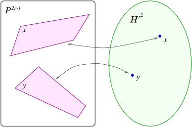
Figure 5: The Klein representation for a general quantum space-time. The aggregate consisting of all $(r-1)$-planes in the complex projective space ${\mathbb{P}}^{2r-1}$ forms a manifold of dimension $r^{2}$. This space is the complexified, compactified version of the quantum space-time ${\mathcal{C}}\!{\mathcal{H}}^{r^{2}}$.

The space ${\mathbb{P}}^{2r-1}$ of projective hypertwistors is a good starting point for the analysis of the conformal geometry of complex quantum space-time, which can be regarded as the Grassmannian variety of projective $(r-1)$-planes in ${\mathbb{P}}^{2r-1}$, as illustrated in Figure 5. More precisely, the aggregate of all projective $(r-1)$-planes in ${\mathbb{P}}^{2r-1}$ constitutes a compact manifold of dimension $r^{2}$, which we identify as the complexified, compactified quantum space-time ${\mathcal{C}}\!\bar{\mathcal{H}}^{r^{2}}$. The ‘finite’ points of ${\mathcal{C}}\!\bar{\mathcal{H}}^{r^{2}}$ correspond to those $(r-1)$-planes of ${\mathbb{P}}^{2r-1}$ that are determined by a linear relation of the form

$$\omega^{A}={\rm i}x^{\,AA^{\prime}}\pi_{A^{\prime}}$$ (101)

for some fixed $x^{\,AA^{\prime}}$. Thus for each (complex) point $x^{\,AA^{\prime}}$ in $\mathcal{C\!H}^{r^{2}}$ we obtain, according to equation (101), an $(r-1)$-plane in ${\mathbb{P}}^{2r-1}$. The aggregate of such $(r-1)$-planes constitute the points of $\mathcal{C\!H}^{r^{2}}$. The $(r-1)$-planes for which $x^{\,AA^{\prime}}$ is Hermitian then constitute the points of the real quantum space-time ${\mathcal{H}}^{r^{2}}$.

The conformal structure of a quantum space-time is implicit in the various possibilities arising for the intersections of $(r-1)$-planes in the projective hypertwistor space ${\mathbb{P}}^{2r-1}$. In the case $r=2$ (Penrose twistors) the projective space ${\mathbb{P}}^{3}$ contains a four-dimensional family of complex projective lines, the aggregation of which constitutes the associated space-time (see Figure 6). In this case, a pair of space-time points $x$ and $y$ are null-separated in the Minkowskian sense if and only if the corresponding lines in ${\mathbb{P}}^{3}$ intersect. The space of all complex projective lines in ${\mathbb{P}}^{3}$ constitutes a four-dimensional quadric hypersurface $Q^{4}$ in ${\mathbb{P}}^{5}$, which we identify as complexified, compactified Minkowski space-time ${\mathcal{C}}\!\bar{\mathcal{H}}^{4}$. The quadric $Q^{4}$ contains two systems of projective 2-planes, called $\alpha$-planes and $\beta$-planes. The $\alpha$-planes are in one-to-one correspondence with the points of ${\mathbb{P}}^{3}$, whereas the $\beta$-planes are in one-to-one correspondence with the 2-planes of ${\mathbb{P}}^{3}$, as illustrated in Figure 7.

The case $r=3$ has been studied closely by Finkelstein Finkelstein1 and his collaborators. In this case, the nine-dimensional quantum space-time ${\mathcal{C}}\!\bar{\mathcal{H}}^{9}$ arises when we consider the Grassmanian of complex projective 2-planes in complex projective 5-space. A pair of planes in ${\mathbb{P}}^{3}$ in general will not intersect. If they do, however, then there are three possibilities: they can intersect in a point, a line, or a plane. These situations correspond to the various levels of degeneracy obtainable for the separation vector. In particular, if the two planes intersect in a line, then the separation vector is null (see Figure 8).

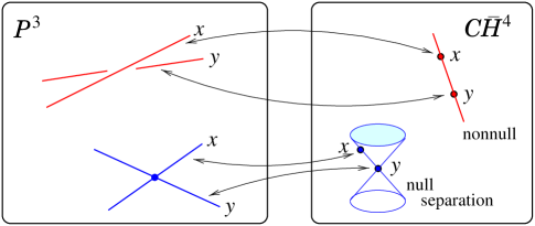
Figure 6: Twistor theory. The lines of the complex projective space ${\mathbb{P}}^{3}$ correspond to the points of the complex space-time ${\mathcal{C}}\!{\bar{\mathcal{H}}}^{4}$. Two points in ${\mathcal{C}}\!\bar{\mathcal{H}}^{4}$ are null-separated if and only if the corresponding lines in ${\mathbb{P}}^{3}$ intersect.

A pair of $(r-1)$-planes in ${\mathbb{P}}^{2r-1}$ will not in general intersect. This generic non-intersection property corresponds to the nonvanishing of the chronometric form for the separation vector of generic quantum space-time points. An $(r-1)$-plane in ${\mathbb{P}}^{2r-1}$ is represented by a simple skew hypertwistor $P^{{\alpha}{\beta}\cdots{\gamma}}$ of rank $r$. By a ‘simple’ skew hypertwistor we mean one of the form

$$P^{{\alpha}{\beta}\cdots{\gamma}}=A^{[{\alpha}}B^{{\beta}}\cdots C^{{\gamma}]}$$ (102)

for some set $A^{\alpha},B^{\alpha},\cdots,C^{\alpha}$ of $r$ hypertwistors. Suppose that the simple skew hypertwistors $P^{{\alpha}{\beta}\cdots{\gamma}}$ and $Q^{{\alpha}{\beta}\cdots{\gamma}}$ represent, respectively, the $(r-1)$-planes $P$ and $Q$ in ${\mathbb{P}}^{2r-1}$. A necessary and sufficient condition for the vanishing of the chronometric form for the corresponding space-time points is

$$\varepsilon_{\alpha\beta\cdots\gamma\rho\sigma\cdots\tau}P^{\alpha\beta\cdots\gamma}Q^{\rho\sigma\cdots\tau}=0,$$ (103)

where $\varepsilon_{{\alpha}{\beta}\cdots{\gamma}{\rho}{\sigma}\cdots{\tau}}$ is the skew hypertwistor of rank $2r$. We note that (103) is symmetric under the interchange of $P$ and $Q$ if $r$ is even, and antisymmetric if $r$ is odd. The vanishing of (103) is the condition that the planes $P$ and $Q$ contain a point in common. This means that the skew hypertwistors $P^{{\alpha}{\beta}\cdots{\gamma}}$ and $Q^{{\rho}{\sigma}\cdots{\tau}}$ contain at least one hypertwistor as a common factor. Thus, a necessary and sufficient condition for a pair of quantum space-time points to have a degenerate separation is that the corresponding $(r-1)$-planes in ${\mathbb{P}}^{2r-1}$ should intersect.

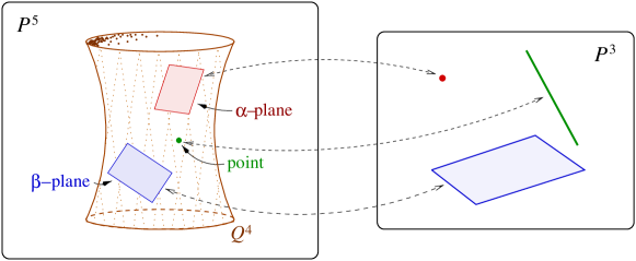
Figure 7: Complexified, compactified Minkowski space-time as the Klein quadric in complex projective 5-space. The aggregate of complex projective lines in ${\mathbb{P}}^{3}$ constitutes a nondegenerate quadric $Q^{4}$ in ${\mathbb{P}}^{5}$. The quadric contains two distinct systems of projective 2-planes, called $\alpha$-planes and $\beta$-planes. Any two distinct planes of the same type in $Q^{4}$ intersect at a point. Two planes of the opposite type in $Q^{4}$ will in general not intersect, but if they do, they intersect in a line. The points of ${\mathbb{P}}^{3}$ correspond to $\alpha$-planes in $Q^{4}$, and the 2-planes of ${\mathbb{P}}^{3}$ correspond to $\beta$-planes in $Q^{4}$.

More generally, the degeneracy $d$ of the separation of a pair of quantum space-time events is given by $d=r-m-1$, where $m$ is the dimensionality of the intersection of the corresponding $(r-1)$-planes in ${\mathbb{P}}^{2r-1}$. The possible degrees of degeneracy are $d=1,2,\ldots,r-1$. If we interpret the case of no intersection as an intersection of dimension $-1$, then a nondegenerate separation can be interpreted as a ‘degeneracy of degree $r$’. Thus separations of degree less than $r$ are degenerate, whereas a separation of degree $r$ is nondegenerate. The degree of degeneracy is given by the rank of the separation matrix $r^{\,AA^{\prime}}=x^{\,AA^{\prime}}-y^{\,AA^{\prime}}$.

Alternatively, given two skew hypertwistors $P^{{\alpha}{\beta}\cdots{\gamma}}$ and $Q^{{\alpha}{\beta}\cdots{\gamma}}$, each with $r$ indices, let us form the dual hypertwistor by

$$Q_{{\alpha}{\beta}\cdots{\gamma}}=\varepsilon_{{\alpha}{\beta}\cdots{\gamma}{\rho}{\sigma}\cdots{\tau}}Q^{{\rho}{\sigma}\cdots{\tau}}.$$ (104)

Then $d$ is the maximum number of index contractions we can make between $P^{{\alpha}{\beta}\cdots{\gamma}}$ and $Q_{{\alpha}{\beta}\cdots{\gamma}}$ without obtaining the result zero. If a single index contraction gives zero, this corresponds to the case where $P^{{\alpha}{\beta}\cdots{\gamma}}$ is proportional to $Q^{{\alpha}{\beta}\cdots{\gamma}}$. Thus $d=0$ (separation of degree zero) can be interpreted as the ‘completely degenerate’ case where the two space-time points coincide.

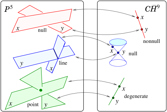
Figure 8: Hypertwistor theory for $r=3$. The aggregate of complex projective $2$-planes in ${\mathbb{P}}^{5}$ constitutes a nine-dimensional quantum space-time ${\mathcal{C}}\!{\bar{\mathcal{H}}}^{9}$. In general, two such planes will not intersect. If two planes intersect in a point, then the separation vector of the corresponding space-time points is degenerate. If the intersection is in a line, then the corresponding points are null-separated.

10 Hypertwistor fields

Now we present a few elementary applications of hypertwistor theory. In the case of a four-dimensional space-time, it is well known that twistors can be characterised as solutions of the differential equation

$$\nabla^{{\bf A}^{\prime}({\bf A}}\xi^{{\bf B})}=0,$$ (105)

the so-called ‘twistor equation’. Indeed, the solution of this equation is

$$\xi^{\bf A}=\omega^{\bf A}-{\rm i}x^{{\bf AA}^{\prime}}\pi_{{\bf A}^{\prime}},$$ (106)

and the associated twistor is determined by the fixed spinor pair $(\omega^{\bf A},\pi_{{\bf A}^{\prime}})$. More generally, in the case of a quantum space-time of dimension $r^{2}$ we consider the equation

$$r\nabla_{AA^{\prime}}\xi^{C}=\delta^{C}_{A}\nabla_{DA^{\prime}}\xi^{D}.$$ (107)

It is not difficult to verify that in the case $r=2$ equation (107) reduces to the conventional twistor equation (105). The solutions of (107) can be expressed in terms of generalised twistors:

$$\xi^{A}=\omega^{A}-{\rm i}x^{\,AA^{\prime}}\pi_{A^{\prime}},$$ (108)

where $\omega^{A}$ and $\pi_{A^{\prime}}$ are constant. This result is established in Hughston1 .

We note that a necessary and sufficient condition for a hypertwistor field $\xi^{A}(x)$ to satisfy the hypertwistor equation (107) is that it should satisfy

$$\sigma_{C}\sigma_{[A}\nabla_{B]C^{\prime}}\xi^{C}=0$$ (109)

for all values of $\sigma_{A}$. For $r=2$ the twistor equation (105) is a special case of a more general nonlinear partial differential equation known as the geodesic shear-free condition:

$$\xi^{\bf A}\xi^{\bf B}\nabla_{{\bf A}^{\prime}{\bf A}}\xi_{\bf B}=0.$$ (110)

When $r>2$, however, the connection between the twistor equation and the geodesic shear-free condition is lost, and the appropriate generalisation of the latter is

$$\left(\xi_{[A}\nabla_{B]B^{\prime}}\xi_{[C}\right)\xi_{D]}=0,$$ (111)

which reduces to the geodesic shear-free condition (110) when $r=2$. Solutions of the equation (111) can be generated through the consideration of the intersections of projective $(r-1)$-planes in ${\mathbb{P}}^{2r-1}$ with certain types of complex analytic varieties in ${\mathbb{P}}^{2r-1}$.

Now let us consider the dynamical equations for fields of totally null momentum on a general quantum space-time. The relevant field equations take the form

$$\nabla_{A[A^{\prime}}\nabla_{B^{\prime}]B}\phi=0,$$ (112)

$$\nabla_{A[A^{\prime}}\phi_{B^{\prime}]\cdots C^{\prime}}=0,$$ (113)

and

$$\nabla_{A^{\prime}[A}\phi_{B]\cdots C}=0.$$ (114)

These equations generalise the zero rest-mass equations for each helicity $s=\pm\frac{1}{2}n$ (where $n=0,1,2,\ldots$) in four-dimensional space-time.

The solutions can be described briefly as follows. We write $Z^{\alpha}=(\omega^{A},\pi_{A^{\prime}})$ and let $\psi(Z^{\alpha})$ denote an analytic, homogeneous function of degree $-r+2s$ defined on some region of the hypertwistor space. For $s=0$ we set

$$\phi(x)=\oint\psi({\rm i}x^{\,AA^{\prime}}\pi_{A^{\prime}},\pi_{A^{\prime}})\vartriangle\!\!\pi,$$ (115)

where the differential form $\vartriangle\!\!\pi$ is given by

$$\vartriangle\!\!\pi=\epsilon^{A^{\prime}B^{\prime}\cdots C^{\prime}}\pi_{A^{\prime}}\pi_{B^{\prime}}\cdots\pi_{C^{\prime}}.$$ (116)

Note that $\vartriangle\!\!\pi$ is homogeneous of degree $r$ in $\pi_{A^{\prime}}$, and thus that the quantity appearing in the integral sign in (115) is homogeneous of degree zero. Similarly, for helicity $s=-\frac{1}{2}$ we define

$$\phi_{A^{\prime}}(x)=\oint\pi_{A^{\prime}}\psi({\rm i}x^{\,AA^{\prime}}\pi_{A^{\prime}},\pi_{A^{\prime}})\vartriangle\!\!\pi,$$ (117)

and for helicity $s=\frac{1}{2}$ we define

$$\phi_{A^{\prime}}(x)=\oint\frac{\partial}{\partial\omega^{A}}\psi({\rm i}x^{\,AA^{\prime}}\pi_{A^{\prime}},\pi_{A^{\prime}})\vartriangle\!\!\pi.$$ (118)

Here it is understood that first we differentiate $\psi(\omega^{A},\pi_{A^{\prime}})$ with respect to $\omega^{A}$, and we set $\omega^{A}={\rm i}x^{\,AA^{\prime}}\pi_{A^{\prime}}$ before integrating. A proposition established in Hughston1 shows that the contour integrals (115), (117), and (118) satisfy the totally null momentum conditions (112), (113), and (114), respectively.

As an illustration, let us first take the simplest case, given by equation (115) for $r=3$. For our hypertwistor function we take

$$\psi(Z^{\alpha})=\frac{1}{P_{\alpha}Z^{\alpha}Q_{\beta}Z^{\beta}R_{\gamma}Z^{\gamma}},$$ (119)

where $P_{\alpha}$, $Q_{\beta}$, and $R_{\gamma}$ denote fixed points in the dual hypertwistor space. For their hyperspinor decomposition we write

$$P_{\alpha}=(p_{A},p^{\,A^{\prime}}),\quad Q_{\alpha}=(q_{A},q^{\,A^{\prime}}),\quad{\rm and}\quad R_{\alpha}=(r_{A},r^{\,A^{\prime}}),$$ (120)

and set

$${\tilde{p}}^{\,A^{\prime}}(x)=p^{\,A^{\prime}}+{{\rm i}}x^{\,A^{\prime}A}p_{A},\quad{\tilde{q}}^{\,A^{\prime}}(x)=q^{\,A^{\prime}}+{{\rm i}}x^{\,A^{\prime}A}q_{A},\quad{\rm and}\quad{\tilde{r}}^{\,A^{\prime}}(x)=r^{\,A^{\prime}}+{{\rm i}}x^{\,A^{\prime}A}r_{A},$$ (121)

where ${\tilde{p}}^{\,A^{\prime}}$, ${\tilde{q}}^{\,B^{\prime}}$, and ${\tilde{r}}^{\,C^{\prime}}$ are solutions of the primed analogue

$$r\nabla_{AA^{\prime}}{\tilde{\eta}}^{C^{\prime}}=\delta^{C^{\prime}}_{A^{\prime}}\nabla_{AD^{\prime}}{\tilde{\eta}}^{D^{\prime}},$$ (122)

of the hypertwistor equation (107). Inserting this expression into the contour integral formula, we obtain the result

$$\phi(x)=\frac{4\pi^{2}}{\varepsilon_{A^{\prime}B^{\prime}C^{\prime}}{\tilde{p}}^{\,A^{\prime}}{\tilde{q}}^{\,B^{\prime}}{\tilde{r}}^{\,C^{\prime}}},$$ (123)

where the contour is taken to be $S^{1}\times S^{1}$. It is then a straightforward exercise to verify directly that (123) satisfies the scalar hyper-wave equation (112). This example generalises the so-called ‘elementary states’ of standard Penrose twistor theory Penrose10 .

11 Geometrical structures in cosmology

One of the motivations for the idea of quantum space-time is that it provides a possible way forward towards the unification of cosmology and elementary particle physics. Clearly some such unification is required for a coherent discussion of the early stages of the universe—but in what mathematical framework should this unification be pursued? An added impetus to these considerations comes from the dark matter/energy problem (see, e.g., Ellis ; Rees and references cited therein), which has had the effect of encouraging physicists to rethink the foundations of cosmology. If we are to consider new classes of models, then some criteria are required to limit the range of possibilities. In particular, it is reasonable to propose that: (a) the model should be geometrical in character; and (b) the model should be rich enough to admit within its space the possibility of a geometrisation of quantum mechanics (by ‘geometrisation’ we mean an approach in the spirit, e.g., of Anandan ; Ashtekar ; Brody1 ; Gibbons ; Kibble ). Our intention now is to put forward a tentative approach to ‘quantum cosmology’ in this spirit, based on the idea of quantum space-time.

In doing so, we bear in mind that there are a number of distinct inter-related geometrical structures arising in cosmology, that need to be taken into consideration as we proceed. These include: (a) reality structure (as in the distinction between a real and a complex space-time); (b) causality structure (identification of the light cones); (c) infinity structure (is the universe open or closed?); (d) chronometric structure (how are time, distance, and energy measured?); and (e) singularity structure (how does one characterise the beginning and end?).

The theory of hyperspin is well suited for addressing these issues in a mathematically compelling way (see Finkelstein3 ; Holm2 ; Holm3 for earlier examples of models for hypercosmologies). It is convenient to begin the present analysis with a discussion of the structure of infinity in the case of a general flat quantum space-time. This will lead us to more general cosmological considerations.

As indicated above, for any skew hypertwistor $Q^{{\alpha}{\beta}\cdots{\gamma}}$ of rank $r$ in a quantum space-time of dimension $r^{2}$ we define its dual $Q_{{\alpha}{\beta}\cdots{\gamma}}$ by the relation

$$Q_{{\alpha}{\beta}\cdots{\gamma}}=\varepsilon_{{\alpha}{\beta}\cdots{\gamma}{\rho}{\sigma}\cdots{\tau}}Q^{{\rho}{\sigma}\cdots{\tau}}.$$ (124)

Here $\varepsilon_{{\alpha}{\beta}\cdots{\gamma}{\rho}{\sigma}\cdots{\tau}}$ is the skew hypertwistor of rank $2r$, which is unique up to scale. Depending on whether $r$ is even or odd, we have the following interchange relations:

$$\varepsilon_{{\alpha}{\beta}\cdots{\gamma}{\rho}{\sigma}\cdots{\tau}}=\pm\varepsilon_{{\rho}{\sigma}\cdots{\tau}{\alpha}{\beta}\cdots{\gamma}}\,.$$ (125)

Thus if $r$ is even, then once the scale is fixed we obtain a symmetric inner product on the space of skew hypertwistors of rank $r$, which we denote

$$\langle P,Q\rangle=\varepsilon_{{\alpha}{\beta}\cdots{\gamma}{\rho}{\sigma}\cdots{\tau}}\,P^{{\alpha}{\beta}\cdots{\gamma}}Q^{{\rho}{\sigma}\cdots{\tau}}.$$ (126)

If $r$ is odd then the product (126) gives us a symplectic structure.

Under complex conjugation the skew hypertwistor $P^{{\alpha}{\beta}\cdots{\gamma}}$ becomes ${\bar{P}}_{{\alpha}{\beta}\cdots{\gamma}}$. If $P^{{\alpha}{\beta}\cdots{\gamma}}$ is simple, thus corresponding to an $(r-1)$-plane $P$ in ${\mathbb{P}}^{2r-1}$, then we say that $P$ is real if ${\bar{P}}_{{\alpha}{\beta}\cdots{\gamma}}$ is proportional to $P_{{\alpha}{\beta}\cdots{\gamma}}$. The real $(r-1)$-planes of ${\mathbb{P}}^{2r-1}$ correspond to the real points of quantum space-time.

The structure at infinity in the compactified quantum space-time $\bar{\mathcal{H}}^{r^{2}}$ can be described as follows. In the hypertwistor space ${\mathbb{P}}^{2r-1}$ we choose a real $(r-1)$-plane $I$ represented by a simple skew hypertwistor $I^{{\alpha}{\beta}\cdots{\gamma}}$. The point $I$ in $\bar{\mathcal{H}}^{r^{2}}$ corresponding to the $(r-1)$-plane $I$ in ${\mathbb{P}}^{2r-1}$ will be called the ‘point at infinity’. The locus in $\bar{\mathcal{H}}^{r^{2}}$ consisting of all points that have a degenerate separation from $I$ will be called ‘infinity’. It should be evident that infinity has a rich structure, with various domains that can be classified according to the degree of degeneracy of their separation from the point $I$.

The ‘finite’ points of $\bar{\mathcal{H}}^{r^{2}}$ are those for which the separation from $I$ is nondegenerate, i.e. those points $P$ for which $\langle P,I\rangle\neq 0$. In the case of two finite quantum space-time points the chronometric form $\Delta$ is given as follows:

$$\Delta(P,Q)=\frac{\varepsilon_{{\alpha}{\beta}\cdots{\gamma}{\rho}{\sigma}\cdots{\tau}}P^{{\alpha}{\beta}\cdots{\gamma}}Q^{{\rho}{\sigma}\cdots{\tau}}}{(\varepsilon_{{\alpha}{\beta}\cdots{\gamma}{\rho}{\sigma}\cdots{\tau}}P^{{\alpha}{\beta}\cdots{\gamma}}I^{{\rho}{\sigma}\cdots{\tau}})(\varepsilon_{{\alpha}{\beta}\cdots{\gamma}{\rho}{\sigma}\cdots{\tau}}Q^{{\alpha}{\beta}\cdots{\gamma}}I^{{\rho}{\sigma}\cdots{\tau}})}.$$ (127)

Equivalently we can write

$$\Delta(P,Q)=\frac{\langle P,Q\rangle}{\langle P,I\rangle\langle Q,I\rangle}.$$ (128)

If $P$ and $I$ are not null-separated, then we can choose the scales of $P^{{\alpha}{\beta}\cdots{\gamma}}$ and $I^{{\alpha}{\beta}\cdots{\gamma}}$ such that $\langle P,I\rangle=1$, without loss of generality, and similarly for $Q^{{\alpha}{\beta}\cdots{\gamma}}$ and $I^{{\alpha}{\beta}\cdots{\gamma}}$.

We note that $\Delta(P,Q)$ is independent of the scale of $P^{{\alpha}{\beta}\cdots{\gamma}}$ and $Q^{{\alpha}{\beta}\cdots{\gamma}}$. On the other hand, $\Delta(P,Q)$ does depend on the scale of $\varepsilon_{{\alpha}{\beta}\cdots{\gamma}{\rho}{\sigma}\cdots{\tau}}$ and the scale of $I^{{\alpha}{\beta}\cdots{\gamma}}$. It has an epsilon ‘weight’ of $-1$ and an $I$ ‘weight’ of $-2$ (cf. Hughston7 ). If we form the ratio associated with four hypertwistors $P$, $Q$, $R$, and $S$, given by

$$\frac{\Delta(P,Q)}{\Delta(R,S)}=\frac{\|p-q\|^{r}}{\|r-s\|^{r}},$$ (129)

where $p$, $q$, $r$, and $s$ are the quantum space-time points corresponding to $P$, $Q$, $R$, and $S$, respectively, then we obtain an expression that is absolute—that is to say, a geometric invariant. This is because $\Delta(P,Q)$ has the ‘dimensionality’ of time raised to the power $r$; whereas the ratio (129) arises as a comparison of two such time intervals, and thus is dimensionless. The basic chronometric geometry, with infinity chosen as indicated above, admits no absolute or ‘preferred’ unit of time: in this geometry only ratios of time intervals have an absolute meaning.

12 Higher-dimensional twistor cosmology

There is, on the other hand, no reason a priori why just such a structure should apply at infinity. Other choices are available for $I^{{\alpha}{\beta}\cdots{\gamma}}$, and these have the effect of giving ${\bar{\mathcal{H}}}^{r^{2}}$ the structure of a cosmological model. In the case $r=2$, for example, if $I^{\alpha\beta}$ is chosen to be real and non-simple, then the quadratic form

$$\lambda=\varepsilon_{\alpha\beta\gamma\delta}I^{\alpha\beta}I^{\gamma\delta},$$ (130)

which has an epsilon weight of one and an $I$-weight of two, has the dimensionality of inverse squared-time. Hence in this case there is a preferred unit of time. Other time intervals can then be expressed in multiples of the preferred unit of time.

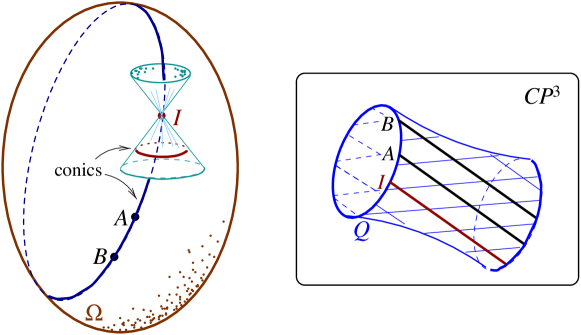
Figure 9: Time-like geodesics in Minkowski space. Each time-like geodesic in a flat four-dimensional space-time determines a quadric in projective twistor space. A quadric in ${\mathbb{P}}^{3}$ has two distinct systems of generators. In the case of a time-like geodesic, the line $I$ belongs to one of the two systems. The corresponding geodesic is a conic curve in the Klein quadric $\Omega$, and has the property that it passes through the point $I$. The second system of generators then corresponds to a polar conic that lies on the null cone infinity and does not go through $I$.

To pursue this point further, we recall that $\bar{\mathcal{H}}^{4}$ has the structure of a quadric $\Omega$ in ${\mathbb{P}}^{5}$. More specifically, for $r=2$ the space of skew rank two twistors is ${\mathbb{C}}^{6}$, which is projectively ${\mathbb{P}}^{5}$, and $\bar{\mathcal{H}}^{4}$ is the locus defined by the homogeneous quadratic equation

$$\varepsilon_{\alpha\beta\gamma\delta}X^{\alpha\beta}X^{\gamma\delta}=0.$$ (131)

Infinity in $\bar{\mathcal{H}}^{4}$ can then be defined by the intersection of $\bar{\mathcal{H}}^{4}$ in ${\mathbb{P}}^{5}$ with the projective 4-plane $I^{4}$ given by the equation

$$\varepsilon_{\alpha\beta\gamma\delta}I^{\alpha\beta}X^{\gamma\delta}=0.$$ (132)

If $I^{\alpha\beta}$ is simple, then $I^{4}$ is tangent to $\bar{\mathcal{H}}^{4}$, and the intersection is a cone—the null cone at infinity. The geometry of this space plays a crucial role in determining the properties of time-like geodesics in Minkowski space, as discussed in Figure 9.

On the other hand, if $I^{\alpha\beta}$ is not simple, then the intersection $I^{4}\cap\bar{\mathcal{H}}^{4}$ is a 3-quadric. The resulting geometry, if $I^{\alpha\beta}$ is real, is that of de Sitter space. The metric on $I^{4}\cap\bar{\mathcal{H}}^{4}$ in this case is given by

$${\rm d}s^{2}=\frac{\varepsilon_{\alpha\beta\gamma\delta}{\rm d}X^{\alpha\beta}{\rm d}X^{\gamma\delta}}{(\varepsilon_{\alpha\beta\gamma\delta}I^{\alpha\beta}X^{\gamma\delta})^{2}},$$ (133)

and the parameter $\lambda$ defined by (130) has the interpretation of being the associated cosmological constant. We note that ${\rm d}s$ is independent of the scale of $X^{\alpha\beta}$, and has an $I$-weight of $-1$, as is appropriate for an element of time. The de Sitter group consists of transformations of ${\mathbb{P}}^{5}$ that preserve both the quadric $\Omega$ and the point $I$.

With the incorporation of some additional structure at infinity, the entire class of Robertson-Walker cosmological models can be represented in a similar way Hurd1 ; Hurd2 ; Penrose1 ; Penrose6 ; Penrose8 ; Penrose9 . The idea can be described briefly as follows. We start with the complex projective space ${\mathbb{P}}^{5}$ and in it the quadric $\Omega$ defined by (131). The points of space-time are given by a reality structure by requiring that $\overline{X}^{\alpha\beta}=X^{\alpha\beta}$. Next we introduce a pencil of 4-planes in ${\mathbb{P}}^{5}$ of the form

$$Z_{\alpha\beta}=pP_{\alpha\beta}+qQ_{\alpha\beta},$$ (134)

where $(p,q)\in{\mathbb{C}}^{2}-\{0,0\}$. For each such $Z_{\alpha\beta}$, the intersection of the 4-plane

$$Z_{\alpha\beta}X^{\alpha\beta}=0$$ (135)

with the real quadric given by

$$\epsilon_{\alpha\beta\gamma\delta}X^{\alpha\beta}X^{\gamma\delta}=0\quad{\rm and}\quad\overline{X}^{\alpha\beta}=X^{\alpha\beta}$$ (136)

defines a certain subspace of the space-time. For certain choices of $\{P_{\alpha\beta},Q_{\alpha\beta},p,q\}$ the resulting subspace can be interpreted (in some cases with the deletion of certain elements) as a constant-time space-like hypersurface $\sigma^{3}$ in the space-time. The corresponding cosmological model is then obtained by selecting a one-parameter ‘chronological family’ of such surfaces, and choosing an appropriate conformal factor for the metric geometry.

In more detail, the construction is as follows. For $k=1$ (a closed universe) we require the skew twistors $P_{\alpha\beta}$ and $Q_{\alpha\beta}$ to be complex and to satisfy the following relations:

$$\epsilon^{\alpha\beta\gamma\delta}P_{\alpha\beta}P_{\gamma\delta}=0,\quad\epsilon^{\alpha\beta\gamma\delta}Q_{\alpha\beta}Q_{\gamma\delta}=0,\quad{\rm and}\quad P_{\alpha\beta}=\overline{Q}_{\alpha\beta}.$$ (137)

We then let $p={\rm e}^{{\rm i}\theta}$, $q={\rm e}^{-{\rm i}\theta}$ for some $\theta\in[0,2\pi]$. The resulting one-parameter family of surfaces determined by

$$Z_{\alpha\beta}={\rm e}^{{\rm i}\theta}P_{\alpha\beta}+{\rm e}^{-{\rm i}\theta}\overline{P}_{\alpha\beta}$$ (138)

has the property that each is a 3-sphere. For a $k=-1$ cosmology we require

$$\epsilon^{\alpha\beta\gamma\delta}P_{\alpha\beta}P_{\gamma\delta}=0,\quad\epsilon^{\alpha\beta\gamma\delta}Q_{\alpha\beta}Q_{\gamma\delta}=0,\quad P_{\alpha\beta}=\overline{P}_{\alpha\beta},\quad{\rm and}\quad Q_{\alpha\beta}=\overline{Q}_{\alpha\beta}.$$ (139)

In this case the relevant family of 4-planes is given by (134) with $(p,q)\in{\mathbb{R}}^{2}-\{0,0\}$, the overall scale of $Z_{\alpha\beta}$ being unimportant. For $k=0$ we set

$$\epsilon^{\alpha\beta\gamma\delta}P_{\alpha\beta}P_{\gamma\delta}=0,\quad\epsilon^{\alpha\beta\gamma\delta}Q_{\alpha\beta}Q_{\gamma\delta}=1,\quad P_{\alpha\beta}=\overline{P}_{\alpha\beta},\quad{\rm and}\quad Q_{\alpha\beta}=\overline{Q}_{\alpha\beta},$$ (140)

with $(p,q)$ as above in the $k=-1$ case.

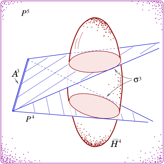
Figure 10: Friedmann-Robertson-Walker cosmologies. In the case $k=1$ depicted here the chronology of the FRW cosmology is generated by a pencil of projective 4-planes hinged on an axis ${\mathcal{A}}^{3}$ in ${\mathbb{P}}^{5}$. The axis is chosen so that it does not impinge on any of the real points of the space-time. As a consequence the constant-time hypersurfaces in the cosmological model are compact.

In each case we can consider the ‘axis’ obtained by intersecting the elements of the given family of 4-planes. In the $k=+1$ case, the axis itself does not intersect the associated real space-time, and as a consequence the resulting hypersurfaces of constant time are topologically 3-spheres (see Figure 10). In the $k=0$ case the axis ‘touches’ the space-time at a point (given by $q=0$) common to all of the intersection spaces. If we remove this point (or treat it as a point at infinity), then the resulting constant-time surfaces are each topologically ${\mathbb{R}}^{3}$. In the $k=-1$ case, the common intersection region is a 2-sphere, and as a consequence an ‘open’ cosmological model results in this case as well.

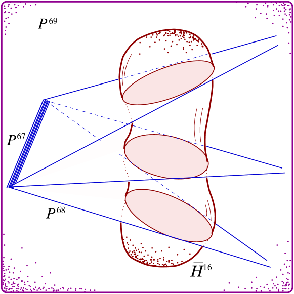
Figure 11: Chronological foliation of an $r=4$ hypercosmology. The compactified quantum space-time $\bar{\mathcal{H}}^{16}$ is a real submanifold of the complex projective space ${\mathbb{P}}^{69}$. A pencil of ${\mathbb{P}}^{68}$-hyperplanes hinged on a complex axis ${\mathbb{P}}^{67}$ intersects the space-time in a set of hypersurfaces. Depending on the reality structure of the pencil, and its real subparameterisation, a variety of different possibilities can emerge for the global structure of the hypersurface family.

Thus we see that the algebraic geometry of twistor theory gives us an essentially ‘unified’ point of view over the various standard cosmological models—this approach can be pursued at greater length, giving rise to a geometrical characterisation of the different types of situations that can occur, depending, in particular, on the global structure and topology of the space-time, on the equation of state of the fluid representation in the energy tensor, and on the type of cosmological constant (if any) in the model. Much more detail, along with specific examples for various choices of the equation of state, can be found in Hurd1 ; Hurd2 ; Penrose6 ; Penrose9 .

It is interesting to note that more or less the same state of affairs prevails in higher dimensions (see Figure 11 for an example of a sixteen-dimensional class of ‘quantum cosmologies’ analogous to the $k=1$ Friedmann-Robertson-Walker models). In other words, the choice of structure at infinity gives rise to various possible global structures for the quantum space-time, and in particular, to a chronometric form that is in general not flat, thus making $\bar{\mathcal{H}}^{r^{2}}$ a cosmological model. In the case of a standard four-dimensional cosmological model based on Einstein’s theory, the existence of structure at (or ‘beyond’) infinity has a bearing on the geometry of space-time alone. In the case of a quantum cosmology, however, the structure at infinity also has implications for microscopic physics. For instance, whereas in the four-dimensional de Sitter cosmology the relevant structure at infinity contains the ‘invariant’ information of one dimensional constant (the cosmological constant), in the higher-dimensional situation there are in general a number of such constants that may emerge as geometrical invariants of the theory. Thus within a single geometric framework one has the scope for introducing structure (or what amounts to the same thing—the breaking of symmetry) both on a global or cosmological scale, as well as on the microscopic scales of distance, time, and energy associated with the phenomenology of elementary particles. One might say that in these models the structure at infinity is playing the role of the Higgs fields. One can even envisage the possibility of explaining, in a purely geometrical language, the basis of the remarkable coincidences involving various fundamental constants of nature that have puzzled physicists for many decades.

13 Weak and strong Hermiticity

As a prelude to our discussion of the idea of symmetry breaking in quantum space-time, we digress briefly to review the notions of weak and strong Hermiticity. This material is relevant to the origin of unitarity in quantum mechanics. Intuitively speaking, we observe that when the weak Hermiticity condition is imposed on a hyperspinor $x^{\,AA^{\prime}}$ representing a space-time event, then $x^{\,AA^{\prime}}$ belongs to the real subspace ${\mathbb{R}}^{AA^{\prime}}$. As such, the hyper-relativistic symmetry of quantum space-time is not affected by the imposition of this condition. If, however, we break the hyper-relativistic symmetry by selecting a preferred time-like direction, then we can speak of a stronger reality condition whereby an isomorphism is established between the primed and unprimed hyperspin spaces.

We begin with the weak Hermitian property. Let ${\mathbb{S}}^{A}$ denote, as before, an $r$-dimensional complex vector space. We also introduce the associated spaces ${\mathbb{S}}_{A}$, ${\mathbb{S}}^{A^{\prime}}$, and ${\mathbb{S}}_{A^{\prime}}$. In general, there is no natural isomorphism between ${\mathbb{S}}^{A^{\prime}}$ and ${\mathbb{S}}_{A}$. Therefore, there is no natural matrix multiplication law or trace operation defined for elements of ${\mathbb{S}}^{A}\otimes{\mathbb{S}}^{A^{\prime}}$. Nevertheless, certain matrix operations are well defined. For example, the determinant of a generic element $\mu^{AA^{\prime}}$ is given by

$$\det(\mu)=\frac{1}{r!}\,\varepsilon_{AB\cdots C}\,\varepsilon_{A^{\prime}B^{\prime}\cdots C^{\prime}}\,\mu^{AA^{\prime}}\mu^{BB^{\prime}}\cdots\mu^{CC^{\prime}}.$$ (141)

The weak Hermitian property is also well-defined. In particular, if ${\bar{\mu}}^{A^{\prime}A}$ is the complex conjugate of $\mu^{AA^{\prime}}$, then we say that $\mu^{AA^{\prime}}$ is weakly Hermitian if $\mu^{AA^{\prime}}={\bar{\mu}}^{A^{\prime}A}$. As we have observed, for many applications, weak Hermiticity suffices.

Now we consider the strong Hermitian property. In some situations there may exist a natural map ${\mathbb{S}}^{A^{\prime}}\to{\mathbb{S}}_{A}$ defined by the context of the particular problem. Such a map is called a Hermitian correlation. In this case, the complex conjugate of an element $\alpha^{A}\in{\mathbb{S}}^{A}$ determines an element ${\bar{\alpha}}_{A}\in{\mathbb{S}}_{A}$. For any element $\mu^{A}_{B}\in{\mathbb{S}}^{A}\otimes{\mathbb{S}}_{B}$ we define the operations of determinant, matrix multiplication, and trace in the usual manner. The determinant is

$$\det(\mu)=\frac{1}{r!}\,\varepsilon_{AB\cdots C}\,\varepsilon^{PQ\cdots R}\,\mu^{A}_{P}\mu^{B}_{Q}\cdots\mu^{C}_{R},$$ (142)

and the Hermitian conjugate of $\mu^{A}_{\ B}$ is ${\bar{\mu}}_{A}^{\ B}$. The Hermitian correlation is given by the choice of a preferred element $t_{AA^{\prime}}\in{\mathbb{S}}_{A}\otimes{\mathbb{S}}_{A^{\prime}}$. Then we write

$${\bar{\alpha}}_{A}=t_{AA^{\prime}}{\bar{\alpha}}^{A^{\prime}},$$ (143)

where ${\bar{\alpha}}_{A}$ is now called the complex conjugate of $\alpha^{A}$. When there is a Hermitian correlation ${\mathbb{S}}^{A^{\prime}}\leftrightarrow{\mathbb{S}}_{A}$, we call the condition $\mu^{A}_{\ B}={\bar{\mu}}^{A}_{\ B}$ the strong Hermitian property.

Thus once we break the relativistic invariance by introducing a preferred element $t_{AA^{\prime}}$ that determines a Hermitian correlation, we may carry out specific calculations in that frame. To gain a better understanding of this, consider an event in complex Minkowski space defined by its separation $x^{{\bf AA}^{\prime}}$ from the origin. The complex conjugate of $x^{{\bf AA}^{\prime}}$ is ${\bar{x}}^{{\bf AA}^{\prime}}$, so $x^{{\bf AA}^{\prime}}$ is real if $x^{{\bf AA}^{\prime}}={\bar{x}}^{{\bf AA}^{\prime}}$. Let $t^{{\bf AA}^{\prime}}$ be a fixed time-like vector satisfying $g_{\rm ab}t^{\rm a}t^{\rm b}=2$. With respect to this choice of $t^{{\bf AA}^{\prime}}$, the trace of $x^{{\bf AA}^{\prime}}$ is defined by

$${\rm tr}(x^{{\bf AA}^{\prime}})=x^{{\bf AA}^{\prime}}t_{{\bf AA}^{\prime}}.$$ (144)

Once $t^{{\bf AA}^{\prime}}$ is fixed, we may represent $x^{{\bf AA}^{\prime}}$ in terms of Pauli matrices, according to which $x^{{\bf AA}^{\prime}}$ admits a matrix representation of the form (4). The time variable is then given by $t=\frac{1}{2}{\rm tr}(x^{{\bf AA}^{\prime}})$ and the Minkowski metric is given by the determinant (5). We can also define a commutator for a pair of space-time position vectors $x^{{\bf AA}^{\prime}}$ and $y^{{\bf AA}^{\prime}}$ by setting

$$z^{{\bf AA}^{\prime}}=\left(x^{{\bf AB}^{\prime}}y^{{\bf BA}^{\prime}}-y^{{\bf AB}^{\prime}}x^{{\bf BA}^{\prime}}\right)t_{{\bf BB}^{\prime}}.$$ (145)

The geometrical meaning of (145) is that $z^{{\bf AA}^{\prime}}$ corresponds to the ordinary 3-space cross-product of the projection of the vectors $x^{{\bf AA}^{\prime}}$ and $y^{{\bf AA}^{\prime}}$ onto the space-like hyperplane orthogonal to $t^{{\bf AA}^{\prime}}$ that passes through the origin. Analogously, we can discuss the ‘spectral’ properties of vectors with respect to a given choice of $t^{{\bf AA}^{\prime}}$ and a given choice of origin in space-time. The two eigenvalues of $x^{{\bf AA}^{\prime}}$ are then given by $t\pm\sqrt{x^{2}+y^{2}+z^{2}}$. Thus two such vectors $x^{{\bf AA}^{\prime}}$ and $y^{{\bf AA}^{\prime}}$ are isospectral if and only if they lie on a common sphere about the origin lying in the given space-like hyperplane. Similar remarks apply to higher-dimensional quantum space-times.

14 Symmetry breaking mechanism

Now we proceed to introduce a natural mechanism for symmetry breaking that arises in the case of a standard ‘flat’ quantum space-time endowed with the canonical structures associated with reality and infinity. We shall make the point in particular that the breaking of symmetry in quantum space-time is intimately linked to the notion of quantum entanglement. According to this point of view the introduction of symmetry-breaking in the early stages of the universe can be understood as a phase transition, or a sequence of phase transitions, the ultimate consequence of which is an approximate disentanglement of a four-dimensional ‘classical’ space-time.

In practical terms the breaking of symmetry is represented in our framework by an ‘index decomposition’. In particular, if the dimension $r$ of the hyperspin space is not a prime number, then a natural method of breaking the symmetry arises by consideration of the decomposition of $r$ into factors. The specific essential assumption that we shall make at this juncture will be that the dimension of the hyperspin space ${\mathbb{S}}^{A}$ is even. Then we write $r=2n$, where $n=1,2,\ldots$, and set

$${\mathbb{S}}^{A}={\mathbb{S}}^{{\bf A}i},$$ (146)

where ${\bf A}$ is a standard two-component spinor index, and $i$ will be called an ‘internal’ index $(i=1,2,\ldots,n)$. Thus we can write ${\mathbb{S}}^{{\bf A}i}={\mathbb{S}}^{{\bf A}}\otimes{\mathbb{H}}^{i}$, where ${\mathbb{S}}^{{\bf A}}$ is a standard spin space of dimension two, and ${\mathbb{H}}^{i}$ is a complex vector space of dimension $n$. The breaking of the symmetry then amounts to the fact that we can identify the hyperspin space with the tensor product of these two spaces.

We shall assume, moreover, that ${\mathbb{H}}^{i}$ is endowed with a strong Hermitian structure, i.e. we shall assume that there is a canonical anti-linear isomorphism between the complex conjugate of the internal space ${\mathbb{H}}^{i}$ and the dual space ${\mathbb{H}}_{i}$. If $\psi^{i}\in{\mathbb{H}}^{i}$, then we write ${\bar{\psi}}_{i}$ for the complex conjugate of $\psi^{i}$, where ${\bar{\psi}}_{i}\in{\mathbb{H}}_{i}$. We see therefore that ${\mathbb{H}}^{i}$ is a complex Hilbert space—and indeed although here we consider for technical simplicity the case for which $n$ is finite, one should have in mind also the general infinite dimensional situation. For the other hyperspin spaces we write

$${\mathbb{S}}_{A}={\mathbb{S}}_{{\bf A}i},\quad{\mathbb{S}}^{A^{\prime}}={\mathbb{S}}^{{\bf A}^{\prime}}_{\ \ i},\quad{\rm and}\quad{\mathbb{S}}_{A^{\prime}}={\mathbb{S}}_{{\bf A}^{\prime}}^{\ \ i},$$ (147)

respectively. These equivalences preserve the duality between ${\mathbb{S}}^{A}$ and ${\mathbb{S}}_{A}$, and between ${\mathbb{S}}^{A^{\prime}}$ and ${\mathbb{S}}_{A^{\prime}}$; and at the same time are consistent with the complex conjugation relations between ${\mathbb{S}}^{A}$ and ${\mathbb{S}}^{A^{\prime}}$, and between ${\mathbb{S}}_{A}$ and ${\mathbb{S}}_{A^{\prime}}$. Hence if $\alpha^{{\bf A}i}\in{\mathbb{S}}^{{\bf A}i}$ then under complex conjugation we have $\alpha^{{\bf A}i}\to{\bar{\alpha}}^{{\bf A}^{\prime}}_{\ \ i}$, and if $\beta_{{\bf A}i}\in{\mathbb{S}}_{{\bf A}i}$ then $\beta_{{\bf A}i}\to{\bar{\beta}}_{{\bf A}^{\prime}}^{\ \ i}$.

In the case of a quantum space-time vector $r^{\,AA^{\prime}}$ we have a corresponding structure induced by the identification

$$r^{\,AA^{\prime}}=r^{{\bf AA}^{\prime}i}_{\ \ \ \ \ j}.$$ (148)

When the quantum space-time vector is real, the weak Hermitian structure on $r^{\,AA^{\prime}}$ is manifested in the form of a standard weak Hermitian structure on the two-component spinor index pair, together with a strong Hermitian structure on the internal index pair. In other words, the Hermitian condition on the space-time vector $r^{\,AA^{\prime}}$ is given by

$${\bar{r}}^{{\bf A}^{\prime}{\bf A}\ \ i}_{\ \ \ \ \ j}=r^{{\bf AA}^{\prime}i}_{\ \ \ \ \ j}.$$ (149)

One consequence of these relations is that we can interpret each point in quantum space-time as being a space-time valued operator. The ordinary classical space-time then ‘sits’ inside the quantum space-time in a canonical manner—namely, as the locus of those points of quantum space-time that factorise into the product of a space-time point $x^{{\bf AA}^{\prime}}$ and the identity operator on the internal space:

$$x^{{\bf AA}^{\prime}i}_{\ \ \ \ \ j}=x^{{\bf AA}^{\prime}}\delta^{i}_{\ j}.$$ (150)

Thus, in situations where special relativity is a satisfactory theory, we regard the relevant events as taking place on or in the immediate neighbourhood of this embedding of Minkowski space in ${\mathcal{H}}^{4n^{2}}$.

This picture can be presented in more geometric terms as follows. The hypertwistor space ${\mathbb{P}}^{2r-1}$ in the case $r=2n$ admits a Segré embedding of the form

$${\mathbb{P}}^{3}\times{\mathbb{P}}^{n-1}\subset{\mathbb{P}}^{4n-1}.$$ (151)

Many such embeddings are possible, though they are all equivalent to one another under the action of the overall symmetry group $U(2n,2n)$. If the symmetry is broken and one such embedding is selected out, then following the conventions discussed earlier we can introduce homogeneous coordinates and write $Z^{\alpha i}$ for the hypertwistor. Here the Greek letter ${\alpha}$ denotes an ordinary twistor index $({\alpha}=0,1,2,3)$ and $i$ denotes an internal index $(i=1,2,\ldots,n)$. These two indices, when clumped together, constitutes a hypertwister index. The Segré embedding consists of those points in ${\mathbb{P}}^{4n-1}$ for which we have a product decomposition of the associated hypertwistor given by

$$Z^{\alpha i}=Z^{\alpha}\psi^{i}.$$ (152)

The idea of symmetry breaking that we are putting forward here is related to the notion of disentanglement in standard quantum mechanics (cf. Gibbons 1992; Brody & Hughston 2001). That is to say, at the unified level the degrees of freedom associated with space-time symmetry are quantum mechanically entangled with the internal degrees of freedom associated with microscopic physics. The phenomena responsible for the breakdown of symmetry are thus analogous to the mechanisms of decoherence through which quantum entanglements are gradually diminished. Some readers may raise the objection that surely it is impossible to unify the unitary symmetries of elementary particle phenomenology with the symmetries of space-time (cf., e.g., Coleman ). It should be noted, however, that our approach is not to attempt to embed a relativistic symmetry group in a higher-dimensional unitary group, but rather to embed the unitary group in a higher-dimensional relativistic symmetry group. Our methodology is consistent with the point of view put forward by Penrose that for a coherent unification of general relativity and quantum mechanics, the rules of quantum theory must undergo ‘profound modification’ Penrose7 .

The compactified complexified quantum space-time ${\mathcal{C}}\!\bar{\mathcal{H}}^{4n^{2}}$ can be regarded as the aggregate of projective $(2n-1)$-planes in ${\mathbb{P}}^{4n-1}$. Now generically a ${\mathbb{P}}^{2n-1}$ in ${\mathbb{P}}^{4n-1}$ will not intersect the Segré variety

$${\mathcal{G}}^{n+2}={\mathbb{P}}^{3}\times{\mathbb{P}}^{n-1}.$$ (153)

Such a generic $(2n-1)$-plane corresponds to a generic point in ${\mathcal{C}}\!\bar{\mathcal{H}}^{4n^{2}}$. The $(2n-1)$-planes that correspond to the points of compactified complexified Minkowski space can be constructed as follows. For each line $L$ in ${\mathbb{P}}^{3}$ we consider the subvariety ${\mathcal{G}}_{L}^{n}\subset{\mathcal{G}}^{n+2}$ where ${\mathcal{G}}_{L}^{n}={\mathbb{P}}_{L}^{1}\times{\mathbb{P}}^{n-1}$. For any algebraic variety $V^{j}\subset{\mathbb{P}}^{l}$ $(j\leq l-1)$ we define the span of $V^{j}$ to be the projective plane spanned by the points of $V^{j}$. We say a point $X$ in the ambient space ${\mathbb{P}}^{l}$ lies in the span of the variety $V^{j}$ if and only if there exist $m$ points in $V^{j}$ for some $m\geq 2$ with the property that $X$ lies in the $(m-1)$-plane spanned by those $m$ points. The dimension $k$ of the span of $V^{j}$ satisfies $j\leq k\leq l$; however, the value of $k$ depends on the geometry of $V^{j}$.

The linear span of the points in ${\mathcal{G}}_{L}^{n}$, for any given $L$, is a $(2n-1)$-plane. This is the ${\mathbb{P}}_{L}^{2n-1}$ in ${\mathbb{P}}^{4n-1}$ that represents the point in $\bar{\mathcal{H}}^{4n^{2}}$ corresponding to the line $L$ in ${\mathbb{P}}^{3}$. The aggregate of such special $(2n-1)$-planes, defined by their intersection properties with the Segré variety ${\mathcal{G}}^{n+2}$, constitutes a submanifold of ${\mathcal{C}}\!\bar{\mathcal{H}}^{4n^{2}}$, and this submanifold is compactified complexified Minkowski space ${\mathcal{C}}\!\bar{\mathcal{H}}^{4}$. Thus we see that once the symmetry of quantum space-time ${\mathcal{C}}\!{\mathcal{H}}^{4n^{2}}$ has been broken in the particular way we have discussed, then ordinary Minkowski space can be identified as a submanifold.

Let us now consider the implications of our symmetry breaking mechanism for fields defined on quantum space-time. As an example, let $\phi(x^{\,AA^{\prime}})$ be a scalar field on quantum space-time. After we break the symmetry by writing $x^{\,AA^{\prime}}=x^{{\bf AA}^{\prime}i}_{\ \ \ \ \ j}$, we consider a Taylor expansion of the field around the embedded Minkowski space-time. Specifically, for such an expansion we have

$$\phi(x^{\,AA^{\prime}})=\phi^{(0)}(x^{{\bf AA}^{\prime}})+\phi^{(1)\ i}_{{\bf AA}^{\prime}\ j}(x^{\,{\bf AA}^{\prime}})\left(x^{{\bf AA}^{\prime}j}_{\ \ \ \ \ i}-x^{{\bf AA}^{\prime}}\delta^{j}_{\ i}\right)+\cdots,$$ (154)

where

$$\phi^{(0)}(x^{{\bf AA}^{\prime}})=\phi(x^{\,AA^{\prime}})\Big{|}_{x^{\,AA^{\prime}}=x^{{\bf AA}^{\prime}}\delta^{j}_{\ i}}\ ,$$ (155)

and

$$\phi^{(1)\ i}_{{\bf AA}^{\prime}\ j}(x^{\,{\bf AA}^{\prime}})=\left.\frac{\partial\phi}{\partial x^{{\bf AA}^{\prime}j}_{\ \ \ \ \ i}}\right|_{x^{{\bf AA}^{\prime}j}_{\ \ \ \ \ i}=x^{{\bf AA}^{\prime}}\delta^{j}_{\ i}}.$$ (156)

Therefore, the order zero term has the character of a classical field on Minkowski space, and the first order term can be interpreted as a ‘multiplet’ of fields, transforming according to the adjoint representation of the internal symmetry group $U(n)$.

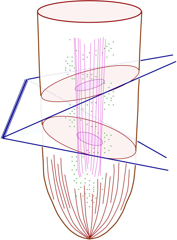
Figure 12: Symmetry breaking and matter formation in a hypertwistorial quantum cosmology. In its earliest stages the universe is highly symmetrical. Eventually, symmetry is broken, and a four-dimensional ‘classical’ cosmology freezes out, becoming largely disentangled from the reminder of the quantum space-time. The formation of matter during the disentanglement process may not be confined to the four-dimensional subspace. If such a scenario prevails, the bulk of this ‘dark material’ is likely to remain outside the four-dimensional subspace, though nevertheless having an impact on its dynamics.

In this connection we note that the symmetry breaking mechanism that we have proposed here has yet another representation—namely, the expression of a hypertwistor as a multi-twistor system, i.e. as a multiplet of Penrose twistors. The physical and geometrical characteristics of such $n$-twistor systems have been analysed at great length by a number of authors (see, e.g., Hughston2 ; Hughston3 ; Penrose3 ; Penrose4 ; Penrose5 ; Sparling ; Tod1 and references cited therein), and it is interesting therefore to see the direct link with hypertwistor theory and quantum space-time geometry. It is fitting also to make a tribute here to the work of Zoltan Perjés, whose extensive contributions to relativity theory include, in particular, a number of important studies concerning the properties of $n$-twistor systems and their symmetries Lukacs ; Perjes1 ; Perjes2 ; Perjes3 ; Perjes4 ; Perjes5 ; Perjes6 ; Perjes7 ; Perjes8 ; Perjes9 ; Perjes10 ; Perjes11 ; Tod2 .

It is tempting to speculate that even in a more dynamic context some version of the symmetry breaking mechanism provided here will manifest itself. In this picture we would envisage the earliest stages of the universe as being highly symmetrical, rather in the spirit of Penrose’s Weyl curvature hypothesis Penrose11 ; Penrose12 , with no appreciable distinction between the conventional space-time degrees of freedom and the internal degrees of freedom associated with quantum theory. Nevertheless, the causal geometry of the universe remains well defined, and it is interesting to ask whether there might be some scenario within the rather rich causal structure of a quantum space-time that would allow us to account for the so-called ‘horizon problem’. In any event, once symmetry breaking takes place—and this may happen in stages, corresponding to a successive factorisation of the underlying hypertwistor space—then it makes sense to think of ordinary four-dimensional space-time as becoming more or less disentangled from the rest of the universe, and behaving in a way that is to some extent autonomous. Nonetheless, we might reasonably expect its global dynamics, on a cosmological scale, to be affected by the distribution of mass and energy elsewhere in the quantum space-time as well (see, e.g., Figure 12).

15 Emergence of quantum probability

The embedding of Minkowski space in the quantum space-time ${\mathcal{H}}^{4n^{2}}$ given by (150) implies a corresponding embedding of the Poincaré group in the hyper-Poincaré group. This can be seen as follows. The standard Poincaré group in ${\mathcal{H}}^{4}$ consists of transformations of the form

$$x^{{\bf AA}^{\prime}}\longrightarrow\,\lambda^{\bf A}_{\bf B}\,\bar{\lambda}^{{\bf A}^{\prime}}_{{\bf B}^{\prime}}\,x^{{\bf BB}^{\prime}}+\beta^{{\bf AA}^{\prime}},$$ (157)

and the hyper-Poincaré transformations in ${\mathcal{H}}^{4n^{2}}$ are of the form

$$x^{{\bf AA}^{\prime}i}_{\ \ \ \ \ j}\longrightarrow\,\lambda^{\bf A}_{\bf B}\,\bar{\lambda}^{{\bf A}^{\prime}}_{{\bf B}^{\prime}}\,x^{{\bf BB}^{\prime}i}_{\ \ \ \ \ j}+\beta^{{\bf AA}^{\prime}}\delta^{i}_{\,j}.$$ (158)

With the identification $A={\bf A}i$, the general hyper-Poincaré transformation in the broken symmetry phase can be expressed in the form

$$x^{{\bf AA}^{\prime}i}_{\ \ \ \ \ j}\longrightarrow\,L^{{\bf A}i}_{{\bf B}k}\,\bar{L}^{{\bf A}^{\prime}l}_{{\bf B}^{\prime}j}\,x^{{\bf BB}^{\prime}k}_{\ \ \ \ \ l}+\beta^{{\bf AA}^{\prime}i}_{\ \ \ \ \ j}.$$ (159)

Thus the embedding of the Poincaré group as a subgroup of the hyper-Poincaré group is given by

$$L^{{\bf A}i}_{{\bf B}j}=\lambda^{\bf A}_{\bf B}\delta^{i}_{\ j}\quad{\rm and}\quad\beta^{{\bf AA}^{\prime}i}_{\ \ \ \ \ j}=\beta^{{\bf AA}^{\prime}}\delta^{i}_{\,j}.$$ (160)

Bearing this in mind, we now construct a class of maps from the general even-dimensional quantum space-time ${\mathcal{H}}^{4n^{2}}$ to Minkowski space ${\mathcal{H}}^{4}$. It turns out Brody2 that under rather general physical assumptions such maps are necessarily of the form

$$x^{{\bf AA}^{\prime}i}_{\ \ \ \ \ j}\longrightarrow\,x^{{\bf AA}^{\prime}}=\rho^{j}_{i}\,x^{{\bf AA}^{\prime}i}_{\ \ \ \ \ j},$$ (161)

where $\rho^{j}_{i}$ is a density matrix. As usual, by a density matrix we mean a positive semi-definite Hermitian matrix with unit trace. Thus the maps arising here can be regarded as quantum expectations.

In particular, let $\rho:\ {\mathcal{H}}^{4n^{2}}\to{\mathcal{H}}^{4}$ satisfy the following conditions: (i) $\rho$ is linear and maps the origin of ${\mathcal{H}}^{4n^{2}}$ to the origin of ${\mathcal{H}}^{4}$; (ii) $\rho$ is Poincaré invariant; and (iii) $\rho$ preserves causal relations. Then $\rho$ is given by a density matrix on the internal space.

The general linear map from ${\mathcal{H}}^{4n^{2}}$ to ${\mathcal{H}}^{4}$ preserving the origin is given by

$$x^{{\bf AA}^{\prime}i}_{\ \ \ \ \ j}\longrightarrow\,x^{{\bf AA}^{\prime}}=\rho^{{\bf AA}^{\prime}j}_{{\bf BB}^{\prime}i}\,x^{{\bf BB}^{\prime}i}_{\ \ \ \ \ j},$$ (162)

where $\rho^{{\bf AA}^{\prime}j}_{{\bf BB}^{\prime}i}$ is weakly Hermitian. Now suppose that we subject ${\mathcal{H}}^{4n^{2}}$ to a Poincaré transformation of the form (158), and require the corresponding transformation of ${\mathcal{H}}^{4}$ should be of the form (157). If $\rho$ satisfies these conditions then we shall say that the map $\rho$ is Poincaré invariant. Clearly, Poincaré invariance holds if and only if

$$\rho^{{\bf AA}^{\prime}j}_{{\bf BB}^{\prime}i}\left(\lambda^{\bf B}_{\bf C}\,\bar{\lambda}^{{\bf B}^{\prime}}_{{\bf C}^{\prime}}\,x^{{\bf CC}^{\prime}i}_{\ \ \ \ \ j}+b^{{\bf BB}^{\prime}}\delta^{i}_{\,j}\right)=\lambda^{\bf A}_{\bf B}\,\bar{\lambda}^{{\bf A}^{\prime}}_{{\bf B}^{\prime}}\left(\rho^{{\bf BB}^{\prime}j}_{{\bf CC}^{\prime}i}\,x^{{\bf CC}^{\prime}i}_{\ \ \ \ \ j}\right)+\beta^{{\bf AA}^{\prime}}$$ (163)

for all $\lambda^{\bf A}_{\bf B}\in SL(2n,{\mathbb{C}})$, for all $\beta^{{\bf AA}^{\prime}}\in{\mathbb{S}}^{{\bf AA}^{\prime}}$, and for all $x^{{\bf AA}^{\prime}i}_{\ \ \ \ \ j}\in{\mathcal{H}}^{4n^{2}}$. Thus we have

$$\rho^{{\bf AA}^{\prime}j}_{{\bf BB}^{\prime}i}\,\lambda^{\bf B}_{\bf C}\,\bar{\lambda}^{{\bf B}^{\prime}}_{{\bf C}^{\prime}}=\lambda^{\bf A}_{\bf B}\,\bar{\lambda}^{{\bf A}^{\prime}}_{{\bf B}^{\prime}}\,\rho^{{\bf BB}^{\prime}j}_{{\bf CC}^{\prime}i}$$ (164)

for all $\lambda^{\bf A}_{\bf B}$, and

$$\rho^{{\bf AA}^{\prime}j}_{{\bf BB}^{\prime}i}\,\delta^{i}_{\,j}\,\beta^{{\bf BB}^{\prime}}=\beta^{{\bf AA}^{\prime}}$$ (165)

for all $\beta^{{\bf AA}^{\prime}}$. Equation (164) implies that $\rho$ is of the form

$$\rho^{{\bf AA}^{\prime}j}_{{\bf BB}^{\prime}i}=\delta^{\bf A}_{\,\bf B}\,\delta^{{\bf A}^{\prime}}_{\,{\bf B}^{\prime}}\,\rho^{j}_{i}$$ (166)

for some $\rho^{j}_{i}$. Then (165) implies that $\rho$ must satisfy the trace condition $\rho^{i}_{i}=1$. Finally we require that if $x^{{\bf AA}^{\prime}i}_{\ \ \ \ \ j}$ and $y^{{\bf AA}^{\prime}i}_{\ \ \ \ \ j}$ are quantum space-time points with the property that the interval

$$r^{{\bf AA}^{\prime}i}_{\ \ \ \ \ j}=x^{{\bf AA}^{\prime}i}_{\ \ \ \ \ j}-y^{{\bf AA}^{\prime}i}_{\ \ \ \ \ j}$$ (167)

is future-pointing then $r^{{\bf AA}^{\prime}}=x^{{\bf AA}^{\prime}}-y^{{\bf AA}^{\prime}}$ is also future pointing, where

$$r^{{\bf AA}^{\prime}}=\rho^{j}_{i}\,r^{{\bf AA}^{\prime}i}_{\ \ \ \ \ j}.$$ (168)

This is the requirement that $\rho$ should be a ‘causal’ map. This condition implies that $\rho$ must be positive semi-definite. In particular, if $r^{{\bf AA}^{\prime}i}_{\ \ \ \ \ j}$ is future-pointing then it must be of the form

$$r^{{\bf AA}^{\prime}i}_{\ \ \ \ \ j}=\xi^{{\bf A}i}\bar{\xi}^{{\bf A}^{\prime}}_{j}+\eta^{{\bf A}i}\bar{\eta}^{{\bf A}^{\prime}}_{j}+\cdots.$$ (169)

Consider therefore the case for which $r^{{\bf AA}^{\prime}i}_{\ \ \ \ \ j}$ is null. Then we require that the expression $\xi^{{\bf A}i}\bar{\xi}^{{\bf A}^{\prime}}_{j}\rho^{j}_{i}$ should be future-pointing (or vanish) for any choice of $\xi^{{\bf A}i}$. In particular, we require that the vector $\xi^{{\bf A}i}\bar{\alpha}^{{\bf A}^{\prime}}_{j}\rho^{j}_{i}$ should be future-pointing if $\xi^{{\bf A}i}$ is of the form

$$\xi^{{\bf A}i}=\alpha^{\bf A}\psi^{i}$$ (170)

for any choice of $\xi^{\bf A}$ and $\psi^{i}$. This means that the inequality

$$\rho^{j}_{i}\psi^{i}\bar{\psi}_{j}\geq 0$$ (171)

holds for all $\psi^{i}$, which shows that $\rho^{j}_{i}$ is positive semi-definite. Since we have shown that the trace of $\rho^{j}_{i}$ is unity, it follows that $\rho^{j}_{i}$ is a density matrix.

This result shows how the causal structure of quantum space-time is linked with the probabilistic structure of quantum mechanics. The concept of a quantum state emerges when we ask for consistent ways of ‘averaging’ over the geometry of quantum space-time in order to obtain a reduced description of physical phenomena in terms of the geometry of Minkowski space. We see that a probabilistic interpretation of the map from a general quantum space-time to Minkowski space arises as a consequence of elementary causality requirements. We can thus view the space-time events in ${\mathcal{H}}^{4n^{2}}$ as representing quantum observables, the expectations of which correspond to points of ${\mathcal{H}}^{4}$.

References

- (1) Anandan, J. Aharonov, Y. 1990 Geometry of quantum evolution, Phys. Rev. Lett. 65, 1697-1700.
- (2) Ashtekar, A. Schilling, T. A. 1999 Geometrical formulation of quantum mechanics, in On Einstein’s Path (A. Harvey, ed.) Berlin: Springer-Verlag.
- (3) Borowiec, A. 1989 Comment on geometry of hyperspin manifolds, Int. J. Theor. Phys. 28, 1229-1232.
- (4) Borowiec, A. 1993 G-structure for hypermanifold, in Spinors, twistors, Clifford algebras and quantum deformations (Sobótka Castle, 1992, Z. Oziewicz, B. Jancewicz, & A. Borowiec, eds.) Fund. Theories Phys. 52, 75-79, Dordrecht: Kluwer.
- (5) Brody, D. C. & Hughston, L. P. 2001 Geometric quantum mechanics, J. Geom. Phys. 38, 19-53.
- (6) Brody, D. C. & Hughston, L. P. 2005 Theory of quantum space-time, Proc. R. Soc. London A461, (to appear).
- (7) Budinich, P. & Trautman, A. 1988 The spinorial chessboard, Berlin: Springer.
- (8) Cartan, É. 1937 Leçons sur la théorie des Spineurs Paris: Hermann & Cie. (English translation: The theory of spinors, Paris: Hermann & Cie., 1966 and New York: Dover, 1981).
- (9) Chevalley, C. 1954 The algebraic theory of spinors, New York: Columbia University Press.
- (10) Coleman, S. 1965 Trouble with relativistic , Phys. Rev. 138, B1262-B1267.
- (11) Eastwood, M. G., Penrose, R. & Wells, R. O. 1981 Cohomology and massless fileds, Commun. Math. Phys. 78, 305-351.
- (12) Ellis, J. 2003 Dark matter and dark energy: summary and future directions, Phil. Trans. R. Soc. London A361, 2607-2627.
- (13) Finkelstein, D. 1986 Hyperspin and hyperspace, Phys. Rev. Lett. 56, 1532-1533.
- (14) Finkelstein, D., Finkelstein, S. R. & Holm, C. 1986 Hyperspin manifolds, Int. J. Theor. Phys. 25, 441-463.
- (15) Finkelstein, D., Finkelstein, S. R. & Holm, C. 1987 Hypergravitational field equations, Phys. Rev. Lett. 59, 1265-1266.
- (16) Finkelstein, S. R. 1988 Gravity in hyperspin manifolds, Int. J. Theor. Phys. 27, 251-272.
- (17) Gibbons, G. W. 1992 Typical states and density matrices, J. Geom. Phys. 8, 147-162.
- (18) Holm, C. 1986 Christoffel formula and geodesic motion in hyperspin manifolds, Int. J. Theor. Phys. 25, 1209-1213.
- (19) Holm, C. 1988 The hyperspin structure of unitary groups, J. Math. Phys. 29, 978-986, Erratum 1989 ibid. 30, 2451.
- (20) Holm, C. 1988 Neutrino spectrum of Einstein universes, J. Math. Phys. 29, 2273-2279.
- (21) Holm, C. 1990 Connections in Bergmann manifolds, Int. J. Theor. Phys. 29, 23-36.
- (22) Hughston, L.P. 1979 Some new contour integral formulae, in Complex Manifold Techniques in Theoretical Physics (D. Lerner P. D. Sommers, eds.) San Francisco: Pitman.
- (23) Hughston, L.P. 1979 A derivation of the twistor internal symmetry group, in Advances in twistor theory (L. P. Hughston & R. S. Ward, eds.) San Francisco: Pitman.
- (24) Hughston, L.P. 1979 Twistors and Particles, Heidelberg: Springer.
- (25) Hughston, L.P. 1987 Applocations of SO(8) spinors, in Gravitation and Geometry (W. Rindler and A. Trautman, eds.) Naples: Bibliopolis.
- (26) Hughston, L.P. 1990 A remarkable connection between the wave equation and pure spinors in higher dimensions, in Further advances in twistor theory, vol. I: The Penrose transform and its applications (L. J. Mason & L. P. Hughston, eds.) Harlow: Longman.
- (27) Hughston, L.P. & Hurd, T. R. 1982 A calculus for space-time fields, Phys. Rep. 100, 273-326.
- (28) Hughston, L.P. & Mason, L. J. 1988 A generalised Kerr-Robinson theorem, Class. Quantum Grav. 5, 275-285.
- (29) Hughston, L. P., Penrose, R., Sommers, P. & Walker, M. 1971 On a quadratic first integral for the charged particle orbits in the charged Kerr solution, Commun. Math. Phys. 27, 303-308.
- (30) Hughston, L. P. & Sommers, P. 1973a Spacetimes with Killing tensors, Commun. Math. Phys. 32, 147-152.
- (31) Hughston, L. P. & Sommers, P. 1973b The Symmetries of Kerr black holes, Commun. Math. Phys. 33, 129-133.
- (32) Hurd, T. R. 1985 The projective geometry of simple cosmological models, Proc. R. Soc. London A397, 233-243.
- (33) Hurd, T. R. 1995 Cosmological models in , in Further advances in twistor theory, vol. II: Integrable systems, conformal geometry and gravitation (L. J. Mason, L. P. Hughston & P. Z. Kobak, eds.) Harlow: Longman.
- (34) Kibble, T. W. B. 1979 Geometrisation of quantum mechanics, Commun. Math. Phys. 65, 189-201.
- (35) Lukács, B., Perjés, Z., Sebestyén, A., Newman, E. T. & Porter, J. 1982 Structure of three-twistor particles, J. Math. Phys. 23, 2108-21?15.
- (36) Penrose, R. 1967 Twistor algebra, J. Math. Phys. 8, 345-366.
- (37) Penrose, R. 1968 Structure of space-time, in Battelle Rencontres (C. M. DeWitt and J. A. Wheeler, eds.) New York: W. A. Benjamin.
- (38) Penrose, R. 1975 Twistors and particles, in Quantum theory and the structure of time and space (L. Castell, M. Drieschner, & C. F. von Weizsacker, eds.) München: Carl Hanser Verlag.
- (39) Penrose, R. 1977 The twistor programme, Rep. Math. Phys. 12, 65-76.
- (40) Penrose, R. 1979 Singularities and time-asymmetry, in General relativity: an Einstein centenary survey (S. W. Hawking & W. Israel, eds.) Cambridge: Cambridge University Press.
- (41) Penrose, R. 1981 Time-asymmetry and quantum gravity, in Quantum Gravity 2 (C. J. Isham, R. Penrose, & D. W. Sciama, eds.) Oxford: Oxford University Press.
- (42) Penrose, R. 1995 Twistors for cosmological models, in Further advances in twistor theory, vol. II: Integrable systems, conformal geometry and gravitation (L. J. Mason, L. P. Hughston & P. Z. Kobak, eds.) Harlow: Longman.
- (43) Penrose, R. 1999 The central programme of twistor theory, Chaos, Solitons & Fractals 10, 581-611.
- (44) Penrose, R. & MacCallum, M. A. H. 1973 Twistor theory: an approach to the quantisation of fields and space-time, Phys. Rep. 6C, 241-315.
- (45) Penrose, R. & Rindler, W. 1984 Spinors and Space-time vol. 1, Cambridge: Cambridge University Press.
- (46) Penrose, R. & Rindler, W. 1986 Spinors and Space-time vol. 2, Cambridge: Cambridge University Press.
- (47) Penrose, R. & Sparling, G. A. J. 1979 A note on the -twistor internal symmetry group, in Advances in twistor theory (L. P. Hughston & R. S. Ward, eds.) San Francisco: Pitman.
- (48) Perjés, Z. 1975 Twistor variables of relativistic mechanics, Phys. Rev. D11, 2031-2041.
- (49) Perjés, Z. 1977 Perspectives of Penrose theory in particle physics, Rep. Math. Phys. 12, 193-211.
- (50) Perjés, Z. & Sparling, G. A. J. 1979 The twistor structure of hadrons, in Advances in twistor theory (L. P. Hughston & R. S. Ward, eds.) San Francisco: Pitman.
- (51) Perjés, Z. 1979 Unitary space of particle internal states, Phys. Rev. D20, 1857-1876.
- (52) Perjés, Z. 1981 Twistors and unitary space, in 85th Summer Meeting of AMS, American Mathematical Society, 457.
- (53) Perjés, Z. 1982 Twistor theory—a particle physicist attitude, Proc. 2nd Marcel Grossmann Conference (R. Ruffini, ed.) Amsterdam: North-Holland.
- (54) Perjés, Z. 1982 Internal symmetries in twistor theory, Czech. J. Phys. B32, 540-548.
- (55) Perjés, Z. & Sparling, G. A. J. 1982 An ISU(3) hadron mass formula, Surveys High Energ. Phys. 3, 27-37.
- (56) Perjés, Z. 1983 Twistor internal symmetry groups, in Group theoretical methods in physics (M. A. Markov, ed.) Chur: Harwood Acad. Publ.
- (57) Perjés, Z. 1983 Twistors and unitary space, in Global analysis—analysis on manifolds (T. Rassias, ed.) Leipzig: Teubner.
- (58) Perjés, Z. 1984 Twistor theory, in Quantum Gravity (M. A. Markov & P. C. West, eds.) New York: Plenum.
- (59) Pirani, F. A. E. 1965 Introduction to gravitational radiation, in Lectures on General Relativity: 1964 Brandeis Summer Institute in Theoretical Physics, vol. 1 (S. Deser & K. W. Ford, eds.) Englewood Cliffs, NJ: Prentice-Hall.
- (60) Rees, M. 2003 Introduction: The search for dark matter and dark energy in the universe, Phil. Trans. R. Soc. London A361, 2427-2434.
- (61) Semple, J. G. & Kneebone, G. T. 1952 Algebraic projective geometry, Oxford: Claredon Press.
- (62) Solov’yov, A. V. & Vladimirov, Yu. S. 2001 Finslerian -spinors: algebra, Int. J. Theor. Phys. 40, 1511-1523.
- (63) Sparling, G. A. J. 1981 Theory of massive particles: algebraic structure, Phil. Trans. R. Soc. London A301, 27-74.
- (64) Tod, K. P. 1977 Some symplectic forms arising in twistor theory, Rep. Math. Phys. 11, 339-346.
- (65) Tod, K. P. & Perjés, Z. 1976 Two examples of massive scattering using twistor Hamiltonians, Gen. Rel. Grav. 7, 903-913.
- (66) Urbantke, H. 1989 Hyperspin manifolds and the space problem of Weyl, Int. J. Theor. Phys. 28, 1233-1235.
- (67) Walker, M. & Penrose, R. 1970 On quadratic first integrals of the geodesic equations for type spacetimes, Commun. Math. Phys. 18, 265-274.