Coupled dark energy: Towards a general description of the dynamics

Abstract

In dark energy models of scalar-field coupled to a barotropic perfect fluid, the existence of cosmological scaling solutions restricts the Lagrangian of the field $\varphi$ to $p=Xg(Xe^{\lambda\varphi})$, where $X=-g^{\mu\nu}\partial_{\mu}\varphi\partial_{\nu}\varphi/2$, $\lambda$ is a constant and $g$ is an arbitrary function. We derive general evolution equations in an autonomous form for this Lagrangian and investigate the stability of fixed points for several different dark energy models–(i) ordinary (phantom) field, (ii) dilatonic ghost condensate, and (iii) (phantom) tachyon. We find the existence of scalar-field dominant fixed points ($\Omega_{\varphi}=1$) with an accelerated expansion in all models irrespective of the presence of the coupling $Q$ between dark energy and dark matter. These fixed points are always classically stable for a phantom field, implying that the universe is eventually dominated by the energy density of a scalar field if phantom is responsible for dark energy. When the equation of state $w_{\varphi}$ for the field $\varphi$ is larger than $-1$, we find that scaling solutions are stable if the scalar-field dominant solution is unstable, and vice versa. Therefore in this case the final attractor is either a scaling solution with constant $\Omega_{\varphi}$ satisfying $0<\Omega_{\varphi}<1$ or a scalar-field dominant solution with $\Omega_{\varphi}=1$.

I Introduction

Over the past few years, there have been enormous efforts in constructing models of dark energy–either motivated by particle physics or by phenomenological considerations (see Refs. review for review). The simplest explanation of dark energy is provided by cosmological constant, but the scenario is plagued by a severe fine tuning problem associated with its energy scale. This problem can be alleviated by considering a scalar field with a dynamically varying equation of state. In the recent years, a host of scalar field dark energy models have been proposed, ranging from quintessence Paul , k-essence Kes , Born-Infeld scalars Tachyonindustry , phantoms phantom0 ; phantom , ghost condensates Arkani ; PT etc.

In a viable dark energy scenario we require that the energy density of scalar field remains subdominant during radiation and matter dominant eras and that it becomes important only at late times to account for the current acceleration of universe. In this sense cosmological scaling solutions can be important building blocks in constructing the models of dark energy CLW ; LS ; scaling ; TS . The energy density of a scalar field $\varphi$ decreases proportionally to that of a barotropic perfect fluid for scaling solutions. Steep exponential potentials give rise to scaling solutions for a minimally coupled scalar field in General Relativity allowing the dark energy density to mimic the background fluid during radiation or matter dominant era BCN . If the field potential $V(\varphi)$ becomes less steep at some moment of time, the universe exits from the scaling regime and enters the era of an accelerated expansion BCN ; Sahni .

The quantity, $\lambda\equiv-V_{\varphi}/V$, which characterizes the slope of the potential, is constant for exponential potentials. In this case it is straightforward to investigate the stability of critical points in phase plane CLW . Even for general potentials a similar phase space analysis can be done by considering “instantaneous” critical points with a dynamically changing $\lambda$ scaling . Therefore we can understand the basic structure of the dynamics of dark energy by studying the fixed points corresponding to scaling solutions. Note that the potentials yielding scaling solutions are different depending upon the theories we adopt. For example we have $V(\varphi)\propto\varphi^{-2/(n-1)}$ TS for the universe characterised by a Friedmann equation: $H^{2}\propto\rho^{n}$ [the Randall-Sundrum (RS) braneworld and the RS Gauss-Bonnet braneworld correspond to $n=2$ and $n=2/3$, respectively]. The scaling solution for tachyon corresponds to the inverse square potential: $V(\varphi)\propto\varphi^{-2}$ Abramo ; AL ; CGST .

Typically dark energy models are based on scalar fields minimally coupled to gravity and do not implement the explicit coupling of the field to a background fluid. However there is no fundamental reason for this assumption in the absence of an underlying symmetry which would suppress the coupling. The possibility of a scalar field $\varphi$ coupled to a matter and its cosmological consequences were originally pointed out in Refs. Ellis . Amendola proposed a quintessence scenario coupled with dark matter Luca as an extension of nonminimal coupling theories Luca2 (see Ref. Doran for an explicit coupling of a quintessence field to fermions or dark matter bosons). It is remarkable that the scaling solutions in coupled quintessence models can lead to a late-time acceleration, while this is not possible in the absence of the coupling. Recently there have been attempts to study the dynamics of a phantom field coupled to dark matter Guo ; NOT .

In Refs. PT ; TS it was shown that the existence of scaling solutions for coupled dark energy restricts the form of the field Lagrangian to be $p(X,\varphi)=X\,g(Xe^{\lambda\varphi})$, where $X=-g^{\mu\nu}\partial_{\mu}\varphi\partial_{\nu}\varphi/2$ and $g$ is any function in terms of $Xe^{\lambda\varphi}$. This result is very general, since it was derived by starting from a general Lagrangian $p(X,\varphi)$ which is an arbitrary function of $X$ and $\varphi$. In fact this Lagrangian includes a wide variety of dark energy models such as quintessence, phantoms, dilatonic ghost condensates and Born-Infeld scalars. While the critical points corresponding to scaling solutions were derived in Ref. PT ; TS , this is not sufficient to understand the properties of all the fixed points in such models. In fact scaling solutions correspond to the fractional energy density of scalar fields satisfying $0<\Omega_{\varphi}<1$, but it is known that $\Omega_{\varphi}$ approaches 1 for several fixed points in the cases of an ordinary field CLW and a tachyon field Abramo ; AL ; CGST when the coupling $Q$ is absent between dark energy and dark matter.

Our aim in this paper is to study the fixed points and their stabilities against perturbations for coupled dark energy models with the field Lagrangian: $p(X,\varphi)=X\,g(Xe^{\lambda\varphi})$. This includes quintessence, dilatonic ghost condensate and tachyons, with potentials corresponding to scaling solutions. We shall also study the case of phantoms with a negative kinematic term in order to understand the difference from normal scalar fields. While phantoms are plagued by the problem of vacuum instability at the quantum level UV , we would like to clarify the classical stability around critical points. We note that this quantum instability for phantoms is overcome in the dilatonic ghost condensate scenario provided that higher-order derivative terms stabilize the vacuum PT .

The rest of the paper is organised as follows. In Sec. II we briefly review the formalism of a general scalar field $\varphi$ coupled to barotropic fluid and establish the autonomous form of evolution equations for the Lagrangian $p(X,\varphi)=X\,g(Xe^{\lambda\varphi})$. In Sec. III, we apply our autonomous equations to the system with a standard (phantom) scalar field, obtain all the critical points and investigate their stabilities. Sec. IV and Sec. V are devoted to the detailed phase space analysis of dilatonic ghost condensate and (phantom) tachyon field, respectively. In Sec. VI we bring out some generic new features of coupled dark energy scenarios.

II Scalar-field model

Let us consider scalar-field models of dark energy with an energy density $\rho$ and a pressure density $p$. The equation of state for dark energy is defined by $w_{\varphi}\equiv p/\rho$. We shall study a general situation in which a field $\varphi$ responsible for dark energy is coupled to a barotropic perfect fluid with an equation of state: $w_{m}\equiv p_{m}/\rho_{m}$.

In the flat Friedmann-Robertson-Walker background with a scale factor $a$, the equations for $\rho$ and $\rho_{m}$ are PT

$$\dot{\rho}+3H(1+w_{\varphi})\rho=-Q\rho_{m}\dot{\varphi}\,,$$ (1)

$$\dot{\rho}_{m}+3H(1+w_{m})\rho_{m}=+Q\rho_{m}\dot{\varphi}\,,$$ (2)

where $H\equiv\dot{a}/a$ is the Hubble rate with a dot being a derivative in terms of cosmic time $t$. The equation for the Hubble rate is

$$\dot{H}=-\frac{1}{2}\left[(1+w_{\varphi})\rho+(1+w_{m})\rho_{m}\right]\,,$$ (3)

together with the constraint

$$3H^{2}=\rho+\rho_{m}\,.$$ (4)

Here we used the unit $8\pi G=1$ ($G$ is a gravitational constant). In Eqs. (1) and (2) we introduced a coupling $Q$ between dark energy and barotropic fluid by assuming the interaction given in Ref. Luca . In Refs. Guo ; NOT the authors adopted different forms of the coupling. In what follows we shall restrict our analysis to the case of positive constant $Q>0$, but it is straightforward to extend the analysis to the case of negative $Q$.

We define the fractional density of dark energy and barotropic fluid, $\Omega_{\varphi}\equiv\rho/(3H^{2})$ and $\Omega_{m}\equiv\rho_{m}/(3H^{2})$, with $\Omega_{\varphi}+\Omega_{m}=1$ by Eq. (4). Scaling solutions are characterized by constant values of $w_{\varphi}$ and $\Omega_{\varphi}$ during the evolution. Then the existence of scaling solutions restricts the form of the scalar-field pressure density to be PT ; TS

$$p=X\,g(Xe^{\lambda\varphi})\,.$$ (5)

where $X=-g^{\mu\nu}\partial_{\mu}\varphi\partial_{\nu}\varphi/2$ and $g$ is any function in terms of $Y\equiv Xe^{\lambda\varphi}$. Here $\lambda$ is defined by

$$\lambda\equiv Q\frac{1+w_{m}-\Omega_{\varphi}(w_{m}-w_{\varphi})}{\Omega_{\varphi}(w_{m}-w_{\varphi})}\,,$$ (6)

which is constant when scaling solutions exist. $\lambda$ is related with the slope of the scalar-field potential $V(\phi)$. For example one has $\lambda\propto-V_{\varphi}/V$ for an ordinary field scaling and $\lambda\propto-V_{\varphi}/V^{3/2}$ for a tachyon field CGST . Then the associated scalar-field potentials are given by $V=V_{0}e^{-\lambda\varphi}$ for the ordinary field and an inverse power-law potential $V=V_{0}\phi^{-2}$ for the tachyon.

For the Lagrangian (5) the energy density for the field $\varphi$ is

$$\rho=2X\frac{\partial p}{\partial X}-p=X\left[g(Y)+2Yg^{\prime}(Y)\right]\,,$$ (7)

where a prime denotes the derivative in terms of $Y$. Then Eq. (1) can be rewritten as

$$\left[g(Y)+5Yg^{\prime}(Y)+2Y^{2}g^{\prime\prime}(Y)\right]\ddot{\varphi}+3H\left[g(Y)+Yg^{\prime}(Y)\right]\dot{\varphi}+\lambda XY\left[3g^{\prime}(Y)+2Yg^{\prime\prime}(Y)\right]=-Q\rho_{m}\,.$$ (8)

We introduce the following dimensionless quantities:

$$x\equiv\frac{\dot{\varphi}}{\sqrt{6}H}\,,~{}~{}~{}~{}y\equiv\frac{e^{-\lambda\varphi/2}}{\sqrt{3}H}\,.$$ (9)

From this definition, $y$ is positive (we do not consider the case of negative $H$).

Defining the number of $e$-folds as $N\equiv{\rm ln}\,a$, we can cast the evolution equations in the following autonomous form:

$$\frac{{\rm d}x}{{\rm d}N} = x\left[\frac{3}{2}(1+w_{m})+\frac{3}{2}(1-w_{m})x^{2}g(Y)-3w_{m}x^{2}Yg^{\prime}(Y)-\frac{3\{g(Y)+Yg^{\prime}(Y)\}}{g(Y)+5Yg^{\prime}(Y)+2Y^{2}g^{\prime\prime}(Y)}\right]$$ (10)

$$-\sqrt{6}\frac{\lambda x^{2}Y\{3g^{\prime}(Y)+2Yg^{\prime\prime}(Y)\}+Q[1-x^{2}\{g(Y)+2Yg^{\prime}(Y)\}]}{2[g(Y)+5Yg^{\prime}(Y)+2Y^{2}g^{\prime\prime}(Y)]}\,,$$

$$\frac{{\rm d}y}{{\rm d}N} = -\frac{\sqrt{6}}{2}\lambda xy+\frac{3}{2}y\left[1+w_{m}+(1-w_{m})x^{2}g(Y)-2w_{m}x^{2}Yg^{\prime}(Y)\right]\,,$$ (11)

$$\frac{1}{H}\frac{{\rm d}H}{{\rm d}N} = -\frac{3}{2}\left[1+w_{m}+(1-w_{m})x^{2}g(Y)-2w_{m}x^{2}Yg^{\prime}(Y)\right]\,.$$ (12)

We also find

$$\Omega_{\varphi}=x^{2}[g(Y)+2Yg^{\prime}(Y)]\,,~{}~{}~{}~{}w_{\varphi}=\frac{g(Y)}{g(Y)+2Yg^{\prime}(Y)}\,.$$ (13)

It is also convenient to define the total effective equation of state:

$$w_{\rm eff}\equiv\frac{p+p_{m}}{\rho+\rho_{m}}=w_{m}+(1-w_{m})x^{2}g(Y)-2w_{m}x^{2}Yg^{\prime}(Y)\,.$$ (14)

Combining Eq. (12) with Eq. (14) we obtain

$$\frac{\ddot{a}}{aH^{2}}=-\frac{1+3w_{\rm eff}}{2}\,.$$ (15)

This means that the universe exhibits an accelerated expansion for $w_{\rm eff}<-1/3$.

It may be noted that the quantity $Y$ is constant along a scaling solution, i.e., $Y=Y_{0}$. However $Y$ is not necessarily conserved for other fixed points for the system given by Eqs. (10) and (11). Therefore one can not use the property $Y=Y_{0}$ in order to derive the fixed points except for scaling solutions. In subsequent sections we shall apply the evolution equations (10) and (11) to several different dark energy models– (i) ordinary (phantom) scalar field, (ii) dilatonic ghost condensate and (iii) (phantom) tachyon.

By using Eqs. (6), (13), and (14), one can show that $w_{\rm eff}$ is written as

$$w_{\rm eff}=\frac{w_{m}\lambda-Q}{Q+\lambda}\,,$$ (16)

whose form is independent of the function $g(Y)$. For the pressureless fluid ($w_{m}=0$) we have $w_{\rm eff}=-Q/(Q+\lambda)$. Then we obtain $w_{\rm eff}\to-1$ in the limit $Q\gg\lambda$.

From Eq. (13) we find that the $Q$-dependent term in Eq. (10) drops out when $\Omega_{\varphi}$ approaches 1. Therefore, if the fixed point corresponding to $\Omega_{\varphi}=1$ exists for $Q=0$, the same fixed point should appear even in the presence of the coupling $Q$. This is a general feature of any scalar field system mentioned above and would necessarily manifest in all models we consider in the following sections.

III Ordinary (phantom) scalar field

It is known that a canonical scalar field with an exponential potential

$$p(X,\varphi)=\epsilon X-ce^{-\lambda\varphi}\,,$$ (17)

possesses scaling solutions. We note that $\epsilon=+1$ corresponds to a standard field and $\epsilon=-1$ to a phantom. In fact this Lagrangian can be obtained by starting with a pressure density of the form: $p=f(X)-V(\varphi)$ PT ; TS . We obtain the Lagrangian (17) by choosing

$$g(Y)=\epsilon-c/Y\,,$$ (18)

in Eq. (5). In what follows we shall study the case with $\lambda>0$ without the loss of generality, since negative $\lambda$ corresponds to the change $\varphi\to-\varphi$ in Eq. (17).

For the choice (18) Eqs. (10) and (11) reduce to

$$\frac{{\rm d}x}{{\rm d}N} = -3x+\frac{\sqrt{6}}{2}\epsilon\lambda cy^{2}+\frac{3}{2}x\left[(1-w_{m})\epsilon x^{2}+(1+w_{m})(1-cy^{2})\right]-\frac{\sqrt{6}Q}{2}\epsilon(1-\epsilon x^{2}-cy^{2})\,,$$ (19)

$$\frac{{\rm d}y}{{\rm d}N} = -\frac{\sqrt{6}}{2}\lambda xy+\frac{3}{2}y\left[(1-w_{m})\epsilon x^{2}+(1+w_{m})(1-cy^{2})\right]\,,$$ (20)

where $Y$ is expressed through $x$ and $y$, as $Y=x^{2}/y^{2}$. We note that these coincide with those given in Ref. CLW for $\epsilon=+1$ and $Q=0$. Eqs. (13) and (14) give

$$\Omega_{\varphi}=\epsilon x^{2}+cy^{2}\,,~{}~{}~{}w_{\varphi}=\frac{\epsilon x^{2}-cy^{2}}{\epsilon x^{2}+cy^{2}}\,,~{}~{}~{}w_{\rm eff}=w_{m}+(1-w_{m})\epsilon x^{2}-(1+w_{m})cy^{2}\,.$$ (21)

III.1 Fixed points

The fixed points can be obtained by setting ${\rm d}x/{\rm d}N=0$ and ${\rm d}y/{\rm d}N=0$ in Eqs. (19) and (20). These are presented in Table I.

• (i) Ordinary field ($\epsilon=+1$)

  The point (a) gives some fraction of the field energy density for $Q\neq 0$. However this does not provide an accelerated expansion, since the effective equation of state $w_{\rm eff}$ is positive for $0\leq w_{m}<1$. The points (b1) and (b2) correspond to kinetic dominant solutions with $\Omega_{\varphi}=1$ and do not satisfy the condition $w_{\rm eff}<-1/3$. The point (c) is a scalar-field dominant solution ($\Omega_{\varphi}=1$), which gives an acceleration of the universe for $\lambda^{2}<2$. The point (d) corresponds to a cosmological scaling solution, which satisfies $w_{\varphi}=w_{m}$ for $Q=0$. When $Q\neq 0$ the accelerated expansion occurs for $Q>\lambda(1+3w_{m})/2$. We note that the points (b1), (b2) and (c) exist irrespective of the presence of the coupling $Q$, since $\Omega_{\varphi}=1$ in these cases.

• (ii) Phantom field ($\epsilon=-1$)

  It is possible to have an accelerated expansion for the point (a) if the condition, $Q^{2}>(1-w_{m})(1+3w_{m})/2$, is satisfied. However this case corresponds to an unphysical situation, i.e., $\Omega_{\varphi}<0$ for $0\leq w_{m}<1$. The critical points (b1) and (b2) do not exist for the phantom field. Since $w_{\rm eff}=-1-\lambda^{2}/3<-1$ for the point (c), the universe accelerates independent of the values of $\lambda$ and $Q$. The point (d) leads to an accelerated expansion for $Q>\lambda(1+3w_{m})/2$, as is similar to the case of a normal field.

III.2 Stability around fixed points

We study the stability around the critical points given in Table I. Consider small perturbations $u$ and $v$ about the points $(x_{c},y_{c})$, i.e.,

$$x=x_{c}+u\,,~{}~{}~{}y=y_{c}+v\,.$$ (22)

Substituting into Eqs. (10) and (11), leads to the first-order differential equations for linear perturbations:

$$\frac{{\rm d}}{{\rm d}N}\left(\begin{array}[]{c}u\\ v\end{array}\right)={\cal M}\left(\begin{array}[]{c}u\\ v\end{array}\right)\ ,$$ (27)

where ${\cal M}$ is a matrix that depends upon $x_{c}$ and $y_{c}$. The elements of the matrix ${\cal M}$ for the model (17) are

$$a_{11} = -3+\frac{9}{2}\epsilon x_{c}^{2}(1-w_{m})+\frac{3}{2}(1+w_{m})(1-cy_{c}^{2})+\sqrt{6}Qx_{c}\,,$$ (28)

$$a_{12} = \sqrt{6}\epsilon c\lambda y_{c}-3c(1+w_{m})x_{c}y_{c}+\sqrt{6}\epsilon cQy_{c}\,,$$ (29)

$$a_{21} = -\frac{\sqrt{6}}{2}\lambda y_{c}+3\epsilon x_{c}y_{c}(1-w_{m})\,,$$ (30)

$$a_{22} = -\frac{\sqrt{6}}{2}\lambda x_{c}-3c(1+w_{m})y_{c}^{2}+\frac{3}{2}(1-w_{m})\epsilon x_{c}^{2}+\frac{3}{2}(1+w_{m})(1-cy_{c}^{2})\,.$$ (31)

One can study the stability around the fixed points by considering the eigenvalues of the matrix ${\cal M}$. The eigenvalues are generally given by

$$\mu_{1,2}=\frac{1}{2}\left[a_{11}+a_{22}\pm\sqrt{(a_{11}+a_{22})^{2}-4(a_{11}a_{22}-a_{12}a_{21})}\right]\,.$$ (32)

We can evaluate $\mu_{1}$ and $\mu_{2}$ for each critical point:

• Point (a):

  $$\mu_{1}=-\frac{3}{2}(1-w_{m})+\frac{Q^{2}}{\epsilon(1-w_{m})}\,,~{}~{}~{}\mu_{2}=\frac{1}{\epsilon(1-w_{m})}\left[Q(\lambda+Q)+\frac{3\epsilon}{2}(1-w_{m}^{2})\right]\,.$$

• Point (b1):

  $$\mu_{1}=3-\frac{\sqrt{6}}{2}\lambda\,,~{}~{}~{}\mu_{2}=3(1-w_{m})+\sqrt{6}Q\,.$$

• Point (b2):

  $$\mu_{1}=3+\frac{\sqrt{6}}{2}\lambda\,,~{}~{}~{}\mu_{2}=3(1-w_{m})-\sqrt{6}Q\,.$$

• Point (c):

  $$\mu_{1}=\frac{1}{2}(\epsilon\lambda^{2}-6)\,,~{}~{}~{}\mu_{2}=\epsilon\lambda(\lambda+Q)-3(1+w_{m})\,.$$

• Point (d):

  $$\mu_{1,2}=-\frac{3\{\lambda(1-w_{m})+2Q\}}{4(\lambda+Q)}\left[1\pm\sqrt{1+\frac{8[3(1+w_{m})-\epsilon\lambda(\lambda+Q)][3\epsilon(1-w_{m}^{2})+2Q(\lambda+Q)]}{3\{\lambda(1-w_{m})+2Q\}^{2}}}\right]\,.$$

Name	$x$	$y$	$\Omega_{\varphi}$	$w_{\varphi}$	$w_{\rm eff}$
(a)	$-\frac{\sqrt{6}Q}{3\epsilon(1-w_{m})}$	0	$\frac{2Q^{2}}{3\epsilon(1-w_{m})}$	1	$w_{m}+\frac{2Q^{2}}{3\epsilon(1-w_{m})}$
(b1)	$\frac{1}{\sqrt{\epsilon}}$	0	1	1	1
(b2)	$-\frac{1}{\sqrt{\epsilon}}$	0	1	1	1
(c)	$\frac{\epsilon\lambda}{\sqrt{6}}$	$[\frac{1}{c}(1-\frac{\epsilon\lambda^{2}}{6})]^{1/2}$	1	$-1+\frac{\epsilon\lambda^{2}}{3}$	$-1+\frac{\epsilon\lambda^{2}}{3}$
(d)	$\frac{\sqrt{6}(1+w_{m})}{2(\lambda+Q)}$	$[\frac{2Q(\lambda+Q)+3\epsilon(1-w_{m}^{2})}{2c(\lambda+Q)^{2}}]^{1/2}$	$\frac{Q(\lambda+Q)+3\epsilon(1+w_{m})}{(\lambda+Q)^{2}}$	$\frac{-Q(\lambda+Q)+3\epsilon w_{m}(1+w_{m})}{Q(\lambda+Q)+3\epsilon(1+w_{m})}$	$\frac{w_{m}\lambda-Q}{\lambda+Q}$

Table 1: The critical points for the ordinary (phantom) scalar field. The points (b1) and (b2) do not exist for the phantom field.

One can easily verify that the above eigenvalues coincide with those given in Ref. CLW for $\epsilon=+1$ and $Q=0$. The stability around the fixed points can be generally classified in the following way:

• (i) Stable node: $\mu_{1}<0$ and $\mu_{2}<0$.

• (ii) Unstable node: $\mu_{1}>0$ and $\mu_{2}>0$.

• (iii) Saddle point: $\mu_{1}<0$ and $\mu_{2}>0$ (or $\mu_{1}>0$ and $\mu_{2}<0$).

• (iv) Stable spiral: The determinant of the matrix ${\cal M}$, i.e., ${\cal D}\equiv(a_{11}+a_{22})^{2}-4(a_{11}a_{22}-a_{12}a_{21})$, is negative and the real parts of $\mu_{1}$ and $\mu_{2}$ are negative.

In what follows we shall analyze the stability around the fixed points for the ordinary field and the phantom.

III.2.1 Ordinary field $(\epsilon=+1)$

When the coupling $Q$ is absent, the system with an exponential potential was already investigated in Ref. CLW . When $Q\neq 0$, the stability of fixed points was studied in Ref. Luca when dust and radiation are present. We shall generally discuss the property of fixed points for a fluid with an equation of state: $0\leq w_{m}<1$.

• Point (a):

  In this case $\mu_{1}$ is negative if $Q<\sqrt{3/2}(1-w_{m})$ and positive otherwise. Meanwhile $\mu_{2}$ is positive for any value of $Q$ and $\lambda$ (we recall that we are considering the case of positive $Q$ and $\lambda$). Therefore this point is a saddle for $Q<\sqrt{3/2}(1-w_{m})$ and an unstable node for $Q>\sqrt{3/2}(1-w_{m})$. We note that the condition $\Omega_{\varphi}<1$ gives $Q<\sqrt{(3/2)(1-w_{m})}$. Therefore the point (a) is a saddle for $w_{m}=0$ under this condition.

• Point (b1):

  While $\mu_{2}$ is always positive, $\mu_{1}$ is negative if $\lambda>\sqrt{6}$ and positive otherwise. Then the point (b1) is a saddle for $\lambda>\sqrt{6}$ and an unstable node for $\lambda<\sqrt{6}$.

• Point (b2):

  Since $\mu_{1}$ is always positive and $\mu_{2}$ is negative for $Q>(3/2)^{1/2}(1-w_{m})$ and positive otherwise, the point (c) is either saddle or an unstable node.

• Point (c):

  The requirement of the existence of the point (c) gives $\lambda<\sqrt{6}$, which means that $\mu_{1}$ is always negative. The eigenvalue $\mu_{2}$ is negative for $\lambda<(\sqrt{Q^{2}+12(1+w_{m})}-Q)/2$ and positive otherwise. Therefore the point (c) presents a stable node for $\lambda<(\sqrt{Q^{2}+12(1+w_{m})}-Q)/2$, whereas it is a saddle for $(\sqrt{Q^{2}+12(1+w_{m})}-Q)/2<\lambda<\sqrt{6}$.

• Point (d):

  We first find that $-3\{\lambda(1-w_{m})+2Q\}/4(\lambda+Q)<0$ in the expression of $\mu_{1}$ and $\mu_{2}$. Secondly we obtain $\lambda(\lambda+Q)>3(1+w_{m})$ from the condition, $\Omega_{\varphi}<1$. Then the point (d) corresponds to a stable node for $3(1+w_{m})/\lambda-\lambda<Q<Q_{*}$ and a stable spiral for $Q>Q_{*}$, where $Q_{*}$ satisfies the following relation

  $$3\left[\lambda(1-w_{m})+2Q_{*}\right]^{2}=8\left[\lambda(\lambda+Q_{*})-3(1+w_{m})\right]\left[2Q_{*}(\lambda+Q_{*})+3(1-w_{m}^{2})\right]\,.$$ (33)

  For example we have $Q_{*}=0.868$ for $\lambda=1.5$ and $w_{m}=0$.

The stability around the fixed points and the condition for an acceleration are summarized in Table II. The scaling solution (d) is always stable provided that $\Omega_{\varphi}<1$, whereas the stability of the point (c) is dependent on the values of $\lambda$ and $Q$. It is important to note that the eigenvalue $\mu_{2}$ for the point (c) is positive when the condition for the existence of the point (d) is satisfied, i.e., $\lambda(\lambda+Q)>3(1+w_{m})$. Therefore the point (c) is unstable for the parameter range of $Q$ and $\lambda$ in which the scaling solution (d) exists.

In Fig. 1 we plot the phase plane for $\lambda=1.5$, $w_{m}=0$ and $c=1$ with two different values of $Q$. In the phase space the allowed range corresponds to $0\leq x^{2}+y^{2}\leq 1$. When $\lambda=1.5$ the point (c) is a saddle for $Q>0.5$, and the point (d) is a stable node for $0.5<Q<0.868$ and a stable spiral for $Q>0.868$. The panel (A) in Fig. 1 corresponds to the phase plane for $Q=0.6$, in which case the point (d) is a stable node. We find that all trajectories approach the stable node (d), i.e., $x_{c}=0.5832$ and $y_{c}=0.8825$. In the panel (B) of Fig. 1 we plot the phase plane for $Q=4.0$. It is clear that the critical point (d) [$x_{c}=0.2227$ and $y_{c}=0.8825$] is a stable spiral as estimated analytically.

Name	Stability	Acceleration	Existence
(a)	Saddle point for $Q<(3/2)^{1/2}(1-w_{m})$	No	$Q<(3/2)^{1/2}(1-w_{m})^{1/2}$
	Unstable node for $Q>(3/2)^{1/2}(1-w_{m})$
(b1)	Saddle point for $\lambda>\sqrt{6}$	No	All values
	Unstable node for $\lambda<\sqrt{6}$
(b2)	Saddle point for $Q>(3/2)^{1/2}(1-w_{m})$	No	All values
	Unstable node for $Q<(3/2)^{1/2}(1-w_{m})$
(c)	Saddle point for $([Q^{2}+12(1+w_{m})]^{1/2}-Q)/2<\lambda<\sqrt{6}$	$\lambda<\sqrt{2}$	$\lambda<\sqrt{6}$
	Stable node for $\lambda<([Q^{2}+12(1+w_{m})]^{1/2}-Q)/2$
(d)	Stable node for $3(1+w_{m})/\lambda-\lambda<Q<Q_{*}$	$Q>\lambda(1+3w_{m})/2$	$Q>3(1+w_{m})/\lambda-\lambda$
	Stable spiral for $Q>Q_{*}$

Table 2: The conditions for stability & acceleration & existence for an ordinary scalar field ($\epsilon=+1$). We consider the situation with positive values of $Q$ and $\lambda$. Here $Q_{*}$ is the solution of Eq. (33).

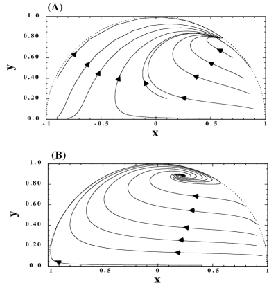
Figure 1: The phase plane for a standard scalar field corresponding to $Q=0.6$ [panel (A)] and $Q=4.0$ [panel (B)] for $\lambda=1.5$, $w_{m}=0$ and $c=1$. The late-time attractor corresponds to a stable node for $Q=0.6$ and a stable spiral for $Q=4.0$. The dotted curve is $x^{2}+y^{2}=1$, which characterizes the border of the allowed region ($\Omega_{\varphi}=1$).

III.2.2 Phantom field $(\epsilon=-1)$

Name	Stability	Acceleration	Existence
(a)	Saddle point for $Q(Q+\lambda)<(3/2)(1-w_{m}^{2})$	$Q^{2}>(1-w_{m})(1+3w_{m})/2$	No if the condition $0\leq\Omega_{\varphi}\leq 1$
	Stable node for $Q(Q+\lambda)>(3/2)(1-w_{m}^{2})$		is imposed
(c)	Stable node	All values	All values
(d)	Saddle	Acceleration for $Q>\lambda(1+3w_{m})/2$	$Q(Q+\lambda)>(3/2)(1-w_{m}^{2})$

Table 3: The conditions for stability & acceleration & existence for a phantom scalar field ($\epsilon=-1$). We consider the situation with positive values of $Q$ and $\lambda$.

Figure 2: Phase plane for a phantom-type scalar field ($\epsilon=-1$) for $Q=3/4$, $\lambda=1$, $w_{m}=0$ and $c=1$. The point A is a stable fixed point (c), whereas the point B is the fixed point (a) corresponding to a saddle. All trajectories approach the point A, which gives $w_{\rm eff}=-4/3$ and $\Omega_{\varphi}=1$. We also show the border of the allowed range ($-1\leq x^{2}-y^{2}\leq 0$) as dotted curves.

Figure 3: Phase plane for a phantom-type scalar field ($\epsilon=-1$) corresponding to $Q=3/2$, $\lambda=2$, $w_{m}=0$ and $c=1$. The point A is a stable fixed point (c), whereas the point B is the fixed point (a) corresponding to a stable node. The point C is the fixed point (d) corresponding to a saddle. In this case the trajectories approach either the point A or B, depending on the initial conditions of $x$ and $y$. The border of the allowed range is the same as in Fig. 2.

The fixed points (b) and (c) do not exist for the phantom field.

• Point (a):

  In this case $\mu_{1}$ is always negative, whereas $\mu_{2}$ can be either positive or negative depending the values of $Q$ and $\lambda$. Then this point is a saddle for $Q(Q+\lambda)<(3/2)(1-w_{m}^{2})$ and a stable node for $Q(Q+\lambda)>(3/2)(1-w_{m}^{2})$. However, since $\Omega_{\varphi}=-2Q^{2}/3(1-w_{m})<0$ for $0\leq w_{m}<1$, the fixed point (a) is not physically meaningful.

• Point (c):

  Since both $\mu_{1}$ and $\mu_{2}$ are negative independent of the values of $\lambda$ and $Q$, the point (c) is a stable node.

• Point (d):

  From the condition $y^{2}>0$, we require that $2Q(Q+\lambda)>3(1-w_{m}^{2})$ for the existence of the critical point (d). Under this condition we find that $\mu_{1}<0$ and $\mu_{2}>0$. Therefore the point (d) corresponds to a saddle.

The properties of the critical points are summarized in Table III. The scaling solution becomes always unstable for phantom. Therefore one can not construct a coupled dark energy scenario in which the present value of $\Omega_{\varphi}$ ($\simeq 0.7$) is a late-time attractor. This property is different from the case of an ordinary field in which scaling solutions can be stable fixed points. The only viable stable attractor for phantom is the fixed point (c), giving the dark energy dominated universe ($\Omega_{\varphi}=1$) with an equation of state $w_{\varphi}=-1-\lambda^{2}/3<-1$.

In Figs. 2 and 3 we plot the phase plane for two different cases. Figure 2 corresponds to $Q=3/4$, $\lambda=1$, $w_{m}=0$ and $c=1$. In this case the fixed point (a) is saddle, whereas the point (d) does not exist. It is clear from Fig. 2 that the fixed point (c) is a global attractor. We also note that the allowed range in the phase plane corresponds to $-1\leq x^{2}-y^{2}\leq 0$, which comes from the condition $0\leq\Omega_{\varphi}\leq 1$. The saddle point (a) exists outside of this region. Figure 3 corresponds to $Q=3/2$, $\lambda=2$, $w_{m}=0$ and $c=1$. In this case the fixed point (a) is a stable node, whereas there exists a saddle point (d). In Fig. 3 we find that the fixed points (a) and (d) are actually stable nodes, although the point (a) is not physically meaningful. Compared to Fig. 2, the critical point (d) newly appears, but this is not a late-time attractor. It is worth mentioning that numerical results agree very well with our analytic estimation for the stability analysis about critical points.

IV Dilatonic ghost condensate

It was pointed out in Ref. UV that at the quantum level a phantom field is plagued by a vacuum instability associated with the production of ghosts and photon pairs. We recall that the phantom field is characterised by a negative value of the quantity: $p_{X}\equiv\partial p/\partial X$. One can consider a scenario which avoids the problem of quantum instability by adding higher-order derivative terms that stabilize the vacuum so that $p_{X}$ becomes positive Arkani . In the context of low-energy effective string theory one may consider the following Lagrangian that involves a dilatonic higher-order term scorre :

$$p=-X+ce^{\lambda\varphi}X^{2}\,,$$ (34)

where $c$ and $\lambda$ are both positive. The application of this scenario to dark energy was done in Ref. PT , but the stability of critical points was not studied.

We obtain the pressure density $(\ref{gcon})$ by choosing the function

$$g(Y)=-1+cY\,,$$ (35)

in Eq. (5). Then Eqs. (10) and (11) yield

$$\frac{{\rm d}x}{{\rm d}N} = \frac{3}{2}x\left[1+w_{m}+(1-w_{m})x^{2}(-1+cY)-2cw_{m}x^{2}Y\right]$$ (36)

$$+\frac{1}{1-6cY}\left[3(-1+2cY)x+\frac{3\sqrt{6}}{2}\lambda cx^{2}Y+\frac{\sqrt{6}Q}{2}\left\{1+x^{2}(1-3cY)\right\}\right]\,,$$

$$\frac{{\rm d}y}{{\rm d}N} = -\frac{\sqrt{6}}{2}\lambda xy+\frac{3}{2}y\left[1+w_{m}+(1-w_{m})x^{2}(-1+cY)-2cw_{m}x^{2}Y\right]\,.$$ (37)

By Eqs. (13) and (14) we find

$$\Omega_{\varphi}=x^{2}(-1+3cY)\,,~{}~{}~{}w_{\varphi}=\frac{-1+cY}{-1+3cY}\,,~{}~{}~{}w_{\rm eff}=w_{m}-(1-w_{m})x^{2}+(1-3w_{m})cx^{2}Y\,.$$ (38)

The stability of quantum fluctuations is ensured for $p_{X}+2Xp_{XX}>0$ and $p_{X}\geq 0$ PT , which correspond to the condition $cY\geq 1/2$. In this case one has $w_{\varphi}\geq-1$ by Eq. (38), which means that the presence of the term $e^{\lambda\varphi}X^{2}$ leads to the stability of vacuum at the quantum level.

IV.1 Fixed points

Setting ${\rm d}X/{\rm d}N=0$ and ${\rm d}Y/{\rm d}N=0$ in Eqs. (36) and (37), we obtain

$$y^{2}=-\frac{3cx^{3}[4-\sqrt{6}(Q+\lambda)x]}{\sqrt{6}x(\lambda x-\sqrt{6})+\sqrt{6}Q(1+x^{2})}\,,~{}~{}~{}~{}y^{2}=\frac{3c(3w_{m}-1)x^{4}}{3(1+w_{m})-3(1-w_{m})x^{2}-\sqrt{6}\lambda x}\,.$$ (39)

Combining these relations, we get four critical points presented in Table 4. The point (a) corresponds to $x=0$ and $y=0$, in which case one has $Y\to\infty$ by Eq. (39). Since we require the condition $w_{m}\leq-1$ in order to satisfy $0\leq\Omega_{\varphi}\leq 1$, this is not a physically meaningful solution.

The points (b) and (c) correspond to the dark-energy dominated universe with $\Omega_{\varphi}=1$. Therefore these points exist irrespective of the presence of the coupling $Q$. In Table 4 the functions $f_{\pm}(\lambda)$ are defined by

$$f_{\pm}(\lambda)\equiv 1\pm\sqrt{1+16/(3\lambda^{2})}\,.$$ (40)

Since one has $w_{\rm eff}=w_{\varphi}=(-1+cY)/(-1+3cY)$ for the points (b) and (c), the condition for an accelerated expansion, $w_{\rm eff}<-1/3$, gives $cY<2/3$. We note that $w_{\rm eff}<-1$ for $cY<1/2$ and $w_{\rm eff}>-1$ otherwise. The former case corresponds to the phantom equation of state, whereas the latter belongs to the case in which the system is stable at the quantum level. The parameter range of $Y$ for the point (b) is $1/3<cY<1/2$, which means that the field $\varphi$ behaves as a phantom. In this case the universe exhibits an acceleration for any value of $\lambda$ and $Q$. The point (c) belongs to the parameter range given by $1/2<cY<\infty$. The condition for an accelerated expansion corresponds to $\lambda^{2}f_{+}(\lambda)<8/3$, which gives $\lambda\lesssim 0.817$. In the limit $\lambda\to 0$ we have $cY\to 1/2$, $\Omega_{\varphi}\to 1$ and $w_{\rm eff}=w_{\varphi}\to-1$ for both points (b) and (c). The $\lambda=0$ case is the original ghost condensate scenario proposed in Ref. Arkani , i.e., $p=-X+X^{2}$, in which case one has an equation of state of cosmological constant ($w_{\varphi}=-1$).

The point (d) corresponds to a scaling solution. Since the effective equation of state is given by $w_{\rm eff}=(w_{m}\lambda-Q)/(\lambda+Q)$, the universe accelerates for $Q>\lambda(1+3w_{m})/2$. The requirement of the conditions $0\leq\Omega_{\varphi}\leq 1$ and $Y=x^{2}/y^{2}>0$ places constraints on the values of $Q$ and $\lambda$. For the non-relativistic dark matter ($w_{m}=0$) with positive coupling ($Q>0$), we have the following constraint

$$\frac{1}{2}\left[\sqrt{9Q^{2}+12}-5Q\right]<\lambda<\frac{1}{Q}-Q\,.$$ (41)

This implies that $Q$ needs to be smaller than 1 for positive $\lambda$.

Name	$x$	$cY$	$\Omega_{\varphi}$	$w_{\varphi}$	$w_{\rm eff}$
(a)	0	$\infty$	$\frac{3(w_{m}+1)}{3w_{m}-1}$	1/3	$-1$
(b)	$-\frac{\sqrt{6}\lambda f_{+}(\lambda)}{4}$	$\frac{1}{2}+\frac{\lambda^{2}f_{-}(\lambda)}{16}$	1	$\frac{-8+\lambda^{2}f_{-}(\lambda)}{8+3\lambda^{2}f_{-}(\lambda)}$	$\frac{-8+\lambda^{2}f_{-}(\lambda)}{8+3\lambda^{2}f_{-}(\lambda)}$
(c)	$-\frac{\sqrt{6}\lambda f_{-}(\lambda)}{4}$	$\frac{1}{2}+\frac{\lambda^{2}f_{+}(\lambda)}{16}$	1	$\frac{-8+\lambda^{2}f_{+}(\lambda)}{8+3\lambda^{2}f_{+}(\lambda)}$	$\frac{-8+\lambda^{2}f_{+}(\lambda)}{8+3\lambda^{2}f_{+}(\lambda)}$
(d)	$\frac{\sqrt{6}(1+w_{m})}{2(\lambda+Q)}$	$\frac{3(1-w_{m}^{2})-2Q(\lambda+Q)}{3(1-3w_{m})(1+w_{m})}$	$\frac{3(1+w_{m})[1+w_{m}-Q(\lambda+Q)]}{(\lambda+Q)^{2}(1-3w_{m})}$	$\frac{3(1+w_{m})w_{m}-Q(\lambda+Q)}{3(1+w_{m})-3Q(\lambda+Q)}$	$\frac{w_{m}\lambda-Q}{\lambda+Q}$

Table 4: The critical points for the ghost condensate model (34). Here the functions $f_{\pm}(\lambda)$ are defined by Eq. (40).

IV.2 Stability around fixed points

The elements of the matrix ${\cal M}$ for perturbations $u$ and $v$ are given by

$$a_{11} = \frac{3}{2}\left[1+w_{m}-3(1-w_{m})x_{c}^{2}+5c(1-3w_{m})x_{c}^{2}Y_{c}\right]+\frac{-3+\sqrt{6}x_{c}Q+18cY_{c}+6\sqrt{6}c(\lambda-Q)x_{c}Y_{c}}{1-6cY_{c}}$$ (42)

$$+\frac{12cY_{c}}{x_{c}(-1+6cY_{c})^{2}}\left[3(-1+2cY_{c})x_{c}+\frac{3\sqrt{6}}{2}\lambda cx_{c}^{2}Y_{c}+\frac{\sqrt{6}Q}{2}\left\{1-x_{c}^{2}(-1+3cY_{c})\right\}\right]\,,$$

$$a_{12} = -3c(1-3w_{m})x_{c}^{2}Y_{c}^{3/2}-\frac{\sqrt{6}c}{1-6cY_{c}}Y_{c}^{3/2}\left\{2\sqrt{6}+3x_{c}(\lambda-Q)\right\}$$ (43)

$$-\frac{12cY_{c}}{y_{c}(-1+6cY_{c})^{2}}\left[3(-1+2cY_{c})x_{c}+\frac{3\sqrt{6}}{2}\lambda cx_{c}^{2}Y_{c}+\frac{\sqrt{6}Q}{2}\left\{1-x_{c}^{2}(-1+3cY_{c})\right\}\right]\,,$$

$$a_{21} = 3y_{c}\left[-(1-w_{m})x_{c}+2c(1-3w_{m})x_{c}Y_{c}\right]-\frac{\sqrt{6}}{2}\lambda y_{c}\,,$$ (44)

$$a_{22} = \frac{3}{2}\left[1+w_{m}-(1-w_{m})x_{c}^{2}-c(1-3w_{m})x_{c}^{2}Y_{c}\right]-\frac{\sqrt{6}}{2}\lambda x_{c}\,.$$ (45)

Since the expression of the matrix elements is rather complicated, the eigenvalues of ${\cal M}$ are not simply written unlike the case of Sec. III. However we can numerically evaluate $\mu_{1}$ and $\mu_{2}$ and investigate the stability of fixed points.

• Point (a):

  In this case the component $a_{12}$ diverges, which means that this point is unstable in addition to the fact $\Omega_{\varphi}$ does not belong to the range $0\leq\Omega_{\varphi}\leq 1$ for plausible values of $w_{m}$.

• Point (b):

  We numerically evaluate the eigenvalues $\mu_{1}$ and $\mu_{2}$ for $w_{m}=0$, $c=1$ and find that the point (b) is either a stable spiral or a stable node. When $Q\lesssim 10$ the determinant of the matrix ${\cal M}$ is negative with negative real parts of $\mu_{1}$ and $\mu_{2}$, which means that the point (b) is a stable spiral. In the case of $Q\gtrsim 10$, the determinant is positive with negative $\mu_{1}$ and $\mu_{2}$ if $\lambda$ is smaller than a value $\lambda_{*}(Q)$, thereby corresponding to a stable node. Here $\lambda_{*}(Q)$ depends on the value $Q$. When $\lambda>\lambda_{*}(Q)$ and $Q\gtrsim 10$, the point (b) is a stable spiral.

• Points (c) & (d):

  It would be convenient to discuss the stability of these critical points together as there exists an interesting relation between them. We shall consider the case of $w_{m}=0$ and $c=1$.

  For the point (c) we have numerically found that $\mu_{2}$ is always negative irrespective of the values of $Q$ and $\lambda$. Our analysis shows that there exists a critical value $\bar{\lambda}_{*}(Q)$ such that $\mu_{1}$ is negative for $\lambda<\bar{\lambda}_{*}(Q)$ and becomes positive for $\lambda>\bar{\lambda}_{*}(Q)$. The critical value of $\lambda$ can be computed by demanding $(a_{11}a_{22}-a_{12}a_{21})=0$, which leads to

  $$\bar{\lambda}_{*}(Q)=\frac{1}{2}\left[\sqrt{9Q^{2}+12}-5Q\right]\,.$$ (46)

  We conclude that in the region specified by $0<\lambda<\bar{\lambda}_{*}(Q)$, the critical point (c) is a stable node which becomes a saddle as we move out of this region [$\lambda>\bar{\lambda}_{*}(Q)$].

  For the point (d) the second eigenvalue $\mu_{2}$ is negative or ${\rm Re}\,(\mu_{2})<0$ for all values of $Q$ and $\lambda$. Meanwhile the first eigenvalue exhibits an interesting behavior. We recall that the allowed domain for the existence of the point (d) lies outside the region of stability for the point (c), see Eq. (41). If we extend it to the region $\lambda<\bar{\lambda}_{*}(Q)$, we find that point (d) is a saddle in this domain ($\mu_{1}>0$ and $\mu_{2}<0$). The critical value of ${\lambda}$, at which $\mu_{1}$ for the point (d) vanishes, exactly coincides with $\bar{\lambda}_{*}(Q)$ given by Eq. (46). As we move out of the domain of stability for the point (c), the critical point (d) becomes a stable node as $\mu_{1}<0$ in this case. We numerically find there exists a second critical value $\tilde{\lambda}_{**}(Q)~{}(>\bar{\lambda}_{*}(Q))$ at which the determinant ${\cal D}$ of the system vanishes such that $\mu_{1}<0$ for $\bar{\lambda}_{*}(Q)<\lambda<\tilde{\lambda}_{**}(Q)$ and ${\rm Re}\,(\mu_{1})<0$ for $\lambda>\tilde{\lambda}_{**}(Q)$. To have an idea of orders of magnitudes, let us quote some numerical values of $\bar{\lambda}_{*}(Q)$ and $\tilde{\lambda}_{**}(Q)$, for instance $\tilde{\lambda}_{**}(Q)=2.06,~{}1.15$; $\bar{\lambda}_{*}(Q)=1.26,~{}0.64$ for $Q=0.2,0.5$ respectively. The stability of (c) & (d) can be briefly summarised as follows. The point (c) is a stable node whereas the point (d) is a saddle for $0<\lambda<\bar{\lambda}_{*}(Q)$. The point (c) becomes a saddle for $\lambda>\lambda_{*}(Q)$. In the region characterised by $\bar{\lambda}_{*}(Q)<\lambda<\tilde{\lambda}_{**}(Q)$, the critical point (d) is a stable node but a stable spiral for $\lambda>\tilde{\lambda}_{**}(Q)$.

We summarize the property of fixed points in Table 5. Although the point (b) is always stable at the classical level, this corresponds to a phantom equation of state ($w_{\varphi}<-1$). Therefore this is plagued by the instability of vacuum at the quantum level, whereas the point (c) is free from such a quantum instability. The scaling solution (d) also gives rise to an equation of state $w_{\varphi}>-1$ as can be checked by the expression of $w_{\varphi}$ in Table 4. When the point (c) is stable we find that the point (d) is unstable, and vice versa. Therefore the final viable attractor is described by a dark energy dominant universe with $\Omega_{\varphi}=1$ [case (c)] or by a scaling solution with $0<\Omega_{\varphi}={\rm const}<1$ [case (d)].

Name	Stability	Acceleration	Existence
(a)	Unstable	All values	$w_{m}\leq-1$
(b)	Stable spiral or stable node	All values	All values
(c)	Stable node or saddle	$\lambda<0.817$	All values
(d)	Stable node or stable spiral or saddle	$Q>\lambda(1+3w_{m})/2$	$[(9Q^{2}+12)^{1/2}-5Q]/2<\lambda<1/Q-Q$ for $w_{m}=0$

Table 5: The conditions for stability & acceleration & existence for the ghost condensate model (34).

In Fig. 4 we plot the phase plane for $Q=0.5$ and $\lambda=0.4$. In this case the point (c) is a saddle, whereas the point (d) is a stable node. By using the condition $0\leq\Omega_{\varphi}\leq 1$ in Eq. (38), we find that $x$ and $y$ are constrained to be in the range: $3cx^{4}/(1+x^{2})\leq y^{2}\leq 3cx^{2}$. We also obtain the condition, $y^{2}\leq 2cx^{2}$, if the stability of quantum fluctuations is taken into account PT . When $x$ and $y$ are initially smaller than of order unity with positive $x$, the trajectories tend to approach the line $y=\sqrt{6c}x$ on which the speed of sound, $c_{s}\equiv\sqrt{p_{X}/\rho_{X}}$, diverges PT . Therefore these cases are physically unrealistic. Meanwhile when initial conditions of $x$ and $y$ are not much smaller than of order unity, the solutions approach the stable point (d) provided that $x$ is positive (see Fig. 4). When $x$ and $y$ are much smaller than 1 during matter dominant era, it is difficult to reach the critical point (d) for constant $Q$. If the coupling $Q$ rapidly grows during the transition to scalar field dominated era, it is possible to approach the scaling solution (d) PT .

If the initial value of $x$ is negative, the trajectories approach the stable point (b). In this case we numerically found that the solutions do not cross the lines $y=\sqrt{6c}|x|$ even for the initial values of $|x|$ much smaller than unity. The final attractor point (b) corresponds to the phantom-dominant universe with $\Omega_{\varphi}=1$.

Figure 4: Phase plane analysis in the dilatonic ghost condensate case for $Q=0.5$ and $\lambda=0.8$ with $w_{m}=0$ and $c=1$. In this case there exist two stable points (b) $(x,y)=(-1.98,3.07)$ and (d) $(x,y)=(0.94,1.25)$. The curves (i), (ii) and (iii) correspond to $y^{2}=3cx^{4}/(1+x^{2})$, $y^{2}=3cx^{2}$ and $y^{2}=6cx^{2}$, respectively.

V Tachyon and phantom tachyon

The Lagrangian of a tachyon field is given, in general, by Sen

$$p=-V(\phi)\sqrt{1-\epsilon\dot{\phi}^{2}}\,,$$ (47)

where $\epsilon=+1$. Here we allowed the possibility of a phantom tachyon ($\epsilon=-1$) Hao . We note that there are many works in which the dynamics of tachyon is investigated in a cosmological context tachyon . The potential corresponding to scaling solutions is the inverse power-law type, i.e., $V(\phi)\propto\phi^{-2}$. If we choose the function $g(Y)$ as

$$g(Y) = -c\sqrt{1-2\epsilon Y}/Y\,,$$ (48)

the Lagrangian (5) yields $p=-ce^{-\lambda\varphi}\sqrt{1-2\epsilon Y}$. With a suitable field redefinition given by $\phi=(2/\lambda)e^{{\lambda\varphi}/2}$, we obtain the tachyon Lagrangian (47) with an inverse square potential: $V(\phi)=4c/(\lambda^{2}\phi^{2})$. Note that we are considering positive $c$.

We shall introduce a new variable $\tilde{x}$ which is defined by $\tilde{x}^{2}\equiv\dot{\phi}^{2}/2=Y$. Then $x$ and $\tilde{x}$ are now related as $x=\tilde{x}y$. Noting that

$$g(Y)+5Yg^{\prime}(Y)+2Y^{2}g^{\prime\prime}(Y) = \frac{c\epsilon}{(1-2\epsilon Y)^{3/2}}\,,$$ (49)

we obtain the following equations by using Eqs. (10) and (11):

$$\frac{{\rm d}\tilde{x}}{{\rm d}N} = -(1-2\epsilon\tilde{x}^{2})\left[3\tilde{x}-\frac{\sqrt{6}\lambda y}{2\epsilon}+\frac{\sqrt{6}Q}{2c\epsilon y}(\sqrt{1-2\epsilon\tilde{x}^{2}}-cy^{2})\right]\,,$$ (50)

$$\frac{{\rm d}y}{{\rm d}N} = -\frac{\sqrt{6}}{2}\lambda\tilde{x}y^{2}+\frac{3y}{2}\left[\gamma-\frac{cy^{2}}{\sqrt{1-2\epsilon\tilde{x}^{2}}}(\gamma-2\epsilon\tilde{x}^{2})\right]\,,$$ (51)

where

$$\gamma\equiv 1+w_{m}\,.$$ (52)

Eqs. (13) and (14) give

$$\Omega_{\varphi}=\frac{cy^{2}}{\sqrt{1-2\epsilon\tilde{x}^{2}}}\,,~{}~{}~{}w_{\varphi}=2\epsilon\tilde{x}^{2}-1\,,~{}~{}~{}w_{\rm eff}=w_{m}-\frac{cy^{2}(1+w_{m}-2\epsilon\tilde{x}^{2})}{\sqrt{1-2\epsilon\tilde{x}^{2}}}\,.$$ (53)

V.1 Fixed points

When we discuss fixed points in the tachyon model, it may be convenient to distinguish between two cases: $Q=0$ and $Q\neq 0$. We note that the fixed points were derived in Ref. AL ; CGST for $Q=0$ and $\epsilon=+1$.

V.1.1 $Q=0$

We summarize the fixed points in Table 6 for $Q=0$. The point (a) is a fluid-dominant solution ($\Omega_{m}\to 1$) with an effective equation of state, $w_{\rm eff}=w_{m}$. Then the accelerated expansion does not occur unless $w_{m}$ is less than $-1/3$. The points (b1) and (b2) are the kinematic dominant solution whose effective equation of state corresponds to a dust. This does not exist in the case of phantom tachyon. The point (c) is a scalar-field dominant solution that gives an accelerated expansion at late times for $\lambda^{2}y_{c}^{2}/(3\epsilon)<2/3$, where $y_{c}$ is defined by

$$y_{c}\equiv\left[\frac{-\lambda^{2}\pm\sqrt{\lambda^{4}+36c^{2}}}{6\epsilon c^{2}}\right]^{1/2}\,.$$ (54)

This condition translates into $\lambda^{2}<2\sqrt{3}c$ for $\epsilon=+1$. In Eq. (54) the plus sign corresponds to $\epsilon>0$, whereas the minus sign to $\epsilon<0$. Note that phantom tachyon gives an effective equation of state $w_{\rm eff}$ that is smaller than $-1$. The points (d1) and (d2) correspond to scaling solutions in which the energy density of the scalar field decreases proportionally to that of the perfect fluid ($w_{\varphi}=w_{m}$). The existence of this solution requires the condition $w_{m}<0$ as can be seen in the expression of $\Omega_{\varphi}$. We note that the fixed points (d1) and (d2) do not exist for phantom tachyon unless the background fluid behaves as phantom ($w_{m}<-1$).

Name	$\tilde{x}$	$y$	$\Omega_{\varphi}$	$w_{\varphi}$	$w_{\rm eff}$
(a)	0	0	0	$-1$	$w_{m}$
(b1)	$\frac{1}{\sqrt{2\epsilon}}$	0	1	0	0
(b2)	$-\frac{1}{\sqrt{2\epsilon}}$	0	1	0	0
(c)	$\frac{\lambda y_{c}}{\sqrt{6}\epsilon}$	$y_{c}$	1	$\frac{\lambda^{2}y_{c}^{2}}{3\epsilon}-1$	$\frac{\lambda^{2}y_{c}^{2}}{3\epsilon}-1$
(d1)	$(\gamma/2\epsilon)^{1/2}$	$\frac{\sqrt{3\epsilon\gamma}}{\lambda}$	$\frac{3c\epsilon\gamma}{\lambda^{2}\sqrt{1-\gamma}}$	$w_{m}$	$w_{m}$
(d2)	$-(\gamma/2\epsilon)^{1/2}$	$-\frac{\sqrt{3\epsilon\gamma}}{\lambda}$	$\frac{3c\epsilon\gamma}{\lambda^{2}\sqrt{1-\gamma}}$	$w_{m}$	$w_{m}$

Table 6: The critical points for the tachyon model (47) with $Q=0$. Here $y_{c}$ is defined by Eq. (54). The points (b) and (d) do not exist for the phantom tachyon ($\epsilon<0$).

V.1.2 $Q\neq 0$

Let us next discuss the case with $Q\neq 0$. The critical points are summarized in Table 7. We first note that the fixed point $(x,y)=(0,0)$ disappears in the presence of the coupling $Q$. The points (b) and (c) appear as is similar to the case $Q=0$. While (b1) and (b2) do not exist for phantom tachyon, the point (c) exists both for $\epsilon>0$ and $\epsilon<0$.

The point (d) [$(x_{i},y_{i})$] corresponds to scaling solutions, whose numbers of solutions depend on the value of $w_{m}$. $y_{i}$ are related with $x_{i}$ through the relation $y_{i}=3\gamma/[\sqrt{6}(\lambda+Q)\tilde{x}_{i}]$. Here $x_{i}$ satisfy the following equation

$$\frac{\gamma-2\epsilon\tilde{x}_{i}^{2}}{\tilde{x}_{i}^{2}\sqrt{1-2\epsilon\tilde{x}_{i}^{2}}}=\frac{2Q(\lambda+Q)}{3(1+w_{m})c}\,.$$ (55)

We note that only positive $x_{i}$ are allowed for $\lambda>0$, since $y_{i}$ is positive definite. If we introduce the quantity $\xi\equiv\sqrt{-w_{\varphi}}=\sqrt{1-2\epsilon\tilde{x}_{i}^{2}}$, we find

$$f(\xi)\equiv\frac{\xi^{2}+w_{m}}{\xi(1-\xi^{2})}=\frac{Q(Q+\lambda)}{3c\epsilon(1+w_{m})}\,.$$ (56)

The behavior of the function $f(\xi)$ is different depending on the value of $w_{m}$. We note that $\lambda$ is related with the slope of the potential as $\lambda=-V_{\phi}/V^{3/2}$ CGST , which means that $\lambda>0$ for the inverse power-law potential: $V(\phi)=M^{2}\phi^{-2}$. Then the r.h.s. of Eq. (56) is positive for $\epsilon>0$ and negative otherwise. The allowed range of $\xi$ is $0<\xi<1$ for $\epsilon>0$ and $\xi>1$ for $\epsilon<0$. We can classify the situation as follows.

• $w_{m}>0$:

  The function $f(\xi)$ goes to infinity for $\xi\to 0+0$ and $\xi\to 1-0$. It has a minimum at $\xi=\xi_{M}$ with $0<\xi_{M}<1$. Here $\xi_{M}$ is defined by $\xi_{M}^{2}\equiv[-(1+3w_{m})+\sqrt{(1+w_{m})(1+9w_{m})}]/2$. Then for $\epsilon>0$, there exist two solutions for Eq. (56) provided that $Q(Q+\lambda)/(3c\epsilon(1+w_{m}))>f(\xi_{M})$. The function $f(\xi)$ has a dependence $f(\xi)\to-\infty$ for $\xi\to 1+0$ and $f(\xi)\to 0$ for $\xi\to+\infty$. Then for $\epsilon<0$, there exists one scaling solution for Eq. (56).

• $w_{m}=0$:

  In this case we can analytically derive the solution for Eq. (56). The function $f(\xi)$ is zero at $\xi=0$ and monotonically increases toward $+\infty$ as $\xi\to 1-0$. Then we have one solution for Eq. (56) if $\epsilon>0$. The function $f(\xi)$ has a dependence $f(\xi)\to-\infty$ for $\xi\to 1+0$ and $f(\xi)\to 0$ for $\xi\to+\infty$. This again shows the existence of one solution for Eq. (56) if $\epsilon<0$. The solutions for Eq. (56) are given by $\xi=[-1+\sqrt{1+4A^{2}}]/2A$ for $\epsilon=+1$ and $\xi=[1+\sqrt{1+4A^{2}}]/2A$ for $\epsilon=-1$, where $A\equiv Q(Q+\lambda)/(3c(1+w_{m}))$. Then we obtain the following fixed points together with the equation of state $w_{\varphi}$:

  $$\tilde{x}_{c}=\frac{\sqrt{3}\sqrt{c(-3c+\sqrt{9c^{2}+4Q^{2}(\lambda+Q)^{2}})}}{2Q(\lambda+Q)}\,,$$ (57)

  $$y_{c}=\frac{\sqrt{6}Q}{\sqrt{3}\sqrt{c(-3c+\sqrt{9c^{2}+4Q^{2}(\lambda+Q)^{2}}})}\,,$$ (58)

  $$w_{\varphi}=-\frac{9c^{2}}{4Q^{2}(Q+\lambda)^{2}}\left[\sqrt{1+\frac{4Q^{2}(Q+\lambda)^{2}}{9c^{2}}}-1\right]^{2}\,,$$ (59)

  for $\epsilon=+1$ and

  $$\tilde{x}_{c}=\frac{\sqrt{3}\sqrt{c(3c+\sqrt{9c^{2}+4Q^{2}(\lambda+Q)^{2}})}}{2Q(\lambda+Q)}\,,$$ (60)

  $$y_{c}=\frac{\sqrt{6}Q}{\sqrt{3}\sqrt{c(3\ c+\sqrt{9c^{2}+4Q^{2}(\lambda+Q)^{2}}})}\,,$$ (62)

  $$w_{\varphi}=-\frac{9c^{2}}{4Q^{2}(Q+\lambda)^{2}}\left[\sqrt{1+\frac{4Q^{2}(Q+\lambda)^{2}}{9c^{2}}}+1\right]^{2}\,,$$

  for $\epsilon=-1$.

  For ordinary tachyon one has $\tilde{x}_{c}\to 1/\sqrt{2}$, $y_{c}\to\sqrt{3}/(\lambda+Q)$, $w_{\varphi}\to 0$ as $Q\to 0$ and $\tilde{x}_{c}\to 0$, $y_{c}\to 1/\sqrt{c}$, $w_{\varphi}\to-1$ as $Q\to+\infty$. There is a critical value $Q_{*}(\lambda)$ which gives the border of acceleration and deceleration, i.e., the accelerated expansion occurs for $Q>Q_{*}(\lambda)$. For phantom tachyon we obtain $\tilde{x}_{c}\to\infty$, $y_{c}\to 0$, $w_{\varphi}\to-\infty$ as $Q\to 0$ and $\tilde{x}_{c}\to 0$, $y_{c}\to 1/\sqrt{c}$, $w_{\varphi}\to-1$ as $Q\to+\infty$. Thus the presence of the coupling $Q$ can lead to an accelerated expansion.

• $w_{m}<0$:

  The function $f(\xi)$ is zero at $\xi=\sqrt{-w_{m}}$. It monotonically increases toward $+\infty$ as $\xi\to 1-0$ in the region $\sqrt{-w_{m}}<\xi<1$. This means that we have one solution for Eq. (56) if $\epsilon>0$. The function $f(\xi)$ has a dependence $f(\xi)\to-\infty$ for $\xi\to 1+0$ and $f(\xi)\to 0$ for $\xi\to+\infty$, which shows the existence of one solution for Eq. (56) if $\epsilon<0$. Note, however, that the $w_{m}<0$ case is not realistic.

Name	$\tilde{x}$	$y$	$\Omega_{\varphi}$	$w_{\varphi}$	$w_{\rm eff}$
(b1)	$\frac{1}{\sqrt{2\epsilon}}$	0	1	0	0
(b2)	$-\frac{1}{\sqrt{2\epsilon}}$	0	1	0	0
(c)	$\frac{\lambda y_{c}}{\sqrt{6}\epsilon}$	$y_{c}$	1	$\frac{\lambda^{2}y_{c}^{2}}{3\epsilon}-1$	$\frac{\lambda^{2}y_{c}^{2}}{3\epsilon}-1$
(d)	$\tilde{x}_{i}$	$\frac{3\gamma}{\sqrt{6}(\lambda+Q)\tilde{x}_{i}}$	$\frac{3c\gamma^{2}}{2(\lambda+Q)^{2}\tilde{x}_{i}^{2}\sqrt{1-2\epsilon\tilde{x}_{i}^{2}}}$	$2\epsilon\tilde{x}_{i}^{2}-1$	$w_{m}-\frac{cy_{i}^{2}(1+w_{m}-2\epsilon\tilde{x}_{i}^{2})}{\sqrt{1-2\epsilon\tilde{x}_{i}^{2}}}$

Table 7: The critical points for the tachyon model with $Q\neq 0$. Here $y_{c}$ is defined by Eq. (54). $\tilde{x}_{i}$ are the solutions of Eq. (55). The critical points (b1) and (b2) do not exist for the phantom tachyon ($\epsilon<0$). The numbers of the point (d) depend on the value of $w_{m}$.

V.2 Stability

The components of the matrix ${\cal M}$ are

$$a_{11} = -3+18\,\epsilon\tilde{x}_{c}^{2}-2\sqrt{6}(\lambda+Q)\tilde{x}_{c}y_{c}+\frac{3\sqrt{6}Q\tilde{x}_{c}}{cy_{c}}\,\sqrt{1-2\epsilon\tilde{x}_{c}^{2}}\,,$$ (63)

$$a_{12} = (1-2\epsilon\tilde{x}_{c}^{2})\left[\frac{\sqrt{6}(\lambda+Q)}{2\epsilon}+\frac{\sqrt{6}Q}{2c\epsilon y_{c}^{2}}\sqrt{1-2\epsilon\tilde{x}_{c}^{2}}\right]\,,$$ (64)

$$a_{21} = -\frac{\sqrt{6}}{2}\lambda y_{c}^{2}-\frac{3c\epsilon\tilde{x}_{c}y_{c}^{3}(\gamma-2\epsilon\tilde{x}_{c}^{2})}{(1-2\epsilon\tilde{x}_{c}^{2})^{3/2}}+\frac{6c\epsilon\tilde{x}_{c}y_{c}^{3}}{\sqrt{1-2\epsilon\tilde{x}_{c}^{2}}}\,,$$ (65)

$$a_{22} = -\sqrt{6}\lambda\,\tilde{x}_{c}y_{c}+\frac{3}{2}\gamma-\frac{9cy_{c}^{2}(\gamma-2\epsilon\tilde{x}_{c}^{2})}{2\sqrt{1-2\epsilon\tilde{x}_{c}^{2}}}\,.$$ (66)

Hereafter we shall discuss the stability of fixed points for an ordinary tachyon ($\epsilon=+1$) and for a phantom tachyon ($\epsilon=-1$) by evaluating eigenvalues of the matrix ${\cal M}$.

V.2.1 Ordinary tachyon $(\epsilon=+1)$

The stability of fixed points is summarized in Table 8.

• Point (a):

  This point exists only for $Q=0$. The eigenvalues are

  $$\mu_{1}=3\gamma/2\,,~{}~{}~{}\mu_{2}=-3\,.$$ (67)

  Therefore the point (a) is a saddle for $\gamma>0$ and a stable node for $\gamma<0$. Therefore this point is not stable for an ordinary fluid satisfying $\gamma\geq 1$.

• Points (b1) and (b2):

  Since the eigenvalues are

  $$\mu_{1}=6\,,~{}~{}~{}\mu_{2}=9/2-3\gamma\,,$$ (68)

  the points (b1) and (b2) are unstable nodes for $\gamma<3/2$ and saddle points for $\gamma>3/2$.

• Point (c):

  The eigenvalues are

  $$\mu_{1}=-3\gamma+\frac{\lambda(\lambda+Q)}{6c^{2}}\left(\sqrt{\lambda^{4}+36c^{2}}-\lambda^{2}\right)\,,~{}~{}~{}~{}\mu_{2}=-3+\frac{\lambda^{2}}{12c^{2}}\left(\sqrt{\lambda^{4}+36c^{2}}-\lambda^{2}\right)\,.$$ (69)

  The range of $\mu_{2}$ is $-3\leq\mu_{2}<-3/2$. We also find that $\mu_{1}\leq 0$ if

  $$\gamma\geq\gamma_{s}\equiv\frac{\lambda(\lambda+Q)}{18c^{2}}\left(\sqrt{\lambda^{4}+36c^{2}}-\lambda^{2}\right)\,,$$ (70)

  and $\mu_{1}>0$ if $\gamma<\gamma_{s}$. Therefore the point (c) is a stable node for $\gamma\geq\gamma_{s}$ and a saddle point for $\gamma<\gamma_{s}$.

• Point (d):

  When $Q=0$ we obtain $\gamma\leq\gamma_{s}=\lambda^{2}[\sqrt{\lambda^{4}+36c^{2}}-\lambda^{2}]/(18c^{2})$ from the condition $\Omega_{\varphi}\leq 1$. The eigenvalues for $Q=0$ are

  $$\mu_{1,2}=\frac{3}{4}\left[\gamma-2\pm\sqrt{17\gamma^{2}-20\gamma+4+\frac{48c\gamma^{2}}{\lambda^{2}}\sqrt{1-\gamma}}\right]\,,$$ (71)

  which are both negative for $\gamma\leq\gamma_{s}$. Therefore the point (d) is a stable node for $Q=0$.

  This situation changes if we account for the coupling $Q$. In what follows we shall consider the case of a non relativistic dark matter ($w_{m}=0$). The analytic expressions for the eigenvalues are rather cumbersome for general $Q$, but they take simple forms in the large coupling limit ($Q\to+\infty$):

  $$\mu_{1,2}\simeq-3\pm\sqrt{-\frac{3\lambda Q}{c}}\,.$$ (72)

  This demonstrates that the critical point (d) is a stable spiral for large $Q$. In fact we numerically confirmed that the determinant of the matrix ${\cal M}$ changes from positive to negative when $Q$ becomes larger than a critical value $Q_{1}(\lambda)$. This critical value depends on $\lambda$, e.g., $Q_{1}(\lambda=0.1)=37.5$ and $Q_{1}(\lambda=1.0)=3.28$ for $c=1$. When $Q>Q_{1}(\lambda)$ numerical calculations show that the point (d) is a stable spiral for any $\lambda$.

  When $Q<Q_{1}(\lambda)$ we find that both $\mu_{1}$ and $\mu_{2}$ are negative when $Q$ is larger than a critical value $Q_{2}(\lambda)$. Meanwhile $\mu_{1}>0$ and $\mu_{2}<0$ for $Q<Q_{2}(\lambda)$. Here $Q_{2}(\lambda)$ can be analytically derived as

  $$Q_{2}(\lambda)=-\frac{\lambda}{2}+\frac{\sqrt{\lambda^{4}+36c^{2}}}{2\lambda}\,,$$ (73)

  which corresponds to the eigenvalue: $\mu_{1}=0$. For example we have $Q_{2}(\lambda=0.1)=29.95$ and $Q_{2}(\lambda=1.0)=2.54$ for $c=1$. From the above argument the fixed point (d) is a saddle for $Q<Q_{2}(\lambda)$, a stable node for $Q_{2}(\lambda)<Q<Q_{1}(\lambda)$ and a stable spiral for $Q>Q_{1}(\lambda)$.

Name	Stability	Acceleration	Existence
(a)	Saddle point for $\gamma>0$	$\gamma<2/3$	$Q\neq 0$
	Stable node for $\gamma<0$
(b1), (b2)	Unstable node for $\gamma<3/2$	No	All values
	Saddle point for $\gamma>3/2$
(c)	Stable node for $\gamma\geq\gamma_{s}$	$\lambda^{2}<2\sqrt{3}c$	All values
	Saddle point for $\gamma<\gamma_{s}$
(d) [$Q=0$]	Stable node or stable spiral	$\gamma<2/3$	$0\leq\gamma<1$
(d) [$Q\neq 0$]	Stable node or stable spiral or saddle	$Q>\tilde{Q}_{*}(\lambda)$	$\tilde{x}_{i}^{2}(1-2\tilde{x}_{i}^{2})^{1/2}\geq\frac{9c\lambda^{2}}{2(\lambda+Q)^{2}}$

Table 8: The conditions for stability & acceleration & existence for an ordinary tachyon field ($\epsilon=+1$). $\gamma_{s}$ is defined by Eq. (70). $\tilde{Q}_{*}(\lambda)$ depends on $\lambda$.

In the case of $w_{m}=0$, the stability condition (70) for the point (c) corresponds to

$$Q\leq-\frac{\lambda}{2}+\frac{\sqrt{\lambda^{4}+36c^{2}}}{2\lambda}\,.$$ (74)

The r.h.s. completely coincides with $Q_{2}(\lambda)$. This means that the critical point (c) presents a stable node in the region where (d) is a saddle. When $Q>Q_{2}(\lambda)$ the point (d) is stable, whereas (c) is a saddle. Therefore one can not realize the situation in which both (c) and (d) are stable.

In Fig. 5 we plot the evolution of $\Omega_{\varphi}$ and $\Omega_{m}$ for $Q=3.0$ and $\lambda=2.18$. Since $Q_{1}(\lambda)=1.02$ and $Q_{2}(\lambda)=0.67$ in this case, the fixed point (d) is a stable spiral whereas the point (c) is a saddle. In fact the solutions approach the point (d) with oscillations as is clearly seen in Fig. 5. The attractor corresponds to a scaling solution that gives $\Omega_{\varphi}=0.7$ and $\Omega_{m}=0.3$.

Figure 5: The evolution of $\Omega_{\varphi}$ and $\Omega_{m}$ for an ordinary tachyon ($\epsilon=+1$) with $Q=3.0$ and $\lambda=2.18$. The stable attractor in this case is the fixed point (d), giving $\Omega_{\varphi}=0.7$ and $\Omega_{m}=0.3$ asymptotically.

V.2.2 Phantom tachyon $(\epsilon=-1)$

For a phantom tachyon the stability of fixed points exhibits a number of differences compared to an ordinary tachyon.

• Point (a):

  The property of this fixed point is completely the same as in the case of an ordinary tachyon.

• Point (c):

  In this case the calculation of the eigenvalues of the matrix ${\cal M}$ is more involved compared to the point (c) for $\epsilon=+1$, but we numerically find that $\mu_{1}$ and $\mu_{2}$ are both negative for any value of $Q$ and $\lambda$. Then the point (c) is a stable node.

• Point (d):

  In the case of $w_{m}=0$, the critical points are given by Eqs. (60) and (62). In the large coupling limit $Q\to\infty$, the eigenvalues are approximately given by

  $$\mu_{1,2}\simeq-3\pm\sqrt{\frac{3\lambda Q}{c}}\,,$$ (75)

  which means that $\mu_{1}$ is positive and $\mu_{2}$ is negative. Numerically we find that $\mu_{1}>0$ and $\mu_{2}<0$ for any value of $Q$ and $\lambda$. Then the fixed point (d) is always saddle.

From the above argument scaling solutions do not give a viable late-time attractor for the phantom. This property is similar to the ordinary phantom field discussed in Sec. III. Thus the solutions approach the phantom dominant universe ($\Omega_{\varphi}=1$) even in the presence of the coupling $Q$.

Name	Stability	Acceleration	Existence
(a)	Saddle point for $\gamma>0$	$\gamma<2/3$	$Q=0$
	Stable node for $\gamma<0$
(c)	Stable node	All values	All values
(d)	Saddle point	All values	$Q\neq 0$ and $\tilde{x}_{i}^{2}(1+2\tilde{x}_{i}^{2})^{1/2}\geq\frac{9c\lambda^{2}}{2(\lambda+Q)^{2}}$

Table 9: The conditions for stability & acceleration & existence for a phantom tachyon field ($\epsilon=-1$). $\tilde{x}_{i}$ are the solutions of Eq. (55).

VI Summary

In this paper we studied coupled dark energy scenarios in the presence of a scalar field $\varphi$ coupled to a barotropic perfect fluid. The condition for the existence of scaling solutions restricts the form of the field Lagrangian to be $p=Xg(Xe^{\lambda\varphi})$, where $X=-g^{\mu\nu}\partial_{\mu}\varphi\partial_{\nu}\varphi/2$, $\lambda$ is a constant and $g$ is an arbitrary function PT . This Lagrangian includes a wide variety of scalar-field dark energy models such as quintessence, diatonic ghost condensate, tachyon and k-essence TS . Our main aim was to investigate, in detail, the properties of critical points which play crucially important roles when we construct dark energy models interacting with dark matter.

We first derived differential equations (10) and (11) in an autonomous form for the general Lagrangian $p=Xg(Xe^{\lambda\varphi})$ by introducing dimensionless quantities $x$ and $y$ defined in Eq. (9). These equations can be used for any type of scalar-field dark energy models which possess cosmological scaling solutions. We note that the quantity $\lambda$ is typically related with the slope of the scalar-field potential $V(\varphi)$, e.g., $\lambda\propto-V_{\varphi}/V$ for an ordinary field scaling and $\lambda\propto-V_{\varphi}/V^{3/2}$ for a tachyon field CGST . Scaling solutions are characterized by constant $\lambda$, thus corresponding to an exponential potential $V=V_{0}e^{-\lambda\varphi}$ for an ordinary field and an inverse power-law potential $V=V_{0}\varphi^{-2}$ for tachyon. Even for general potentials one can perform a phase-space analysis by considering “instantaneous” critical points with a dynamically changing $\lambda$ scaling ; CGST . Thus the investigation based upon constant $\lambda$ contains a fundamental structure of critical points in scalar-field dark energy models.

We applied our autonomous equations to several different dark energy models–(i) ordinary scalar field (including phantom), (ii) dilatonic ghost condensate, and (iii) tachyon (including phantom). In all cases we found critical points corresponding to a scalar-field dominant solution ($\Omega_{\varphi}=1$) with an equation of state: $w_{\varphi}\to-1$ as $\lambda\to 0$. These points exist irrespective of the presence of the coupling $Q$. This can be understood by the fact that the $Q$-dependent term in Eq. (10) vanishes for $\Omega_{\varphi}\to 1$. In the case where $w_{\varphi}>-1$, these solutions are either stable nodes or saddle points depending on the values of $\lambda$ and $Q$, see (d) in Table II, (c) in Table V, and (c) in Table VIII. We note that the condition for an accelerated expansion requires that $\lambda$ is smaller than a critical value $\tilde{\lambda}$, i.e., $\lambda<\sqrt{2}$ for the ordinary field, $\lambda<0.817$ for the dilatonic ghost condensate, and $\lambda^{2}<2\sqrt{3}c$ for the tachyon. The current universe can approach this scalar-field dominated fixed point with an accelerated expansion provided that this point is a stable node and $\lambda$ is smaller than $\tilde{\lambda}$. In the case of a phantom field ($w_{\varphi}<-1$), the $Q$-independent solutions explained above are found to be always stable at the classical level, see (d) in Table III, (b) in Table V, and (c) in Table IX. Thus the solutions tend to approach these fixed points irrespective of the values of $\lambda$ and $Q$. Nevertheless we need to keep in mind that this classical stability may not be ensured at the quantum level because of the vacuum instability under the production of ghosts and photon pairs UV ; PT .

In the presence of the coupling $Q$ there exist viable scaling solutions that provide an accelerated expansion, while it is not possible for $Q=0$ unless $w_{m}$ is less than $-1/3$. If $w_{\varphi}>-1$, the scaling solution is a stable node or a stable spiral for an ordinary scalar field under the condition $\Omega_{\varphi}<1$, see (e) in Table II. In the cases of dilatonic ghost condensate and tachyon, the scaling solution can be a stable node or a stable spiral or a saddle depending on the values of $\lambda$ and $Q$, see (d) in Table V and (d) in Table VIII. The accelerated expansion occurs when the coupling $Q$ is larger than a value $\tilde{Q}_{*}(\lambda)$, e.g., $Q>\lambda(1+3w_{m})/2$ for the ordinary field and the dilatonic ghost condensate. When $w_{\varphi}>-1$ we find that the scaling solution is stable if the scalar-field dominated fixed point ($\Omega_{\varphi}=1$) is unstable, and vice versa. This property holds in all models considered in this paper. Therefore the final attractor is either the scaling solution with constant $\Omega_{\varphi}$ satisfying $0<\Omega_{\varphi}<1$ or the scalar-field dominant solution with $\Omega_{\varphi}=1$.

For the ordinary phantom and the phantom tachyon we found that scaling solutions always correspond to saddle points, see (e) in Table III and (d) in Table IX. Therefore they can not be late-time attractors unlike the case of $w_{\varphi}>-1$. The situation is similar in the dilatonic ghost condensate model as well, since the solutions do not reach a scaling solution for initial values of $|x|$ and $y$ much smaller than 1. The only viable stable attractor is the scalar-field dominant fixed point corresponding to $\Omega_{\varphi}=1$ and $w_{\varphi}<-1$. Therefore the universe finally approaches a state dominated by the phantom field even in the presence of the coupling $Q$. This tells us how phantom is strong to over dominate the universe!

Since our paper provides a general formalism applicable to a variety of scalar fields coupled to dark matter, we hope that it would be useful for the concrete model building of dark energy. Recently Amendola et al. Amendola04 carried out a likelihood analysis using the dataset of Type Ia supernovae for the model (17) and placed constraints on the values of $w_{\rm eff}$ and $\Omega_{\varphi}$. They found that the coupled dark energy scenario is compatible with the observational data only if the equation of state satisfies $w_{\rm eff}>-1$. It would be quite interesting to extend the analysis to general coupled dark energy models presented in this paper.

References

- (1) V. Sahni and A. A. Starobinsky, Int. J. Mod. Phys. D 9, 373 (2000); T. Padmanabhan, Phys. Rept. 380, 235 (2003).
- (2) I. Zlatev, L. M. Wang and P. J. Steinhardt, Phys. Rev. Lett. 82, 896 (1999); P. J. Steinhardt, L. M. Wang and I. Zlatev, Phys. Rev. D 59, 123504 (1999).
- (3) C. Armendariz-Picon, V. Mukhanov and P. J. Steinhardt, Phys. Rev. Lett. 85, 4438 (2000); Phys. Rev. D 63, 103510 (2001); T. Chiba, T. Okabe and M. Yamaguchi, Phys. Rev. D 62, 023511 (2000).
- (4) G. W. Gibbons, Phys. Lett. B 537, 1 (2002); T. Padmanabhan, Phys. Rev. D 66, 021301 (2002); J. S. Bagla, H. K. Jassal and T. Padmanabhan, Phys. Rev. D 67, 063504 (2003).
- (5) Historically, phantom fields were first introduced in Hoyle’s version of the Steady State Theory. In adherence to the Perfect Cosmological Principle, a creation field (C-field) was for the first time introduced to reconcile with homogeneous density by creation of new matter in the voids caused by the expansion of the universe. It was further refined and reformulated in the Hoyle and Narlikar theory of gravitation: F. Hoyle, Mon. Not. R. Astr. Soc. 108, 372 (1948); 109, 365 (1949); F. Hoyle and J. V. Narlikar, Proc. Roy. Soc. A282, 191 (1964); Mon. Not. R. Astr. Soc. 155, 305 (1972); 155, 323 (1972); J. V. Narlikar and T. Padmanabhan, Phys. Rev. D 32, 1928 (1985).
- (6) R. R. Caldwell, Phys. Lett. B 545, 23 (2002) [arXiv:astro-ph/9908168]; R. R. Caldwell, M. Kamionkowski and N. N. Weinberg, Phys. Rev. Lett. 91, 071301 (2003) [arXiv:astro-ph/0302506].
- (7) N. Arkani-Hamed, H. C. Cheng, M. A. Luty and S. Mukohyama, JHEP 0405, 074 (2004) [arXiv:hep-th/0312099].
- (8) F. Piazza and S. Tsujikawa, JCAP 0407, 004 (2004) [arXiv:hep-th/0405054].
- (9) E. J. Copeland, A. R. Liddle and D. Wands, Phys. Rev. D 57, 4686 (1998) [arXiv:gr-qc/9711068].
- (10) A. R. Liddle and R. J. Scherrer, Phys. Rev. D 59, 023509 (1999) [arXiv:astro-ph/9809272].
- (11) A. de la Macorra and G. Piccinelli, Phys. Rev. D 61, 123503 (2000) [arXiv:hep-ph/9909459]; R. J. van den Hoogen, A. A. Coley and D. Wands, Class. Quant. Grav. 16, 1843 (1999) [arXiv:gr-qc/9901014]; S. C. C. Ng, N. J. Nunes and F. Rosati, Phys. Rev. D 64, 083510 (2001) [arXiv:astro-ph/0107321]; S. Mizuno, S. J. Lee and E. J. Copeland, Phys. Rev. D 70, 043525 (2004) [arXiv:astro-ph/0405490]; E. J. Copeland, S. J. Lee, J. E. Lidsey and S. Mizuno, Phys. Rev. D 71, 023526 (2005) [arXiv:astro-ph/0410110]; M. Sami, N. Savchenko and A. Toporensky, Phys. Rev. D 70, 123526 (2004).
- (12) S. Tsujikawa and M. Sami, Phys. Lett. B 603, 113 (2004) [arXiv:hep-th/0409212].
- (13) T. Barreiro, E. J. Copeland and N. J. Nunes, Phys. Rev. D 61, 127301 (2000) [arXiv:astro-ph/9910214].
- (14) V. Sahni and L. M. Wang, Phys. Rev. D 62, 103517 (2000) [arXiv:astro-ph/9910097].
- (15) L. R. W. Abramo and F. Finelli, Phys. Lett. B 575, 165 (2003) [arXiv:astro-ph/0307208].
- (16) J. M. Aguirregabiria and R. Lazkoz, Phys. Rev. D 69, 123502 (2004).
- (17) E. J. Copeland, M. R. Garousi, M. Sami and S. Tsujikawa, Phys. Rev. D 71, 043003 (2005) [arXiv:hep-th/0411192].
- (18) J. Ellis, S. Kalara, K. A. Olive and C. Wetterich, Phys. Lett. B 228, 264 (1989); C. Wetterich, A & A, 301, 321 (1995); T. Damour and K. Nordtvedt, Phys. Rev. D 48, 3436 (1993); T. Damour and A. M. Polyakov, Nucl. Phys. B 423, 532 (1994).
- (19) L. Amendola, Phys. Rev. D 62, 043511 (2000) [arXiv:astro-ph/9908023].
- (20) L. Amendola, Phys. Rev. D 60, 043501 (1999) [arXiv:astro-ph/9904120].
- (21) M. Doran and J. Jaeckel, Phys. Rev. D 66, 043519 (2002) [arXiv:astro-ph/0203018].
- (22) Z. K. Guo and Y. Z. Zhang, Phys. Rev. D 71, 023501 (2005) [arXiv:astro-ph/0411524]; X. m. Zhang, arXiv:hep-ph/0410292; R. G. Cai and A. Wang, arXiv:hep-th/0411025; Z. K. Guo, R. G. Cai and Y. Z. Zhang, arXiv:astro-ph/0412624; X. J. Bi, B. Feng, H. Li and X. m. Zhang, arXiv:hep-ph/0412002.
- (23) S. Nojiri, S. D. Odintsov and S. Tsujikawa, arXiv:hep-th/0501025.
- (24) S. M. Carroll, M. Hoffman and M. Trodden, Phys. Rev. D 68, 023509 (2003) [arXiv:astro-ph/0301273]; J. M. Cline, S. y. Jeon and G. D. Moore, Phys. Rev. D 70, 043543 (2004) [arXiv:hep-ph/0311312].
- (25) R. Brustein and R. Madden, Phys. Rev. D 57, 712 (1998) [arXiv:hep-th/9708046]; C. Cartier, J. c. Hwang and E. J. Copeland, Phys. Rev. D 64, 103504 (2001) [arXiv:astro-ph/0106197]; S. Tsujikawa, R. Brandenberger and F. Finelli, Phys. Rev. D 66, 083513 (2002) [arXiv:hep-th/0207228].
- (26) S. Nojiri and S. D. Odintsov, Phys. Lett. B 562, 147 (2003) [arXiv:hep-th/0303117]; Phys. Lett. B 571, 1 (2003) [arXiv:hep-th/0306212]; Phys. Lett. B 565, 1 (2003) [arXiv:hep-th/0304131]; E. Elizalde, S. Nojiri and S. D. Odintsov, Phys. Rev. D 70, 043539 (2004) [arXiv:hep-th/0405034]; P. Singh, M. Sami and N. Dadhich, Phys. Rev. D 68 023522 (2003) [arXiv:hep-th/0305110]; M. Sami and A. Toporensky, Mod. Phys. Lett. A 19, 1509 (2004) [arXiv:gr-qc/0312009]; D. F. Torres, Phys. Rev. D 66, 043522 (2002) [arXiv:astro-ph/0204504]; P. F. Gonzalez-Diaz, Phys. Rev. D68, 021303 (2003), [arXiv: astro-ph/0305559]; Phys. Lett. B 586, 1 (2004), [arXiv:astro-ph/0312579]; Phys. Rev. D 69, 063522 (2004), [arXiv:hep-th/0401082]; P. F. Gonzalez-Diaz and C. L. Siguenza, Nucl. Phys. B 697, 363 (2004), [arXiv:astro-ph/0407421]; J. G. Hao and X. z. Li, Phys. Rev. D 70, 043529 (2004) [arXiv:astro-ph/0309746]; Phys. Lett. B 606, 7 (2005) [arXiv:astro-ph/0404154]; M. P. Dabrowski, T. Stachowiak and M. Szydlowski, arXiv:hep-th/0307128; L. P. Chimento and R. Lazkoz, Phys. Rev. Lett. 91, 211301 (2003) [arXiv:gr-qc/0307111]; arXiv:astro-ph/0405518; V. K. Onemli and R. P. Woodard, Class. Quant. Grav. 19, 4607 (2002) [arXiv:gr-qc/0204065]; arXiv:gr-qc/0406098; S. Tsujikawa, Class. Quant. Grav. 20, 1991 (2003) [arXiv:hep-th/0302181]; A. Feinstein and S. Jhingan, Mod. Phys. Lett. A 19, 457 (2004) [arXiv:hep-th/0304069]; H. Stefancic, Phys. Lett. B 586, 5 (2004) [arXiv:astro-ph/0310904]; arXiv:astro-ph/0312484; X. Meng and P. Wang, arXiv:hep-ph/0311070; H. Q. Lu, arXiv:hep-th/0312082; V. B. Johri, Phys. Rev. D 70, 041303 (2004) [arXiv:astro-ph/0311293]; astro-ph/0409161; I. Brevik, S. Nojiri, S. D. Odintsov and L. Vanzo, arXiv:hep-th/0401073; J. Lima and J. S. Alcaniz, arXiv:astro-ph/0402265; Z. Guo, Y. Piao and Y. Zhang, arXiv:astro-ph/0404225; M. Bouhmadi-Lopez and J. Jimenez Madrid, arXiv:astro-ph/0404540; J. Aguirregabiria, L. P. Chimento and R. Lazkoz, arXiv:astro-ph/0403157; E. Babichev, V. Dokuchaev and Yu. Eroshenko, arXiv:astro-ph/0407190; Y. Wei and Y. Tian, arXiv:gr-qc/0405038; P. X. N. Wu and H. W. N. Yu, arXiv:astro-ph/0407424; A. Vikman, arXiv:astro-ph/0407107; B. Feng, M. Li, Y-S. Piao and X. m. Zhang, arXiv:astro-ph/0407432; S. M. Carroll, A. De Felice and M. Trodden, arXiv:astro-ph/0408081; C. Csaki, N. Kaloper and J. Terning, arXiv:astro-ph/0409596; Y. Piao and Y. Zhang, Phys. Rev. D 70, 063513 (2004) [arXiv:astro-ph/0401231]; H. Kim, arXiv:astro-ph/0408577; F. A. Brito, F. F. Cruz and J. F. N. Oliveira, arXiv:hep-th/0502057; P. Avelino, arXiv:astro-ph/0411033; J. Q. Xia, B. Feng and X. M. Zhang, arXiv:astro-ph/0411501; I. Ya. Aref’eva, A. S. Koshelev and S. Yu. Vernov, arXiv:astro-ph/0412619; M. Bento, O. Bertolami, N. Santos and A. Sen, arXiv:astro-ph/0412638; S. Nojiri and S. D. Odintsov, arXiv: hep-th/0412030; J. Santos and J. S. Alcaniz, arXiv: astro-ph/0502031; Ruben Curbelo, Tame Gonzalez, Israel Quiros, arXiv: astro-ph/0502141; Yi-Huan Wei, arXiv: gr-qc/0502077; Francisco S. N. Lobo, arXiv: gr-qc/0502099; Gianluca Calcagni, arXiv: hep-ph/0503044; A. Coley, S. Hervik, J. Latta, arXiv: astro-ph/0503169; R. Lazkoz, S. Nesseris, L. Perivolaropoulos, arXiv: astro-ph/0503230; Luis P. Chimento, arXiv: gr-qc/0503049; Golam Mortuza Hossain, arXiv: gr-qc/0503065, Ruth Lazkoz, Genly Leon, arXiv: astro-ph/0503478; Steen Hannestad, arXiv: astro-ph/0504017; J. G. Hao, R. Akhoury, arXiv: astro-ph/0504130; Hongya Liu, Huanying Liu, Baorong Chang, Lixin Xu, arXiv: gr-qc/0504021; M. Sami, Alexey Toporensky, Peter V. Tretjakov, Shinji Tsujikawa, arXiv : hep-th/0504154; Hrvoje Stefancic, arXiv: astro-ph/0504518; L. Perivolaropoulos, arXiv: astro-ph/0504582; Alexander A. Andrianov, Francesco Cannata, Alexander Y. Kamenshchik, arXiv: gr-qc/0505087; Shin’ichi Nojiri, Sergei D. Odintsov, arXiv: hep-th/0505215; I.Ya. Aref’eva, A.S. Koshelev, S.Yu. Vernov, arXiv: astro-ph/0505605; E. Babichev, V. Dokuchaev, Yu. Eroshenko, arXiv: astro-ph/0505618; Luis P. Chimento, Diego Pavon, arXiv: gr-qc/0505096; German Izquierdo and Diego Pavon, arXiv: astro-ph/0505601.
- (27) A. Sen, JHEP 9910, 008 (1999); M. R. Garousi, Nucl. Phys. B584, 284 (2000); Nucl. Phys. B 647, 117 (2002); JHEP 0305, 058 (2003); E. A. Bergshoeff, M. de Roo, T. C. de Wit, E. Eyras, S. Panda, JHEP 0005, 009 (2000); J. Kluson, Phys. Rev. D 62, 126003 (2000); D. Kutasov and V. Niarchos, Nucl. Phys. B 666, 56 (2003); W. Hu, Phys. Rev. D 71, 047301 (2005) [arXiv:astro-ph/0410680]; R. R. Caldwell and M. Doran, arXiv:astro-ph/0501104.
- (28) J. g. Hao and X. z. Li, Phys. Rev. D 68, 043501 (2003) [arXiv:hep-th/0305207].
- (29) G. W. Gibbons, Phys. Lett. B 537, 1 (2002); M. Fairbairn and M. H. G. Tytgat, Phys. Lett. B 546, 1 (2002); A. Feinstein, Phys. Rev. D 66, 063511 (2002); S. Mukohyama, Phys. Rev. D 66, 024009 (2002); D. Choudhury, D. Ghoshal, D. P. Jatkar and S. Panda, Phys. Lett. B 544, 231 (2002); G. Shiu and I. Wasserman, Phys. Lett. B 541, 6 (2002); L. Kofman and A. Linde, JHEP 0207, 004 (2002); M. Sami, Pravabati Chingangbam, Tabish Qureshi, Phys. Rev. D 66, 043530 (2002); M. Sami, Mod. Phys. Lett. A 18, 691 (2003); A. Mazumdar, S. Panda and A. Perez-Lorenzana, Nucl. Phys. B 614, 101 (2001); J. c. Hwang and H. Noh, Phys. Rev. D 66, 084009 (2002); Y. S. Piao, R. G. Cai, X. m. Zhang and Y. Z. Zhang, Phys. Rev. D 66, 121301 (2002); J. M. Cline, H. Firouzjahi and P. Martineau, JHEP 0211, 041 (2002); G. N. Felder, L. Kofman and A. Starobinsky, JHEP 0209, 026 (2002); S. Mukohyama, Phys. Rev. D 66, 123512 (2002); M. C. Bento, O. Bertolami and A. A. Sen, Phys. Rev. D 67, 063511 (2003); J. g. Hao and X. z. Li, Phys. Rev. D 66, 087301 (2002); C. j. Kim, H. B. Kim and Y. b. Kim, Phys. Lett. B 552, 111 (2003); T. Matsuda, Phys. Rev. D 67, 083519 (2003); A. Das and A. DeBenedictis, arXiv:gr-qc/0304017; M. Sami, P. Chingangbam, T. Qureshi, Pramana 62, 765 (2004)[hep-th/0301140]; Z. K. Guo, Y. S. Piao, R. G. Cai and Y. Z. Zhang, Phys. Rev. D 68, 043508 (2003); G. W. Gibbons, Class. Quant. Grav. 20, S321 (2003); M. Majumdar and A. C. Davis, arXiv:hep-th/0304226; S. Nojiri and S. D. Odintsov, Phys. Lett. B 571, 1 (2003); E. Elizalde, J. E. Lidsey, S. Nojiri and S. D. Odintsov, Phys. Lett. B 574, 1 (2003); D. A. Steer and F. Vernizzi, Phys. Rev. D 70, 043527 (2004); V. Gorini, A. Y. Kamenshchik, U. Moschella and V. Pasquier, Phys. Rev. D 69, 123512 (2004); L. P. Chimento, Phys. Rev. D 69, 123517 (2004); M. B. Causse, arXiv:astro-ph/0312206; M. R. Garousi, M. Sami and S. Tsujikawa, Phys. Rev. D 70, 043536 (2004) [arXiv:hep-th/0402075]; Phys. Lett. B 606, 1 (2005) [arXiv:hep-th/0405012]; B. C. Paul and M. Sami, Phys. Rev. D 70, 027301 (2004); G. N. Felder and L. Kofman, Phys. Rev. D 70, 046004 (2004); J. M. Aguirregabiria and R. Lazkoz, Mod. Phys. Lett. A 19, 927 (2004); L. R. Abramo, F. Finelli and T. S. Pereira, arXiv:astro-ph/0405041; G. Calcagni, Phys. Rev. D 70, 103525 (2004) [arXiv:hep-th/0406006]; J. Raeymaekers, JHEP 0410, 057 (2004); G. Calcagni and S. Tsujikawa, Phys. Rev. D 70, 103514 (2004) [arXiv:astro-ph/0407543]; S. K. Srivastava, arXiv:gr-qc/0409074; arXiv:hep-th/0411221; N. Barnaby and J. M. Cline, arXiv:hep-th/0410030; Joris Raeymaekers, JHEP 0410, 057 (2004); K. L. Panigrahi, Phys. Lett. B601, 64 (2004); A. Ghodsi, A. E. Mosaffa, arXiv:hep-th/0408015; P. Chingangbam, S. Panda and A. Deshamukhya, arXiv:hep-th/0411210; E. Elizalde and J. Q. Hurtado, arXiv:gr-qc/0412106.
- (30) L. Amendola, M. Gasperini and F. Piazza, arXiv:astro-ph/0407573.