CERN-PH-TH/2005-032

IFT-UAM/CSIC-05-14

hep–th/0502188

Finite size effects in ferromagnetic spin chains and quantum corrections to classical strings

Rafael Hernández¹, Esperanza López²,

África Periáñez² and Germán Sierra²

${}^{1}\!$ Theory Division, CERN

CH-1211 Geneva 23, Switzerland

rafael.hernandez@cern.ch

${}^{2}\!$ Departamento de Física Teórica C-XI and Instituto de Física Teórica C-XVI

Universidad Autónoma de Madrid, Cantoblanco, 28049 Madrid, Spain

esperanza.lopez, africa.periannez, german.sierra@uam.es

Abstract

${\cal N}=4$ supersymmetric Yang-Mills operators carrying large charges are dual to semiclassical strings in $AdS_{5}\times S^{5}$. The spectrum of anomalous dimensions of very large operators has been calculated solving the Bethe ansatz equations in the thermodynamic limit, and matched to energies of string solitons. We have considered finite size corrections to the Bethe equations, that should correspond to quantum effects on the string side.

1 Introduction

Very strong checks of the AdS/CFT correspondence beyond the supergravity regime have been obtained along the last years from the study of sectors with large quantum numbers, following ideas first presented in [2]. Operators with a large R-symmetry charge $J$, of the form $\hbox{Tr }(Z^{J}\ldots)$, where $Z$ is one of the ${\cal N}=4$ complex scalars and the dots stand for insertions of few other fields, were mapped to small closed strings in $AdS_{5}\times S^{5}$ whose center of mass moves with large angular momentum $J$ along a circle of $S^{5}$ [3, 4]. This analysis was afterwards extended to operators composed of the three ${\cal N}=4$ scalars, that were proposed to correspond to semiclassical string solutions with three large angular momenta along $S^{5}$ [5]. The energy of these semiclassical strings admits an expansion in the effective coupling $\lambda/J^{2}$, with $\lambda$ the ’t Hooft coupling of the gauge theory, suggesting the possibility of a precise comparison between string energies and anomalous dimensions of large ${\cal N}=4$ Yang-Mills operators. However operator mixing turned the computation of anomalous dimensions for large ${\cal N}\!=\!4$ operators into a formidable task, until the illuminating identification of the planar dilatation operator [6, 7] with the Hamiltonian of an integrable quantum spin chain [8, 9]. The spectrum of anomalous dimensions for large operators became then computable using the powerful technique of the Bethe ansatz, and complete agreement with the energies of semiclassical string states was found at the first two leading orders in $\lambda$ [10]-[26]. Moreover a perfect matching between the Bethe equations in the thermodynamic limit of very long spin chains and the integrability properties of the classical string on $AdS_{5}\times S^{5}$ was shown up to order $\lambda^{2}$ in [27]-[31]. The correspondence was further reinforced by the direct comparison of the action describing the continuum limit of the spin chain in the coherent state basis with the dual string non-linear sigma model [32]-[38].

According to the AdS/CFT correspondence, finite size corrections to the thermodynamic limit of very long spin chains provide quantum corrections, beyond the classical limit, to strings carrying large quantum numbers. The effect of finite size corrections on anomalous dimensions in the $SU(2)$ sector, describing ${\cal N}\!=\!4$ operators composed of two complex scalars, was previously considered in [39] and compared to one-loop corrections to classical string energies for circular strings [5] rotating in $S^{5}$ with two equal angular momenta [40, 41]. In this case disagreement was found already at leading order in $\lambda$. The interpretation was however far from conclusive because the energy of the associated string contains an imaginary piece and the configuration is therefore unstable. A safer test was then proposed in [42], by studying the one-loop correction to a stable circular string rotating in both $AdS_{5}$ and $S^{5}$. The energy of this configuration corresponds to the anomalous dimension of an operator in the $SU(1,1)$ sector of ${\cal N}=4$ Yang-Mills [7]. The correction to the thermodynamic limit of the Bethe equations in the $SU(1,1)$ sector was determined in [28]. Again, as in the $SU(2)$ sector, a disagreement was found at order $\lambda$. Comparison of the one-loop quantum correction for a stable circular string with three angular momenta along $S^{5}$ to the finite size effect on the anomalous dimension for the dual operators was also recently considered in [43].

In this paper we will reconsider finite size corrections to the thermodynamic limit of the Bethe ansatz in the $SU(2)$ and $SU(1,1)$ sectors, and argue that a crucial piece was missing in the previous analysis. The plan of the paper is the following. In section 2 we will introduce the Bethe ansatz equations. In section 3 we will evaluate the first $\frac{1}{L}$ corrections to their thermodynamic limit. In section 4 we will compute the effect of finite size corrections on the energy of some particular solutions of the Bethe equations, which map to circular strings on $AdS_{5}\times S^{5}$. We conclude with some comments in section 5.

2 The Bethe ansatz equations

The isotropic spin 1/2 Heisenberg chain is one of the most studied integrable systems. At each site of the chain sits the fundamental representation of $SU(2)$. We will be interested on studying this spin chain in the ferromagnetic regime. The ground state of the system, which spontaneously breaks the underlying $SU(2)$ symmetry, consists of all spins equally oriented at each site of the chain. Let us choose for definiteness $|\!\!\uparrow\uparrow\cdots\uparrow\rangle$. The elementary excitations of the chain, called magnons, consist of one spin down over a sea of spins up carrying a definite momentum $\sum_{j=1}^{L}e^{ipj}|\uparrow\cdots\downarrow_{j}\cdots\uparrow\,\rangle$, where $L$ is the number of sites of the chain. The momentum $p$ is customarily parameterized as

$$e^{ip}={u+{i/2}\over u-{i/2}}\,,$$ (2.1)

where $u$ is called the rapidity, which can be real or complex. The spectrum of the chain is given by collections of $M$ magnons, whose rapidities satisfy the Bethe ansatz equations,

$$\left({u_{j}+{i/2}\over u_{j}-{i/2}}\right)^{L}=\;\prod_{k\neq j}^{M}\,{u_{j}-u_{k}+i\over u_{j}-u_{k}-i}\,.$$ (2.2)

${\cal N}=4$ Yang-Mills operators composed of two complex scalars, ${\rm Tr}(Z_{1}^{M}Z_{2}^{L-M})$, can be formally mapped to spin chain configurations by identifying $|\!\uparrow\rangle\rightarrow Z_{1}$ and $|\!\downarrow\rangle\rightarrow Z_{2}$. The order in which the fields appear inside the trace maps into the site arrangement of the spins along the chain. The cyclic invariance of the trace implies the restriction to cyclically invariant spin chain configurations, i.e. $e^{iP}=1$ where $P$ is the total momentum. It has been shown [8] that the dilatation operator of ${\cal N}=4$ Yang-Mills on the holomorphic two scalar sector coincides with the Heisenberg hamiltonian.

The Bethe ansatz equations (2.2) can be generalized to spin chains with $SU(1,1)$ symmetry, in which case the LHS term has to be replaced by $((u_{j}-i/2)/(u_{j}+i/2))^{L}$. The ${\cal N}=4$ counterpart of this chain corresponds to operators composed of a single complex scalar field and an arbitrary number of derivatives, ${\rm Tr}(D^{M}Z^{L})$. Both spin chains can be unified by representing the lowering operator $S^{-}_{i}$ at the site $i$ as the product of two fermionic destruction operators for $SU(2)$ or two bosonic destruction operators for $SU(1,1)$. We shall use a parameter $\epsilon$ to distinguish between the two options: $\epsilon=+1$ for $SU(2)$ and $\epsilon=-1$ for $SU(1,1)$. These operator representations are at the basis of another applications of the previous Bethe ansatz equations that we shall briefly comment below.

We will be interested in chains with a large number of sites and in solutions to the Bethe equations (2.2) where the number of roots is comparable to the number of sites of the chain, i.e. $L\gg 1$ and $M\sim L$. In the $SU(2)$ case, corresponding to $\epsilon=1$, the roots form open arcs or “strings” in the rapidity $u$ complex plane, which are symmetric around the real axis. The reason being that if $u_{j}$ is a solution of (2.2), so is $u^{*}_{j}=u_{k}$ for some $k$. In the $SU(1,1)$ case, $\epsilon=-1$, the Bethe roots are real and condense in segments on the real axis [47]. As in the limit $L\gg 1$ the Bethe roots scale as $u_{j}\sim L$, it is convenient to define a rescaled variable $x\equiv{u\over L}$. Bethe strings with a macroscopic number of roots $M\!\sim\!L$ locate along a well defined curve $\cal C$ in the $x$-plane, and describe macroscopic spin waves, dual to semiclassical strings in $AdS_{5}\times S^{5}$. Along this curve a smooth function parameterizing the density of roots can be defined. Let us introduce an auxiliary real variable $n$, such that ${\cal C}=\{x(n),\,n\!\in[{1\over L},{M\over L}]\}$ and $x\!\!\left({j\over L}\right)={u_{j}\over L}$. We now define the function $\rho(x)$ as

$$\rho^{-1}={dx\over dn}\,.$$ (2.3)

In general this function is complex-valued, unless $\cal C$ lies along the real axis. The density of Bethe roots along $\cal C$ is then given by $|\rho(x)|$. Notice that $|\rho(x_{j})|\!\sim\!1$ implies separations between neighbouring roots $|u_{j}\!-\!u_{k}|\!\sim\!1$. The function $\rho(x)$, as given in (2.3), should be interpreted as a smooth interpolating function. It is not directly equivalent to the definition commonly used in the literature, see for example [27], where $\rho$ is given by a sum over delta functions at the positions of the Bethe roots. However, both definitions coincide in the thermodynamic limit of infinitely long spin chains.

From now on we will concentrate in solutions to the Bethe equations consisting of several macroscopic strings. In the limit $L\gg 1$, the Bethe equations are best analyzed in the logarithmic form

$$-iL\,\log\,{u_{j}+{i/2}\over u_{j}-{i/2}}\;+\;2\pi n_{j}\;=\;-i\sum_{k\neq j}\,\log\,{u_{j}-u_{k}+i\over u_{j}-u_{k}-i}\,.$$ (2.4)

The integers $n_{j}$ originate from the multivaluedness of the logarithm, and label different Bethe strings. The type of solutions we are interested in corresponds to having the roots distributed along those sets for which the integers $n_{j}$ coincide, each set containing a number of roots of order $L$. In the thermodynamic limit where $L\rightarrow\infty$ and $M\rightarrow\infty$, with the ratio $M/L$ kept fixed, the equations (2.4) become integral equations for the density of roots along each curve ${\cal C}_{s}$

$${\epsilon\over x}\,+\,2\pi n_{s}\;=\;2\,-\int_{{\cal C}_{s}}dx^{\prime}{\rho_{s}(x^{\prime})\over x-x^{\prime}}\;+\;2\sum_{r\neq s}\int_{{\cal C}_{r}}dx^{\prime}{\rho_{r}(x^{\prime})\over x-x^{\prime}}\,,\hskip 14.22636ptx\in{\cal C}_{s}.$$ (2.5)

Relation (2.5) is obtained assuming that, since $u_{j}\sim L$, in the thermodynamic limit the logarithms can be replaced by the leading term in their Taylor expansion on inverse powers of $u$. Since there is a macroscopic number of roots, summations are then substituted by integrals. Let us analyze the previous assumption in some detail. The curves ${\cal C}_{s}$ on the $x$-plane along which the solutions of equation (2.5) distribute have in general finite size. Each of them accommodates a large number of roots, of order $L$, and the density tends to zero at the endpoints. Notice also that the density of roots scales as $\rho_{s}\sim n_{s}$. Both these facts indicate that inside the curve we can find densities close to or even larger than one. Thus there will be regions where the distance between neighbouring roots is $|u_{j}-u_{k}|\lesssim\!1$. Roots for which this happens do not allow for a power series expansion of the logarithms in equation (2.4) or at least do not justify to keep only the leading term. Since the number of roots close to a given one where this situation arises is expected to be of order one, they should not contribute to the leading behaviour in the thermodynamic limit. However these considerations become relevant when analyzing the finite size corrections to (2.5).

Before we analyze these corrections we shall make some general comments concerning the equations (2.5). First of all these equations admit an electrostatic analogue as the equilibrium conditions for a set of point like charges interacting among themselves ($1/(x-x^{\prime})$ terms) and with a charge located at the origin ($1/x$ term). The $2\pi n_{s}$ term can then be interpreted as a constant electric field, which depends on the given curve ${\cal C}_{s}$ [44]-[47]. Equations like (2.5) have also appeared in a different context specially in the study of exactly solvable BCS models of superconductivity [48], the Gaudin magnets [45], bosonic BCS models [49, 50] and the Russian doll BCS model [51, 52]. In particular the Bethe equation of the BCS model for a single energy level with high degeneracy coincides precisely with (2.5). This is in fact the simplest BCS model and can be seen as the limit of any BCS model where the BCS coupling constant is much larger than the remaining energy scales of the model, as for example the Debye energy. The possibility of having different arcs for the solutions of the Bethe equations of the BCS model was considered by Gaudin in [45] but they have not found so far any practical application in superconductivity or condensed matter. The case of only one arc coincides in the thermodynamic limit with the standard mean field solution of the BCS model to leading order in the number of particles.

3 Finite size corrections

In this section we will evaluate the leading $1\over L$ corrections to the Bethe equations. If the curves ${\cal C}_{s}$ where the roots condense do not contain the point $x=0$, we can always approximate the logarithm in the LHS of equation (2.4) by the first term in its series expansion. Thus the LHS of (2.5) is not modified in the limit of large but not infinite $L$. We will focus then in the RHS of equation (2.4). When two roots $x_{j}$, $x_{k}$ lay on different curves, we can assume that their separation is of order one and again the associated logarithm on the RHS of equation (2.4) can be well approximated by the first term in its series expansion. The only problematic situation arises when we consider roots belonging to the same curve. Hence we can restrict to the simplest situation on which all the roots condense to form a single curve $\cal C$ on the $x$-plane. The quantity whose finite size corrections we have to determine is

$$-i\sum_{k\neq j}\,\log\,{x_{j}-x_{k}+i/L\over x_{j}-x_{k}-i/L}\;.$$ (3.1)

Given a root $x_{j}\!\in\!{\cal C}$, let us choose two integer $N_{1}$, $N_{2}$ with the property that

$$\!\!\!\!\!\!|x_{j}-x_{j\pm l}|>{1\over L} \;\;{\rm if}\hskip 11.38109ptl\geq N_{1}\;,$$

$$\!\!|x_{j}-x_{j\pm l}|>\delta \;\;{\rm if}\hskip 11.38109ptl\geq N_{2}\;,$$

with $\delta\!<\!<\!1$, but of order $L^{0}$. Since $\rho(x)$ is a smooth function on $\cal C$, we can then further ask that $N_{1}$ is of order $L^{0}$ and $N_{2}$ of order $L$. We divide then the summation in (3.1) into three separate regions

The separation between roots is infinitesimal in region I, and finite but very small in region II. In both cases it can be evaluated explicitly as follows,

$$x_{j+l}-x_{j}=\int_{n_{j}}^{n_{j+l}}{dn\over\rho}\approx\int_{n_{j}}^{n_{j+l}}{dn\over\rho_{j}}\left[1-{\rho^{\prime}_{j}\over\rho_{j}^{2}}(n-n_{j})\right]={l\over L\rho_{j}}-{\rho^{\prime}_{j}\over 2\rho_{j}}\left({l\over L\rho_{j}}\right)^{2}\,,$$ (3.3)

where $n_{j}\!=\!{j\over L}$ and $n_{j+l}\!=\!n_{j}\!+\!{l\over L}$, and to simplify notation we have defined $\rho_{j}\!=\!\rho(x_{j})$ and $\rho^{\prime}_{j}\!=\!{d\rho\over dx}(x_{j})$. This relation will be the main tool to determine the leading finite size corrections to the Bethe equations.

Let us analyze first the contribution from region I to (3.1). It can be most conveniently written as

$$-i\sum_{l=1}^{N_{1}-1}\left[\,\log\,{x_{j}-x_{j-l}+i/L\over x_{j+l}-x_{j}+i/L}\;-\,\log\,{x_{j}-x_{j-l}-i/L\over x_{j+l}-x_{j}-i/L}\,\right]\,.$$ (3.4)

Region I has been introduced to take into account possible situations where $L|x_{j}\!-\!x_{k}|<\!1$. This can happen typically on the central part of the condensation curve $\cal C$, where the density attains its maximum. On the other hand, depending on the choice of $N_{1}$, this region will contain a number of roots with $L|x_{j}\!-\!x_{k}|\sim\!1$. Therefore it is not possible to approximate the logarithms in (3.4) by a power expansion. However that expression can be easily analyzed with the help of (3.3). A non-vanishing result is obtained due to the sub-leading contribution to the separation between roots given by the last term in (3.3). Substituting in (3.4) and neglecting terms ${\cal O}(L^{-2})$, we get the following result

$$-{2\,\rho^{\prime}_{j}\over L\rho_{j}}\;\sum_{l=1}^{N_{1}-1}{l^{2}\over l^{2}+\rho_{j}^{2}}\;.$$ (3.5)

We turn now to region II. Since in this region $L|x_{j}\!-\!x_{k}|>\!1$, we can represent the logarithm by the series expansion

$$-i\log\,{x_{j}-x_{k}+i/L\over x_{j}-x_{k}-i/L}=2\sum_{n=0}^{\infty}{(-1)^{n}\over(2n+1)[L(x_{j}-x_{k})]^{2n+1}}\;.$$ (3.6)

The term with $n=0$ provides the main contribution to (3.4). The terms with $n\!>\!0$ are naively suppressed by powers of $L^{-2}$ with respect to the term with $n\!=\!0$. However, since region II contains roots with $L|x_{j}\!-\!x_{k}|\sim\!1$, it is not justified to neglect them. Thus, let us study the contribution from each separate term $n\!>\!0$ in the expansion of the sum (3.1), which we write as

$$2\sum_{l=N_{1}}^{N_{2}}{(-1)^{n}\over(2n+1)}\left[{1\over[L(x_{j}-x_{j-l})]^{2n+1}}-{1\over[L(x_{j+l}-x_{j})]^{2n+1}}\right]\;.$$ (3.7)

This expression can be evaluated using once more (3.3), giving the simple result

$$-{2\rho^{\prime}_{j}\over L}\;(-1)^{n}\rho_{j}^{2n-1}\sum_{l=N_{1}}^{N_{2}}{1\over l^{2n}}\;.$$ (3.8)

Since $N_{2}$ is of order $L$, one should check that the approximate formula (3.3) captures all the leading finite size corrections. Higher orders in the expansion (3.3) would lead to an expression analogous to (3.8), but multiplied by additional powers of $\big{(}{l\over L}\big{)}^{2}$. The most dangerous situation arises when $n\!=\!1$. Given that for this case the sum in (3.8) goes like $l^{-2}$, the first additional correction is proportional to ${1\over L^{3}}\sum 1$. It is thus suppressed as $L^{-2}$. Notice that a different conclusion is obtained for the term $n\!=\!0$ in the expansion of the logarithm, for which the next contribution in the expansion (3.3) would produce a piece ${1\over L^{3}}\sum l^{2}\sim L^{0}$. Therefore the leading term must be treated independently.

As the next step, we extend the upper limit of the summation in (3.8) from $N_{2}$ to infinity. This does not affect the leading finite size corrections. Indeed, the stronger effect of this substitution happens again for $n\!=\!1$ and it is of order $L^{-{2}}$. Using that ${\rho_{j}\over l}\!<\!1$ in region II, the sum over $n\!>\!0$ of the terms (3.8) can be recognized as the Taylor expansion that reconstructs the function

$${2\rho_{j}\rho_{j}^{\prime}\over L}\;\sum_{l=N_{1}}^{\infty}{1\over l^{2}+\rho_{j}^{2}}\;.$$ (3.9)

It is interesting to compare the contribution from region I, given by expression (3.5), with what would have been obtained from evaluating in that region the term $n\!=\!0$ in (3.6). Now relation (3.3) can be used without problems, and we observe that the difference between both quantities is just

$${2\rho_{j}\rho^{\prime}_{j}\over L}\;\,\sum_{l=1}^{N_{1}-1}{1\over l^{2}+\rho_{j}^{2}}\;.$$ (3.10)

Clearly only the term $n\!=\!0$ contributes to the leading finite size effects in region III. Collecting all contributions we obtain the final result

$$-i\,\sum_{k\neq j}\log\,{x_{j}-x_{k}+i/L\over x_{j}-x_{k}-i/L}\;=\;{1\over L}\,\sum_{k\neq j}{2\over x_{j}-x_{k}}\;+\;{2\rho_{j}\rho_{j}^{\prime}\over L}\,\sum_{l=1}^{\infty}{1\over l^{2}+\rho_{j}^{2}}\;,$$ (3.11)

up to terms of order $L^{-2}$. As required for consistency, this relation is independent of $N_{1}$ and $N_{2}$. It shows that approximating the logarithm by the first term in its Taylor expansion is valid in the thermodynamic limit, but it is not enough to capture the leading finite size effects. It is remarkable that the last term in (3.11) also represents of a summation over roots, where each summand gives a contribution from the roots $x_{j\pm l}$ around the chosen one $x_{j}$. Using that

$$\pi\rho\coth\pi\rho=\sum_{l=-\infty}^{\infty}{\rho^{2}\over l^{2}+\rho^{2}}\;,$$ (3.12)

the previous relation can be written in the more compact form

$$-i\,\sum_{k\neq j}\log\,{x_{j}-x_{k}+i/L\over x_{j}-x_{k}-i/L}\;=\;{1\over L}\sum_{k\neq j}{2\over x_{j}-x_{k}}+{\rho^{\prime}_{j}\over\rho_{j}L}\left(\pi\rho_{j}\coth\pi\rho_{j}-1\right)\;.$$ (3.13)

Since we are only interested in the leading finite size corrections, the function $\rho$ should be understood in the strict thermodynamic limit. In figure 1 we show a numerical check of (3.13). An alternative derivation of this formula consists in making an infinitesimal variation of the positions $x_{j}$ along the arc ${\cal C}$. Using (3.3) one can then relate $\delta x_{k}-\delta x_{l}$ with a variation of the density function $\delta\rho_{j}$ and its derivative $\delta\rho^{\prime}_{j}$. It is easy to check that both sides coincide up to higher powers in $1/L$.

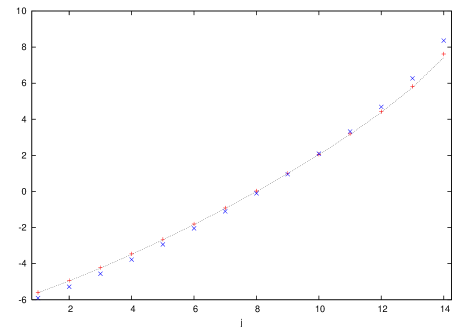
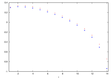
Figure 1: Check of (3.13) for a density $\rho\!=\!3x\sqrt{1\!-x^{2}}$ for which $x_{j}\!\!=\!\!\sqrt{1-(1\!-\!j/L)^{2/3}}$ with $j=1,..,L\!-\!1$ and $L=15$. $(a)$ The dotted line is the LHS of (3.13), while the $+$ are the RHS; the $\times$ denote the first term in the RHS. $(b)$ The $\ast$ represent the difference between the LHS and the first term in the RHS of (3.13), and the $+$ are the $1/L$ correction.

In the general situation on which the Bethe roots condense on several macroscopic curves, (3.13) will apply to the summation over roots belonging to each separate curve. When the roots $x_{j}$, $x_{k}$ lay on different curves, the last term on (3.13) is absent. Let us denote by $x_{s,j}$ the roots belonging to the $s$-th curve. The integral Bethe equations (2.5), valid in the limit of an infinite chain, gets modified as follows by the first finite size corrections

$${\epsilon\over x_{s,j}}\;+\;2\pi n_{s} = {1\over L}\,\sum_{k\neq j}{2\over x_{s,j}-x_{s,k}}\;+$$

$$+ {1\over L}\,\sum_{r\neq s}\sum_{k}{2\over x_{s,j}-x_{r,k}}\;+\;{\rho^{\prime}_{s,j}\over\rho_{s,j}L}\left(\pi\rho_{s,j}\coth\pi\rho_{s,j}-1\right)\;.$$

These equations can be straightforwardly generalized to spin chains based on general Lie groups.

We would like to end this section with a comment on the validity of (3.13) and (3). In deriving these equations, we have assumed that the number of roots around the chosen one $x_{s,j}$ is of order $L$. This stops being true for $x_{s,j}$ sufficiently close to the end points of the associated condensation curve. We expect that this problem does not affect the $1/L$ corrections to the conserved charges of the macroscopic Bethe solutions. However it will be important to estimate the order of the next to leading finite size effects. Let us look again to figure 1. In our example, the roots $x_{j}$ lay on the interval $[0,1]$. For $x$ close to $1$ the density is $\;\sim\!\sqrt{1-x}$, reproducing the typical behaviour of the densities which solve the Bethe equations. In figure 1b we observe that the $1/L$ correction that we have obtained is a worse approximation for $x$ close to $1$. In spite of that, this problem is practically confined to the last root.

It has been argued that quantum corrections to the conserved charges of spinning strings on $AdS_{5}\times S^{5}$ are suppressed by integer powers of $1/L$ [40, 53]. According to the AdS/CFT correspondence, quantum corrections to semiclassical strings map to finite size effects for the spin chain describing the spectrum of anomalous dimensions of ${\cal N}=4$ Yang-Mills. Hence it is interesting that, in addition to evaluating the leading finite size corrections for roots not very close to the end points, we were able to show that for them the next to leading effects are of order $1/L^{2}$.

4 Finite size corrections to the energy

We will now use the results of the previous section to calculate the leading finite size corrections to the energy of certain solutions to the Bethe equations for $SU(2)$ and $SU(1,1)$ spin chains. The energy is in both cases given by

$$E={\lambda\over 8\pi^{2}}\sum_{j=1}^{M}{1\over u_{j}^{2}+1/4}\approx{\lambda\over 8\pi^{2}L^{2}}\sum_{j=1}^{M}{1\over x_{j}^{2}}\;.$$ (4.1)

We will concentrate again in solutions of the Bethe equation where the roots condense on a single curve $\cal C$. The AdS/CFT correspondence relates these solutions to the simplest and most studied example of semiclassical strings spinning on $AdS_{5}\times S^{5}$, i.e. circular strings [5, 40, 41, 42]. The $SU(2)$ and $SU(1,1)$ cases correspond respectively to strings rotating with two angular momenta on $S^{5}$, or both on $S^{5}$ and $AdS_{5}$. Comparing the energies on both sides of the correspondence it will be possible to determine if the perfect agreement found in the thermodynamic/classical limit [27]-[31], extends to the finite size/quantum level.

The Bethe equations (3) reduce in the case of a single curve to

$${\epsilon\over x_{j}}\,+\,2\pi n\;=\;{1\over L}\,\sum_{k\neq j}{2\over x_{j}-x_{k}}\;+\;{\rho^{\prime}_{j}\over\rho_{j}L}\left(\pi\rho_{j}\coth\pi\rho_{j}-1\right)\;,$$ (4.2)

where $\epsilon=1,-1$ for the $SU(2)$ and $SU(1,1)$ cases, respectively. Defining $\alpha\!=\!{M\over L}$, the function $\rho(x)$ is given by [27, 28, 54]

$$\rho(x)\,=\,{\sqrt{8\pi n\alpha x-(2\pi nx+\epsilon)^{2}}\over 2\pi x}\;.$$ (4.3)

Summing (4.2) over $j$ we obtain

$$\sum_{j=1}^{M}{\epsilon\over x_{j}}\,=\,-2\pi nM\;+\int_{\Gamma}d\rho\left(\pi\rho\coth\pi\rho-1\right)\;,$$ (4.4)

where $\Gamma$ is the contour on the $\rho$-plane defined by the function $\rho(x)$, with $x\!\in\!{\cal C}$. Since on the end points of $\cal C$ the density is zero, the contour $\Gamma$ is closed and always contains the origin. For $SU(1,1)$ the curve $\cal C$ lies on the real axis and $\rho(x)$ is a real function. $\Gamma$ should be understood then as a closed contour surrounding the interval between the origin and the maximal value of the density, $\rho_{M}$ (see figure 2a). Hence the integral on (4.4) clearly vanishes. For $SU(2)$ the contour $\Gamma$ is symmetric under reflexion along the imaginary axes, to which it cuts at zero and the maximal value of the density, $|\rho_{M}|$ (see figure 2b). Depending on the values of $n$ and $\alpha$ this contour can encircle some of the poles of the integrand in (4.4), which lie at $\rho=i\mathbb{Z}^{\ast}$, implying that the integral does not vanish. We will not enter here the study of this more involved situation and its analysis in the context of the AdS/CFT correspondence. In this section we will consider only $SU(2)$ solutions for which $|\rho_{M}|\!<\!1$ and thus the integral on (4.4), as for the $SU(1,1)$ case, vanishes.

Figure 2: Contour $\Gamma$ for a) $SU(1,1)$ and b) $SU(2)$ cases. The dots, $\bullet$, are the points $\rho=0,\rho_{M}$. The crosses, $\times$, in figure b) represent the poles of $\pi\rho\coth\pi\rho$.

Multiplying (4.2) by $\epsilon/x_{j}$ and then summing we get

$$\sum_{j=1}^{M}{1\over x_{j}^{2}}\,=\,4\pi^{2}n^{2}M\;+\;{\epsilon\over L}\,\sum_{k\neq j}{2\over x_{j}(x_{j}-x_{k})}\;+\;\epsilon\int_{\Gamma}{d\rho\over x(\rho)}\big{(}\pi\rho\coth\pi\rho-1\big{)}\;.$$ (4.5)

The function $x(\rho)$ is obtained inverting (4.3)

$$x\,=\,{(2\alpha-\epsilon)\,n-\sqrt{4\,n^{2}\alpha(\alpha\!-\!\epsilon)-\rho^{2}}\over 2\pi(\rho^{2}+n^{2})}\;.$$ (4.6)

This is a double valued function with branch points at $\pm\rho_{\ast}$, with $\rho_{\ast}=2n\sqrt{\alpha(\alpha-\epsilon)}$. Since the condensation curve lies on the real axis for the $SU(1,1)$ case, it is clear that the maximal value of the density is attained at the branch point, $\rho_{M}=\rho_{\ast}$. The situation is rather different for $SU(2)$. The curve $\cal C$ forms an arc on the $x$-plane symmetric under reflexion along the real axis, whose precise location is determined by the condition that $\rho(x)dx$ should be real. This translates into a transcendental equation that can be analyzed numerically [46]. The maximal value of the density is attained at the intersection point between $\cal C$ and the real axis, and it turns out to verify $|\rho_{M}|>|\rho_{\ast}|$. The difference between $\rho_{M}$ and $\rho_{\ast}$ is maximal for the case of half-filling while for small $\alpha$, $\rho_{M}\rightarrow\rho_{\ast}$.

The spin chain dynamics can be alternatively described in the language of coherent states. The coherent states which correspond to the $SU(2)$ single curve solutions have been shown to be unstable when $|\rho_{\ast}|>1$ [34]. This condition does have a translation in terms of the Bethe solutions: some poles of the integrand in (4.4) lie between the branch points of the function $x(\rho)$. The fact that there are two different distinguished values of the density, $\rho_{M}$ and $\rho_{\ast}$, deserves a better understanding. It is important to stress that all $SU(2)$ solutions that can be mapped to ${\cal N}=4$ Yang-Mills operators, or equivalently, to semiclassical strings on $AdS_{5}\times S^{5}$ are unstable and thus have $|\rho_{M}|>1$. Hence they are excluded from the analysis below, which is restricted for the $SU(2)$ case to $|\rho_{M}|<1$.

The second term on the RHS of 4.5 is easily evaluated to be

$$\sum_{k\neq j}{2\over x_{j}(x_{j}-x_{k})}=-(2\pi nM)^{2}+\sum_{j=1}^{M}{1\over x_{j}^{2}}\,.$$ (4.7)

Using (4.1) we obtain for the leading contribution to the energy

$$E_{0}={\lambda\over 2L}n^{2}\alpha(1-\epsilon\alpha)\;,$$ (4.8)

which reproduces the results of [27, 28]. It is equivalent but more transparent to write the integral in (4.5) in terms of a contour ${\bar{\Gamma}}$ surrounding the branch cut of the function $x(\rho)$, lying between $\,\pm 2n\sqrt{\alpha(\alpha-\epsilon)}$. Then the leading finite size correction to the energy is

$$E_{1}={\epsilon\lambda\over 2L^{2}}\left[n^{2}\alpha(1-\epsilon\alpha)\;+\;{1\over 8\pi^{2}}\int_{\bar{\Gamma}}{d\rho\over x(\rho)}\big{(}\pi\rho\coth\pi\rho-1\big{)}\,\right]\;.$$ (4.9)

The first term comes from the $n\!=\!0$ piece in the approximation of the logarithm by a series expansion. It gives the contribution to the finite size effects calculated in [39, 28]. Contrary to the $SU(2)$ circular strings, the $SU(1,1)$ ones are stable. In [42] the leading quantum correction to their classical energy was calculated, finding that the first term in (4.9) only takes care of the zero mode fluctuations. A. Tseytlin has informed us that the last term in (4.9) restores the perfect agreement with the string results. This represents one of the strongest tests of the AdS/CFT correspondence obtained up to now.

It is interesting to compare expression (4.9) with the finite size corrections to the ground state energy $E(L)$ of a critical Hamiltonian $H$ defined in a strip of width $L$, which is given by $E_{0}(L)=-\pi c/(6L)$ where $c$ is the Virasoro central charge [55]. A well known example is the antiferromagnetic Heisenberg Hamiltonian, where $c=1$, which is at the heart of the bosonization approach to this spin chain [56]. In a relativistic $1+1$ model, where $E\sim k$, one can exchange time and space. Therefore the previous formula can also be seen as the free energy per unit length $F/(k_{B}T)$, which yields a low temperature specific heat $C\sim\pi ck_{B}^{2}T/3$. In the case of equation (4.9) the $1/L$ correction does not have such a CFT interpretation, since for the dual string it simply corresponds to the classical energy. However, the quantum corrections of the string, given by the zero point energy, appear in the next order correction, ${\cal O}(L^{-2})$, to the energy and in that sense are the analogue of the $c$ term. This is related to the fact that a ferromagnetic system has a dispersion relation $E\sim k^{2}$, so that time, which is an inverse temperature, should be exchanged by (space)². Hence we expect a correspondence between the finite size effects for the ferromagnetic Hamiltonian and the finite temperature effects of the system in infinite size, where all the low energy excitations contribute.

5 Conclusions

In this paper we have considered finite size corrections to the thermodynamic limit of the Bethe ansatz for the $SU(2)$ and $SU(1,1)$ ferromagnetic spin chains. Anomalous dimensions of large ${\cal N}=4$ Yang-Mills operators can be computed by solving the Bethe ansatz for the corresponding spin chain, and compared with the energies of strings with two angular momenta rotating entirely along $S^{5}$ in the $SU(2)$ case, or both along $AdS_{5}$ and $S^{5}$ in the $SU(1,1)$ sector. Therefore our computation of the finite length effects provides the leading order correction, in $1/L$, to the anomalous dimensions of the operators. The finite size effects correspond, on the dual string theory side, to quantum corrections to classical string solutions. Hence the first $1/L$ correction that we have found represents, following the AdS/CFT correspondence, the one-loop correction to the string energy.

The finite size Bethe ansatz equations that we have obtained, including the $1/L$ correction, may allow for a comparison with the string dynamics along the lines of [27, 28, 29]. This would imply not only the matching with the energy, but also with the complete tower of conserved charges. The extension of the perfect agreement between the integrable structure associated to long Yang-Mills operators and that of classical strings on $AdS_{5}\times S^{5}$ to the first quantum corrections would be a most remarkable test of the AdS/CFT correspondence.

Acknowledgments

It is a pleasure to thank A. Tseytlin for numerous discussions and informing us of their work prior to publication [57]. We are also grateful to C. Gómez and K. Zarembo for comments and correspondence. E. L. was supported by a Ramón y Cajal contract of the MCYT and in part by the Spanish DGI under contract FPA2003-04597. A. P. was supported by a Spanish fellowship FPI. Finally G. S. has been supported by Spanish DGES under contract BFM2003-05316-C02-01. We also thank the EC Commission for financial support via the FP5 Grant HPRN-CT-2002-00325.

References

- [1]
- [2] A. M. Polyakov, Gauge fields and space-time, Int. J. Mod. Phys. A 17S1 (2002) 119, hep-th/0110196.
- [3] D. Berenstein, J. M. Maldacena and H. Nastase, Strings in flat space and pp waves from N = 4 super Yang Mills, JHEP 0204 (2002) 013, hep-th/0202021.
- [4] S. S. Gubser, I. R. Klebanov and A. M. Polyakov, A semi-classical limit of the gauge/string correspondence, Nucl. Phys. B 636 (2002) 99, hep-th/0204051.
- [5] S. Frolov and A. A. Tseytlin, Multi-spin string solutions in , Nucl. Phys. B 668 (2003) 77, hep-th/0304255. S. Frolov and A. A. Tseytlin, Rotating string solutions: AdS/CFT duality in non-supersymmetric sectors, Phys. Lett. B 570 (2003) 96, hep-th/0306143. G. Arutyunov, S. Frolov, J. Russo and A. A. Tseytlin, Spinning strings in : New integrable system relations, Nucl. Phys. B 671 (2003) 3, hep-th/0307191. G. Arutyunov, J. Russo and A. A. Tseytlin, Spinning strings in and integrable systems, Nucl. Phys. B 671 (2003) 3, hep-th/0311004.
- [6] N. Beisert, C. Kristjansen and M. Staudacher, The dilatation operator of super Yang-Mills theory, Nucl. Phys. B 664 (2003) 131, hep-th/0303060.
- [7] N. Beisert, The complete one-loop dilatation operator of super Yang-Mills theory, Nucl. Phys. B 676 (2004) 3, hep-th/0307015.
- [8] J. A. Minahan and K. Zarembo, The Bethe-ansatz for super Yang-Mills, JHEP 0303 (2003) 013, hep-th/0212208.
- [9] N. Beisert and M. Staudacher, The SYM integrable super spin chain, Nucl. Phys. B 670 (2003) 439, hep-th/0307042.
- [10] N. Beisert, J. A. Minahan, M. Staudacher and K. Zarembo, Stringing spins and spinning strings, JHEP 0309 (2003) 010, hep-th/0306139.
- [11] N. Beisert, S. Frolov, M. Staudacher and A. A. Tseytlin, Precision spectroscopy of AdS/CFT, JHEP 0310 (2003) 037, hep-th/0308117.
- [12] G. Arutyunov and M. Staudacher, Matching higher conserved charges for strings and spins, JHEP 0403 (2004) 004, hep-th/0310182.
- [13] J. Engquist, J. A. Minahan and K. Zarembo, Yang-Mills duals for semiclassical strings on , JHEP 0311 (2003) 063, hep-th/0310188.
- [14] D. Serban and M. Staudacher, Planar gauge theory and the Inozemtsev long range spin chain, JHEP 0406 (2004) 001, hep-th/0401057.
- [15] C. Kristjansen, Three-spin strings on from SYM, Phys. Lett. B 586 (2004) 106, hep-th/0402033.
- [16] J. Engquist, Higher conserved charges and integrability for spinning strings in , JHEP 0404 (2004) 002, hep-th/0402092.
- [17] G. Arutyunov and M. Staudacher, Two-loop commuting charges and the string / gauge duality, hep-th/0403077.
- [18] H. Dimov and R. C. Rashkov, A note on spin chain / string duality, hep-th/0403121. H. Dimov and R. C. Rashkov, Generalized pulsating strings, JHEP 0405 (2004) 068, hep-th/0404012.
- [19] G. Ferretti, R. Heise and K. Zarembo, New integrable structures in large-N QCD, Phys. Rev. D 70 (2004) 074024, hep-th/0404187.
- [20] N. Beisert, V. Dippel and M. Staudacher, A novel long range spin chain and planar super Yang-Mills, JHEP 0407 (2004) 075, hep-th/0405001.
- [21] M. Smedbäck, Pulsating strings on , JHEP 0407 (2004) 004, hep-th/0405102.
- [22] L. Freyhult, Bethe ansatz and fluctuations in Yang-Mills operators, JHEP 0406 (2004) 010, hep-th/0405167.
- [23] J. A. Minahan, Higher loops beyond the sector, JHEP 0410, 053 (2004), hep-th/0405243.
- [24] C. Kristjansen and T. Mansson, The circular, elliptic three-spin string from the SU(3) spin chain, Phys. Lett. B 596 (2004) 265, hep-th/0406176.
- [25] G. Arutyunov, S. Frolov and M. Staudacher, Bethe ansatz for quantum strings, JHEP 0410 (2004) 016, hep-th/0406256.
- [26] S. Ryang, Circular and folded multi-spin strings in spin chain sigma models, JHEP 0410 (2004) 059, hep-th/0409217.
- [27] V. A. Kazakov, A. Marshakov, J. A. Minahan and K. Zarembo, Classical / quantum integrability in AdS/CFT, JHEP 0405 (2004) 024, hep-th/0402207.
- [28] V. A. Kazakov and K. Zarembo, Classical / quantum integrability in non-compact sector of AdS/CFT, JHEP 0410 (2004) 060, hep-th/0410105.
- [29] N. Beisert, V. A. Kazakov and K. Sakai, Algebraic curve for the SO(6) sector of AdS/CFT, hep-th/0410253.
- [30] G. Arutyunov and S. Frolov, Integrable Hamiltonian for classical strings on , JHEP 0502 (2005) 059, hep-th/0411089.
- [31] S. Schafer-Nameki, The algebraic curve of 1-loop planar SYM, hep-th/0412254.
- [32] M. Kruczenski, Spin chains and string theory, Phys. Rev. Lett. 93 (2004) 161602, hep-th/0311203.
- [33] M. Kruczenski, A. V. Ryzhov and A. A. Tseytlin, Large spin limit of string theory and low energy expansion of ferromagnetic spin chains, Nucl. Phys. B 692 (2004) 3, hep-th/0403120.
- [34] R. Hernández and E. López, The spin chain sigma model and string theory, JHEP 0404 (2004) 052, hep-th/0403139.
- [35] B. J. Stefanski and A. A. Tseytlin, Large spin limits of AdS/CFT and generalized Landau-Lifshitz equations, JHEP 0405 (2004) 042, hep-th/0404133.
- [36] M. Kruczenski and A. A. Tseytlin, Semiclassical relativistic strings in and long coherent operators in SYM theory, JHEP 0409 (2004) 038, hep-th/0406189.
- [37] S. Bellucci, P. Y. Casteill, J. F. Morales and C. Sochichiu, spin chain and spinning strings on , Nucl. Phys. B 707 (2005) 303, hep-th/0409086.
- [38] R. Hernández and E. López, Spin chain sigma models with fermions, JHEP 0411 (2004) 079, hep-th/0410022.
- [39] M. Lubcke and K. Zarembo, Finite-size corrections to anomalous dimensions in N = 4 SYM theory, JHEP 0405 (2004) 049, hep-th/0405055.
- [40] S. Frolov and A. A. Tseytlin, Quantizing three-spin string solution in , JHEP 0307 (2003) 016, hep-th/0306130.
- [41] S. A. Frolov, I. Y. Park and A. A. Tseytlin, On one-loop correction to energy of spinning strings in , Phys. Rev. D 71 (2005) 026006, hep-th/0408187.
- [42] I. Y. Park, A. Tirziu and A. A. Tseytlin, Spinning strings in : One-loop correction to energy in sector, hep-th/0501203.
- [43] L. Freyhult and C. Kristjansen, Finite Size Corrections to Three-spin String Duals, hep-th/0502122.
- [44] R. W. Richardson, Pairing in the limit of a large number of particles, J. Math. Phys. 18 (1977) 1802.
- [45] M. Gaudin, “États propres et valeurs propres de l’Hamiltonien d’appariement”, unpublished Saclay preprint, 1968. Included in Travaux de Michel Gaudin, Modèles exactament résolus, Les Éditionsde Physique, France, 1995.
- [46] J. M. Román, G. Sierra and J. Dukelsky, Large N limit of the exactly solvable BCS model: analytics versus numerics, Nucl. Phys. B 634 (2002) 483, cond-mat/0202070.
- [47] J. Dukelsky, S. Pittel and G. Sierra, Exactly solvable Richardson-Gaudin models for many-body quantum systems, Rev. Mod. Phys. 76 (2004) 643-662, nucl-th/0405011.
- [48] R.W. Richardson and N. Sherman, Exact eigenstates of the pairing-force Hamiltonian, Nucl. Phys. B 52 (1964) 221.
- [49] R.W. Richardson, Exactly Solvable Many-Boson Model, J. Math. Phys. 9 1327 (1968).
- [50] J. Dukelsky and P. Schuck, Condensate Fragmentation in a New Exactly Solvable Model for Confined Bosons, Phys. Rev. Lett. 86 (2001) 4207, cond-mat/0009057.
- [51] A. LeClair, J. M. Román and G. Sierra, Russian Doll Renormalization Group and Superconductivity, Phys. Rev. B 69 (2004) 20505, cond-mat/0211338.
- [52] A. Anfossi, A. LeClair and G. Sierra, The elementary excitations of the exactly solvable russian doll BCS model of superconductivity, to appear.
- [53] A. A. Tseytlin, Spinning strings and AdS/CFT duality, hep-th/0311139.
- [54] A. A. Ovchinnikov, On the exactly solvable pairing models for bosons, JSTAT 0407 (2004) P004, math-ph/0405047.
- [55] J. Cardy, “Scaling and Renormalization in Statistical Physics”, Cambridge University Press, U.K. (1997).
- [56] A. O. Gogolin, A.A. Nersesyan and A.M. Tsvelik, “Bosonization and Strongly Correlated Systems”, Cambridge University Press, U.K. (1998).
- [57] N. Beisert, A. A. Tseytlin and K. Zarembo, Matching quantum strings to quantum spins: one-loop vs. finite size corrections, ITEP-TH-12/05, PUTP-2151, UUITP-02/05, hep-th/0502173.