Cosmological constraints on string scale and coupling arising from tachyonic instability

Abstract:

We demonstrate that string motivated inflation ending via tachyonic instability leaves a detectable imprint on the cosmic microwave background (CMB) radiation by virtue of the excitation of non-Gaussian gravitational fluctuations. The present WMAP bound on non-Gaussianity is shown to constrain the string scale by $M_{S}/M_{P}\leq 10^{-4}$ for string coupling $g_{s}<0.1$, hence improving the existing bounds. If tachyon fluctuations during inflation are not negligible, we find the stringent constraint $g_{s}\sim 10^{-9}$ for $M_{S}/M_{P}<10^{-3}$. This case may soon be ruled out by the forthcoming CMB non-Gaussinianity bounds.

1 Introduction and Summary

Currently the main hope for detecting signatures of string theory relies on the cosmic laboratory. In particular, the cosmic microwave background (CMB) signals of an early inflationary phase, which could have a stringy origin. One possibility discussed in the literature is a period of accelerated expansion induced by the dynamics of two parallel branes [1, 2, 3, 4]. A D-brane $Dp$ and an anti-D-brane $\widetilde{Dp}$ approach each other, giving rise to inflation, which ends when the branes annihilate, or equivalently by virtue of a tachyonic instability that arises when the branes approach each other to within the string length [2, 3, 4]. Here the tachyon is a collective description of excited open string degrees of freedom representing the breaking of space time supersymmetry and the resulting vacuum instability. Tachyons are also found in bosonic string theory and in the context of a non-BPS brane configurations [5], suggesting that their appearance is quite common in string theory.

The process of $Dp$-$\widetilde{Dp}$ annihilation and the associated tachyon dynamics can be depicted in terms of an effective scalar field theory with a negative mass squared potential [6]. However, it has turned out to be extremely difficult to get enough e-foldings of inflation in string motivated inflationary models in general. Both well studied $Dp$-$\widetilde{Dp}$ inflation [7] and the race track models [8] have a difficulty in generating a large enough number of e-foldings, about $N\sim 65$. If inflation occurs in a number of subsequent bouts, it is however possible to relax [9] the bound on $N$, and the minimum number of e-foldings could be as low as $12$ in order to explain the large scale structure and the CMB data; another $20$ to $30$ e-foldings are needed to solve the flatness problem. However, here we do not commit ourselves to one particular view but rather simply assume that enough e-foldings will be obtained and that eventually inflation ends via a tachyonic instability. As we will show, then there exists a direct test of string cosmology: the tachyonic instability gives rise to non-Gaussianity in the primordial perturbations (for a review of non-Gaussianity, see [10]). Moreover, such non-Gaussian features can easily be observable and, by virtue of the WMAP data [15], are already constrained.

In the string theory setup, the tachyon field rolls down from the top of the potential after the end of inflation. As the field rolls down quickly through the region where the effective mass squared is still negative, the first order matter perturbations grow exponentially similarly to the case of well-studied tachyonic preheating [11] . Following our previous analysis, [13], one then finds that the growth in the matter perturbations seed the second order metric fluctuations and gives rise to large non-Gaussianity in the CMB temperature fluctuation spectrum. As will be discussed below, the present observable limits [15] on non-Gaussianity can then be used to constraint the string scale, $M_{S}$, and the string coupling, $g_{s}$.

We consider two particular scenarios. In both the cases the initial fluctuations of the tachyon matter is created during inflation. However in order to keep our analysis as general as possible, we consider the first case where the first order metric perturbations, $\phi^{(1)}={\rm constant}$, has a trivial solution, which is dominated by the amplitude of the existing perturbations during inflation. In this case we obtain a bound on the string scale: $M_{S}/M_{P}\leq 10^{-4}$ for $g_{s}\leq 0.1$. In the second scenario we assume the growing solution for $\phi^{(1)}$, in which case we obtain a stringent constraint on the string coupling, given by $g_{s}\sim 10^{-9}$ for $M_{S}/M_{P}\sim 10^{-3}$. Future observational limits on non-Gaussianity can soon render the latter scenario incompatible with the observed CMB temperature fluctuation amplitude of $10^{-5}$.

2 Gravitational perturbations and the tachyon

For simplicity we focus on the bosonic action for the tachyon. The discussion can be easily generalized to the superstring case. The 4D effective field theory action of the tachyon field $T$ on a D3-brane, computed in a bosonic string theory around the top of the potential, reads as (up to higher derivative terms) [16, 17]

$$S_{B}=-\tau_{3}\int d^{4}x\sqrt{-g}\left(\alpha^{\prime}e^{-T}\partial_{\mu}T\partial^{\mu}T+(1+T)e^{-T}\right)\,,$$ (1)

where the brane tension is given by

$$\tau_{3}=\frac{M_{S}^{4}\sqrt{2}}{(2\pi)^{3}g_{s}}.$$ (2)

Here $g_{s}$ is the string coupling and $M_{S}=1/l_{s}=1/\sqrt{\alpha^{\prime}}$ are the fundamental string mass and length scales.

The form of the tachyon action given in Eq. (1) is not immediately suitable for the purposes of perturbation equations at second order. It is convenient first to transform the action into a canonical form by the redefinition

$$T=-2\,\textrm{ln}\left(\frac{\varphi}{2\sqrt{2\tau_{3}\alpha^{\prime}}}\right).$$ (3)

The potential for the redefined tachyon $\varphi$ reads as

$$V(\varphi)=\frac{1}{8}\,M_{S}^{2}\varphi^{2}\left[1-2\,\textrm{ln}\left(\frac{\varphi}{\varphi_{\max}}\right)\right],$$ (4)

where the definitions of $\tau_{3}$ and $\alpha^{\prime}$ have been used and

$$\varphi_{\max}\equiv 2\sqrt{2\tau_{3}\alpha^{\prime}}=M_{S}\sqrt{\frac{\sqrt{2}}{\pi^{3}\,g_{s}}}\,.$$ (5)

The transition $T=0\rightarrow\infty$ corresponds to $\varphi$ evolving from the maximum of the potential at $\varphi_{\max}$ to $\varphi=0$. The tachyonic instability is present when $V^{\prime\prime}(\varphi)<0$ or $1/\textrm{e}<\varphi/\varphi_{\max}\leq 1$. Because of the instability, the occupation number of $\varphi$ quanta grows exponentially.

In the simplest brane anti-brane inflationary scenarios the inflaton is the modulus $\sigma$, which is governed by the brane anti-brane separation or the angular separation between the two branes. In either case the inflaton potential can be separated from the tachyon potential, such that the total potential is given by [2, 3],

$$V=V(\sigma)+V(\varphi)\,.$$ (6)

The potential of $V(\sigma)$ depends on twice the brane tensions $2\tau_{3}$ and $\sigma$. In this paper we do not have to know the exact form of $V(\sigma)$, which can be found in Refs. [2, 3]. However for the purpose of simplifying our analysis we demand that after the end of inflation, when the tachyon starts rolling, the VEV of the inflaton is vanishing, $\langle\sigma\rangle=0$. This can be achieved by proper redefinition of the modulus around the string scale $M_{S}$.

The tachyon field and the inflaton field can be divided into the background and the first and the second order perturbation after inflation:

$$\varphi = \varphi_{0}(\eta)+\delta^{(1)}\varphi(\eta,{\bf x})+\frac{1}{2}\delta^{(2)}\varphi(\eta,{\bf x})\,.$$ (7)

$$\sigma = \delta^{(1)}\sigma(\eta,{\bf x})+\frac{1}{2}\delta^{(2)}\sigma(\eta,{\bf x})\,.$$ (8)

Here $\eta$ denotes the conformal time. The field perturbation gives rise to the metric perturbation (for details see Ref. [10] and references therein), which up to the second order reads $\phi=\phi^{(1)}+\phi^{(2)}/2$ with [18]

$$g_{00} = -a(\eta)^{2}\left(1+2\phi^{(1)}+\phi^{(2)}\right)\,,$$ (9)

$$g_{0i} = 0\,,$$ (10)

$$g_{ij} = a(\eta)^{2}\left(1-2\psi^{(1)}-\psi^{(2)}\right)\delta_{ij}\,,$$ (11)

where the generalized longitudinal gauge is used and the vector and tensor perturbations are neglected. Here $a(\eta)$ is the scale factor. The background equations of motion are then found to be

$$3{\cal H}^{2} = \frac{1}{2M_{P}^{2}}\varphi_{0}^{\prime\,2}+\frac{a^{2}}{M_{P}^{2}}V(\varphi_{0})\,,$$ (12)

$$0 = \varphi_{0}^{\prime\prime}+2{\cal H}\varphi_{0}^{\prime}+a^{2}V^{\prime}(\varphi_{0})\,,$$ (13)

while the $\sigma_{b}$-equation is trivial. Here $\cal H$ denotes the Hubble expansion rate expressed in conformal time and the reduced Planck scale is given by $M_{P}=2.4\times 10^{18}$ GeV. The relevant first order perturbation equations can be written in the form [19, 14, 13]

$$\phi^{(1)\,^{\prime\prime}}-\partial_{i}\partial^{i}\phi^{(1)}+2\left({\cal H}-\frac{\varphi_{0}^{\prime\prime}}{\varphi_{0}^{\prime}}\right)\phi^{(1)\,^{\prime}}+2\left({\cal H}^{\prime}-\frac{\varphi_{0}^{\prime\prime}}{\varphi_{0}^{\prime}}{\cal H}\right)\phi^{(1)} = 0\,.$$ (14)

$$\delta^{(1)}\sigma^{\prime\prime}+2{\cal H}\delta^{(1)}\sigma^{\prime}-\partial_{i}\partial^{i}\delta^{(1)}\sigma+g^{2}\varphi_{0}^{2}\,\delta^{(1)}\sigma = 0\,.$$ (15)

All the information regarding $\delta^{(1)}\varphi$ is contained in Eq. (14), whose right hand side is zero by virtue of $\langle\sigma\rangle=0$, see [23]. Further note that there are no metric perturbations in Eq. (15). This is due to assuming a vanishing VEV for $\sigma$. Hence the $\sigma$ part can be solved separately.

At the second order we are only interested in the gravitational perturbation arising due to the tachyon and the inflaton field. The gravitational perturbation equation can be written in an expanding background as [19, 14, 13]

$${\phi^{(2)^{\prime\prime}}}+2\left({\cal H}-\frac{\varphi^{\prime\prime}_{0}}{\varphi^{\prime}_{0}}\right){\phi^{(2)^{\prime}}}+2\left({\cal H}^{\prime}-\frac{\varphi^{\prime\prime}_{0}}{\varphi^{\prime}_{0}}{\cal H}\right){\phi^{(2)}}-\partial_{i}\partial^{i}{\phi^{(2)}}=$$

$${\cal J}_{\varphi,\textrm{local}}+{\cal J}_{\sigma,\textrm{local}}+{\cal J}_{\textrm{non-local}}$$ (16)

where the source terms $\cal J$ are quadratic combinations of first order perturbations; in particular [19, 18],

$${\cal J}_{\varphi,\textrm{local}} = -\frac{1}{M_{P}^{2}}\left[2(\delta^{(1)}\varphi^{\prime})^{2}+8(\varphi_{0}^{\prime})^{2}(\phi^{(1)})^{2}-a^{2}V_{,\varphi\varphi}(\delta^{(1)}\varphi)^{2}-8\varphi_{0}^{\prime}\phi^{(1)}\delta^{(1)}\varphi^{\prime}\right]$$ (17)

$$-24{\cal H}^{\prime}(\phi^{(1)})^{2}-24{\cal H}\phi^{(1)}\phi^{(1)\,^{\prime}}$$

$${\cal J}_{\sigma,\textrm{local}} = -\frac{2}{M_{P}^{2}}(\delta^{(1)}\sigma^{\prime})^{2}+\frac{a^{2}}{M_{P}^{2}}\frac{\partial^{2}V}{\partial\sigma^{2}}(\delta^{(1)}\sigma)^{2}~{}\,,$$ (18)

$${\cal J}_{\textrm{non-local}} = \triangle^{-1}f(\delta^{(1)}\varphi,\delta^{(1)}\sigma,\phi^{(1)})\,,$$ (19)

where $f$ is a quadratic function of the first order fluctuations and the coefficients depend on background quantities. Because of the inverse Laplacian the last source term is non-local. Typically such term contains: $\triangle^{-1}(\phi^{(1)\,^{\prime}}\triangle\phi^{(1)})$, $\triangle^{-1}(\partial_{i}\delta^{(1)}\varphi\partial^{i}\delta^{(1)}\varphi),\ldots$ Note that the left hand side of Eq. (16) is identical to the first order equation, see Eq. (14). $\cal J_{\textrm{non-local}}$ involves an inverse spatial Laplacian, thus rendering it non-local .

3 Estimating non-Gaussianity

Let us assume that the unstable modes grow within a time interval much smaller than the Hubble rate in Eq. (14). This means that the tachyon field evolves fast enough so that we can neglect the effects of the expansion. Then conformal time and cosmic time are equal with $\eta=t$ and $a=1$ and in the large wavelength limit we then obtain

$$\ddot{\phi}^{(1)}-2A\,\dot{\phi}^{(1)}=0\,,$$ (20)

where $A=\ddot{\varphi}_{0}/\dot{\varphi}_{0}$. With the assumption that the tachyonic stage is so short so that $\dot{\varphi}_{0},\,\ddot{\varphi}_{0}$ are effectively constants, there will be two solutions: a constant $\phi^{(1)}$; and an exponentially growing solution $\phi^{(1)}\propto\exp(2At)$. The amplitudes of the two solutions are determined by the initial conditions.

In the brane-anti-brane case, the dynamics of $\varphi$ is decoupled from inflation; therefore no instability occurs during the initial phase of inflation. During which the tachyon fluctuations is also suppressed and negligible. However as the branes move close to each other the tachyonic instability is triggered. Let us assume that the scale of inflation is such that $H_{inf}\sim M_{S}$ during the last ${\cal O}(5-10)$ e-foldings of inflation, then the tachyon feels the vacuum induced long wavelength fluctuations during inflation. Note that these fluctuations are isocurvature in nature. Let us first investigate the scenario where $\phi^{(1)}={\rm constant}$. This assumes that no amplification in $\phi^{(1)}$ has taken place due to the rolling tachyon. By virtue of the observed temperature anisotropies we take $\phi^{(1)}\sim 10^{-5}$, as we shall see that this conclusion does not hold for higher order metric perturbations. They will be amplified in order to give rise to a significant non-Gaussianity.

When the brane separation becomes of the order of string length, the mass squared of $\varphi$ field becomes negative. We assume this happens when the inflaton $\sigma\rightarrow 0$. During this epoch the fluctuations of the tachyon field grow exponentially for all the momenta $k<M_{S}/\sqrt{2}$. The dispersion of the growing modes at $t>0$ is given by [11]

$$\langle\delta\varphi^{2}\rangle=\int_{0}^{M_{S}/\sqrt{2}}\frac{dk^{2}}{8\pi^{2}}e^{2t\sqrt{M_{S}^{2}/2-k^{2}}}=\frac{e^{\sqrt{2}M_{S}t}(\sqrt{2}M_{S}t-1)+1}{16\pi^{2}t^{2}}\,.$$ (21)

The growth of the fluctuations continues until the fluctuations can modify the background equations of motion. This happens when Eq. (21) reaches $\langle\delta\varphi\rangle\sim\sqrt{\varphi_{max}/e}$, or until the time span $t_{\ast}\sim(\sqrt{2}/M_{S})\ln(4\pi\varphi_{max}/M_{S})$. During this period the number density of the tachyon quanta is then given by [11]

$$n_{k}\sim e^{\sqrt{2}M_{S}t_{\ast}}\sim\frac{16\sqrt{2}}{\pi g_{s}}\,.$$ (22)

In the limit when $g_{s}$ becomes vanishingly small the number density of excited tachyonic quanta diverges. This phenomena is easy to understand. In the small coupling limit the brane tension becomes large. Therefore a large potential energy density becomes available to the excited quanta. A similar situation is found in the tachyonic preheating case [11, 13].

The total energy density stored in the produced $\varphi$ quanta is given by

$$\rho_{\varphi}\sim\frac{1}{2}(\delta^{(1)}\dot{\varphi})^{2}\sim\frac{M_{S}^{4}}{3B^{3}g_{s}}\,.$$ (23)

where $B=\pi/\sqrt{2}$. The equation for the second order metric perturbation now includes a source term which includes perturbations from the inflaton, ${\cal J}_{\sigma,\textrm{local}}$ and ${\cal J}_{\varphi,\textrm{local}}$. However when the tachyon is rolling the inflaton fluctuations are negligible compared to that of the tachyon. This allows us to keep only the tachyonic source terms, which in the long wavelength regime reads as

$$\ddot{\phi}^{(2)}\sim-\frac{4M_{S}^{4}}{3B^{3}g_{s}M_{P}^{2}}\,.$$ (24)

Integrating the above equation over the time interval $t_{\ast}\sim(\sqrt{2}/M_{S})\ln(4\pi\varphi_{max}/M_{S})$, we find $\phi^{(2)}\sim-(4/3B^{3}g_{s})(M_{S}/M_{P})^{2}\ln^{2}(4/\sqrt{Bg_{s}})$. An important point to note here is that the second order metric perturbations, $\phi^{(2)}$, are mainly sourced by the tachyon matter fluctuations.

The non-Gaussianity parameter during the rolling of the tachyon, when the first order metric perturbation stays constant, is then roughly given by

$$f_{NL}^{\phi}\sim\frac{\phi^{(2)}}{(\phi^{(1)})^{2}}\sim-\frac{4\cdot 10^{10}}{3B^{3}g_{s}}\left(\frac{M_{S}}{M_{P}}\right)^{2}\ln^{2}\left(\frac{4}{\sqrt{Bg_{s}}}\right)\,.$$ (25)

The parameter $f_{NL}^{\phi}$ is related to the standard non-Gaussianity parameter $f_{NL}$ by $f_{NL}=-f_{NL}^{\phi}+11/6$ [10]. The present bound from WMAP is given by the range $-132<f_{NL}^{\phi}<60$ $@~{}95\%$ [15], In Fig. 1 we have plotted the $f_{NL}^{\phi}=-132$ curve based on Eq. (25). The allowed parameter space is below the curve.

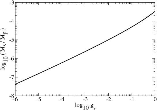
Figure 1: Allowed region is below the curve, which gives $f_{NL}^{\phi}=-132$.

It has been argued that an unavoidable consequence of brane inflation is a network of cosmic strings that appears at the end of inflation [20]. If true, and assuming that the amount of cosmic strings produced is the highest possible allowed by the current CMB data, which is less than $10\%$ of the total energy density, then the CMB and LSS data would imply a bound $G\mu<10^{-6}$ on the string tension $\mu$ [21] (here $G$ is the Newton’s constant). A search of cosmic strings in the WMAP 1-year data has been shown to lead to the limit $G\mu<10^{-6.5}$ [22]. For a fixed dilaton, these bounds translate to bounds on the string scale, given respectively by $M_{S}/M_{P}<10^{-3}$ and $M_{S}/M_{P}<10^{-3.25}$.

Limits from non-Gaussianity, as given by Fig. 1, yield an improved constraint on the string scale if we require that the string coupling $g_{s}<1$. For instance, if $g_{s}\sim 10^{-1}$, as is appropriate for the grand unified theories, we find a bound on the string scale given by $M_{S}/M_{P}\leq 10^{-4}$.

4 Consequences of tachyon fluctuations during inflation

Let us now consider the other extreme case, when the first order metric perturbation would be dominated by the exponentially growing solution so that $\phi^{(1)}\propto\exp(2At)$. This can happen when the initial fluctuations in $\varphi$ is large enough to overcome the constant solution for $\phi^{(1)}$. In this case the bound on the string scale and the string coupling will be more stringent than the one obtained in the previous Section, as we will now discuss.

Following Eq. (16) we may write

$$\ddot{\phi}^{(2)}-2A\,\dot{\phi}^{(2)}=-\frac{1}{M_{P}^{2}}\left[2(\delta^{(1)}\dot{\varphi})^{2}+8\dot{\varphi}_{0}^{2}(\phi^{(1)})^{2}-V_{,\varphi\varphi}(\delta^{(1)}\varphi)^{2}-8\dot{\varphi}_{0}\phi^{(1)}\delta^{(1)}\dot{\varphi}\right],$$ (26)

where we assumed that the right hand side is mainly sourced by the exponential instability triggered by the tachyon. Note that $\delta^{(1)}\varphi$ can be solved through the Einstein constraint [10]

$$\delta^{(1)}\varphi=\frac{2M_{P}^{2}}{\dot{\varphi}_{0}}\left(\dot{\phi}^{(1)}+H\phi^{(1)}\right)\,,$$ (27)

which is valid only if the backround value of the second scalar field vanishes $\sigma_{b}=0$. As discussed in [13], now $\phi^{(2)}$ contains a homogeneous solution $\sim\exp(2At)$ together with a source part $\sim\exp(4At)$. After a while the source part dominates and we obtain for the non-Gaussianity parameter,

$$f_{NL}^{\phi}=\frac{\phi^{(2)}}{(\phi^{(1)})^{2}}=8+\frac{M_{P}^{2}2V_{,\varphi\varphi}}{\dot{\varphi}_{0}^{2}}-\frac{4M_{P}^{2}\ddot{\varphi}_{0}^{2}}{\dot{\varphi}_{0}^{4}}-\frac{\dot{\varphi}_{0}^{4}}{M_{P}^{2}\ddot{\varphi}_{0}^{2}}\,.$$ (28)

Here we neglect a possible but small time variation in $A$.

The region of tachyonic growth occurs near $\varphi_{0}\approx\varphi_{\max}$ so that we obtain

$$f_{NL}^{\phi}\approx 8-16Cg_{s}\left(\frac{M_{P}}{M_{S}}\right)^{2}-\frac{1}{Cg_{s}}\left(\frac{M_{S}}{M_{P}}\right)^{2}-2Cg_{s}\left(\frac{M_{P}}{M_{S}}\right)^{2}\rm{ln}^{2}\left(\frac{4\pi}{(C~{}g_{s})^{1/2}}\right)\,,$$ (29)

where $C=\pi^{3}/\sqrt{2}$. It is easy to see that $f_{NL}^{\phi}$ is bounded from above by $f_{NL}^{\phi}\mathrel{\raise 1.29167pt\hbox{$<$\kern-8.50006pt\lower 4.30554pt\hbox{$\sim$}}}8$, which is comfortably within the current experimental bounds. On the other hand, there is no lower bound on $f_{NL}^{\phi}$, allowing us to set constraints on the values of $M_{S}/M_{P}$ and $g_{s}$. In Fig. 2 we show the allowed region (between the lines) for different values of $f_{NL}^{\phi}$. The current WMAP lower bound $-132<f_{NL}^{\phi}$ $@~{}95\%$ c.l. [15] corresponds to the contour given by the solid line in Fig. 2.

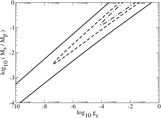
Figure 2: The contours given by the solid, dashed and dot-dashed lines correspond the non-linearity parameters $f_{NL}^{\phi}=-132,\,-20,\,-10$ respectively.

The non-Gaussianity constraint on the string coupling $g_{s}$ can be seen to be quite stringent. For $M_{S}/M_{P}\leq 10^{-3}$, from Fig. 2 one finds $g_{s}\sim 10^{-9}$. A future, improved bound on $f_{NL}^{\phi}$ would move the ratio $M_{S}/M_{P}$ towards one, rendering such models incompatible with the CMB observations because a too large anisotropy would be imparted onto the temperature fluctuations. Further note that the present considerations can be used to rule out low scale brane-anti-brane inflation, which would give rise to a large non-Gaussianity parameter.

In summary, if there is a large isocurvature component during inflation due to the fluctuations of the tachyon, then brane-anti-brane inflation ending via tachyon condensation is in great troubles. The present level of observational sensitivity to non-Gaussianity can already rule out a large part of the parameter space and requires a very small string coupling. In such a case the challenge for string cosmology would be to build brane-anti-brane inflationary models with $H\ll M_{S}$. For such a large $M_{S}$, the isocurvature perturbations of the tachyon will be very much suppressed during inflation, thereby evading our bounds depicted in Fig. 2. Otherwise when the isocurvature component is small then we can improve the obtained bound on the string scale $M_{S}/M_{P}\leq 10^{-4}$.

Note that our conclusions hold for a tachyonic instability occurring in bosonic strings, but a similar analysis can be performed for the superstring case. Moreover, although we considered a particular scenario of brane-anti-brane inflation, our arguments can be applied also to a tachyonic instability occurring in non-BPS branes. Thus non-Gaussianity may prove to be a vital tool for constraining string motivated toy models of inflation.

We would like to thank Cliff Burgess, Andrew Liddle, Horace Stoica, David Lyth and Filippo Vernizzi for discussions. A.V. is supported by the Magnus Ehrnrooth Foundation. A.V. thanks NORDITA and NBI for their kind hospitality during the course of this work. K.E. is supported in part by the Academy of Finland grant no. 75065.

References

- [1] G. R. Dvali and S. H. H. Tye, “Brane inflation,” Phys. Lett. B 450 (1999) 72 (hep-ph/9812483).
- [2] C. P. Burgess, M. Majumdar, D. Nolte, F. Quevedo, G. Rajesh and R. J. Zhang, “The inflationary brane-antibrane universe,” JHEP 0107 (2001) 047 (hep-th/0105204).
- [3] G. R. Dvali, Q. Shafi and S. Solganik, “D-brane inflation,” [hep-th/0105203]; S. Alexander, Inflation from D-anti-D brane annihilation, hep-th/0105032, J. Garcia-Bellido, R. Rabadan and F. Zamora, “Inflationary scenarios from branes at angles,” JHEP 0201, 036 (2002); M. Gomez-Reino and I. Zavala, “Recombination of intersecting D-branes and cosmological inflation,” JHEP 0209, 020 (2002). C. Herdeiro, S. Hirano and R. Kallosh, “String theory and hybrid inflation / acceleration,” JHEP 0112 (2001) 027 [hep-th/0110271]; K. Dasgupta, C. Herdeiro, S. Hirano and R. Kallosh, “D3/D7 inflationary model and M-theory,” Phys. Rev. D 65 (2002) 126002 [hep-th/0203019]. A. Buchel and R. Roiban, “Inflation in warped geometries,” hep-th/0311154; N. Iizuka and S. P. Trivedi, “An inflationary model in string theory,” hep-th/0403203; A. Buchel and A. Ghodsi, Phys. Rev. D 70 (2004) 126008 [arXiv:hep-th/0404151].
- [4] A. Mazumdar, S. Panda and A. Perez-Lorenzana, “Assisted inflation via tachyon condensation,” Nucl. Phys. B 614 (2001) 101 [hep-ph/0107058].
- [5] J. Polchinski, String Theory, Vol. 1: An Introduction to the bosonic string (Cambridge, UK, Univ. Pr.,1998); J. Polchinski, String Theory, Vol. 2: Superstring theory and beyond (Cambridge, UK, Univ. Pr.,1998);
- [6] A. Sen, “Field theory of tachyon matter,” Mod. Phys. Lett. A 17, 1797 (2002) [arXiv:hep-th/0204143].
- [7] S. Kachru, R. Kallosh, A. Linde and S. P. Trivedi, “de Sitter Vacua in String Theory,” [hep-th/0301240]; S. Kachru, R. Kallosh, A. Linde, J. Maldacena, L. McAllister and S. P. Trivedi, “Towards inflation in string theory,” JCAP 0310 (2003) 013 [hep-th/0308055].
- [8] J.J. Blanco-Pillado, C.P. Burgess, J.M. Cline, C. Escoda, M. Gómez-Reino, R. Kallosh, A. Linde, and F. Quevedo, “Racetrack Inflation,” [hep-th/0406230].
- [9] C. P. Burgess, R. Easther, A. Mazumdar, D. F. Mota and T. Multamaki, “Multiple Inflation, Cosmic String Networks and the String Landscape,” arXiv:hep-th/0501125.
- [10] N. Bartolo, E. Komatsu, S. Matarrese and A. Riotto, “Non-Gaussianity from inflation: Theory and observations,” Phys. Rept. 402 (2004) 103 [arXiv:astro-ph/0406398].
- [11] G. N. Felder, J. Garcia-Bellido, P. B. Greene, L. Kofman, A. D. Linde and I. Tkachev, “Dynamics of symmetry breaking and tachyonic preheating,” Phys. Rev. Lett. 87, 011601 (2001) [arXiv:hep-ph/0012142].
- [12] C. Calcagni, astro-ph/0411773.
- [13] K. Enqvist, A. Jokinen, A. Mazumdar, T. Multamaki and A. Vaihkonen, “Non-gaussianity from instant and tachyonic preheating,” arXiv:hep-ph/0501076.
- [14] K. Enqvist, A. Jokinen, A. Mazumdar, T. Multamaki and A. Vaihkonen, “Non-Gaussianity from Preheating,” arXiv:astro-ph/0411394.
- [15] E. Komatsu et al., “First Year Wilkinson Microwave Anisotropy Probe (WMAP) Observations: Tests of Gaussianity,” Astrophys. J. Suppl. 148 (2003) 119 [arXiv:astro-ph/0302223].
- [16] A. A. Gerasimov and S. L. Shatashvili, “On exact tachyon potential in open string field theory,” JHEP 0010 (2000) 034 [arXiv:hep-th/0009103].
- [17] D. Kutasov, M. Marino and G. W. Moore, “Remarks on tachyon condensation in superstring field theory,” arXiv:hep-th/0010108.
- [18] V. Acquaviva, N. Bartolo, S. Matarrese and A. Riotto, “Second-order cosmological perturbations from inflation,” Nucl. Phys. B 667 (2003) 119 [arXiv:astro-ph/0209156].
- [19] K. Enqvist and A. Väihkönen, JCAP 0409, 006 (2004) [arXiv:hep-ph/0405103].
- [20] S. Sarangi and S. H. H. Tye, Phys. Lett. B 536, 185 (2002) [arXiv:hep-th/0204074]. N. Jones, H. Stoica and S. H. H. Tye, JHEP 0207, 051 (2002) [arXiv:hep-th/0203163]. N. Barnaby, A. Berndsen, J. M. Cline and H. Stoica, arXiv:hep-th/0412095.
- [21] L. Pogosian, S. H. H. Tye, I. Wasserman and M. Wyman, Phys. Rev. D 68, 023506 (2003) [arXiv:hep-th/0304188]. L. Pogosian, M. C. Wyman and I. Wasserman, arXiv:astro-ph/0403268.
- [22] E. Jeong and G. F. Smoot, arXiv:astro-ph/0406432.
- [23] V. F. Mukhanov, H. A. Feldman and R. H. Brandenberger, “Theory Of Cosmological Perturbations. Part 1. Classical Perturbations. Part 2. Quantum Theory Of Perturbations. Part 3. Extensions,” Phys. Rept. 215, 203 (1992).