Abstract

The geometry of five-dimensional Kerr black holes is discussed based on geodesics and Weyl curvatures. Kerr-Star space, Star-Kerr space and Kruskal space are naturally introduced by using special null geodesics. We show that the geodesics of AdS Kerr black hole are integrable, which generalizes the result of Frolov and Stojkovic. We also show that five-dimensional AdS Kerr black holes are isospectrum deformations of Ricci-flat Kerr black holes in the sense that the eigenvalues of the Weyl curvature are preserved.

1 Introduction

Black holes have attracted renewed interests in the recent developments of string theory and Riemannian geometry, such as the AdS/CFT correspondence [1] and a certain relation between compact Einstein manifolds and black holes [2] [3] [4] [5]. These developments motivate us to study the geometry of black holes especially in four-, five- and seven-dimensions among higher dimensional black holes.

This paper is devoted to a first step to investigate the global geometry of five-dimensional Kerr black holes constructed by Myers and Perry [6], and Hawking et al [7]. For four-dimensional Kerr black holes, a valuable textbook [8] written by B. O’Neill from mathematical point of view has been published. In the textbook, the differential geometry based on special null geodesics (principal null geodesics) were fully analyzed. Following the textbook we try to generalize the analysis to five-dimensional black holes. In this paper we do not stick to mathematical completeness, but develop some key points of the geometry; integrability of geodesics and curvature property. These points were studied in the previous works [9] and [10], however, our method is different from them. In addition, AdS black holes have not been discussed in the textbook. We show that five-dimensional AdS Kerr black holes are isospectrum deformations of Ricci-flat Kerr black holes in the sense that the eigenvalues of the Weyl curvature are preserved.

This paper is organized as follows. In the next section, we examine the curvature property of five-dimensional black holes. We show that a linear map on two-forms constructed from Riemannian curvature is diagonalizable, and derive the eigenvalues and the degeneracy. In section 3, we examine the integrability of geodesics based on the Euler-Lagrange equations. The section 4 is devoted to the global analysis of five-dimensional Kerr black holes. In the last section, we generalize the analysis to the case with cosmological constant. We show the integrability of geodesics and examine the curvature property. In appendix A, the analysis on the four-dimensional AdS Kerr black hole is given.

While this paper was in preparation we received [11] which overlaps with the result on the integrability of geodesics on the five-dimensional AdS Kerr black hole. However their result has been obtained using a different approach.

2 5-dimensional Kerr Black Holes

Let us write the Ricci flat metric for the 5-dimensional Kerr black hole [6] in the Boyer-Lindquist coordinates $(t,\phi,\psi,r,\theta)$;

$$g_{BH} = -dt^{2}+\frac{\rho^{2}}{\Delta_{r}}dr^{2}+\rho^{2}g_{\rm{S}^{3}}+(a^{2}-b^{2})(\sin^{2}\theta d\phi)^{2}+(b^{2}-a^{2})(\cos^{2}\theta d\psi)^{2}$$ (2.1)

$$+\frac{2m}{\rho^{2}}(dt-a\sin^{2}\theta d\phi-b\cos^{2}\theta d\psi)^{2}~{},$$

where

$$\rho^{2} = r^{2}+a^{2}\cos^{2}\theta+b^{2}\sin^{2}\theta~{},$$ (2.2)

$$\Delta_{r} = \frac{(r^{2}+a^{2})(r^{2}+b^{2})}{r^{2}}-2m~{}.$$ (2.3)

The non-negative parameters $a$, $b$ and $m$ correspond to angular momenta and mass, respectively. The metric $g_{\rm{S}^{3}}$ is given by

$$g_{\rm{S}^{3}} = d\theta^{2}+\sin^{2}\theta d\phi^{2}+\cos^{2}\theta d\psi^{2}$$ (2.4)

with the ranges $0\leq\theta\leq\pi/2$ and $0\leq\phi,\psi\leq 2\pi$. If we introduce an orthonormal coordinate $(x,y,z,w)$;

$$x=\sin\theta\cos\phi~{},~{}~{}~{}y=\sin\theta\sin\phi~{},~{}~{}~{}z=\cos\theta\cos\psi~{},~{}~{}~{}w=\cos\theta\sin\psi~{},$$ (2.5)

then

$$g_{\rm{S}^{3}} = dx^{2}+dy^{2}+dz^{2}+dw^{2}~{},$$ (2.6)

which represents the standard metric on a three-sphere S³. Also, the one-forms $\sin^{2}\theta d\phi$ and $\cos^{2}\theta d\psi$ in the metric (2.4) are written as

$$\sin^{2}\theta d\phi=xdy-ydx~{},~{}~{}~{}\cos^{2}\theta d\psi=zdw-wdz~{},$$ (2.7)

and hence these are well-defined as one-forms on S³. Thus $g_{BH}$ can be regarded as a metric on the Lorentzian space

$$M={\mathbb{R}}_{+}^{2}\times{\rm S}^{3}-H~{},$$ (2.8)

where ${\mathbb{R}}_{+}^{2}=\{(t,r)~{}|~{}t\in{\mathbb{R}},r\in{\mathbb{R}}^{+}\}$. The horizon $H\simeq{\mathbb{R}}\times{\rm S}^{3}$ defined by $\Delta_{r}=0$ is removed from the space since $\rho^{2}/\Delta_{r}\to\infty$ on $H$. The equation $\Delta_{r}=0$ has two positive real roots $r=r_{\pm}$,

$$r_{\pm}^{2} = \frac{1}{2}\left(2m-a^{2}-b^{2}\pm\sqrt{\Big{(}2m-(a-b)^{2}\Big{)}\Big{(}2m-(a+b)^{2}\Big{)}}\right)$$ (2.9)

in the region $m>(a+b)^{2}/2$. We have three open sets I, II and III (called Boyer-Lindquist blocks) of M:

$${\rm I}:r_{+}<r~{},~{}~{}~{}{\rm II}:r_{-}<r<r_{+}~{},~{}~{}~{}{\rm III}:0<r<r_{-}~{}.$$ (2.10)

It should be noticed that three-dimensional submanifolds $M|_{\theta=0}$ and $M|_{\theta=\pi/2}$ are time-like totally geodesic, while two-dimensional submanifold $M|_{t,\phi,\psi={\rm const}}$ is space-like totally geodesic. This can be seen from calculations of the Christoffel symbol; $\Gamma^{\theta}_{\mu\nu}\propto\sin 2\theta$ and $\Gamma^{i}_{\mu\nu}=0$ ($i=t,\phi,\psi$), where $\mu$ and $\nu$ run the tangential indices to the submanifolds.

Let us calculate the Riemannian curvature of the black hole metric. It is convenient to use the following orthonormal frame $\{e_{a}\}(a=1,2,\dots,5)$ [10] [12]:

$$e_{1} = \frac{1}{r^{2}\sqrt{\Delta_{r}\varepsilon}\rho}\left(\Sigma_{a}^{2}\Sigma_{b}^{2}\frac{\partial}{\partial t}+a\Sigma_{b}^{2}\frac{\partial}{\partial\phi}+b\Sigma_{a}^{2}\frac{\partial}{\partial\psi}\right)~{},$$ (2.11)

$$e_{2} = \frac{1}{r\rho\sin\theta}\left[\Sigma_{b}\left(\frac{\partial}{\partial\phi}+a\sin^{2}\theta\frac{\partial}{\partial t}\right)+\frac{b\Sigma_{a}}{\Sigma_{a}\Sigma_{b}+r\rho}\left(a\sin^{2}\theta\frac{\partial}{\partial\psi}-b\cos^{2}\theta\frac{\partial}{\partial\phi}\right)\right]~{},~{}~{}$$ (2.12)

$$e_{3} = \frac{1}{r\rho\cos\theta}\left[\Sigma_{a}\left(\frac{\partial}{\partial\psi}+b\cos^{2}\theta\frac{\partial}{\partial t}\right)-\frac{a\Sigma_{b}}{\Sigma_{a}\Sigma_{b}+r\rho}\left(a\sin^{2}\theta\frac{\partial}{\partial\psi}-b\cos^{2}\theta\frac{\partial}{\partial\phi}\right)\right]~{},~{}~{}~{}~{}$$ (2.13)

$$e_{4} = \frac{\sqrt{\Delta_{r}\varepsilon}}{\rho}\frac{\partial}{\partial r}~{},$$ (2.14)

$$e_{5} = \frac{1}{\rho}\frac{\partial}{\partial\theta}~{},$$ (2.15)

where $\Sigma_{a}=\sqrt{r^{2}+a^{2}}$ and $\Sigma_{b}=\sqrt{r^{2}+b^{2}}$. The inner product is given by $\langle e_{a},e_{b}\rangle_{g_{BH}}=\eta_{ab}$ with $\eta_{ab}={\rm diag}(-\varepsilon,+1,+1,\varepsilon,+1)$. The time-like vector is $e_{1}$ in I $\cup$ III, while $e_{4}$ in II, so that we choose $\varepsilon=1$ in I $\cup$ III and $\varepsilon=-1$ in II.

The Riemannian curvature $R^{ab}{}_{cd}$ may be regarded as a linear map (curvature transformation) on two-forms $\Lambda^{2}(M)$. Then, the matrix $R:\Lambda^{2}(M)\rightarrow\Lambda^{2}(M)$ is of the form $R^{ab}{}_{cd}=\frac{2mr^{2}}{\rho^{6}}\hat{R}^{ab}{}_{cd}$. Explicitly, non-zero components of $\hat{R}^{ab}{}_{cd}$ are given as

$$\begin{array}[]{c|ccccc}(a,b)\setminus(c,d)&(1,2)&(1,3)&(1,4)&(1,5)&(2,3)\\ \hline\cr(1,2)&-1+{\rm\bf I}^{2}-{\rm\bf J}^{2}{}{}&-2{\rm\bf I}{\rm\bf J}&&&\\ (1,3)&-2{\rm\bf I}{\rm\bf J{}{}}&-1-{\rm\bf I}^{2}-{\rm\bf J}^{2}&&&\\ (1,4)&&&3-{\rm\bf I}^{2}-{\rm\bf J}^{2}&&\\ (1,5)&&&&-1+{\rm\bf I}^{2}+{\rm\bf J}^{2}&\\ (2,3)&&&&&1+{\rm\bf I}^{2}+{\rm\bf J}^{2}\\ (2,4)&&&&-{2}{\varepsilon}{\rm\bf I}&\\ (2,5)&&&-4{\rm\bf I}&&\\ (3,4)&&&&{2}{\varepsilon}{\rm\bf J}&\\ (3,5)&&&4{\rm\bf J}&&\\ (4,5)&-{2}{\varepsilon}{\rm\bf I}&{2}{\varepsilon}{\rm\bf J}&&&\\ \end{array}$$ (2.27)

$$\begin{array}[]{c|ccccc}(a,b)\setminus(c,d)&(2,4)&(2,5)&(3,4)&(3,5)&(4,5)\\ \hline\cr(1,2)&&&&&2\varepsilon{\rm\bf I}\\ (1,3)&&&&&-2\varepsilon{\rm\bf J}\\ (1,4)&&4{\rm\bf I}&&-4{\rm\bf J}&\\ (1,5)&2\varepsilon{\rm\bf I}&&-2\varepsilon{\rm\bf J}&&\\ (2,3)&&&&&\\ (2,4)&-1+{\rm\bf I}^{2}-{\rm\bf J}^{2}&&-2{\rm\bf I}{\rm\bf J}&&\\ (2,5)&&1-3{\rm\bf I}^{2}+{\rm\bf J}^{2}&&4{\rm\bf I}{\rm\bf J}&\\ (3,4)&-2{\rm\bf I}{\rm\bf J}&&-1-{\rm\bf I}^{2}+{\rm\bf J}^{2}&&\\ (3,5)&&4{\rm\bf I}{\rm\bf J}&&1+{\rm\bf I}^{2}-3{\rm\bf J}^{2}&\\ (4,5)&&&&&-1+{\rm\bf I}^{2}+{\rm\bf J}^{2}\\ \end{array}$$ (2.39)

(2.40)

where

$${\rm\bf I} = \frac{a\cos\theta}{r}\,\frac{\Sigma_{a}r+\Sigma_{b}\rho}{\Sigma_{a}\Sigma_{b}+r\rho}~{},~{}~{}~{}~{}{\rm\bf J}=\frac{b\sin\theta}{r}\,\frac{\Sigma_{b}r+\Sigma_{a}\rho}{\Sigma_{a}\Sigma_{b}+r\rho}~{}.$$ (2.41)

We find that the $10\times 10$ matrix $R^{ab}{}_{cd}$ is diagonalizable and the eigenvalues depend on the combination ${\rm\bf K}^{2}\equiv{\rm\bf I}^{2}+{\rm\bf J}^{2}$ as

$$2 ~{}:~{} \lambda_{1}=\frac{2mr^{2}}{\rho^{6}}(1+{\rm\bf K}^{2})=\frac{2m}{\rho^{4}}~{},$$ (2.42)

$$2 : \lambda_{2}=-\frac{2mr^{2}}{\rho^{6}}(1+{\rm\bf K}^{2})=-\frac{2m}{\rho^{4}}~{},$$ (2.43)

$$2 : \lambda_{3}=\frac{2mr^{2}}{\rho^{6}}(-1+{\rm\bf K}^{2}+2\sqrt{-{\rm\bf K}^{2}})$$ (2.44)

$$~{}~{}~{}=\frac{2m}{\rho^{6}}\left(\rho^{2}-2r^{2}+2ir\sqrt{{\rho^{2}-r^{2}}}\right)~{},$$

$$2 : \lambda_{4}=\frac{2mr^{2}}{\rho^{6}}(-1+{\rm\bf K}^{2}-2\sqrt{-{\rm\bf K}^{2}})$$ (2.45)

$$~{}~{}~{}=\frac{2m}{\rho^{6}}\left(\rho^{2}-2r^{2}-2ir\sqrt{{\rho^{2}-r^{2}}}\right)~{},$$

$$1 : \lambda_{5}=\frac{2mr^{2}}{\rho^{6}}(2-2{\rm\bf K}^{2}+\sqrt{1-14{\rm\bf K}^{2}+{\rm\bf K}^{4}})$$

$$~{}~{}~{}=\frac{2m}{\rho^{6}}\Biggl{(}-2\rho^{2}+4r^{2}+\sqrt{{(r^{2}-(7+4\sqrt{3})(\rho^{2}-r^{2}))(r^{2}-(7-4\sqrt{3})(\rho^{2}-r^{2}))}}\Bigr{)}~{},$$

$$1 : \lambda_{6}=\frac{2mr^{2}}{\rho^{6}}(2-2{\rm\bf K}^{2}-\sqrt{1-14{\rm\bf K}^{2}+{\rm\bf K}^{4}})$$

$$~{}~{}~{}=\frac{2m}{\rho^{6}}\Biggl{(}-2\rho^{2}+4r^{2}-\sqrt{{(r^{2}-(7+4\sqrt{3})(\rho^{2}-r^{2}))(r^{2}-(7-4\sqrt{3})(\rho^{2}-r^{2}))}}\Bigr{)}~{},$$

where the number in the left hand side represents the degeneracy.

The curvature invariants ${\rm tr}(R^{n})$ ($n=1,2,3,...$) can be simply written as

$${\rm tr}(R^{n})=2\sum_{i=1}^{4}(\lambda_{i})^{n}+(\lambda_{5})^{n}+(\lambda_{6})^{n}=\left(\frac{2m}{\rho^{6}}\right)^{n}P_{n}(r^{2},\theta)~{},$$ (2.48)

where $P_{n}$ is an $n$-polynomial with respect to $r^{2}$. For example, we have

$$P_{1} = 0~{},$$ (2.49)

$$P_{2} = 6r^{4}(3{\rm\bf K}^{2}-2)({\rm\bf K}^{2}-3)~{},$$ (2.50)

$$P_{3} = -24r^{6}({\rm\bf K}^{2}-1)\left({\rm\bf K}^{4}-6{\rm\bf K}^{2}+1\right)~{}.$$ (2.51)

The invariants are finite for $ab\neq 0$. However, when we extend the square of the radial coordinate $r^{2}$ to a negative region, a singularity appears at $\rho^{2}=0$, i.e. $r^{2}=-a^{2}\cos^{2}\theta-b^{2}\sin^{2}\theta$.

For the two-dimensional subspace $\Pi_{ab}$ spanned by $\{e_{a},e_{b}\}$, the sectional curvature is defined by $K(\Pi_{ab})=\eta_{bb}R_{abab}$. We find from (2.40) and (2.42)-(2.45) the following relation between the sectional curvature and the eigenvalue with degeneracy 2:

$$K(\Pi_{15})=K(\Pi_{45})=-{\rm Re}\lambda_{3}=-{\rm Re}\lambda_{4}~{},$$ (2.52)

$$K(\Pi_{23})=\lambda_{1}=-\lambda_{2}~{}.$$ (2.53)

3 Geodesics

In this section, we examine geodesics and show the integrability of them. The integrability of geodesics has been shown in [9] by using Hamilton-Jacobi formulation, while we work in the Euler-Lagrange formulation.

The geodesic equations are given by the Euler-Lagrange equations. From the metric (2.1) we obtain a Lagrangian

$${\mathcal{L}}=\frac{1}{2}g_{\alpha\beta}\frac{dx^{\alpha}}{ds}\frac{dx^{\beta}}{ds}~{},~{}~{}~{}(\alpha,\beta=t,\phi,\psi,r,\theta)~{},$$ (3.1)

where

$$g_{tt} = -1+\frac{2m}{\rho^{2}}~{},$$ (3.2)

$$g_{t\phi} = -\frac{2am\sin^{2}\theta}{\rho^{2}}~{},$$ (3.3)

$$g_{t\psi} = -\frac{2bm\cos^{2}\theta}{\rho^{2}}~{},$$ (3.4)

$$g_{\phi\psi} = \frac{2abm\cos^{2}\theta\sin^{2}\theta}{\rho^{2}}~{},$$ (3.5)

$$g_{\phi\phi} = \sin^{2}\theta\left(r^{2}+a^{2}+\frac{2ma^{2}\sin^{2}\theta}{\rho^{2}}\right)~{},$$ (3.6)

$$g_{\psi\psi} = \cos^{2}\theta\left(r^{2}+b^{2}+\frac{2mb^{2}\cos^{2}\theta}{\rho^{2}}\right)~{},$$ (3.7)

$$g_{rr} = \frac{\rho^{2}}{\Delta_{r}}~{},$$ (3.8)

$$g_{\theta\theta} = \rho^{2}~{}.$$ (3.9)

The metric has three Killing vector fields $\{\frac{\partial}{\partial t},\frac{\partial}{\partial\phi},\frac{\partial}{\partial\psi}\}$, and hence there are three conservations $L_{t}$, $L_{\phi}$ and $L_{\psi}$. In addition, we have a “total energy” $Q$ corresponding to the Hamiltonian. Let us write a geodesic as $\gamma(s)=(t(s),\phi(s),\psi(s),r(s),\theta(s))$. Then the conservations above are given by

$$L_{t}=\langle\gamma^{\prime},\frac{\partial}{\partial t}\rangle~{},~{}~{}~{}L_{\phi}=\langle\gamma^{\prime},\frac{\partial}{\partial\phi}\rangle~{},~{}~{}~{}L_{\psi}=\langle\gamma^{\prime},\frac{\partial}{\partial\psi}\rangle~{},~{}~{}~{}Q=\langle\gamma^{\prime},\gamma^{\prime}\rangle~{},$$ (3.10)

where $\gamma^{\prime}=\frac{d\gamma}{ds}$, and $\langle\cdot,\cdot\rangle$ represents an inner product with respect to the black hoke metric.

In addition, there exists another conservation generalizing the Carter constant in the four-dimensional Kerr black hole [13].

Theorem 1. (see also [9])
There exists a constant $K$ for a geodesic $\gamma$ satisfying

$$\rho^{4}\left(\frac{dr}{ds}\right)^{2}+R(r)=0~{},$$ (3.11)

$$\rho^{4}\left(\frac{d\theta}{ds}\right)^{2}+\Theta(\theta)=0~{},$$ (3.12)

where

$$\Theta = (a^{2}\sin^{2}\theta+b^{2}\cos^{2}\theta)L_{t}^{2}+\frac{L_{\phi}^{2}}{\sin^{2}\theta}+\frac{L_{\psi}^{2}}{\cos^{2}\theta}-(a^{2}\cos^{2}\theta+b^{2}\sin^{2}\theta)Q-K~{},$$ (3.13)

$$R = \frac{R_{-2}}{r^{2}}+R_{0}+r^{2}R_{2}+r^{4}R_{4}~{}.$$ (3.14)

The coefficients are explicitly given by

$$R_{4} = -Q-L_{t}^{2}~{},$$ (3.15)

$$R_{2} = -2(a^{2}+b^{2})L_{t}^{2}+Q(a^{2}+b^{2}-2m)+K~{},$$ (3.16)

$$R_{0} = -(a^{4}+b^{4}+3a^{2}b^{2})L_{t}^{2}-(a^{2}-b^{2})(L_{\phi}^{2}-L_{\psi}^{2})-4mL_{t}(aL_{\phi}+bL_{\psi})$$ (3.17)

$$-a^{2}b^{2}Q+(a^{2}+b^{2}-2m)K~{},$$

$$R_{-2} = -a^{2}b^{2}(a^{2}+b^{2}+2m)L_{t}^{2}-b^{2}(a^{2}-b^{2}+2m)L_{\phi}^{2}-a^{2}(b^{2}-a^{2}+2m)L_{\psi}^{2}$$ (3.18)

$$-4abm\left(L_{t}(bL_{\phi}+aL_{\psi})+L_{\phi}L_{\psi}\right)+Ka^{2}b^{2}~{}.$$

Proof

For simplicity we prove this theorem in a special case; the totally geodesic submanifold $N\equiv M|_{t,\phi,\psi={\rm const.}}$. The metric restricted to $N$ is given by $g_{N}=\frac{\rho^{2}}{\Delta_{r}}dr^{2}+\rho^{2}d\theta^{2}$. The Euler-Lagrange equations are

$$\frac{d}{ds}\left(\frac{\rho^{2}}{\Delta_{r}}\frac{dr}{ds}\right) = \frac{1}{2}\left[\frac{\partial}{\partial r}\left(\frac{\rho^{2}}{\Delta_{r}}\right)\left(\frac{dr}{ds}\right)^{2}+\frac{\partial\rho^{2}}{\partial r}\left(\frac{d\theta}{ds}\right)^{2}\right]~{},$$ (3.19)

$$\frac{d}{ds}\left(\rho^{2}\frac{d\theta}{ds}\right) = \frac{1}{2}\left[\frac{\partial}{\partial\theta}\left(\frac{\rho^{2}}{\Delta_{r}}\right)\left(\frac{dr}{ds}\right)^{2}+\frac{\partial\rho^{2}}{\partial\theta}\left(\frac{d\theta}{ds}\right)^{2}\right]~{}.$$ (3.20)

From (3.20), we have

$$\frac{d}{ds}\left(\rho^{2}\frac{d\theta}{ds}\right)=-\frac{1}{2}(a^{2}-b^{2})\sin 2\theta\left(\frac{1}{\Delta_{r}}\left(\frac{dr}{ds}\right)^{2}+\left(\frac{d\theta}{ds}\right)^{2}\right)~{}.$$ (3.21)

By using the conservation

$$Q=\langle\gamma^{\prime},\gamma^{\prime}\rangle_{g_{N}}=\rho^{2}\left(\frac{1}{\Delta_{r}}\left(\frac{dr}{ds}\right)^{2}+\left(\frac{d\theta}{ds}\right)^{2}\right)~{},$$ (3.22)

the equation (3.21) can be transformed to

$$\frac{d}{ds}\left[\left(\rho^{2}\frac{d\theta}{ds}\right)^{2}-\frac{1}{2}Q(a^{2}-b^{2})\cos 2\theta\right]=0~{},$$ (3.23)

which yields

$$\rho^{4}\left(\frac{d\theta}{ds}\right)^{2}=\frac{1}{2}Q(a^{2}-b^{2})\cos 2\theta+K$$ (3.24)

where $K$ is an integration constant. It is easy to show that

$$\rho^{4}\left(\frac{dr}{ds}\right)^{2}=\Delta_{r}\left(Q(r^{2}+\frac{a^{2}+b^{2}}{2})-K\right)~{}.$$ (3.25)

The equations (3.24) and (3.25) give the first-order geodesic equations on $N$, which are identical to the theorem specialized to the case $L_{t}=L_{\phi}=L_{\psi}=0$ with a trivial constant shift of $K$. Using similar arguments we can prove the theorem in the general case, although the calculation is complicated. $\Box$

4 Maximal Extension of Kerr spacetime

Let us consider special geodesics $\gamma_{\{{{\rm out}\atop{\rm in}}}(s)$ with constants (where $\theta$ is an arbitrary constant)

$$Q=0~{},~{}~{}~{}L_{t}=-1~{},~{}~{}~{}L_{\phi}=a\sin^{2}\theta~{},~{}~{}~{}L_{\psi}=b\cos^{2}\theta~{},$$

$$K=2(a^{2}\sin^{2}\theta+b^{2}\cos^{2}\theta)$$ (4.1)

for which $\Theta=0$ and $R(r)=-\rho^{4}$ :

$$\gamma^{\prime}_{\{{{\rm out}\atop{\rm in}}} = \pm\frac{\partial}{\partial r}+\frac{1}{r^{2}\Delta_{r}}V(r)~{},$$ (4.2)

where

$$V = (r^{2}+a^{2})(r^{2}+b^{2})\frac{\partial}{\partial t}+a(r^{2}+b^{2})\frac{\partial}{\partial\phi}+b(r^{2}+a^{2})\frac{\partial}{\partial\psi}~{}.$$ (4.3)

For the limit $r\to\infty$, $\gamma^{\prime}_{\{{{\rm out}\atop{\rm in}}}\to\pm\frac{\partial}{\partial r}+\frac{\partial}{\partial t}$, which represents an outgoing (or ingoing, respectively) null geodesic in the Boyer-Lindquist block I. The direction of the geodesic $\gamma_{\{{{\rm out}\atop{\rm in}}}$ coincides with $e_{1}\pm e_{4}$,

$$\pm\frac{\partial}{\partial r}+\frac{1}{r\Delta_{r}}V=\frac{\rho}{\sqrt{\Delta_{r}\varepsilon}}(e_{1}\pm e_{4})~{}.$$ (4.4)

It should be noticed that the ingoing null geodesic $\gamma_{\rm in}$ coincides with the Kerr-Schild null geodesic given in [6].

We introduce a new coordinate (Kerr-Star coordinate) defined by

$$t^{*} = t+T(r)~{},$$ (4.5)

$$\phi^{*} = \phi+A(r)~{},$$ (4.6)

$$\psi^{*} = \psi+B(r)~{},$$ (4.7)

together with $r^{*}=r$ and $\theta^{*}=\theta$, where

$$T(r) = \int\frac{(r^{2}+a^{2})(r^{2}+b^{2})}{r^{2}\Delta_{r}}dr~{},$$ (4.8)

$$A(r) = \int\frac{a(r^{2}+b^{2})}{r^{2}\Delta_{r}}dr~{},$$ (4.9)

$$B(r) = \int\frac{b(r^{2}+a^{2})}{r^{2}\Delta_{r}}dr~{}.$$ (4.10)

Then, the null geodesics are written as

$$\gamma^{\prime}_{\rm in} = -\frac{\partial}{\partial r^{*}}~{},$$ (4.11)

$$\gamma^{\prime}_{\rm out} = \frac{\partial}{\partial r^{*}}+\frac{2}{r^{2}\Delta_{r}}V~{}.$$ (4.12)

The metric in the Kerr-Star coordinate is given by

$$g_{BH} = \sum_{i,j=t,\phi,\psi}g_{ij}dx^{*i}dx^{*j}+g_{\theta\theta}d\theta^{2}+2dt^{*}dr-2a\sin^{2}\theta drd\phi^{*}-2b\cos^{2}\theta drd\psi^{*}~{},$$ (4.13)

where the components $g_{ij}$ and $g_{\theta\theta}$ are same form as ones written by the Boyer-Lindquist coordinate (see (2.1) or (3.2)-(3.9)).

The dangerous term at the horizon, $g_{rr}\propto 1/\Delta_{r}$, is absent, and so $g_{BH}$ is extended to the metric $g_{BH}^{*}$ on the space $M^{*}={\mathbb{R}}^{2}_{+}\times$S³ (see figure 1).

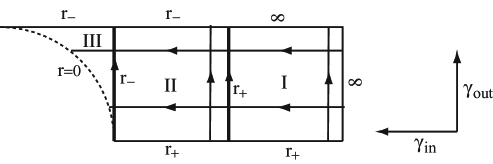
Figure 1: Kerr-Star space $M^{*}$.   Horizontal lines crossing the horizons represent ingoing null geodesics, while vertical lines outgoing null geodesics. Ingoing null geodesics run from $r=\infty$ to $r=0$. Outgoing null geodesics in the Boyer-Lindquist block I(III) run from $r=r_{+}$ ($r=0$) to $r=\infty$ ($r=r_{-}$); the radial coordinate increases since $\Delta_{r}>0$. In the block II, outgoing null geodesics run from $r=r_{+}$ to $r=r_{-}$; the radial coordinate decreases since $\Delta_{r}<0$.

The outgoing null geodesic $\gamma_{\rm out}$ is not defined on $H$. However, multiplying the factor $r^{2}\Delta_{r}/2$ with the right hand side in (4.12), we have a vector field

$$X^{*} = \frac{r^{2}\Delta_{r}}{2}\frac{\partial}{\partial r^{*}}+V~{},$$ (4.14)

which is defined on $M^{*}$ including $H$. Thus, one may understand the outgoing null geodesic $\gamma_{\rm out}$ as an integral curve of $X^{*}$. On the surface $r=$constant, the determinant of $g^{*}_{BH}|_{r={\rm const.}}$ is calculated as $-\rho^{2}r^{2}\Delta_{r}\sin^{2}\theta\cos^{2}\theta$, so that the restricted metric is degenerate if $\Delta_{r}=0$, i.e. the horizons $H_{\pm}=H|_{r=r_{\pm}}$ are null hypersurfaces. At $H_{\pm}$, $X^{*}$ in (4.14) reduces to the Killing vector fields

$$V_{\pm} = V|_{r=r_{\pm}}=(r_{\pm}^{2}+a^{2})(r_{\pm}^{2}+b^{2})\frac{\partial}{\partial t}+a(r_{\pm}^{2}+b^{2})\frac{\partial}{\partial\phi}+b(r_{\pm}^{2}+a^{2})\frac{\partial}{\partial\psi}~{}.$$ (4.15)

The vector fields $V_{\pm}$ are tangential to $H_{\pm}$ and also perpendicular to $H_{\pm}$. The integral curves of $V_{\pm}$ generate the horizons, which become totally geodesic null hypersurfaces in $M^{*}$.

If we introduce a coordinate (Star-Kerr coordinate),

$${}^{*}\!t=t-T(r)~{},~{}~{}~{}^{*}\!\phi=\phi-A(r)~{},~{}~{}~{}^{*}\!\psi=\psi-B(r)~{},~{}~{}~{}^{*}\!r=r~{},~{}~{}~{}^{*}\!\theta=\theta$$ (4.16)

instead of the Kerr-Star coordinate ($T$, $A$ and $B$ are the same functions as (4.8), (4.9) and (4.10)), the null geodesics are given by

$$\gamma^{\prime}_{\rm in} = -\frac{\partial}{\partial\,^{*}\!r}+\frac{2}{r^{2}\Delta_{r}}V(r)~{},$$ (4.17)

$$\gamma^{\prime}_{\rm out} = \frac{\partial}{\partial\,^{*}\!r}~{}.$$ (4.18)

Then, we obtain a metric

$$g_{BH} = \sum_{i,j=t,\phi,\psi}g_{ij}d\,^{*}\!x^{i}d\,^{*}\!x^{j}+g_{\theta\theta}d\theta^{2}-2d\,^{*}\!tdr+2a\sin^{2}\theta drd\,^{*}\!\phi+2b\cos^{2}\theta drd\,^{*}\psi~{},~{}~{}$$ (4.19)

which differs from (4.13) only in the last three terms. The Star-Kerr space ${}^{*}\!M={\mathbb{R}}_{+}^{2}\times$S³ is related to the Kerr-Star space $M^{*}$ by the following isometric mapping $f:{}^{*}\!M\to M^{*}$; ${}^{*}\!t=-t^{*},~{}^{*}\!\phi=-\phi^{*},~{}^{*}\!\psi=-\psi^{*}$ together with ${}^{*}\!r=r^{*}$ and ${}^{*}\!\theta=\theta^{*}$ (see figure 2).

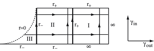
Figure 2: Star-Kerr space ${}^{*}\!M$.   Horizontal lines crossing the horizons represent outgoing null geodesics, while vertical lines ingoing null geodesics. Star-Kerr space is opposite to the Kerr-Star space in these respects.

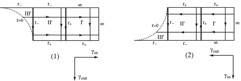
Figure 3: Kerr-Star^′ space and Star-Kerr^′ space.    Kerr-Star^′ space (1) (Star-Kerr^′ space (2)) is defined by reversing the directions of ingoing and outgoing null geodesics of Kerr-Star space (Star-Kerr space, respectively).

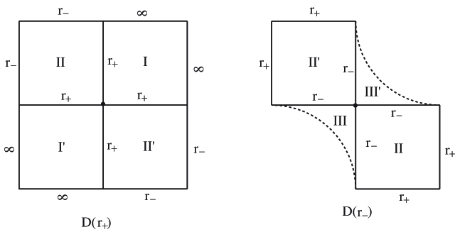
Figure 4: Kruskal spaces $D(r_{\pm})$.

Kruskal spaces $D(r_{\pm})$ are building blocks of the maximal extension (see figure 5). Dot $\bullet$ at the center represents the crossing three-sphere S${}^{3}(r_{\pm})$.

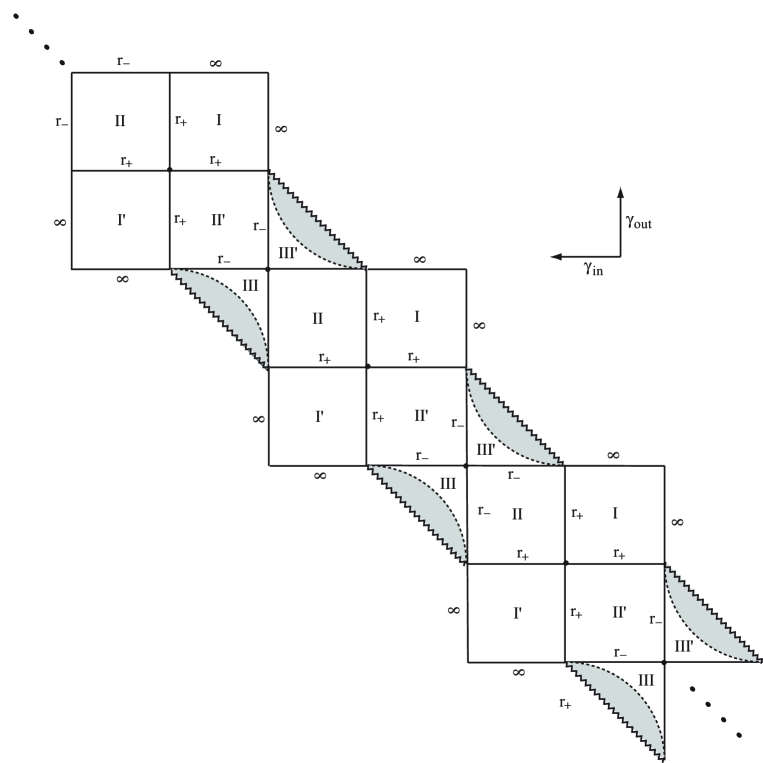
Figure 5: Maximal extension.   Each row corresponds to a Kerr-Star$(^{\prime})$ space while each column a Star-Kerr$(^{\prime})$ space. The Boyer-Lindquist block III (or III^′) is extended to a negative region of the square of radial coordinate $r^{2}$ [6], which is depicted in gray. The wavy lines in III (or III^′) represent curvature singularities defined by $r^{2}=-a^{2}\sin^{2}\theta-b^{2}\cos^{2}\theta$.

We may write the black hole metric in terms of the Kruskal coordinates $(u^{\pm},v^{\pm},\phi^{\pm},\psi^{\pm},\theta)$. These coordinates are defined on the regions $D(r_{\pm})$ (see figures 3, 4 and 5); the relation between Boyer-Lindquist and Kruskal coordinates are given by

$$|u^{\pm}| = \exp[\kappa_{\pm}(T(r)-t)]~{},$$ (4.20)

$$|v^{\pm}| = \exp[\kappa_{\pm}(T(r)+t)]~{},$$ (4.21)

$$\phi^{\pm} = \phi-\frac{at}{r_{\pm}^{2}+a^{2}}~{},$$ (4.22)

$$\psi^{\pm} = \psi-\frac{bt}{r_{\pm}^{2}+b^{2}},$$ (4.23)

where the constants

$$\kappa_{\pm}=\frac{r_{\pm}(r_{\pm}^{2}-r_{\mp}^{2})}{(r_{\pm}^{2}+a^{2})(r_{\pm}^{2}+b^{2})}$$ (4.24)

are the surface gravities of the horizons $H_{\pm}$. The integral (4.8) is calculated as

$$T(r)=r+\frac{1}{2\kappa_{+}}\log\left|\frac{r-r_{+}}{r+r_{+}}\right|+\frac{1}{2\kappa_{-}}\log\left|\frac{r-r_{-}}{r+r_{-}}\right|~{}.$$ (4.25)

Then the radial coordinate $r=r(u^{\pm}v^{\pm})$ is given implicitly by

$$u^{\pm}v^{\pm}=\frac{1}{G_{\pm}(r)}\left(\frac{r-r_{\pm}}{r+r_{\pm}}\right),$$ (4.26)

where

$$G_{\pm}(r)=\pm\left|\frac{r-r_{\mp}}{r+r_{\mp}}\right|^{r_{\mp}/r_{\pm}}\exp(-2\kappa_{\pm}r)$$ (4.27)

are non-zero analytic functions on $D(r_{\pm})$. Note that two hypersurfaces $u^{\pm}=0$ and $v^{\pm}=0$ express the horizons, which cross at the region $D(r_{\pm})|_{u_{\pm}=v_{\pm}=0}\simeq S^{3}(r_{\pm})$ (crossing three-sphere). The Killing vector fields $V_{\pm}$ on the horizons become

$$V_{\pm}=\kappa_{\pm}(r_{\pm}^{2}+a^{2})(r_{\pm}^{2}+b^{2})\left(-u^{\pm}\frac{\partial}{\partial u^{\pm}}+v^{\pm}\frac{\partial}{\partial v^{\pm}}\right)$$ (4.28)

in the Kruskal coordinate. It follows that the crossing spheres are fixed sets of $V_{\pm}$.

On $D(r_{+})$ the metric takes the form,

$$g_{BH} = \frac{G_{+}^{2}}{4\kappa_{+}^{2}}\frac{(r+r_{+})^{3}(r^{2}-r_{-}^{2})}{(r-r_{+})r^{2}\rho^{2}}\left(\frac{r^{4}\rho^{4}}{(r^{2}+a^{2})^{2}(r^{2}+b^{2})^{2}}-\frac{r_{+}^{4}\rho_{+}^{4}}{(r_{+}^{2}+a^{2})^{2}(r_{+}^{2}+b^{2})^{2}}\right)$$ (4.29)

$$~{}~{}~{}~{}~{}\times(u^{+2}dv^{+2}+v^{+2}du^{+2})$$

$$+\frac{G_{+}}{2\kappa_{+}^{2}}\frac{(r+r_{+})^{2}(r^{2}-r_{-}^{2})}{r^{2}\rho^{2}}\left(\frac{r^{4}\rho^{4}}{(r^{2}+a^{2})^{2}(r^{2}+b^{2})^{2}}+\frac{r_{+}^{4}\rho_{+}^{4}}{(r_{+}^{2}+a^{2})^{2}(r_{+}^{2}+b^{2})^{2}}\right)du^{+}dv^{+}$$

$$+\frac{G_{+}^{2}}{4\kappa_{+}^{2}}\frac{(r+r_{+})^{4}(a^{2}b^{2}\rho_{+}^{4}+a^{2}(r_{+}^{2}+b^{2})^{2}r^{2}\sin^{2}\theta+b^{2}(r_{+}^{2}+a^{2})^{2}r^{2}\cos^{2}\theta)}{r^{2}\rho^{2}(r_{+}^{2}+a^{2})^{2}(r_{+}^{2}+b^{2})^{2}}$$

$$~{}~{}~{}~{}~{}\times(u^{+}dv^{+}-v^{+}du^{+})^{2}$$

$$+\frac{aG_{+}}{\kappa_{+}}\frac{(r+r_{+})^{2}(r^{2}+a^{2}+\rho_{+}^{2})}{\rho^{2}(r_{+}^{2}+a^{2})}\sin^{2}\theta d\phi^{+}(u^{+}dv^{+}-v^{+}du^{+})$$

$$+\frac{bG_{+}}{\kappa_{+}}\frac{(r+r_{+})^{2}(r^{2}+b^{2}+\rho_{+}^{2})}{\rho^{2}(r_{+}^{2}+b^{2})}\cos^{2}\theta d\psi^{+}(u^{+}dv^{+}-v^{+}du^{+})$$

$$+g_{S^{3}(r_{+})}~{},$$

where $\rho_{+}^{2}=r_{+}^{2}+a^{2}\cos^{2}\theta+b^{2}\sin^{2}\theta$ and the last term

$$g_{S^{3}(r_{+})}=\sum_{i,j=\phi^{+},\psi^{+}}~{}g_{ij}dx^{i}dx^{j}+\rho^{2}d\theta^{2}~{},$$ (4.30)

($g_{ij}$ are the same functions as (3.5)-(3.7)) gives a metric on the crossing sphere $S^{3}(r_{+})$. In this coordinate, $S^{3}(r_{+})$ becomes a totally geodesic submanifold of $D(r_{+})$. The metric on $D(r_{-})$ is given by replacing plus indices with minus indices. If we put $a=b=0$ (Schwarzschild metric), for which we have $r_{+}=1/\kappa_{+}=\sqrt{2m}$ and $r_{-}=0$, then the metric reduces to

$$g_{BH}=2m\left(1+\frac{\sqrt{2m}}{r}\right)^{2}\exp\left(-\sqrt{\frac{2}{m}}r\right)du^{+}dv^{+}+r^{2}(d\theta^{2}+\sin^{2}\theta d\phi^{2}+\cos^{2}\theta d\psi^{2})~{}$$

with

$$u^{+}v^{+}=\left(\frac{r-\sqrt{2m}}{r+\sqrt{2m}}\right)\exp\left(\sqrt{\frac{2}{m}}r\right).$$ (4.32)

5 Five-dimensional AdS Kerr black holes

The analysis persists in the case with a cosmological constant. The AdS Kerr metric in the Boyer-Lindquist coordinate is given as [7]

$$g_{BH}^{\prime} = -\frac{\Delta_{r}}{\rho^{2}}\left[dt-\frac{a\sin^{2}\theta}{\Xi_{a}}d\phi-\frac{b\cos^{2}\theta}{\Xi_{b}}d\psi\right]^{2}+\frac{\rho^{2}}{\Delta_{r}}dr^{2}+\frac{\rho^{2}}{\Delta_{\theta}}d\theta^{2}$$ (5.1)

$$+\frac{\Delta_{\theta}\sin^{2}\theta}{\rho^{2}}(adt-\frac{r^{2}+a^{2}}{\Xi_{a}}d\phi)^{2}+\frac{\Delta_{\theta}\cos^{2}\theta}{\rho^{2}}(bdt-\frac{r^{2}+b^{2}}{\Xi_{b}}d\psi)^{2}$$

$$+\frac{1+r^{2}\ell^{2}}{r^{2}\rho^{2}}\left[abdt-\frac{b(r^{2}+a^{2})\sin^{2}\theta}{\Xi_{a}}d\phi-\frac{a(r^{2}+b^{2})\cos^{2}\theta}{\Xi_{b}}d\psi\right]^{2}~{},$$

where

$$\rho^{2}=r^{2}+a^{2}\cos^{2}\theta+b^{2}\sin^{2}\theta~{},~{}~{}~{}\Delta_{r}=\frac{1}{r^{2}}(r^{2}+a^{2})(r^{2}+b^{2})(1+r^{2}\ell^{2})-2m~{},$$

$$\Delta_{\theta}=1-a^{2}\ell^{2}\cos^{2}\theta-b^{2}\ell^{2}\sin^{2}\theta~{},~{}~{}~{}\Xi_{a}=1-a^{2}\ell^{2}~{},~{}~{}~{}\Xi_{b}=1-b^{2}\ell^{2}~{}.$$ (5.2)

We find that the theorem 1 is generalized as follows.

Theorem 2.
There exists a constant $K^{\prime}$ for a geodesic $\gamma$ satisfying

$${\rho^{4}}\left(\frac{d\theta}{ds}\right)^{2}+\Theta_{\ell}(\theta)=0~{},$$ (5.3)

$${\rho^{4}}\left(\frac{dr}{ds}\right)^{2}+R_{\ell}(r)=0~{},$$ (5.4)

where

$$\Theta_{\ell} = (a^{2}\sin^{2}\theta+b^{2}\cos^{2}\theta-a^{2}b^{2}\ell^{2})L_{t}^{2}+\frac{\Xi_{a}^{2}(1-b^{2}\ell^{2}\sin^{2}\theta)}{\sin^{2}\theta}L_{\phi}^{2}+\frac{\Xi_{b}^{2}(1-a^{2}\ell^{2}\cos^{2}\theta)}{\cos^{2}\theta}L_{\psi}^{2}$$ (5.5)

$$-2\ell^{2}\left(a^{2}\sin^{2}\theta+b^{2}\cos^{2}\theta-a^{2}b^{2}\ell^{2}\right)L_{t}(aL_{\phi}+bL_{\psi})-2ab\ell^{2}\Xi_{a}\Xi_{b}L_{\phi}L_{\psi}$$

$$-\Delta_{\theta}(a^{2}\cos^{2}\theta+b^{2}\sin^{2}\theta)Q-\Delta_{\theta}K^{\prime}~{},$$

$$R_{\ell} = R_{-2}r^{-2}+R_{0}+R_{2}r^{2}+R_{4}r^{4}+R_{6}r^{6}~{}.$$ (5.6)

The coefficients are explicitly given by

$$R_{6} = -Q\ell^{2}~{},$$ (5.7)

$$R_{4} = -L_{t}^{2}+2\ell^{2}L_{t}(aL_{\phi}+bL_{\psi})-(1+a^{2}\ell^{2}+b^{2}\ell^{2})Q+\ell^{2}K^{\prime}~{},$$ (5.8)

$$R_{2} = \left(-2(a^{2}+b^{2})+a^{2}b^{2}\ell^{2}\right)L_{t}\left(L_{t}-2\ell^{2}(aL_{\phi}+bL_{\psi})\right)+2ab\ell^{2}\Xi_{a}\Xi_{b}L_{\phi}L_{\psi}$$ (5.9)

$$+b^{2}\ell^{2}\Xi_{a}^{2}L_{\phi}^{2}+a^{2}\ell^{2}\Xi_{b}^{2}L_{\psi}^{2}-(a^{2}+b^{2}+a^{2}b^{2}\ell^{2}-2m)Q+(1+a^{2}\ell^{2}+b^{2}\ell^{2})K^{\prime}~{},$$

$$R_{0} = (-a^{4}\Xi_{b}-b^{4}\Xi_{a}-3a^{2}b^{2})L_{t}^{2}+\Xi_{a}^{2}(b^{2}-a^{2}+a^{2}b^{2}\ell^{2}+b^{4}\ell^{2})L_{\phi}^{2}$$ (5.10)

$$+\Xi_{b}^{2}(a^{2}-b^{2}+a^{2}b^{2}\ell^{2}+a^{4}\ell^{2})L_{\psi}^{2}-2ab\ell^{2}\Xi_{a}\Xi_{b}(a^{2}+b^{2})L_{\phi}L_{\psi}$$

$$+2\left(a^{4}\ell^{2}\Xi_{b}+b^{4}\ell^{4}\Xi_{a}+3a^{2}b^{2}\ell^{2}-2m\right)L_{t}(aL_{\phi}+bL_{\psi})$$

$$-a^{2}b^{2}Q+(a^{2}+b^{2}+a^{2}b^{2}\ell^{2}-2m)K^{\prime}~{},$$

$$R_{-2} = -a^{2}b^{2}(a^{2}+b^{2}-a^{2}b^{2}\ell^{2}+2m)L_{t}^{2}-b^{2}\Xi_{a}^{2}(a^{2}\Xi_{b}^{2}-b^{2}+2m)L_{\phi}^{2}$$ (5.11)

$$-a^{2}\Xi_{b}^{2}(b^{2}\Xi_{a}^{2}-a^{2}+2m)L_{\psi}^{2}+2ab^{2}\left(a^{2}\ell^{2}(a^{2}\Xi_{b}+b^{2})+2m\Xi_{a}\right)L_{t}L_{\phi}+a^{2}b^{2}K^{\prime}$$

$$+2a^{2}b\left(b^{2}\ell^{2}(b^{2}\Xi_{a}+a^{2})+2m\Xi_{b}\right)L_{t}L_{\psi}+2ab\Xi_{a}\Xi_{b}(a^{2}b^{2}\ell^{2}-2m)L_{\phi}L_{\psi}~{}$$

with

$$Q=\langle\gamma^{\prime},\gamma^{\prime}\rangle~{},~{}~{}~{}L_{i}=\langle\gamma^{\prime},\frac{\partial}{\partial x^{i}}\rangle,~{}~{}~{}x^{i}=(t,\phi,\psi).$$ (5.12)

These equations reduce to (3.13) and (3.14) when we set $\ell=0$.

The special geodesics in (4.2) are generalized to

$$\gamma^{\prime}_{\{\rm{out\atop in}} = \pm\frac{\partial}{\partial r}+\frac{1}{r^{2}\Delta_{r}}V(r)$$ (5.13)

with

$$V(r) = (r^{2}+a^{2})(r^{2}+b^{2})\frac{\partial}{\partial t}+a\Xi_{a}(r^{2}+b^{2})\frac{\partial}{\partial\phi}+b\Xi_{b}(r^{2}+a^{2})\frac{\partial}{\partial\psi}~{}.$$ (5.14)

The constants are

$$Q=0~{},~{}~{}~{}L_{t}=-1~{},~{}~{}~{}L_{\phi}=\frac{a\sin^{2}\theta}{\Xi_{a}}~{},~{}~{}~{}L_{\psi}=\frac{b\cos^{2}\theta}{\Xi_{b}}~{},$$

$$K=\frac{2}{\Xi_{a}\Xi_{b}}(a^{2}\sin^{2}\theta+b^{2}\cos^{2}\theta-a^{2}b^{2}\ell^{2})~{},$$ (5.15)

for which we have $\Theta_{\ell}=0$ and $R_{\ell}=-\rho^{4}$.

In the same way as the Ricci flat case, Kerr-Star coordinate and Star-Kerr coordinate are introduced:

$${{}^{*}\!t}^{*}=t\pm T(r)~{},~{}~{}~{}^{*}\!\phi^{*}=\phi\pm A(r)~{},~{}~{}~{}^{*}\!\psi^{*}=\psi\pm B(r)~{},~{}~{}$$ (5.16)

where

$$T(r) = \int\frac{(r^{2}+a^{2})(r^{2}+b^{2})}{r^{2}\Delta_{r}}dr~{},$$ (5.17)

$$A(r) = \int\frac{a\Xi_{a}(r^{2}+b^{2})}{r^{2}\Delta_{r}}dr~{},$$ (5.18)

$$B(r) = \int\frac{b\Xi_{b}(r^{2}+a^{2})}{r^{2}\Delta_{r}}dr~{}.$$ (5.19)

Then, the metric is given by

$$g_{BH}^{\prime} = \sum_{i,j=t,\phi,\psi}g_{ij}d\,^{*}\!x^{*i}d\,^{*}\!x^{*j}+g_{\theta\theta}d\theta^{2}\mp 2d\,^{*}\!t^{*}dr\pm\frac{2a\sin^{2}\theta}{\Xi_{a}}drd\,^{*}\!\phi^{*}\pm\frac{2b\cos^{2}\theta}{\Xi_{b}}drd\,^{*}\psi^{*}~{},$$

where

$$g_{tt} = -1+\frac{2m}{\rho^{2}}-\ell^{2}(r^{2}+a^{2}\sin^{2}\theta+b^{2}\cos^{2}\theta)~{},$$ (5.21)

$$g_{t\phi} = -\frac{2ma\sin^{2}\theta}{\rho^{2}\Xi_{a}}+\ell^{2}\frac{a\sin^{2}\theta}{\Xi_{a}}(r^{2}+a^{2})~{},$$ (5.22)

$$g_{t\psi} = -\frac{2mb\cos^{2}\theta}{\rho^{2}\Xi_{b}}+\ell^{2}\frac{b\cos^{2}\theta}{\Xi_{b}}(r^{2}+b^{2})~{},$$ (5.23)

$$g_{\phi\phi} = \sin^{2}\theta\left[\frac{r^{2}+a^{2}}{\Xi_{a}}+\frac{2\sin^{2}\theta a^{2}m}{\rho^{2}\Xi_{a}^{2}}\right]~{},$$ (5.24)

$$g_{\psi\psi} = \cos^{2}\theta\left[\frac{r^{2}+b^{2}}{\Xi_{b}}+\frac{2\cos^{2}\theta b^{2}m}{\rho^{2}\Xi_{b}^{2}}\right]~{},$$ (5.25)

$$g_{\phi\psi} = \frac{2abm\cos^{2}\theta\sin^{2}\theta}{\rho^{2}\Xi_{a}\Xi_{b}}~{}.$$ (5.26)

In this coordinate system, the special geodesics (5.13) reduce to (4.17) and (4.18), or (4.11) and (4.12), with $V$ in (5.14) and $\Delta_{r}$ in (5.2).

We now describe some curvature property of the AdS Kerr black hole. Let us introduce an orthonormal frame $\{e_{a}\}$ $(a=1,...,5)$:

$$e_{1} = \frac{1}{r^{2}\sqrt{\Delta_{r}\varepsilon}\rho}V~{},$$ (5.27)

$$e_{2} = \frac{\Xi_{a}\Xi_{b}}{\Omega_{2}\sin\theta}\left(\frac{\hat{\Sigma}_{b}}{\Xi_{b}}W+\frac{b\hat{\Sigma}_{a}}{F}Z\right)~{},$$ (5.28)

$$e_{3} = \frac{\Xi_{a}\Xi_{b}}{\Omega_{3}\cos\theta}\left(\frac{\hat{\Sigma}_{a}}{\Xi_{a}}W-\frac{a\hat{\Sigma}_{b}}{F}Z\right)~{},$$ (5.29)

$$e_{4} = \frac{\sqrt{\Delta_{r}\varepsilon}}{\rho}\frac{\partial}{\partial r}~{},$$ (5.30)

$$e_{5} = \frac{\sqrt{\Delta_{\theta}}}{\rho}\frac{\partial}{\partial\theta}~{}.$$ (5.31)

The vector field $V$ is given by (5.14), and

$$W = \frac{a}{\Xi_{a}}\sin^{2}\theta\frac{\partial}{\partial t}+\frac{\partial}{\partial\phi}~{},$$ (5.32)

$$Z = \frac{a}{\Xi_{a}}\sin^{2}\theta\frac{\partial}{\partial\psi}-\frac{b}{\Xi_{b}}\cos^{2}\theta\frac{\partial}{\partial\phi}~{},$$ (5.33)

which satisfy $\langle V,W\rangle=\langle V,Z\rangle=0$. The functions $\hat{\Sigma}_{a}$, $\hat{\Sigma}_{b}$ and $F$ are defined by

$$\hat{\Sigma}_{a}=\sqrt{r^{2}+\frac{\Delta_{\theta}}{\Xi_{a}}a^{2}}~{},~{}~{}~{}\hat{\Sigma}_{b}=\sqrt{r^{2}+\frac{\Delta_{\theta}}{\Xi_{b}}b^{2}}~{},$$ (5.34)

and

$$F = \frac{1}{1-\ell^{2}\rho^{2}}\left(\frac{1}{2}(\Xi_{a}+\Xi_{b})\hat{\Sigma}_{a}\hat{\Sigma}_{b}+\sqrt{\Delta_{\theta}r^{2}\rho^{2}+\frac{1}{4}\ell^{4}(a^{2}-b^{2})^{2}\hat{\Sigma}_{a}^{2}\hat{\Sigma}_{b}^{2}}\right)~{},$$ (5.35)

with

$$(\Omega_{2})^{2} = \hat{\Sigma}_{b}^{2}r^{2}+(a^{2}\hat{\Sigma}_{b}^{2}-b^{2}\hat{\Sigma}_{a}^{2})(1-\ell^{2}\rho^{2})\cos^{2}\theta-b^{2}\hat{\Sigma}_{a}^{3}\hat{\Sigma}_{b}(\Xi_{a}-\Xi_{b})\frac{\cos^{2}\theta}{F}~{},$$ (5.36)

$$(\Omega_{3})^{2} = \hat{\Sigma}_{a}^{2}r^{2}-(a^{2}\hat{\Sigma}_{b}^{2}-b^{2}\hat{\Sigma}_{a}^{2})(1-\ell^{2}\rho^{2})\sin^{2}\theta+a^{2}\hat{\Sigma}_{a}\hat{\Sigma}_{b}^{3}(\Xi_{a}-\Xi_{b})\frac{\sin^{2}\theta}{F}~{}.$$ (5.37)

If we put $\ell=0$, the equations (5.27)-(5.31) reduce to (2.11)-(2.15). We consider the Weyl curvature $W^{ab}{}_{cd}$ as a linear map on two forms. The corresponding matrix $\hat{W}^{ab}{}_{cd}$ defined by $W^{ab}{}_{cd}=\frac{2m}{\rho^{6}}\hat{W}^{ab}{}_{cd}$ takes the form (2.40). Note that the functions I and J defined in (2.41) are replaced with $\hat{\rm\bf I}$ and $\hat{\rm\bf J}$, respectively, as

$$\hat{\rm\bf I} = \frac{a\cos\theta}{r}\frac{(\hat{\Sigma}_{b}F-b^{2}\hat{\Sigma}_{a})\sqrt{\Delta_{\theta}}\rho}{F\Omega_{2}}~{},~{}~{}~{}\hat{\rm\bf J}=\frac{b\sin\theta}{r}\frac{(\hat{\Sigma}_{a}F-a^{2}\hat{\Sigma}_{b})\sqrt{\Delta_{\theta}}\rho}{F\Omega_{3}}~{}.$$ (5.38)

In general, they depend on the cosmological constant $\ell$, but the combination $\hat{\rm\bf K}^{2}\equiv\hat{\rm\bf I}^{2}+\hat{\rm\bf J}^{2}$ coincides with ${\rm\bf K}^{2}={\rm\bf I}^{2}+{\rm\bf J}^{2}$, i.e. $\hat{\rm\bf K}^{2}={\rm\bf K}^{2}$. As special cases, we have $\hat{\rm\bf I}={\rm\bf I}$ and $\hat{\rm\bf J}={\rm\bf J}$ for $a=b$ or $a\neq 0,b=0$ ($a=0,b\neq 0$). We find that the eigenvalues are exactly the same as (2.42)-(LABEL:lambda_6). Thus we state as follows.

Theorem 3.
Five-dimensional AdS Kerr black holes are isospectrum deformations of Ricci-flat Kerr black holes in the sense that the eigenvalues of the Weyl curvature are preserved.

Remark 1.
We conjecture that the statement above is true for the general AdS Kerr black holes in all dimensions [4] (see appendix A for AdS Kerr black holes in four-dimensions).

Remark 2.
Changing the negative cosmological constant to the positive one, $\ell^{2}\to-\ell^{2}$, we obtain the same results.

Finally we discuss the relation between the Weyl curvature of AdS Kerr black holes with equal angular momenta $a=b$ and that of Sasaki-Einstein metrics constructed in [14]. According to [15] [5], we write the five-dimensional AdS black hole metric with a negative cosmological constant $4\Lambda$ as

$$g = -\frac{W(R)}{b(R)}dt^{2}+\frac{dR^{2}}{W(R)}+R^{2}\left(\frac{1}{4}(d\theta^{2}+\sin^{2}\theta d\phi^{2})+b(R)\left(d\psi+\frac{1}{2}\cos\theta d\phi+f(R)dt\right)^{2}\right),$$

where

$$W = 1-\Lambda R^{2}-\frac{2m(\delta^{2}+\Lambda J^{2})}{R^{2}}+\frac{2mJ^{2}}{R^{4}}~{},$$

$$b = 1+\frac{2mJ^{2}}{R^{4}}~{},~{}~{}~{}f=\frac{1}{J}\left(1-\frac{\delta}{b}\right)~{}.$$ (5.40)

The metric is parameterized by the mass $m$, the angular momentum $J$ and an unphysical parameter $\delta$ [15]. The eigenvalues of the Weyl curvature are calculated in the same way;

$$2 ~{}:~{} \lambda_{1}=\frac{2m}{R^{4}}(\delta^{2}+\Lambda J^{2})~{},$$ (5.41)

$$2 ~{}:~{} \lambda_{2}=-\frac{2m}{R^{4}}(\delta^{2}+\Lambda J^{2})~{},$$ (5.42)

$$2 ~{}:~{} \lambda_{3}=\frac{2m}{R^{6}}\left(2J^{2}-(\delta^{2}+\Lambda J^{2})R^{2}+2J\sqrt{J^{2}-(\delta^{2}+\Lambda J^{2})R^{2})}\right)~{},$$ (5.43)

$$2 ~{}:~{} \lambda_{4}=\frac{2m}{R^{6}}\left(2J^{2}-(\delta^{2}+\Lambda J^{2})R^{2}-2J\sqrt{J^{2}-(\delta^{2}+\Lambda J^{2})R^{2})}\right)~{},$$ (5.44)

$$1 ~{}:~{} \lambda_{5}=\frac{2m}{R^{6}}\left(-4J^{2}+2(\delta^{2}+\Lambda J^{2})R^{2}-\sqrt{16J^{4}-16J^{2}(\delta^{2}+\Lambda J^{2})R^{2}+(\delta^{2}+\Lambda J^{2})^{2}R^{4}}\right)~{},$$

$$1 ~{}:~{} \lambda_{6}=\frac{2m}{R^{6}}\left(-4J^{2}+2(\delta^{2}+\Lambda J^{2})R^{2}+\sqrt{16J^{4}-16J^{2}(\delta^{2}+\Lambda J^{2})R^{2}+(\delta^{2}+\Lambda J^{2})^{2}R^{4}}\right)~{},$$

where the number in the left hand side represents the degeneracy. If we introduce a new radial coordinate $r$ defined by

$$R^{2}=\sqrt{\delta^{2}+\Lambda J^{2}}\left(r^{2}+\frac{J^{2}}{(\delta^{2}+\Lambda J^{2})^{3/2}}\right),$$ (5.47)

then the eigenvalues reduce to (2.42)-(LABEL:lambda_6) with

$$a^{2}=b^{2}=\frac{J^{2}}{(\delta^{2}+\Lambda J^{2})^{3/2}}~{}.$$ (5.48)

The Sasaki-Einstein metric appears by setting $\delta^{2}+\Lambda J^{2}=0$ (together with an Wick rotation) as shown in [5]. Then the equations (5.41)-(LABEL:lambda_6:_twist) yield

$$\lambda_{1}=\lambda_{2}=\lambda_{4}=\lambda_{6}=0~{},~{}~{}~{}\lambda_{3}=\frac{8mJ^{2}}{R^{6}}~{},~{}~{}~{}\lambda_{5}=-\frac{16mJ^{2}}{R^{6}}~{},$$ (5.49)

so that the multiplicity changes at this special value of $\delta$. Note that from (5.47) and (5.48) this setting is not allowed in the parameterization of the metric (5.1).

Appendix A Four-dimensional AdS Kerr black holes

In this appendix, we briefly describe geodesics and the Weyl curvature of four-dimensional AdS Kerr black holes.

The metric with a negative cosmological constant $-3\ell^{2}$ is given as

$$g_{BH}^{(4)}=-\frac{\Delta_{r}}{\rho^{2}}\left(dt-\frac{a}{\Xi}\sin^{2}\theta d\phi\right)^{2}+\frac{\rho^{2}}{\Delta_{r}}dr^{2}+\frac{\rho^{2}}{\Delta_{\theta}}d\theta^{2}+\frac{\sin^{2}\theta\Delta_{\theta}}{\rho^{2}}\left(adt-\frac{r^{2}+a^{2}}{\Xi}d\phi\right)^{2},~{}~{}~{}~{}~{}~{}$$ (A.1)

where

$$\rho^{2}=r^{2}+a^{2}\cos^{2}\theta~{},~{}~{}~{}\Delta_{r}=(r^{2}+a^{2})(1+\ell^{2}r^{2})-2mr~{},$$

$$\Delta_{\theta}=1-\ell^{2}a^{2}\cos^{2}\theta~{},~{}~{}~{}\Xi=1-\ell^{2}a^{2}~{},$$ (A.2)

which is parameterized by the mass $m$ and the angular momentum $a$. The orthonormal frame $\{e_{a}\}$ $(a=1,2,3,4)$ is given as

$$e_{1} = \frac{1}{\sqrt{\Delta_{r}}\rho}\left((r^{2}+a^{2})\frac{\partial}{\partial t}+a\Xi\frac{\partial}{\partial\phi}\right)~{},$$ (A.3)

$$e_{2} = \frac{1}{\sqrt{\Delta_{\theta}}\rho\sin\theta}\left(a\sin^{2}\theta\frac{\partial}{\partial t}+\Xi\frac{\partial}{\partial\phi}\right)~{},$$ (A.4)

$$e_{3} = \frac{\sqrt{\Delta_{r}}}{\rho}\frac{\partial}{\partial r}~{},$$ (A.5)

$$e_{4} = \frac{\sqrt{\Delta_{\theta}}}{\rho}\frac{\partial}{\partial\theta}~{}.$$ (A.6)

The four-dimensional version of the theorem 2 states as follows. There exists a constant $K^{\prime}$ for a geodesic $\gamma$ satisfying

$$\rho^{4}\left(\frac{d\theta}{ds}\right)^{2}+\Theta_{\ell}(\theta)=0~{},~{}~{}~{}\rho^{4}\left(\frac{dr}{ds}\right)^{2}+R_{\ell}(r)=0~{},$$ (A.7)

where

$$\Theta_{\ell} = a^{2}\sin^{2}\theta L_{t}^{2}+\frac{\Xi^{2}}{\sin^{2}\theta}L_{\phi}^{2}+2a\Xi L_{t}L_{\phi}-a^{2}\cos^{2}\theta\Delta_{\theta}Q-\Delta_{\theta}K^{\prime}~{},$$ (A.8)

$$R_{\ell} = R_{0}+R_{1}r+R_{2}r^{2}+R_{3}r^{3}+R_{4}r^{4}+R_{6}r^{6}~{}.$$ (A.9)

The coefficients are explicitly given as

$$R_{6} = -Q\ell^{2}~{},$$ (A.10)

$$R_{4} = -L_{t}^{2}-(1+a^{2}\ell^{2})Q+\ell^{2}K^{\prime}~{},$$ (A.11)

$$R_{3} = 2m~{},$$ (A.12)

$$R_{2} = -2a^{2}L_{t}^{2}-2a\Xi L_{t}L_{\phi}-a^{2}Q+(1+a^{a}\ell^{2})K^{\prime}~{},$$ (A.13)

$$R_{1} = -2mK^{\prime}~{},$$ (A.14)

$$R_{0} = a^{2}(-a^{2}L_{t}^{2}-\Xi^{2}L_{\phi}^{2}-2a\Xi L_{t}L_{\phi}+K^{\prime})~{},$$ (A.15)

with $Q=\langle\gamma^{\prime},\gamma^{\prime}\rangle,~{}L_{i}=\langle\gamma^{\prime},\frac{\partial}{\partial x^{i}}\rangle,~{}x^{i}=(t,\phi)$.

Next, we consider a linear map on two-forms defined by the Weyl curvature $W^{ab}{}_{cd}$. We find that the non-zero components of the matrix $\hat{W}^{ab}{}_{cd}$ with $W^{ab}{}_{cd}=\frac{2m}{\rho^{2}}\hat{W}^{ab}{}_{cd}$ are given as

$$\begin{array}[]{c|cccccc}(a,b)\setminus(c,d)&(1,2)&(1,3)&(1,4)&(2,3)&(2,4)&(4,5)\\ \hline\cr(1,2)&-{\rm\bf I}&&&&&-{\rm\bf J}\\ (1,3)&&2{\rm\bf I}&&&-2{\rm\bf J}&\\ (1,4)&&&-{\rm\bf I}&-{\rm\bf J}&&\\ (2,3)&&&{\rm\bf J}&-{\rm\bf I}&&\\ (2,4)&&2{\rm\bf J}&&&2{\rm\bf I}&\\ (3,4)&{\rm\bf J}&&&&&-{\rm\bf I}\\ \end{array}$$ (A.23)

where ${\rm\bf I}$ and ${\rm\bf J}$ are defined as

$${\rm\bf I}=\frac{1}{2}r(r^{2}-3a^{2}\cos^{2}\theta)~{},~{}~{}~{}{\rm\bf J}=\frac{1}{2}a\cos\theta(3r^{2}-a^{2}\cos^{2}\theta)~{}.$$ (A.24)

It should be noted that this matrix is independent of $\ell$, and the same as the one examined in [8] for the Ricci-flat Kerr black hole. The eigenvalues are

$$2 ~{}:~{} \lambda_{1}=-{\rm\bf I}+i{\rm\bf J}~{},$$ (A.25)

$$2 ~{}:~{} \lambda_{2}=-{\rm\bf I}-i{\rm\bf J}~{},$$ (A.26)

$$1 ~{}:~{} \lambda_{3}=2{\rm\bf I}+2i{\rm\bf J}~{},$$ (A.27)

$$1 ~{}:~{} \lambda_{4}=2{\rm\bf I}-2i{\rm\bf J}~{},$$ (A.28)

where the number in the left hand side represents the degeneracy. Thus, the theorem 3 persists in four-dimensions; four-dimensional AdS Kerr black holes are isospectrum deformations of Ricci-flat Kerr black holes.

References

- [1] J. M. Maldacena, “The large N limit of superconformal field theories and supergravity,” Adv. Theor. Math. Phys. 2 (1998) 231 [Int. J. Theor. Phys. 38 (1999) 1113] [arXiv:hep-th/9711200]; S. S. Gubser, I. R. Klebanov and A. M. Polyakov, “Gauge theory correlators from non-critical string theory,” Phys. Lett. B 428 (1998) 105 [arXiv:hep-th/9802109]; E. Witten, “Anti-de Sitter space and holography,” Adv. Theor. Math. Phys. 2 (1998) 253 [arXiv:hep-th/9802150].
- [2] D. Page, “A Compact Rotating Gravitational Instanton,” Phys. Lett. B 79 (1978) 235.
- [3] Y. Hashimoto, M. Sakaguchi and Y. Yasui, “New infinite series of Einstein metrics on sphere bundles from AdS black holes,” Commun. Math. Phys. in press [arXiv:hep-th/0402199].
- [4] G. W. Gibbons, H. Lu, D. N. Page and C. N. Pope, “The general Kerr-de Sitter metrics in all dimensions,” J. Geom. Phys. 53 (2005) 49 [arXiv:hep-th/0404008]; “Rotating black holes in higher dimensions with a cosmological constant,” Phys. Rev. Lett. 93 (2004) 171102 [arXiv:hep-th/0409155].
- [5] Y. Hashimoto, M. Sakaguchi and Y. Yasui, “Sasaki-Einstein twist of Kerr-AdS black holes,” Phys. Lett. B 600 (2004) 270 [arXiv:hep-th/0407114].
- [6] R. C. Myers and M. J. Perry, “Black Holes In Higher Dimensional Space-Times,” Annals Phys. 172 (1986) 304.
- [7] S. W. Hawking, C. J. Hunter and M. M. Taylor-Robinson, “Rotation and the AdS/CFT correspondence,” Phys. Rev. D 59 (1999) 064005 [arXiv:hep-th/9811056].
- [8] B. O’Neill, “The Geometry of Kerr Black Holes,” A K Peters, Ltd., 1995.
- [9] V. P. Frolov and D. Stojkovic, “Particle and light motion in a space-time of a five-dimensional rotating black hole,” Phys. Rev. D 68 (2003) 064011 [arXiv:gr-qc/0301016].
- [10] P. J. De Smet, “The Petrov type of the five-dimensional Myers-Perry metric,” Gen. Rel. Grav. 36 (2004) 1501 [arXiv:gr-qc/0312021].
- [11] H. K. Kunduri and J. Lucietti, “Integrability and the Kerr-(A)dS black hole in five dimensions,” arXiv:hep-th/0502124.
- [12] A. N. Aliev and V. P. Frolov, “Five dimensional rotating black hole in a uniform magnetic field: The gyromagnetic ratio,” Phys. Rev. D 69 (2004) 084022 [arXiv:hep-th/0401095].
- [13] B. Carter, “Global Structure Of The Kerr Family Of Gravitational Fields,” Phys. Rev. 174 (1968) 1559.
- [14] J. P. Gauntlett, D. Martelli, J. Sparks and D. Waldram, “Sasaki-Einstein metrics on S(2) x S(3),” arXiv:hep-th/0403002.
- [15] M. Cvetic, H. Lu and C. N. Pope, “Charged Kerr-de Sitter black holes in five dimensions,” Phys. Lett. B 598 (2004) 273 [arXiv:hep-th/0406196].