Controlling Chaos through Compactification in
Cosmological Models with a Collapsing Phase

Abstract

We consider the effect of compactification of extra dimensions on the onset of classical chaotic “Mixmaster” behavior during cosmic contraction. Assuming a universe that is well–approximated as a four–dimensional Friedmann–Robertson–Walker model (with negligible Kaluza–Klein excitations) when the contraction phase begins, we identify compactifications that allow a smooth contraction and delay the onset of chaos until arbitrarily close to the big crunch. These compactifications are defined by the de Rham cohomology (Betti numbers) and Killing vectors of the compactification manifold. We find compactifications that control chaos in vacuum Einstein gravity, as well as in string theories with $\mathcal{N}=1$ supersymmetry and M–theory. In models where chaos is controlled in this way, the universe can remain homogeneous and flat until it enters the quantum gravity regime. At this point, the classical equations leading to chaotic behavior can no longer be trusted, and quantum effects may allow a smooth approach to the big crunch and transition into a subsequent expanding phase. Our results may be useful for constructing cosmological models with contracting phases, such as the ekpyrotic/cyclic and pre–big bang models.

I Introduction

The behavior of spacetime near a big crunch singularity has been a topic of research for many decades. The classic studies of Belinskii, Khalatnikov, and Lifshitz (BKL) Lif63 ; Bel70 ; Bel73 and others Dem85 ; Dam00 ; Dam00A ; Dam02 ; Dam02A ; Dam02B ; Mis69 ; MTW ; Cor97 have shown that the contraction to the crunch can proceed either smoothly or chaotically. Chaos arises when the universe is unstable to small inhomogeneities and anisotropies in curvature or matter fields. These “dangerous” perturbations grow and eventually dominate the dynamics, driving the universe to an anisotropic state, expanding along some axes and contracting along others. The axes and their rates of contraction jump to new values when new curvature or matter terms grow to dominate. The jumps generally repeat an infinite number of times before the big crunch itself. The chaotic, oscillatory evolution to the big crunch is often known as “Mixmaster” behavior or “BKL oscillations.”

Models that generalize four dimensional Einstein gravity have been classified by whether they necessarily exhibit chaotic behavior near a big crunch. This classification is established assuming “generic” initial conditions, in which there is a finite, but possibly small, energy density in all fields present in the model. Additionally, one assumes that the classical Einstein equations remain valid up to the big crunch itself. Under these assumptions, it has been shown that vacuum Einstein gravity in spacetime dimension less than eleven, as well as all uncompactified ten dimensional string theories and M–theory, will inevitably suffer chaos as the big crunch is approached Dem85 ; Dam00 ; Gib05 . So too will Einstein gravity containing only perfect fluids with equation of state $w<1$, where $w=p/\rho$ is the ratio of the fluid’s pressure to its energy density. On the other hand, there are cases where chaos is not inevitable. Among these are Einstein gravity with a free massless scalar field, leading to $w=1$, and a universe containing a perfect fluid with equation of state $w\geq 1$ Eri03 .

The presence of chaos during gravitational collapse is a potential problem for cosmological models with a big crunch/big bang transition, such as the ekpyrotic/cyclic and pre big–bang scenarios Kho01A ; Ste02 ; Ven00 ; Gas02 . In these models, the universe undergoes collapse to a big crunch, followed by a transition to the conventional big bang and subsequent expansion. It is assumed that, during the collapsing phase, the universe is nearly homogeneous and isotropic, with a scale invariant perturbation spectrum. BKL oscillations arising during the collapsing phase would destroy homogeneity and isotropy, producing a chaotic spacetime with structure down to arbitrarily small scales. In this situation, a big crunch/big bang transition is unlikely to be describable in a deterministic manner, and it is questionable whether a homogeneous and isotropic universe with the long range correlations required by observations could emerge Pee72 . Thus, avoiding chaos is an essential feature of cosmological models with a collapsing phase.

We take the point of view that avoiding chaos all the way to the the big crunch is too restrictive a condition for viable cosmological models. One expects classical general relativity to break down at a small but finite time before the big crunch is reached, perhaps of order a Planck time $t_{PL}$ or string time $t_{S}$. After this point, quantum effects become significant and we can no longer trust the classical physics that predicts a chaotic approach to the big crunch. Provided the universe evolves smoothly and non–chaotically until $t_{PL}$, it is conceivable that quantum gravity effects allow the universe to pass smoothly through the big crunch and into a subsequent expanding phase. For example, recent work TPS04 has revealed that the degrees of freedom present in string and M–theory (extendend objects such as strings and branes) can evolve smoothly through certain types of big crunch singularities. This suggests that chaotic behavior is absent in the quantum gravity regime, and furthermore a nonsingular transition from a big crunch to a big bang is possible.

Our focus in the present work is on the classical evolution of the universe before $t_{PL}$, and whether it is possible for it to evolve smoothly so long as we can trust the classical equations of motion. The evolution of the universe through the subsequent quantum regime, and the transition to an expanding phase, are important though unsettled issues. In this work we have nothing to add on these topics. However, if chaos can be controlled during the classical evolution of the universe, there remains the hope that the subsequent quantum evolution will preserve the long range correlations, isotropy and homogeneity so essential for cosmology.

In this paper, we consider models that are well described by a classical, four–dimensional effective field theory long before the big crunch. The four–dimensional metric is that of a nearly homogeneous and isotropic Friedmann–Robertson–Walker (FRW) universe, with small perturbations to the metric, matter and Kaluza–Klein fields, and with the Hubble radius $H^{-1}$ much larger than the compactification length scale $R_{c}$. We study the evolution of chaotic behavior as the universe contracts, including the effects of all massive Kaluza–Klein modes, and thus all of the degrees of freedom of the higher–dimensional theory. We show that the emergence of chaos can be controlled provided the compactification manifold $\mathcal{M}$ satisfies certain topological conditions. For these topologies, the dangerous perturbations that formerly led to chaos acquire masses of order the inverse of the compactification length scale, $m\sim 1/R_{c}$. The presence of mass terms slows the growth of energy density in these fields, and prevents them from becoming cosmologically relevant so long as the Hubble parameter is larger than their mass. When the time until the big crunch becomes less than $R_{c}$, or equivalently $m<H$, the suppression ceases to operate, and the energy density in the dangerous modes can grow at their usual unsuppressed rate. However, since the energy density in these heavy modes has been greatly suppressed relative to light modes up to this point, they cannot dominate the energy density until the universe has contracted further by an exponential factor. Typically, the massive modes do not dominate before we enter the quantum gravity regime at roughly $t_{PL}$, at which point the classical evolution equations cannot be trusted. In these circumstances, we say that chaos has been “controlled.”

In this paper, we focus on a classical effect which reduces the importance of chaos in compactified models. This is especially relevant for models, such as string– or M–theory, in which the compactification of extra dimensions is an essential element. An excellent example is given by eleven–dimensional supergravity, whose bosonic sector contains a four–form field strength in addition to the metric. Without the four–form, pure eleven–dimensional gravity is not chaotic. For some choices of the topology of the compactification manifold, it is possible to remove the light modes of the four–form field. For these topologies, the previously chaotic eleven–dimensional supergravity theory will behave like the non–chaotic eleven–dimensional pure gravity theory.

More generally, when one studies a fully uncompactified model, one finds that chaos arises from dangerous modes that are nearly spatially homogeneous along all dimensions. The energy density in these modes scales rapidly enough to dominate the universe and cause chaos. As we detail below, for some choices of the compactification manifold, the classical equations of motion forbid spatially homogeneous modes along the compact directions, for topological reasons. In the four–dimensional effective theory, this is reflected in the appearance of large mass terms for the associated degrees of freedom. As we will show, as long as the four–dimensional Hubble parameter is larger than their mass, the energy density in these massive modes grows far more slowly than the energy density in the light modes which dominate the dynamics. As the Hubble radius falls below the compactification length scale, the energy in the massive modes begins to grow more quickly, but due to its relative suppression, it remains dynamically irrelevant all the way to the Planck time. In the present work, we focus exclusively on the classical evolution of fields and find that it suffices to control chaos. It is possible that quantization, by imposing a further constraint on the initial perturbations, would further suppress chaos. The quantum production of heavy Kaluza–Klein modes is, naïvely at least, completely negligible all the way to the Planck time.

In this work, we consider both pure Einstein gravity and models with additional matter fields. We focus on $p$–form matter fields, with exponential couplings to a scalar “dilaton” field $\phi$, defined by the action,

$$S=-\frac{1}{(p+1)!}\int e^{\lambda\phi}F_{p+1}^{2}\,\sqrt{-G}\;d^{D}x,\qquad F_{p+1}=\mbox{d}A_{p},$$ (1)

with $\lambda$ a constant conventions . Supergravity and string models commonly include $p$–form fields with couplings of this type. In the following, we will always use “$p$” to denote the number of indices on the gauge potential $A_{p}$. While many models that generalize four dimensional Einstein gravity contain fermionic fields, throughout this work we will focus exclusively on the bosonic sector. We will also neglect more exotic terms in the $p$–form action such as Chapline–Manton couplings and Chern–Simons terms, which at any rate we do not expect to be relevant for chaos Dam02 . Another important type of matter, the perfect fluid, has been discussed elsewhere Eri03 , and is not affected by the compactification of extra dimensions.

In Section II, we review some results regarding the emergence of chaos during gravitational collapse that are required in later sections. This section is primarily concerned with distinguishing between chaotic and non–chaotic models. Most importantly, we define the gravitational, electric and magnetic stability conditions that must be satisfied if a theory is to avoid chaotic behavior. In Section III, we introduce some key aspects of models with “controlled chaos,” that are the subject of the current work. We establish that giving masses to dangerous modes prevents them from causing chaos. We then describe how the masses of these fields are determined by the compactification manifold. With these results established, we present our central new results in Section IV. These are the “selection rules” that determine a subset of stability conditions that must be satisfied in order to control chaos. These rules express the precise correspondence between the properties of the compactification manifold, and the chaotic behavior of the lower–dimensional theory after compactification. In Section V, we give examples with specific compactification manifolds that are able to control chaos in vacuum Einstein gravity, string theories with $\mathcal{N}=1$ supersymmetry, and M–theory. We summarize our conclusions in Section VI, and suggest some areas for further research.

II Review of Gravitational and $p$–form Chaos

The essential principle underlying the emergence of chaos is that, near a big crunch, solutions to the Einstein equations are strongly unstable to perturbations. This phenomenon may be studied using a suitably general metric, such as the generalized Kasner metric,

$$ds^{2}=-dt^{2}+\sum_{j=1}^{D-1}t^{2p_{j}}(\sigma_{j})^{2},$$ (2)

where $D$ is the dimension of spacetime, the $\sigma_{j}=\sigma_{j\mu}(x)\mbox{d}x^{\mu}$ are independent of time, and the big crunch occurs at $t=0$. The Kasner exponents $p_{j}$ may be spatially varying, but upon substituting (2) into the Einstein equations, one finds the $p_{j}$ are constrained by the Kasner conditions,

$$\sum_{j=1}^{D-1}p_{j}=1,\qquad\sum_{j=1}^{D-1}p_{j}^{2}=1.$$ (3)

The first condition defines the Kasner plane, the second defines the Kasner sphere, and we may term their intersection the Kasner circle. For these anisotropic metrics it will be convenient to define the analogue of the Hubble parameter in the conventional, isotropic FRW solution. Using (2), the metric on equal time hypersurfaces is given by $h_{\mu\nu}=\sum_{j}t^{2p_{j}}\sigma_{j\mu}\sigma_{j\nu}$, allowing us to define,

$$H=\frac{d}{dt}\log\sqrt{h},\qquad\mbox{where}\qquad h=\det h_{\mu\nu}.$$ (4)

The first Kasner condition implies that $H=t^{-1}$ for any choice of the Kasner exponents. We will find this Hubble parameter a useful guide to the typical dynamical timescale of the gravitational field.

The Kasner metric (2) has been widely used as a tool to understand the behavior of “generic” spacetimes near a big crunch singularity Lif63 ; Bel70 ; Bel73 ; Dem85 ; Dam00 ; Dam00A ; Dam02 ; Dam02A ; Dam02B ; Cor97 . It is an approximation, to leading order in $t$, of an exact solution of the Einstein equations, in which we have neglected the influence of spatial derivatives and curvature terms. To check whether this approximation is consistent, we substitute the Kasner metric into the Einstein equations, and check that terms corresponding to spatial derivatives and curvature appear at subleading order in $t$. This corresponds to spatial derivatives and curvature terms becoming irrelevant as the big crunch is approached. It has been shown rigorously Dam02 and numerically Cor97 that, when these terms are subleading, solutions to Einstein’s equations asymptotically approach Kasner form as $t\to 0$.

A useful feature of generalized Kasner universes is that the conditions determining whether the curvature terms are irrelevant can be expressed entirely in terms of the Kasner exponents. The Einstein tensor for the Kasner metric (2) may be split into purely time derivative terms, and terms arising from the curvature of the spatial slices. Details of this decomposition are given in Lif63 ; Bel70 . One finds that the time derivative terms all scale as $t^{-2}$, while the terms arising from spatial curvature scale as $t^{-2(p_{i}+p_{j}-p_{k})}$, for all triplets $i,j,k$. Dangerous components of the curvature are those whose corresponding terms in the Einstein equations grow more rapidly than $t^{-2}$, as $t\to 0$, thus invalidating the Kasner approximation. These dangerous curvature terms are absent provided that the gravitational stability conditions,

$$p_{i}+p_{j}-p_{k}<1,\qquad\mbox{all triples}\quad i,j,k,$$ (5)

are satisfied. If the stability conditions are satisfied, then the evolution is guaranteed to be smooth and Kasner–like all the way to the big crunch. These conditions turn out to be very restrictive; in the absence of matter, it is only possible to simultaneously satisfy (3) and (5) when the spacetime dimension is greater than ten Dem85 .

When the gravitational stability conditions are not satisfied, then spacetime will exhibit chaotic behavior. Violation of the gravitational stability conditions (5) means that the generalized Kasner solution (2) is invalid, and so we must find a different description. One useful picture recasts the evolution of the metric in terms of geodesic motion of a point mass, undergoing reflections from a set of sharp walls Dam02A . The free flight of the point between wall collisions is described by the Kasner metric, where the Kasner exponents give the momentum components of the moving point. Collisions with walls correspond to spatial curvature terms temporarily dominating the Einstein equations, and result in a sudden change in the Kasner exponents. The motion of the point in the chamber defined by these walls is chaotic, and so the dynamics of spacetime is as well.

It is useful to distinguish more precisely between the various possibilities with respect to the stability conditions (5). A model is chaotic if the stability conditions cannot be satisfied for any choice of Kasner exponents satisfying the Kasner conditions. We will also term models chaotic when the stability conditions are only satisfied at isolated points on the Kasner circle. For example, it is possible to almost satisfy the stability conditions in any spacetime dimension with the so called “Milne” solutions, in which a single Kasner exponent is unity and the rest are zero. This leads to marginally dangerous curvature components that scale exactly as $t^{-2}$. Thus, one might argue that if these curvature components are not dominant initially, they will remain subdominant all the way to the crunch, and chaos will not arise. However, since this occurs only for isolated points on the Kasner circle, any small perturbation of the Kasner exponents away from the Milne solution results in a violation of the stability conditions and the emergence of chaos. These solutions are thus not practically useful from the perspective of avoiding chaos in cosmological models, since they do not admit the small inhomogeneities and anisotropies that must be present in any physically realistic scenario. Therefore, we consider a model non chaotic only when there exists an open region of the Kasner circle in which all of the stability conditions are satisfied.

The presence of matter can either enhance or suppress chaos. Three important examples are a free massless scalar field, $p$–form fields, and perfect fluids. The first, a scalar field, suppresses chaos by modifying the Kasner conditions. A homogeneous, massless scalar field $\phi$ coupled to the Kasner metric will evolve as,

$$\phi(t)=\phi_{0}+p_{\phi}\log t,$$ (6)

with the constants $\phi_{0}$ and $p_{\phi}$ determined by the initial conditions. Including the stress energy from $\phi$ in the Einstein equations results in the new Kasner conditions,

$$\sum_{j=1}^{D-1}p_{j}=1,\qquad\sum_{j=1}^{D-1}p^{2}_{j}=1-p_{\phi}^{2}.$$ (7)

While the scalar field “Kasner exponent” $p_{\phi}$ enters the Kasner conditions, it does not enter the gravitational stability conditions (5). It is now possible to find $p_{j}$ that satisfy these stability conditions in any spacetime dimension $D$. For example, the isotropic choice,

$$p_{\phi}=\sqrt{\frac{D-2}{D-1}}\qquad p_{j}=\frac{1}{D-1},$$ (8)

satisfies all of the stability conditions. Moreover, there is a finite, open neighborhood on the Kasner circle surrounding the isotropic solution where the stability conditions are satisfied. Essentially, there are two key properties of the scalar field that enable it to suppress chaos. The scalar field has an isotropic stress energy tensor, and therefore does not enhance any preexisting anisotropy in the Kasner metric. Also, the scalar field energy density scales as $t^{-2}$, and thus grows sufficiently rapidly to remain relevant near the big crunch.

The addition of $p$–form fields coupled to $\phi$ tends to enhance chaos. A $p$–form field strength with $p>1$ has an anisotropic stress energy tensor, which tends to enhance any preexisting anisotropy in the Kasner metric. If the $p$–form field dominates the energy density, then it tends to drive the universe to anisotropic oscillations and then chaos. A homogeneous $p$–form evolves simply, and its dynamics depend on whether it has a time index (an electric $p$–form) or whether all indices are spatial (a magnetic $p$–form). Using the equation of motion and the Bianchi identity, one finds,

$$\left(F_{p+1}\right)^{tj_{1}j_{2}\dots j_{p}}\sim\frac{e^{-\lambda\phi}}{\sqrt{h}},\qquad\left(F_{p+1}\right)_{j_{1}j_{2}\dots j_{p+1}}\sim\mbox{const.}$$ (9)

Using these solutions, we may construct the stress energy tensor for the $p$– form field, and compare its time dependence with the $t^{-2}$ leading dependence of the homogeneous terms in the Einstein equations. Note that, unlike the scalar field, we do not include the gravitational back–reaction from the $p$–form fields, and merely check if it remains subdominant if subdominant initially. One finds that the $p$–form energy scales more slowly than $t^{-2}$, and therefore cannot cause chaos, when the following $p$–form stability conditions are satisfied;

$$\sum_{p}p_{j}-\frac{\lambda p_{\phi}}{2} >0\qquad\mbox{(electric)},$$ (10a)

$$\sum_{p+1}p_{j}-\frac{\lambda p_{\phi}}{2} <1\qquad\mbox{(magnetic)}.$$ (10b)

The electric conditions involve a sum of $p$ distinct Kasner exponents, corresponding to the $p$ spatial indices of an electric $p$–form field strength. The magnetic conditions likewise involve a sum over $p+1$ distinct Kasner exponents. Thus, for each $p$– or $(p+1)$–tuple of Kasner exponents, there will be a corresponding stability condition. The inequalities (10) are often referred to individually as the electric or magnetic stability conditions. If they are violated, then chaos will arise.

The inclusion of a matter component with $w\geq 1$ can suppress chaos Eri03 . The $w\geq 1$ fluid suppresses chaos by growing rapidly to dominate the energy density of the universe. Once it dominates, the power–law Kasner solution (2) is replaced by a solution of the approximate form,

$$ds^{2}=-dt^{2}+t^{4/\left[(D-1)(1+w)\right]}\sum_{j=1}^{D-1}\exp{\left(c_{j}t^{\frac{w-1}{w+1}}\right)}(\sigma_{j})^{2}$$ (11)

where the $c_{j}$ are arbitrary constants. When $w>1$, this solution converges rapidly to isotropy as $t\to 0$. Near the big crunch, this solution may be thought of as a Kasner universe with Kasner exponents,

$$p_{j}=\frac{2}{(D-1)(1+w)}.$$ (12)

The gravitational stability conditions are clearly satisfied in this case, and thus chaos does not arise. The $p$–form case is somewhat more subtle, and depends on whether we realize the $w>1$ fluid by introducing a potential for the dilaton $\phi$, or as a separate matter component that does not couple to the $p$–forms. In either case, for any $p$–form and coupling $\lambda$, there is a corresponding $w_{crit}(p,\lambda)$, for which chaos is eliminated when $w>w_{crit}$.

III Massive Modes, Chaos, and Compactification

In this section, we will distinguish a subclass of the chaotic models, those with “controlled” chaos. The salient feature of controlled chaos is that dangerous modes are suppressed, relative to $t^{-2}$, for an adjustable epoch of cosmic history. In these models, dangerous modes acquire a mass $m$, and their contribution to the total energy density of the universe is suppressed so long as $m/H>1$. These masses arise through compactification, and are of order $R^{-1}_{c}$, with $R_{c}$ the characteristic length scale of the compactification manifold $\mathcal{M}$. In a universe with Kasner metric (2), $H=t^{-1}$. Thus, in these models chaos cannot emerge until $t\ll R_{c}$, and is is possible to ensure that chaos does not arise before the Planck time $t_{PL}$. In Section III.1, we discuss how the growth of dangerous modes is suppressed by mass terms, and estimate the suppression factor. We give a simple argument based on a scalar field in an isotropic universe, leaving a discussion of the general $p$–form case to Appendix 1. Sections III.2 and III.3 describe the mechanism by which compactification gives the required masses to $p$–form and metric degrees of freedom. In both cases, massless modes in the lower dimension can only exist when $\mathcal{M}$ admits $p$–form or vector fields with certain special properties. In Section IV, we use these results to give the “selection rules” that express the correspondence between these special properties of $\mathcal{M}$ and the chaotic properties of the compactified theory.

In the following, we assume that spacetime has the form $\mathbf{R}^{1,3}\times\mathcal{M}$, with $\mathcal{M}$ a compact manifold. Indices $M,N,P\dots$ denote directions in the total spacetime $\mathbf{R}^{1,3}\times\mathcal{M}$, while $\mu,\nu\dots$ denotes directions along $\mathbf{R}^{1,3}$ and $m,n,p\dots$ along $\mathcal{M}$. $G_{MN}$ denotes the total metric, with $h_{\mu\nu}$ the metric on $\mathbf{R}^{1,3}$ and $f_{mn}$ the metric on $\mathcal{M}$. In later sections we will need to distinguish between coordinate indices and tangent space indices on $\mathbf{R}^{1,3}\times\mathcal{M}$. We use $A,B,C...$ for tangent space indices along the full space, $\alpha,\beta...$ for those along $\mathbf{R}^{1,3}$, and $a,b...$ for those along $\mathcal{M}$.

III.1 Massive and massless modes

The suppression of massive modes in a collapsing universe may be illustrated using the equation of state $w$. This is defined as the ratio of the pressure to energy density for a perfect fluid,

$$w=\frac{p}{\rho}=\frac{{T_{j}}^{j}}{-{T_{0}}^{0}},$$ (13)

where we assume that we are in the comoving frame where the stress energy tensor is diagonal. As we are primarily interested in cosmological models, it is sufficient to consider the case where the universe is an isotropic, four dimensional FRW model after compactification. Conservation of stress energy implies that the energy density $\rho$ of a perfect fluid with equation of state $w$ depends on the scale factor $a$ as,

$$\rho=\rho_{0}a^{-3(1+w)},$$ (14)

where $\rho_{0}$ is the energy density when $a$ is unity. In a contracting universe, the component with the largest $w$ grows most rapidly, and eventually dominates the total energy density. A homogeneous, massive scalar field has a perfect fluid stress energy with equation of state,

$$w=\frac{\dot{\phi}^{2}-m^{2}\phi^{2}}{\dot{\phi}^{2}+m^{2}\phi^{2}}.$$ (15)

From equations (14) and (15) it is readily seen that the energy density of a massive scalar field must scale more slowly than that of a massless one. A massless scalar field will always have $w=1$, and thus its energy density $\rho$ scales with $a$ as $\rho\sim a^{-6}$. The energy density of a massive scalar will scale with an effective $w$ between zero and unity, depending on the ratio $m/H$. When $m/H\gg 1$, far from the big crunch, the scalar field’s dynamics is dominated by the mass term in its potential. Using $\langle\cdot\rangle$ to denote the time average, the virial theorem implies that $\langle\dot{\phi}^{2}\rangle=m^{2}\langle\phi^{2}\rangle$, and therefore $w=0$ Tur83 . Thus the energy density in the massive field scales as $\rho\sim a^{-3}$, far more slowly than the massless field. Near the crunch, when $m/H\ll 1$, the mass term has a negligible effect on the field’s dynamics. In this limit, $\dot{\phi}^{2}\gg m^{2}\phi^{2}$, and $w$ approaches unity from below. In this regime, the energy density in massive and massless fields will scale identically with time.

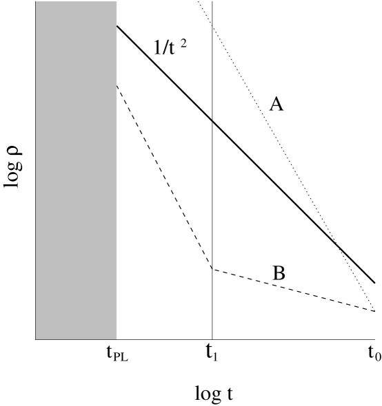
Figure 1: Scaling of the energy density in dangerous modes before and after compactification. Without a mass, a dangerous mode scales more rapidly than $t^{-2}$ and eventually dominates the energy density of the universe, as illustrated in A. With a mass, the dangerous mode scales much more slowly than $t^{-2}$, until a time $t_{1}$ at which $m=H$, as seen in B. After this point, the mode will scale as usual. The chaos is “controlled” when the dangerous energy density cannot catch up to $1/t^{2}$ before the Planck regime is reached at $t_{PL}$.

Using this equation of state argument, we can estimate the exponential suppression of the energy density in massive fields. The basic process by which dangerous modes are suppressed, and then grow near the big crunch is illustrated in Figure 1. Although we have discussed only the scalar case above, the same $w=0$ scaling when $m/H>1$ obtains for general $p$–form fields, as discussed in Appendix 1, and so this estimate applies to those fields as well. It is important to emphasize that, while the energy density in massive modes is always growing, it grows more slowly than the $t^{-2}$ scaling required for the field to be cosmologically relevant. Therefore, if we wish to estimate the importance of a given energy component, we should consider the ratio of the energy density in the component to $t^{-2}$. This quantity, $t^{2}\rho(t)$, may be thought of as measuring the ratio of the energy density in a given component to the total density, for,

$$t^{2}\rho(t)\sim\frac{\rho(t)}{H^{2}}\sim\frac{\rho(t)}{\rho_{tot}(t)},$$ (16)

where we have used Planck units. Only when $t^{2}\rho(t)$ is increasing as $t\to 0$ can a given component grow to dominate the universe.

We begin by choosing a reference time $t_{0}$, at the beginning of the contracting phase. We consider a model where the four–dimensional effective theory begins to contract with a background equation of state $\bar{w}$, so that,

$$a(t)=(t/t_{0})^{\frac{2}{3(1+\bar{w})}},$$ (17)

where we have normalized $a=1$ when $t=t_{0}$. Combining this with (14), one finds that for massive modes,

$$t^{2}\rho(t)=\left[t^{2}\rho(t)\right]_{0}\cdot(t/t_{0})^{\frac{2\bar{w}}{1+\bar{w}}},\qquad(m/H>1),$$ (18)

where $\left[t^{2}\rho(t)\right]_{0}$ denotes $t^{2}\rho(t)$ evaluated at $t_{0}$. This equation is valid up until $m/H\sim 1$, when the mass terms are becoming irrelevant. Denoting by $t_{1}$ the time at which $m=H$, one finds,

$$\frac{t_{1}}{t_{0}}=R_{c}H_{0},$$ (19)

where we have taken $m=1/R_{c}$. We then have,

$$\left[t^{2}\rho(t)\right]_{1}=\left[t^{2}\rho(t)\right]_{0}\cdot(R_{c}H_{0})^{\frac{2\bar{w}}{1+\bar{w}}},\qquad(m/H\sim 1).$$ (20)

This equation shows the suppression in the fractional energy density in massive modes during the period in which $m/H>1$. The suppression is controlled by the ratio of the compactification length scale $R_{c}$ to the Hubble horizon $L_{H}=1/H_{0}$ at the beginning of the contracting phase.

As we approach the big crunch, we have $m/H<1$, and the dangerous modes can grow as usual. We parameterize this growth by an exponent $\delta$, so that,

$$t^{2}\rho(t)=(t/t_{1})^{-\delta}\left[t^{2}\rho(t)\right]_{1},\qquad(m/H<1).$$ (21)

when $\delta>0$, a mode will grow and eventually dominate the energy density of the universe. One can see by comparing (21) to our discussion in Section II that $\delta$ is merely twice the amount by which a given mode violates the stability conditions. Typically, $\delta$ will be of order one. Now we define a time $t_{eq}$, at which the dangerous modes have grown sufficiently so that the fractional energy density in dangerous modes is equal to that at the beginning of the contracting phase, or,

$$\left[t^{2}\rho(t)\right]_{eq}=\left[t^{2}\rho(t)\right]_{0}.$$ (22)

Using (20) and (21), we find,

$$t_{eq}=t_{0}(R_{c}H_{0})^{1+\frac{2\bar{w}}{\delta(1+\bar{w})}}$$ (23)

Finally, we define a time $t_{dom}$, at which the dangerous modes formally dominate the universe, corresponding to $t^{2}\rho(t)\sim 1$. Then one finds,

$$t_{dom}=t_{eq}\left(\left[t^{2}\rho(t)\right]_{0}\right)^{1/\delta}.$$ (24)

Chaos is controlled provided that the dangerous modes do not dominate before a Planck time from the big crunch, corresponding to $t_{dom}<t_{PL}$.

Having established the formulae we will need for our estimate, we may now insert reasonable values for our variables. Let us assume the contraction phase begins when the Hubble parameter is of order the present value $H_{0}$ (as occurs in ekpyrotic and cyclic models). Then, $1/H_{0}\sim 10^{61}$ $L_{PL}$. As a first example, we assume that $\bar{w}=1$ during the contraction as is characteristic of compactifications of Kasner universes. A typical value for $\delta$ that arises from working with the $p$–form spectrum of string models and gravity is $\delta=2$, although the precise value of $\delta$ will of course depend on the specific model under consideration. If we take $R_{c}\sim 10\cdot L_{PL}$, as an example, then we find the suppression factor (20) at $H\sim m$ to be,

$$(R_{c}H_{0})^{\frac{2\bar{w}}{1+\bar{w}}}\sim 10^{-60}.$$ (25)

The dangerous modes grow to have the same fractional energy density as they had at the beginning of the contracting phase at the time,

$$t_{eq}\sim 10^{-29}\;t_{PL}.$$ (26)

Thus, the dangerous modes cannot grow to be even as relevant as at the beginning of cosmic contraction, until the universe is well within the quantum regime. We would need to approach even closer to the big crunch for these modes to dominate the universe, but at this point we no longer expect our classical equations to be valid.

As another example, we consider a case with large compact dimensions, where $m$ is of order the weak scale, $10^{-16}$ $M_{PL}$, which corresponds to taking $R_{c}\sim 10^{16}$ $L_{PL}$. Now we find that the suppression when the Hubble radius equals the compactification scale is,

$$(R_{c}H_{0})^{\frac{2\bar{w}}{1+\bar{w}}}\sim 10^{-45},$$ (27)

and,

$$t_{eq}=10^{-6}\;t_{PL}.$$ (28)

Again, we will be well within the quantum gravity regime before the dangerous modes can potentially dominate. If $\bar{w}\gg 1$ during the contraction phase, as occurs in ekpyrotic and cyclic models, the dangerous modes are suppressed by a much greater factor than in these examples, as is evident from the expressions above.

As a final relevant issue, note that we have taken the mass $m$ of the dangerous modes to be constant in time. Generally we expect that the mass $m$ of a given field will be time dependent. This occurs since the field’s mass is determined by the compactification manifold $\mathcal{M}$, and $\mathcal{M}$ will be evolving with time during cosmic contraction. Let us say that the mass $m(t)$ evolves as,

$$m(t)=m_{0}\left(\frac{t}{t_{0}}\right)^{b},$$ (29)

during the contracting phase, where for simplicity we take $\bar{w}=1$. Then, because the energy density will go like $\rho\sim m/a^{3}$, we find that

$$t^{2}\rho=\left[t^{2}\rho\right]_{0}\left(\frac{t}{t_{0}}\right)^{1+b}$$ (30)

However, the time $t_{1}$ at which $m/H\sim 1$ is now,

$$t_{1}^{1+b}=\frac{t_{0}^{b}}{m_{0}},$$ (31)

and therefore the suppression when $m/H\sim 1$ is,

$$\frac{\left[t^{2}\rho\right]_{1}}{\left[t^{2}\rho\right]_{0}}=(H_{0}/m_{0})\sim(H_{0}R_{c,0}),$$ (32)

where $R_{c,0}$ is the characteristic length of $\mathcal{M}$ when $t=t_{0}$. This is precisely the factor found in the case where $m$ is constant in time (20). The difference is that the time $t_{1}$, at which $m/H\sim 1$, shifts. This shift compensates for the different growth rate of $\rho$, with the net result that the suppression factor remains the same.

From the equations above, it is clear that there is a potential problem if $b<-1$, which would lead to $t^{2}\rho$ increasing during the contracting phase. However, our assumption that the universe is of Kasner type excludes this possibility. Field masses $m$ are related to the compactification length scale $R_{c}$ by $m\sim 1/R_{c}$. In a Kasner universe, we expect that $R_{c}\sim t^{p}$, with $p$ a Kasner exponent, or average of several Kasner exponents. However, the Kasner conditions (3) or (7) imply that $p\leq 1$, and thus $m$ must vary more slowly than $1/t$. This implies that $b\geq-1$, and so the suppression operates as before.

III.2 The $p$–form spectrum

Having established that the massless modes are the only relevant modes near the big crunch, we now describe how these massless modes are determined in terms of the compactification manifold $\mathcal{M}$. The story is familiar from the study of higher–dimensional models of particle physics Pol98 ; GSW87 ; Duf86 although we discuss some special features of the time dependent situation which must be taken into account. An useful feature of the $p$–form mass spectrum is that the existence of massless modes is determined entirely by the topology of $\mathcal{M}$, and not by its metric. This simplifies the task of finding manifolds $\mathcal{M}$ that lead to controlled chaos, since we need only specify their topological properties.

III.2.1 Time independent compactification

First, we will review the situation for the time independent case. For clarity, we will neglect here the exponential coupling to the dilaton field, which amounts to an overall multiplication by $e^{\lambda\phi}$ of the Lagrangian density. The coupling is fully accounted for in the analysis given in Appendix 1. The action for a $p$–form gauge potential $A_{p}$ in $4+n$ dimensions is,

$$S=-\frac{1}{(p+1)!}\int\mbox{d}A_{p}\cdot\mbox{d}A_{p}\,\sqrt{-G}\;d^{4+n}x,$$ (33)

where $A_{p}$ can depend on all coordinates, and has indices along both $\mathbf{R}^{1,3}$ and $\mathcal{M}$,

$$A_{p}=\left[A_{p}(x^{\mu},x^{m})\right]_{\alpha_{1}\alpha_{2}\dots\alpha_{r}a_{1}a_{2}\dots a_{p-r}}.$$ (34)

The conventional compactification analysis begins with an expansion of the $p$–form $A_{p}$ as,

$$A_{p}=\sum_{r+s=p}\sum_{i}\alpha^{(i)}_{r}\wedge\beta^{(i)}_{s}$$ (35)

using a basis of $s$–forms $\beta^{(i)}_{s}$, with indices and coordinate dependence only along $\mathcal{M}$,

$$\beta^{(i)}_{s}=\left[\beta^{(i)}_{s}(x^{m})\right]_{a_{1}a_{2}\dots a_{s}}.$$ (36)

The abstract index $i$ labels the $s$–form under consideration, and when $\mathcal{M}$ is compact it takes discrete values, infinite in number. The “coefficients” in this expansion are $r$–forms $\alpha^{(i)}_{r}$, that depend on the noncompact coordinates on $\mathbf{R}^{1,3}$, and have indices along $\mathbf{R}^{1,3}$ only,

$$\alpha^{(i)}_{r}=\left[\alpha^{(i)}_{r}(x^{\mu})\right]_{\alpha_{1}\alpha_{2}\dots\alpha_{r}}.$$ (37)

It is convenient to choose the gauge $\mbox{d}^{\dagger}\beta_{s}^{(i)}=0$, and select the $\beta^{(i)}_{s}$ to be eigenfunctions of the Hodge–de Rham Laplacian $\Delta=\mbox{d}\mbox{d}^{\dagger}+\mbox{d}^{\dagger}\mbox{d}$ on $\mathcal{M}$, with eigenvalues $\lambda^{(i)}_{s}$,

$$\Delta\beta^{(i)}_{s}=\lambda^{(i)}_{s}\beta^{(i)}_{s}.$$ (38)

The $\beta^{(i)}_{s}$ are normalized so that,

$$\int_{\mathcal{M}}\beta^{(i)}_{s}\cdot\beta^{(j)}_{s}\,\sqrt{-f}\;d^{n}x=\delta_{ij}.$$ (39)

Substituting the expansion (35) into the original action (33) results in,

$$\ S=-\sum_{i,s}\frac{1}{(r+1)!}\int\left(\mbox{d}\alpha^{(i)}_{r}\cdot\mbox{d}\alpha^{(i)}_{r}+\lambda^{(i)}_{s}\alpha^{(i)}_{r}\cdot\alpha^{(i)}_{r}\right)\,\sqrt{-h}\;d^{4}x,$$ (40)

where we have rescaled the $\alpha^{(i)}_{r}$ by a constant in order to canonically normalize the kinetic terms. This demonstrates that a single $p$–form in $4+n$ dimensions yields many $r$–forms $\alpha^{(i)}_{r}$ after compactification, whose masses $m^{(i)}_{r}$ are related to the eigenvalues $\lambda^{(i)}_{s}$ by $\left(m^{(i)}_{r}\right)^{2}=\lambda^{(i)}_{s}$. These are the “Kaluza–Klein” modes. The operator $\Delta$ has a positive semi–definite spectrum on manifolds which, like $\mathcal{M}$, have a Euclidean metric. Therefore the effective masses are all real.

The $(p-s)$–forms with zero effective mass are determined entirely by the topology of $\mathcal{M}$, and not by its metric structure. As discussed above, massless $(p-s)$–forms arise from $s$–forms $\beta_{s}$ satisfying $\Delta\beta^{(i)}_{s}=0$, conventionally termed “harmonic” forms. Hodge’s theorem Nak90 ; EGH80 states that the number of harmonic $s$–forms is equal to the dimension of $\mathcal{H}^{s}\left(\mathcal{M}\right)$, the $s^{th}$ de Rham cohomology class of $\mathcal{M}$. The dimension $\dim\mathcal{H}^{s}\left(\mathcal{M}\right)$ is also known as the $s^{th}$ Betti number of $\mathcal{M}$, conventionally denoted $b_{s}(\mathcal{M})$. This is a topological invariant, which does not change under smooth deformations of $\mathcal{M}$ and its associated metric structure. The Poincaré duality theorem Mas91 ; Mad97 gives a simple geometric interpretation of these cohomology classes; the quantity $\dim\mathcal{H}^{s}\left(\mathcal{M}\right)$ counts the number of $s$–dimensional submanifolds that can “wrap” $\mathcal{M}$, and cannot be smoothly contracted to zero. In this counting, two submanifolds are considered equivalent if one can be smoothly deformed into the other. Thus, for every inequivalent noncontractible submanifold of $\mathcal{M}$ with dimension $s$, a $p$–form gives rise to a massless $(p-s)$–form field after compactification.

III.2.2 Time dependent compactification

The case where the compactification manifold $\mathcal{M}$ changes with time introduces new features, but in the end does not substantially modify the conclusions reached above. The main difference is that it is no longer possible to assume that the eigenbasis of forms $\beta^{(i)}_{s}$ defined by (38) depends only on the compact coordinates $x^{m}$. In particular, the forms will depend on time. This introduces additional cross terms which must be taken into account. Below, we will neglect the variation of $\mathcal{M}$ along directions $x^{M}$ other than time. We denote by $\mbox{d}|_{\mathcal{M}}$ the exterior derivative tangent to the manifold $\mathcal{M}$. Thus,

$$\mbox{d}\beta^{(j)}_{s}=\mbox{d}|_{\mathcal{M}}\beta^{(i)}_{s}+\mbox{d}t\wedge\dot{\beta}^{(i)}_{s}.$$ (41)

We may now use our freedom to choose the basis modes $\beta^{(i)}_{s}$, and define the modes $\beta^{(i)}_{s}(t)$ with $\lambda^{(i)}_{s}(t)>0$ to be the instantaneous eigenforms of the Hodge–de Rham operator, restricted to act on $\mathcal{M}$ only,

$$\Delta|_{\mathcal{M}}\beta^{(i)}_{s}(t)=\lambda^{(i)}_{s}(t)\beta^{(i)}_{s}(t).$$ (42)

We find it convenient to relax the requirement that the zero modes $\beta^{(i)}_{s}(t)$ with $\lambda^{(i)}_{s}=0$ be eigenforms of the Hodge–de Rham Laplacian. Instead, we will merely require that they be representatives of the de Rham cohomology of $\mathcal{M}$. Inspection of the reduced action shows that this condition is sufficient to guarantee that the zero modes still result in massless form fields. Furthermore, we adopt the normalization convention,

$$\int_{\mathcal{M}}\beta^{(i)}_{s}\cdot\beta^{(j)}_{s}\,\sqrt{-f}\;d^{n}x=\delta_{ij}\int\,\sqrt{-f}\;d^{n}x.$$ (43)

This differs from the usual normalization convention (39) by only a multiplicative constant in the static case. It has the advantage of not introducing any spurious time dependence of the $\beta^{(i)}_{s}$ from the changing volume of $\mathcal{M}$. Maintaining this normalization condition requires,

$$\int_{\mathcal{M}}\dot{\beta}^{(i)}_{s}\cdot\beta^{(j)}_{s}\,\sqrt{-f}\;d^{n}x=0.$$ (44)

With these conventions and definitions, we find that the $p$–form action (33) splits into two parts, $S_{1}$ and $S_{2}$, with

$$S_{1}=-\sum_{s,i}\frac{1}{(r+1)!}\int\mbox{d}\alpha^{(i)}_{r}\cdot\mbox{d}\alpha^{(i)}_{r}+\lambda^{(i)}_{s}(t)\alpha^{(i)}_{r}\cdot\alpha^{(i)}_{r}\,\sqrt{-G}\;d^{4+n}x$$ (45)

and,

$$S_{2}=-\sum_{s,i}\frac{2}{(r+1)!}\int(\alpha^{(i)}_{r}\wedge{\dot{\beta}}^{(i)}_{s})\cdot({\dot{\alpha}}{(i)}_{r}\wedge\beta^{(i)}_{s})+(\alpha^{(i)}_{r}\cdot\alpha^{(i)}_{r})({\dot{\beta}}^{(i)}_{s}\cdot{\dot{\beta}}^{(i)}_{s})\,\sqrt{-G}\;d^{4+n}x,$$ (46)

where terms that are identically zero due to mismatched indices are not included. Again, we have rescaled the $\alpha^{(i)}_{r}$ to obtain canonically normalized kinetic terms. The terms in $S_{2}$ threaten to substantially modify the action in the time dependent case. However, these terms vanish or are negligible. The first term is zero due to our normalization convention (43) and its consequence (44). The second term is a contribution to the effective mass of $\alpha^{(i)}_{r}$. For the $\lambda^{(i)}_{s}=0$ modes, the representatives $\beta_{s}^{(i)}$ of the de Rham cohomology are time–independent, and so the $\dot{\beta}^{2}$ terms vanish. When $\lambda^{(i)}_{s}>0$, the additional contribution to the effective mass will be positive, but since these modes are already massive it will not change the qualitative features of their behavior. Thus, time dependent compactifications do not substantially modify the $p$–form spectrum; massless modes are still given by the de Rham cohomology of $\mathcal{M}$.

III.3 The gravitational spectrum

A key property of Kaluza–Klein reduction is that degrees of freedom in the full metric $G_{MN}$ appear in lower dimensions as metric, vector, and scalar degrees of freedom. As in the $p$–form compactification discussed above, the masses of these fields depend on the properties of the compactification manifold $\mathcal{M}$. In contrast to the $p$–form case, the masses are not determined by the cohomology of $\mathcal{M}$, but by the existence of Killing fields on $\mathcal{M}$. The properties of Kaluza–Klein reduction, along with our discussion of chaos in Section II, provide some useful simplifications. Since some of the metric degrees of freedom in the higher dimensional theory appear as zero– and one–forms, chaos arising from these degrees of freedom can be suppressed if they acquire a mass, just as in the conventional $p$–form case.

As an explicit example of the reduction process, and of how chaos in higher and lower dimensions are related, we consider below the simple case with a single extra dimension Bel73 . The Kaluza–Klein reduction begins with a reparameterization of the metric,

$$G_{MN}=\begin{pmatrix}e^{-q\phi}g_{\mu\nu}+e^{2q\phi}A_{\mu}A_{\nu}&e^{2q\phi}A_{\nu}\\ e^{2q\phi}A_{\mu}&e^{2q\phi}\end{pmatrix},$$ (47)

where we assume that $A_{\mu}$ and $\phi$ are independent of the fifth dimension. We substitute this metric into the Einstein–Hilbert action and integrate over the fifth dimension. The coefficient $q=\sqrt{2/3}$ is chosen so that the scalar field $\phi$ has a canonically normalized kinetic term in the resulting action,

$$S=\int R(g)-(\partial\phi)^{2}-\frac{1}{4}e^{\sqrt{6}\phi}F_{\mu\nu}F^{\mu\nu}\,\sqrt{-g}\;d^{4}x,$$ (48)

with $F_{\mu\nu}=\partial_{\mu}A_{\nu}-\partial_{\nu}A_{\mu}$. This describes Einstein gravity coupled to a scalar field $\phi$, and a vector field with $\phi$–dependent coupling. It can be seen that all of the five–dimensional metric degrees of freedom in (47) are reproduced in this four–dimensional action. Furthermore, the vector term in the action possesses an exponential coupling to $\phi$, of the type introduced in (1). Our starting point, the five dimensional pure gravity theory, is chaotic since the gravitational stability conditions cannot be satisfied for any choice of the Kasner exponents. After reduction, chaos also inevitably arises since the gravitational and one–form stability conditions cannot be satisfied simultaneously. Thus violations of the gravitational stability conditions in five dimensions can appear as violations of the $p$–form stability conditions in four dimensions. As we will discuss in more detail below, the preservation of chaos is not a generic feature of Kaluza–Klein reduction in dimensions greater than one.

The example above is limited to a single extra dimension, and neglects metric modes that depend on the fifth coordinate. Below, we consider the general case, and calculate the effective masses of all Kaluza–Klein vector fields with an arbitrary number of extra dimensions. We will find that these masses are zero only when $\mathcal{M}$ possesses Killing vectors. This calculation parallels standard treatments of Kaluza–Klein reduction Duf86 , but in these treatments the fact that $\mathcal{M}$ may not possess isometries is often not emphasized. For $n>1$ extra dimensions, we will generalize the decomposition (47) using the vielbein formalism. We begin by defining one form fields $e^{A}={e_{M}}^{A}{\mbox{d}x}^{M}$ so that,

$$ds^{2}={e}^{A}{e}^{B}\eta_{AB},$$ (49)

with $\eta_{AB}$ the $(4+n)$–dimensional Minkowski metric. The ${e_{M}}^{A}$ are chosen so that,

$$h_{\mu\nu} ={e_{\mu}}^{\alpha}{e_{\nu}}^{\beta}\eta_{\alpha\beta},$$ (50a)

$$f_{mn} ={e_{m}}^{a}{e_{n}}^{b}\delta_{ab},$$ (50b)

$${e_{\mu}}^{a} =K^{aj}(x^{m})A^{j}_{\mu}(x^{\mu}),$$ (50c)

$${e_{m}}^{\alpha} =0,$$ (50d)

where $\delta_{ab}$ the Euclidean flat space metric. The $K^{aj}$ are a basis for vector fields on $\mathcal{M}$, indexed by $j$, that depend only on the compact coordinates $x^{m}$. The coefficients in this expansion are the $A^{j}_{\mu}$, which depend only the noncompact coordinates $x^{\mu}$. The $A^{j}_{\mu}$, known as Kaluza–Klein vectors, will emerge after compactification as vector fields on the noncompact space $\mathbf{R}^{1,3}$. The commutators of the $K^{aj}$ define a set of structure constants ${f^{jk}}_{l}$,

$$[K^{j},K^{k}]={f^{jk}}_{l}K^{l}.$$ (51)

The calculation is most conveniently carried out using an orthonormal basis $\{{\hat{e}}^{a},{\hat{e}}^{\alpha}\}$ given by,

$${\hat{e}}^{\alpha}=e^{\alpha}\qquad{\hat{e}}^{a}=e^{a}-K^{aj}A^{j}_{\mu}{\mbox{d}x}^{\mu},$$ (52)

in which the line element assumes the simple form $ds^{2}={\hat{e}}^{\alpha}{\hat{e}}^{\beta}\eta_{\alpha\beta}+{\hat{e}}^{a}{\hat{e}}^{b}\delta_{ab}$. In the event that some of the $K^{aj}$ are Killing fields on $\mathcal{M}$, then the lower dimensional theory will possess a gauge symmetry. The Killing fields are generators of the isometry group of $\mathcal{M}$, and this isometry group reemerges as the gauge group in the lower dimensional theory. This motivates the definition of a “field strength” $F^{i}_{\mu\nu}$ as,

$$F^{i}=\mbox{d}A^{i}+\frac{1}{2}f^{ijk}A^{j}\wedge A^{k}.$$ (53)

In the general case, the Killing fields alone do not provide a full basis for vector fields on $\mathcal{M}$. Thus, in addition to the massless modes (if any) of the gauge theory, there will also be an infinite set of massive gauge fields in the lower dimensional theory.

In order to derive the mass spectrum in the lower dimension explicitly, we may use the vielbeins to decompose the gravitational action in $4+n$ dimensions. The spin connections are,

$${\hat{\omega}}_{ab} =\omega_{ab}-\frac{1}{2}(\nabla_{b}K_{a}^{j}-\nabla_{a}K_{b}^{j})A^{j}_{\beta}e^{\beta},$$ (54a)

$${\hat{\omega}}_{a\beta} =\frac{1}{2}K_{a}^{j}F^{j}_{\alpha\beta}e^{\alpha}+\nabla_{(b}K_{a)}^{j}A^{j}_{\beta}{\hat{e}}^{\beta},$$ (54b)

$${\hat{\omega}}_{\alpha\beta} =\omega_{\alpha\beta}+\frac{1}{2}K_{b}^{j}F^{j}_{\alpha\beta}{\hat{e}}^{b},$$ (54c)

where $\omega_{ab}$ and $\omega_{\alpha\beta}$ are the spin connections defined by the metrics $f_{mn}$ on $\mathcal{M}$, and $h_{\mu\nu}$ on $\mathbf{R}^{1,3}$, respectively. Using these spin connections to compute the Ricci scalar, one obtains,

$$R(G)=R(h)+R(f)-\frac{1}{4}K^{j}_{a}K^{ka}F^{j}_{\mu\nu}F^{k\mu\nu}-2\nabla_{(c}K^{j}_{d)}\nabla^{(c}K^{kd)}A^{j\mu}A^{k}_{\mu}.$$ (55)

We see that a mass term for the $A^{j}$ has appeared. Upon integrating over the compact coordinates, one arrives at the Jordan frame action,

$$S=\int\left(W(f)R(h)-S(f)-\frac{1}{4}\alpha_{jk}F^{j}_{\mu\nu}F^{k\mu\nu}-\beta_{jk}A^{j\mu}A^{k}_{\mu}\right)\;\sqrt{h}\,d^{4}x.$$ (56)

where,

$$W(f) =\int_{\mathcal{M}}\;\sqrt{f}\,d^{n}x$$ (57a)

$$S(f) =-\int_{\mathcal{M}}R(f)\;\sqrt{f}\,d^{n}x$$ (57b)

$$\alpha_{jk} =\int_{\mathcal{M}}K_{ja}K_{k}^{a}\;\sqrt{f}\,d^{n}x$$ (57c)

$$\beta_{jk} =2\int_{\mathcal{M}}\nabla_{(c}K_{jd)}\nabla^{(c}K_{k}^{d)}\;\sqrt{f}\,d^{n}x.$$ (57d)

The $W(f)$ factor may be removed by a rescaling of the metric $h_{\mu\nu}$, putting the action in the Einstein frame form. The $S(f)$ term will yield a system of scalar fields, of which $\phi$ in our five dimensional reduction (48) is an example. Applying the Gram–Schmidt orthonormalization process to the $K^{j}$, one can reduce $\alpha_{jk}=\delta_{jk}$, giving the vectors a canonical kinetic term. Thus, we see Kaluza–Klein reduction of pure gravity results in a theory with scalars and vector fields, generalizing the $n=1$ result discussed above.

Of crucial importance to the present work is that massless Kaluza–Klein vectors are in one–to–one correspondence with Killing fields on $\mathcal{M}$, or equivalently the zero eigenvalues of $\beta_{jk}$. This follows from the fact that $\beta_{jk}$ functions as a mass matrix for the Kaluza–Klein vector fields. Since $\beta_{jk}$ is symmetric, we are guaranteed that $m^{2}$ will be real for all modes. In our discussion of $p$–form fields, we were able to apply powerful results regarding the Hodge–de Rham operator $\Delta$ that guaranteed that $m^{2}\geq 0$, regardless of the topology and metric structure of $\mathcal{M}$. In the present situation, we have no guarantee that the masses of Kaluza–Klein vectors will satisfy $m^{2}\geq 0$, or equivalently that the eigenvalues of the mass matrix are nonnegative.

In this work we will assume that all eigenvalues of the mass matrix are nonnegative, so that $m^{2}\geq 0$ for all Kaluza–Klein vectors. In the general case, it is necessary to compute $\alpha_{jk}$ and $\beta_{jk}$ for each manifold of interest, and then check that this assumption holds on a case–by–case basis. A simple example is provided by the $n$–torus $\mathbf{T}^{n}$. Realizing the torus as $\mathbf{R}^{n}/\mathbb{Z}^{n}$, with coordinates $(\theta_{1}\dots\theta_{n})$ ranging on $(0,2\pi)$, a convenient basis for vector fields on $\mathbf{T}^{n}$ is provided by,

$$K^{(a,n)}=\frac{\sqrt{2}\hat{\theta}^{a}}{(2\pi)^{n/2}}\times\begin{cases}\cos n\theta,&\qquad\mbox{for }n\geq 0,\\ \sin n\theta,&\qquad\mbox{for }n<0\end{cases}$$ (58)

where $n\in\mathbb{Z}$, the $\hat{\theta}^{a}$ are unit vectors associated to each coordinate, and $(a,n)$ label each basis field, replacing the abstract indices used above. Substituting this into (57) we find,

$$\alpha_{(a,n)(b,m)} =\delta_{ab}\delta_{nm},$$ (59a)

$$\beta_{(a,n)(b,m)} =2n^{2}\delta_{ab}\delta_{nm}.$$ (59b)

The Kaluza–Klein vector fields are therefore canonically normalized, with masses $\sqrt{2}n$ for $n=0,1,2\dots$, showing our assumption is valid in this case. More sophisticated examples may be found in the literature Duf86 . As we will explain in more detail below, the $m^{2}\geq 0$ assumption will enable us to treat $p$–forms and Kaluza–Klein vectors on the same footing.

IV Selection Rules for the Stability Conditions

With the tools developed in the previous sections, we are now prepared to discuss conditions on $\mathcal{M}$ that result in controlled chaos. We will show that the gravitational, electric and magnetic stability conditions, introduced in Section II, are modified by compactification. Not all of the stability conditions remain relevant, and only a subset need be satisfied to ensure that chaos is controlled. This subset is defined by the “selection rules” that are the focus of this section. The selection rules that determine when a stability condition remains relevant are given for matter fields in Section IV.1, and for gravitational modes in IV.2. The selection rules, in turn, are determined by the de Rham cohomology (in the $p$–form case) and existence of Killing vectors (in gravitational case) of the compactification manifold $\mathcal{M}$. Here, we focus on discussing the origin of the selection rules. Once established, we will use them to find compactifications that control chaos in Section V.

IV.1 The $p$–form selection rules

The discussion in Section III enables us to define selection rules for the electric and magnetic stability conditions. Each component of the $p$–form field results in an electric or magnetic stability condition, which expresses whether the energy density in that component scales rapidly enough to dominate the energy density of the universe and cause chaos. If this component gains a mass by compactification, then we have shown that it scales too slowly to be cosmologically relevant, and therefore we should ignore the corresponding stability condition. Thus we should ignore all electric and magnetic stability conditions involving indices that do not correspond to massless $p$–form modes. This results in the following selection rule,

The $p$–form Selection Rule: When $\dim\mathcal{H}^{s}\left(\mathcal{M}\right)=0$ for some $s$, ignore the subset of $p$–form stability conditions,

$$\sum_{p}p_{j}-\frac{1}{2}\lambda p_{\phi} >0\qquad\mbox{(electric)},$$ (60a)

$$\sum_{p+1}p_{j}-\frac{1}{2}\lambda p_{\phi} <1\qquad\mbox{(magnetic)},$$ (60b)

with $s$ Kasner exponents along the compact space $\mathcal{M}$. Retain only those stability conditions with $s$ exponents along $\mathcal{M}$ and $\dim\mathcal{H}^{s}\left(\mathcal{M}\right)\neq 0$.

In this section, we will use the results of previous sections to prove this rule, and give some simple examples of its use.

This rule arises from considering the $p$–form modes that give rise to massless fields after compactification. A $p$–form $A_{p}$ gives rise to a massless $r$–form $\alpha_{r}$ if and only if $A_{p}$ is of the form,

$$A_{p}=\alpha_{r}\wedge\beta_{s}$$ (61)

where $\beta_{s}\in\mathcal{H}^{s}\left(\mathcal{M}\right)$, and $r+s=p$. Since $\mbox{d}\beta_{s}=0$, this gauge potential results in the field strength,

$$F_{p+1}=(\mbox{d}\alpha)_{r+1}\wedge\beta_{s}.$$ (62)

When the energy density of this field is calculated, one finds a stability condition involving exactly $s$ Kasner exponents along $\mathcal{M}$, and the remainder along $\mathbf{R}^{1,3}$. Since only stability conditions of this type correspond to massless modes, they are the only ones that should be retained.

The case (62) deals only with field strengths having at least one index along the noncompact space $\mathbf{R}^{1,3}$. In fact, the same selection rule applies when all indices of the field strength are along $\mathcal{M}$. In this case, the field strength must satisfy the Bianchi identity and the Gauss law,

$$\mbox{d}F_{p+1}=0,\qquad\mbox{d}^{\dagger}F_{p+1}=0.$$ (63)

Field strengths of this type are commonly termed “nonzero modes” GSW87 . The conditions (63) imply that $F_{p+1}$ is harmonic, and by Hodge’s theorem the number of such forms is given by $\dim\mathcal{H}^{p+1}\left(\mathcal{M}\right)$. When $\dim\mathcal{H}^{p+1}\left(\mathcal{M}\right)$ vanishes, we cannot have a $p$–form field strength with all indices along $\mathcal{M}$, and we should therefore delete the corresponding stability condition, with $(p+1)$ Kasner exponents along $\mathcal{M}$. Thus this case falls under the $p$–form selection rule as well.

The selection rule may be illustrated by comparing compactification on a sphere $\mathbf{S}^{n}$ and a torus $\mathbf{T}^{n}$ . These manifolds encompass the best and worst case scenarios for controlling chaos through compactification. The sphere has the minimum number of massless modes for any orientable compact manifold, while the torus has massless modes for every dimension and involving every combination of indices on $\mathcal{M}$. Therefore compactification on $\mathbf{T}^{n}$ and $\mathbf{S}^{n}$ will have very different influences on chaotic behavior.

Compactification on $\mathbf{T}^{n}$ does not modify any of the $p$–form stability conditions. The cohomology classes of the torus are,

$$\dim\mathcal{H}^{r}\left(\mathbf{T}^{n}\right)=\frac{n!}{r!(n-r)!},\qquad 0\leq r\leq n.$$ (64)

If we realize the torus as $\mathbf{R}^{n}/\mathbb{Z}^{n}$, with coordinates $\theta_{1},\dots\theta_{n}$, then we may choose the following set of generators for the $r^{th}$ de Rham class,

$$\omega_{r}=\mbox{d}\theta_{j_{1}}\wedge\mbox{d}\theta_{j_{2}}\wedge\dots\wedge\mbox{d}\theta_{j_{r}},$$ (65)

where $\{j_{r}\}$ are any set of distinct indices on $\mathbf{T}^{n}$. Therefore, massless modes exist for $p$–form fields with any combination of indices along the $\mathbf{T}^{n}$. Any $p$–form stability condition that appears in the noncompactified theory will remain in the compactified theory.

By contrast, compactification on a sphere $\mathbf{S}^{n}$, with $n>1$, deletes many of the stability conditions. The sphere has only two nonzero cohomology groups, each of unit dimension;

$$\dim\mathcal{H}^{r}\left(\mathbf{S}^{n}\right)=\begin{cases}1,\qquad&\text{for}\quad r=0\quad\text{and}\quad r=n\\ 0,\qquad&\text{otherwise}.\end{cases}$$ (66)

The class $\mathcal{H}^{0}\left(\mathbf{S}^{n}\right)$ is generated by the constant scalar function on $\mathbf{S}^{n}$, while the class $\mathcal{H}^{n}\left(\mathbf{S}^{n}\right)$ is generated by the volume form,

$$\omega_{n}=\sqrt{g}\,\mbox{d}\theta_{1}\wedge\mbox{d}\theta_{2}\wedge\dots\wedge\mbox{d}\theta_{n},$$ (67)

where $g_{mn}$ is the metric, $g=\det g_{mn}$, and $\theta_{j}$ the coordinates on the sphere. Massless modes therefore contain either no indices along the $\mathbf{S}^{n}$, or all indices at once. This implies that the only surviving stability conditions are those with either no internal Kasner exponents, or all internal Kasner exponents together. In the case where $n>p$, none of the internal Kasner exponents appear at all, and only those stability conditions involving Kasner exponents on $\mathbf{R}^{1,3}$ survive.

Our statement of the selection rule is the strongest possible in the generic case, and fortunately also the most conservative in terms of deleting the minimum number of stability conditions. Manifolds with a specific relationship between the frames $\sigma^{a}$ appearing in (2) and the cohomology representatives of $\mathcal{M}$ may require that we delete additional $p$–form stability conditions. For example, consider the case in which $\mathcal{M}$ factors as $\mathcal{M}=\mathcal{M}_{1}\times\mathcal{M}_{2}$, both topologically and metrically. A straightforward application of the selection rules results in retaining all stability conditions with $s$ indices along $\mathcal{M}$ whenever $\dim\mathcal{H}^{s}\left(\mathcal{M}\right)\neq 0$. These stability conditions correspond to $p$–form modes with $s_{1}$ indices along $\mathcal{M}_{1}$ and $s_{2}$ indices along $\mathcal{M}_{2}$, with $s_{1}+s_{2}=s$. However, in general a massless mode will not exist for every choice of $s_{1}$ and $s_{2}$, and therefore we may be able to delete additional stability conditions. We should only retain the even smaller subset of stability conditions with $s_{1}$ Kasner indices along $\mathcal{M}_{1}$ and $s_{2}$ indices along $\mathcal{M}_{2}$ when $\dim\mathcal{H}^{s_{1}}\left(\mathcal{M}_{1}\right)\neq 0$ and $\dim\mathcal{H}^{s_{2}}\left(\mathcal{M}_{2}\right)\neq 0$. Generally, however, we do not expect any special relationship between the $\sigma_{j}$ and the cohomology classes. In this example, we have imposed the condition by hand that the $\sigma_{j}$ point only along exactly one of $\mathcal{M}_{1}$ or $\mathcal{M}_{2}$. Examples such as this one must be considered on a case–by–case basis, and lie beyond the scope of our selection rule.

IV.2 The gravitational selection rules

The selection rules for the gravitational stability conditions arise in a manner similar to those for the $p$–form modes. We identify the degree of freedom corresponding to each stability condition, and then ignore the stability condition if the degree of freedom gains a mass through compactification. Unlike the $p$–form case, in general one must also check that the masses gained in this way satisfy $m^{2}\geq 0$, as discussed at the end of Section III.3. In this way, we arrive at a selection rule for the gravitational stability conditions,

The Gravitational Selection Rule: When $\mathcal{M}$ possesses no Killing vectors, retain only the subset of gravitational stability conditions,

$$p_{i}+p_{j}-p_{k}<1,\qquad\mbox{all triples}\quad i,j,k,$$ (68)

with all three Kasner exponents along $\mathbf{R}^{1,3}$, or all three along $\mathcal{M}$, and ignore stability conditions with a mixture of exponents along both $\mathbf{R}^{1,3}$ and $\mathcal{M}$.

In proceeding, we are guided by the Kaluza–Klein reduced Jordan frame action (56). Clearly, gravitational stability conditions involving three Kasner exponents along the $\mathbf{R}^{1,3}$ should be retained, as the corresponding modes do not gain a mass from compactification. These represent the metric degrees of freedom in the lower dimensional theory. Stability conditions involving three Kasner exponents along the compact direction should also be retained. Physically, these correspond to metric degrees of freedom on compact space $\mathcal{M}$. While these appear as scalar fields in the lower dimensional theory, they can result in a subtle form of chaos. Violations of these stability conditions appears as a chaotic system of interacting scalars in the lower dimensional theory. Thus, to ensure that all degrees of freedom are evolving smoothly to the big crunch, we should retain these stability conditions.

Compactification can delete the “mixed” stability conditions, those with Kasner exponents along both $\mathbf{R}^{1,3}$ and $\mathcal{M}$. These appear as the kinetic and mass terms for the Kaluza–Klein vectors in (56). When the compact space $\mathcal{M}$ possesses no Killing vectors, then these vector fields acquire a mass and become cosmologically irrelevant. When $\mathcal{M}$ possesses even one Killing vector, then in general none of the mixed stability conditions can be discarded. This is because a single Killing field will generally involve all indices along $\mathcal{M}$, and also results in a vector field with arbitrary indices on $\mathbf{R}^{1,3}$. As in the $p$–form case, there can be special cases where additional stability conditions may be deleted. However, as we are more interested in the generic case we will not discuss examples here.

V Examples

The previous sections have established that compactification allows us to ignore a number of the gravitational and $p$–form stability conditions. At this point, it is natural to ask if there are examples where enough stability conditions are deleted to control chaos. We show below that this is indeed the case, by giving explicit examples from both pure Einstein gravity and the low–energy bosonic sectors of string theory. We will discuss several solutions with controlled chaos in string models with $\mathcal{N}=1$ supersymmetry in ten dimensions, and will show how these solutions are interrelated by string duality relationships.

For simplicity, we focus on regions on the Kasner sphere near what we will term “doubly isotropic” solutions. These are solutions in which $a$ Kasner exponents take the value $p_{a}$, and $b$ take the value $p_{b}$, with $a+b=D-1$. In the absence of a dilaton, the Kasner conditions (3) result in a quadratic equation for $p_{a}$ and $p_{b}$, and therefore two solutions for each choice of $a$ and $b$. When a dilaton is present, then there are two one–parameter families of $p_{a}$ and $p_{b}$, which depend on the value of the dilaton “Kasner exponent” $p_{\phi}$. Only models that are isotropic in three noncompact directions are of interest cosmologically, and so we fix $a=3$. The Kaluza–Klein reduction of such models results in an isotropic universe with $p_{1}\dots p_{3}=1/3$, corresponding to a FRW universe dominated by a component with equation of state $w=1$.

It is important to emphasize that the specific examples that we will discuss are only representative points of an open region on the Kasner circle for which chaos is controlled, chosen so that the Kasner exponents assume a particularly simple, symmetric form. For a given compactification, the selection rules define a reduced set of stability conditions, which in turn define an open region of the Kasner circle for which all stability conditions are satisfied. When this open region is non–empty, then chaos is controlled. Thus, there will be choices of the Kasner exponents with controlled chaos in open neighborhoods of all of the solutions discussed herein.

V.1 Pure gravity models

The simplest case, with $n=1$ extra dimensions, is also a somewhat exceptional one. This is because there is exactly one compact one dimensional manifold, the circle $\mathbf{S}^{1}$. Regardless of the metric on the $\mathbf{S}^{1}$, it will always possess a Killing vector, and so no gravitational stability conditions can be deleted. Furthermore, $\mathcal{H}^{1}\left(\mathbf{S}^{1}\right)$ is nonzero, and so no $p$–form stability conditions are deleted. Therefore, all chaotic models remain chaotic when compactified on $\mathbf{S}^{1}$. To eliminate chaos when $n=1$, we must consider a more general class of spaces than manifolds.

For Einstein gravity without matter, a simple example that eliminates chaos when $n=1$ is given by the orbifold $\mathbf{S}^{1}/\mathbb{Z}_{2}$, previously discussed in Ref. Eri03 . If we take a coordinate $\theta$ on $\mathbf{S}^{1}$, ranging from $[-\pi,\pi]$, then the orbifold results from identifying the $\mathbf{S}^{1}$ under the reflection $\theta\to-\theta$. This takes $G_{\mu\theta}\to-G_{\mu\theta}$, and thus the Killing field is projected out, giving mass to all the Kaluza–Klein vectors. The resulting action for massless fields in four dimensions is then,

$$S=\int R(g)-(\partial\phi)^{2}\,\sqrt{-g}\;d^{4}x,$$ (69)

in comparison with the classic Kaluza–Klein result (48). Being only Einstein gravity with a scalar field, this theory is not chaotic. We will discuss compactification on this particular orbifold in more detail when we discuss string and M–theory solutions with controlled chaos.

When we have $n>1$ extra dimensions, then chaos can be eliminated by compactifying on a manifold without continuous isometries, and therefore without Killing vectors. This deletes the mixed gravitational stability conditions, as discussed in Section IV.2. The remaining stability conditions are always satisfied in the neighborhood of doubly isotropic solutions. This is subject to the assumption, discussed at the end of III.3, that the mass matrix for the Kaluza–Klein vector modes has no negative eigenvalues.

While we have seen that the masses of Kaluza–Klein vectors are determined by isometric properties of $\mathcal{M}$, there is a useful class of manifolds for which these properties are themselves determined by the topology, specifically by the de Rham cohomology. In this case, the gravitational and $p$–form selection rules are determined entirely by the cohomology of $\mathcal{M}$. These are the Einstein manifolds, for which,

$$R_{MN}=\lambda g_{MN},$$ (70)

with $\lambda$ arbitrary. When $\mathcal{M}$ is Einstein, the number of Killing vectors is given by $\dim\mathcal{H}^{1}\left(\mathcal{M}\right)$ Bes87 . Chaos will thus be controlled in a neighborhood of doubly isotropic solutions when $\dim\mathcal{H}^{1}\left(\mathcal{M}\right)=0$. There are many examples of Einstein manifolds with this property; among them are the complex projective spaces $\mathbb{C}\mbox{P}^{n}$ with the Fubini–Study metric, and the Calabi–Yau spaces.

V.2 String models

For string models with $\mathcal{N}=1$ supersymmetry in ten dimensions (Type I and heterotic), the simple class of doubly isotropic solutions is sufficient to give examples of solutions with controlled chaos. As we will discuss in more detail below, some of our solutions are related to others through standard string duality relationships. Interestingly, we find that theories with $\mathcal{N}=2$ supersymmetry (Type II) do not admit compactifications that lead to controlled chaos with doubly isotropic solutions. Unfortunately, we have found no examples where the compactification manifold could be a Calabi–Yau, although solutions with controlled chaos and Calabi–Yau compactification may exist for non–doubly isotropic choices of the Kasner exponents.

In the following, we will always give the Kasner exponents in the Einstein conformal frame. Conventionally, the bosonic sector of string theory actions is presented in the “string frame” form,

$$S_{\text{string}}=\int\left(e^{-2\Phi}\left[R(G^{(S)})+4(\partial\Phi)^{2}\right]-\sum_{j}e^{\lambda^{(S)}_{j}\Phi}F_{p_{j}+1}^{2}\right)\;\sqrt{-G^{(S)}}\,d^{10}x$$ (71)

where the $\lambda^{(S)}_{j}$ are the string frame couplings to the dilaton field, and $G^{(S)}$ the string frame metric. One arrives at the “Einstein frame” action by the transformation,

$$G_{MN}^{(E)}=e^{-\Phi/2}G_{MN}^{(S)}$$ (72)

resulting in,

$$S_{\text{Einstein}}=\int\left(R(G^{(E)})-(\partial\phi)^{2}-\sum_{j}e^{\lambda^{(E)}_{j}\phi}F_{p_{j}+1}^{2}\right)\;\sqrt{-G^{(E)}}\,d^{10}x$$ (73)

where we have defined,

$$\phi =\Phi/\sqrt{2},$$ (74a)

$$\lambda^{(E)}_{j} =\sqrt{2}\left(\lambda^{(S)}+\frac{8-2p_{j}}{4}\right),$$ (74b)

The field $\phi$, which we shall refer to as the “dilaton” below, is canonically normalized, and the couplings between the dilaton and $p$–forms have transformed. In the following, we will always use the Einstein frame couplings, and so will drop the superscript $(E)$ for clarity in notation.

A theme common to our examples is the compatibility of our results concerning controlled chaos and the duality relationships connecting various string theories. In Section V.2.1 we first examine the $\text{E}_{8}\times\text{E}_{8}$ heterotic theory in detail. Through a combination of string duality relationships and compactifications we will be able to discuss its limits in eleven, ten, five and four dimensions. In particular, the S–duality relating the $\text{E}_{8}\times\text{E}_{8}$ heterotic string and M–theory Hor95 ; Hor96 is made apparent by relating the ten dimensional heterotic solution with controlled chaos and the compactification of eleven dimensional M–theory on $\mathbf{S}^{1}/\mathbb{Z}_{2}$. We will then discuss all compactifications of doubly isotropic solutions with controlled chaos for string theories with $\mathcal{N}=1$ supersymmetry in ten dimensions. We give four representative solutions, two each for the heterotic and Type I theories. We show that these four solutions organize into two pairs of solutions, related by the S–duality connecting the heterotic SO(32) and Type I strings Pol98 .

It is important to keep in mind some features of the space of string solutions with controlled chaos. Each compactification we discuss, defined by the vanishing de Rham cohomology classes, defines an open region on the Kasner circle where chaos is controlled. Our restriction to doubly isotropic models, in turn, takes a one dimensional “slice” out of this open region. In our examples, we give a representative point from the “slice” where the Kasner exponents assume a convenient and symmetric form. Thus we have found the compactifications that admit doubly isotropic solutions, but the choices of Kasner exponents are not unique.

V.2.1 The heterotic string and M–theory

theory	spacetime	dim	$p_{1}\dots p_{3}$	$p_{4}\dots p_{9}$	$p_{10}$	$p_{\phi}$
M–theory	$\mathbf{R}^{1,3}\times\mathcal{M}\times\mathbf{S}^{1}/\mathbb{Z}_{2}$	11	-0.1206	0.0662	0.9644
het $\text{E}_{8}\times\text{E}_{8}$	$\mathbf{R}^{1,3}\times\mathcal{M}$	10	0	$1/6$		$\sqrt{5/6}$
“braneworld”	$\mathbf{R}^{1,3}\times\mathbf{S}^{1}/\mathbb{Z}_{2}$	5	0.0105		0.9686	0.2486
FRW	$\mathbf{R}^{1,3}$	4	1/3			$\sqrt{2/3}$

Table 1: The solution discussed in the text for the $\text{E}_{8}\times\text{E}_{8}$ heterotic string in various dimensions. The Kasner exponent $p_{\phi}$ is a combination of the dilaton and volume modulus for the compactified dimensions. Chaos is controlled provided that $\mathcal{H}^{3}\left(\mathcal{M}\right)=0$.

Here we focus on the $\text{E}_{8}\times\text{E}_{8}$ heterotic theory, in the neighborhood of a specific choice of Kasner exponents. Using string duality relationships and compactification, we will discuss the various guises of this solution in eleven, ten, five and four dimensions, summarized in Table 1. While the solution we discuss also controls chaos for the SO(32) heterotic theory in ten dimensions, string dualities for this theory do not enable us to discuss the five dimensional and M–theory limits. To begin, we consider the heterotic theory in Einstein frame, where it contains the metric $G_{MN}$, dilaton $\phi$, one–form $A_{1}$ and two–form $B_{2}$. The dilaton couples to the one– and two–forms via exponential couplings of the type (1), with $\lambda_{1}=-1/\sqrt{2}$, and $\lambda_{2}=-\sqrt{2}$. Before compactification, one finds violations of the electric and magnetic stability conditions for the choice of Kasner exponents,

$$p_{1}\dots p_{3}=0,\quad p_{4}\dots p_{9}=1/6,\quad p_{\phi}=\sqrt{5/6}\qquad\mbox{(10D)}.$$ (75)

We assume that $p_{1}\dots p_{3}$ lie along the noncompact spacetime $\mathbf{R}^{1,3}$, and $p_{4}\dots p_{9}$ lie along the compact manifold $\mathcal{M}$. In this solution, the magnetic stability conditions are violated for the magnetic component of $H_{3}=\mbox{d}B_{2}$ with all three indices along $\mathcal{M}$. None of the gravitational stability conditions are violated.

Applying the selection rules introduced in Section IV, we find that chaos is controlled by compactifying on a six–manifold $\mathcal{M}$ with $\mathcal{H}^{3}\left(\mathcal{M}\right)=0$, such as $\mathbf{S}^{6}$ or $\mathbb{C}\mbox{P}^{3}$. The choice of $\mathbb{C}\mbox{P}^{3}$ has the advantage that it has $\mathcal{H}^{1}\left(\mathbb{C}\mbox{P}^{3}\right)=0$, and is an Einstein manifold if given the Fubini–Study metric. This manifold may therefore be a useful starting point for models that differ from the doubly isotropic ones. Unfortunately, a Calabi–Yau space will always have $\dim\mathcal{H}^{3}\left(\mathcal{M}\right)\neq 0$, and is thus unsuitable for rendering this solution non chaotic.

The four dimensional limit of the solution (75) possesses a simple form. This is obtained by compactifying on the six–manifold $\mathcal{M}$, resulting in,

$$p_{1}\dots p_{3}=1/3,\qquad\mbox{(4D)}.$$ (76)

This describes a collapsing, flat FRW universe dominated by a perfect fluid with $w=1$. The $w=1$ component is a combination of the dilaton and the volume modulus arising from the Kaluza–Klein reduction of the heterotic theory on the six–manifold $\mathcal{M}$.

String duality relationships imply that the (strongly coupled) $\text{E}_{8}\times\text{E}_{8}$ heterotic theory is obtained by compactifying M–theory on the orbifold $\mathbf{S}^{1}/\mathbb{Z}_{2}$ Hor95 ; Hor96 ; Luk97 . Phenomenology implies that the orbifold $\mathbf{S}^{1}/\mathbb{Z}_{2}$ is somewhat larger than the compactification six manifold $\mathcal{M}$. Thus, depending on the scale of interest, the strongly coupled heterotic theory can appear four, five, or eleven dimensional. The five and eleven dimensional limits of the solution (75) are not as simple as the ten and four dimensional views, but are nonetheless instructive.

This duality relationship implies that the heterotic string in ten dimensions can be described by eleven dimensional M–theory on $\mathbf{R}^{1,3}\times\mathcal{M}\times\mathbf{S}^{1}/\mathbb{Z}_{2}$. The eleven dimensional lifting of (75) to M–theory yields Kasner exponents whose precise expression is not very illuminating, but whose approximate numerical values are,

$$p_{1}\dots p_{3}=-0.1206,\quad p_{4}\dots p_{9}=0.0662,\quad p_{10}=0.96442\qquad\mbox{(11D)}.$$ (77)

This describes a rapidly shrinking orbifold, a slowly contracting six–manifold $\mathcal{M}$, and a slowly expanding noncompact space.

To see that the compactification of M–theory on $\mathbf{R}^{1,3}\times\mathcal{M}\times\mathbf{S}^{1}/\mathbb{Z}_{2}$ leads to controlled chaos requires us to consider some subtle features of the theory. The bosonic sector of M–theory includes only the graviton and a four form field strength $F_{4}=\mbox{d}A_{3}$. Our selection rules are only strictly applicable to the case where the compactification space is a manifold, an assumption which fails to include orbifolds such as $\mathbf{S}^{1}/\mathbb{Z}_{2}$. The approach most convenient here follows usual techniques Hor95 ; Hor96 ; Luk97 for determining the spectrum after compactification. Specifically, we compactify M–theory on $\mathbf{S}^{1}$, and then impose the identification $\theta\to-\theta$. The presence of the Chern–Simons term $A_{3}\wedge F_{4}\wedge F_{4}$ in the M– theory Lagrangian requires that $F_{4}\to-F_{4}$ under parity transformations, of which the identification $\theta\to-\theta$ is an example. Thus, the massless components of $F_{4}$ on $\mathbf{R}^{1,3}\times\mathcal{M}\times\mathbf{S}^{1}/\mathbb{Z}_{2}$ are those with exactly one index along the $\mathbf{S}^{1}/\mathbb{Z}_{2}$.

Before compactification, the eleven–dimensional solution given above violates the $p$–form stability conditions for three components of the four form field. The first and second are electric, with the first having three indices along $\mathbf{R}^{1,3}$, and the second having two along $\mathbf{R}^{1,3}$ and one along $\mathcal{M}$. The third is magnetic, with one index along $\mathbf{S}^{1}/\mathbb{Z}_{2}$ and three along $\mathcal{M}$. The magnetic component is rendered massive by the condition $\mathcal{H}^{3}\left(\mathcal{M}\right)=0$, and so we can neglect this stability condition. The two electric components are rendered massive since they do not have exactly one index along the $\mathbf{S}^{1}/\mathbb{Z}_{2}$, and their stability conditions can be neglected as well. Thus, chaos is controlled in the M–theory limit.

The five dimensional guise of our solution, obtained by Kaluza–Klein reducing the eleven dimensional form on the six– manifold $\mathcal{M}$, describes a “braneworld” with structure $\mathbf{R}^{1,3}\times\mathbf{S}^{1}/\mathbb{Z}_{2}$. This yields the solution,

$$p_{1}\dots p_{3}=0.01048,\quad p_{10}=0.9686,\quad p_{\psi}=0.24804.\qquad\mbox{(5D)}$$ (78)

The scalar field $\psi$ is the volume modulus of the six–manifold $\mathcal{M}$. This solution describes a nearly static $\mathbf{R}^{1,3}$ and a rapidly contracting orbifold. This solution bears a suggestive similarity to the set–up studied in the ekpyrotic/cyclic scenario. In these models, near the big crunch, the five–dimensional spacetime approaches the Milne solution,

$$p_{1}\dots p_{9}=0,\quad p_{10}=1.$$ (79)

This solution is in fact on the boundary of the open region of the Kasner sphere for which our example solution (75) exhibits controlled chaos. This is predicated on the assumptions that $w=1$ in the four–dimensional theory all the way to the big crunch, and that compactification is the only mechanism for controlling chaos. In the ekpyrotic/cyclic scenarios, there is a long $w\gg 1$ phase during the contraction, in which the energy density in $p$–form modes is exponentially suppressed Eri03 . This suppression further reduces the time $t_{dom}$ at which dangerous modes can formally dominate the universe. Therefore, in the full model, the onset of chaos will be delayed far beyond what our estimates, based only on the compactification mechanism, would suggest.

V.2.2 The heterotic and Type I strings

sol’n	$p_{1}\dots p_{3}$	$p_{4}\dots p_{9}$	$p_{\phi}$	theories	zero betti
A	$0$	$1/6$	$\sqrt{5/6}$	heterotic	$b_{3}$
B	$0$	$1/6$	$-\sqrt{5/6}$	Type I	$b_{3}$
C	$1/3$	$0$	$\sqrt{2/3}$	Type I	$b_{1},b_{2}$
D	$1/3$	$0$	$-\sqrt{2/3}$	heterotic	$b_{1},b_{2}$

Table 2: Representative string theory solutions with controlled chaos and isotropic behavior along the noncompact and compact directions. Each compactification leads to open regions of the Kasner circle with controlled chaos, and we have given a representative point for each open region here. The string theories which exhibit controlled chaos for each solution are shown, as well as the Betti numbers $b_{j}=\dim\mathcal{H}^{j}\left(\mathcal{M}\right)$ of $\mathcal{M}$ that are required to vanish.

Having focused in detail on a single compactification of a single string theory, we now focus on finding all compactifications with controlled chaos and doubly isotropic Kasner exponents. There are four doubly isotropic examples with controlled chaos, with representative choices of the Kasner exponents summarized in Table 2. The $\text{E}_{8}\times\text{E}_{8}$ and SO(32) heterotic theories exhibit the same chaotic behavior, since their $p$–form spectrum and couplings to the dilaton are identical; these theories differ only in the gauge groups for their non–abelian gauge multiplets. One may also include the ten–dimensional (noncritical) bosonic string, which contains only the Neveu–Schwarz fields of the heterotic string and no gauge fields. One finds that chaos is controlled in the ten dimensional bosonic string in the same solutions (A and D) as in the heterotic string.

In the absence of any compactification, these examples are all chaotic. None of them suffer from gravitational chaos, and in all cases the chaotic behavior arises from the $p$–form fields alone. Upon compactification to four dimensions, these models all result in a FRW universe dominated by a free scalar field with $w=1$.

The examples given in Table 2 include not only models that go to weak coupling at the crunch, (A and C) but also models where the dilaton runs to strong coupling (B and D). The fact that the solutions include both those where the string theory goes to strong and weak coupling is interesting from a model building perspective. The dilaton is never static in the solutions discussed here, a feature also found in some cosmological models based on string theory. In the ekpyrotic/cyclic models, for example, the string coupling goes to zero at the big crunch. In pre big–bang models, on the other hand, the dilaton goes to strong coupling at the crunch. Thus the controlled chaos mechanism may be relevant to both scenarios.

The heterotic SO(32) and Type I theories are related by an S–duality transformation, and this symmetry is respected by our examples here. Under this duality, the string frame actions of the heterotic SO(32) and Type I theories are related by Pol98 ,

$$G_{MN}^{(I)} =e^{-\Phi_{h}}G^{(het)}$$ (80a)

$$\Phi^{(I)} =-\Phi^{(het)}$$ (80b)

with the $p$–form fields remaining unchanged. Carefully working through the resulting transformation of the Einstein frame Kasner exponents, one finds that the spatial Kasner exponents are unchanged, while $p_{\phi}^{(I)}=-p_{\phi}^{(het)}$. Therefore, $S$–duality exchanges the pairs of solutions A $\leftrightarrow$ B and C $\leftrightarrow$ D.

The properties of string theories regarding controlled chaos appear correlated to their supersymmetry properties in ten dimensions. The $\mathcal{N}=1$ theories, (heterotic, Type I, and M–theory on $\mathbf{S}^{1}/\mathbb{Z}_{2}$) possess simple compactifications that control chaos. The Type IIA/B theories and uncompactified M–theory, with $\mathcal{N}=2$ supersymmetry, have no doubly isotropic solutions with controlled chaos. As we have not exhaustively examined the Kasner sphere, we cannot say for certain whether there exist solutions that control chaos for the $\mathcal{N}=2$ theories.

It is natural to expect that the $\mathcal{N}=1$ and $\mathcal{N}=2$ string theories will have different characteristics with respect to controlled chaos. There is a useful formulation of the dynamics of gravity near a big crunch, discussed briefly in Section II. In this formulation, the dynamics of metric and $p$– form fields is recast as the motion of a billiard ball in a hyperbolic space, undergoing reflections from a set of walls. The walls correspond to $p$–form kinetic terms and curvature terms in the Einstein equations. The positions and orientations of these walls are identical for all of the $\mathcal{N}=1$ theories, and different from the common set of walls shared by the $\mathcal{N}=2$ theories Dam00A . Our suppression of the energy density in massive $p$–form and gravitational modes amounts to “pushing back” these walls. Thus, it is not surprising that we should find that $\mathcal{N}=1$ and $\mathcal{N}=2$ models have different characteristics with respect to controlling chaos.

VI Conclusions

The results presented here build on the many years of previous research in the behavior of general relativity near a big crunch. Previous research has primarily focused on “local” properties of theories with gravity, such as the dimensionality of spacetime, or the types and interactions of matter fields, and has revealed how these influence the emergence of chaos. Here we have investigated “global” features, in particular the topology of spacetime. We have found that these features can lead to a suppression of chaos in many models of interest. The control of chaos can be expressed simply in terms of selection rules for the gravitational and $p$–form stability conditions. These in turn can be used to find compactifications of chaotic theories in which chaos is suppressed right up to the quantum gravity regime.

Our results bear an intriguing connection to some cosmological models that are founded on current ideas in string and M–theory. Among the simple examples of string theory solutions with controlled chaos, we find those that resemble both the ekpyrotic/cyclic and pre–big bang scenarios. For future models, this work suggests a method to control chaotic behavior near a big crunch that does not require postulating additional interactions and matter fields, or depending on higher order corrections to the Einstein equations. While this work sheds no light on the behavior of these models in the quantum gravity regime or through the big crunch/big bang transition, it provides a natural mechanism that ensures that the universe evolves smoothly so long as classical physics may be trusted.

Recent work suggests that maintaining this smooth contraction during the classical regime may be sufficient to allow a nonsingular quantum evolution through a big crunch/big bang transition. One approach to this problem TPS04 begins from the fact that, in string and M–theory, the degrees of freedom during the quantum regime are very different from those of the classical regime studied here. The fundamental degrees of freedom are extended objects, such as strings and branes. As one approaches the scale set by their tension, classical general relativity breaks down, and these extended objects become the relevant degrees of freedom. In particular, it is the evolution of these strings and branes that one should study near the big crunch. Working within the context of the ekpyrotic/cyclic scenario, it was found in Ref TPS04 that if the universe is sufficiently smooth and homogeneous at the beginning of the quantum regime, the fundamental excitations (M2 branes) evolve smoothly through the big crunch with negligible backreaction. This suggests that a sufficiently smooth “in” state can evolve through the big crunch to a smooth “out” state, precisely what one requires for cosmology. This result complements the present work. The mechanism described herein can be viewed as providing the required conditions for smooth classical evolution before the Einstein equations break down, preparing the universe for nonsingular quantum evolution through the big crunch.

Our results have further implications for high energy theory and phenomenology. String models and M–theory require compactification in order to produce the correct number of observed noncompact dimensions. Obtaining the correct low energy physics, such as $\mathcal{N}=1$ supersymmetry in four dimensions or the correct number of lepton generations, puts constraints on the compactification manifold $\mathcal{M}$, many of which are topological in nature. Controlling chaos through compactification in cosmological models with a collapsing phase places additional constraints on $\mathcal{M}$. We are currently investigating whether these two set of constraints are compatible. For example, the existence of solutions with compactification on a Calabi–Yau space would suggest that chaos can be controlled in string models with a realistic low energy spectrum.

These results also inspire more speculative scenarios. When the universe enters a chaotic regime, the Kasner exponents will undergo an infinite number of “jumps” to different points on the Kasner sphere as the big crunch is approached. We also might expect that the topology of $\mathcal{M}$ is changing at the same time. For example, there are situations in string theory where the topology of $\mathcal{M}$ can change dynamically, such as the conifold or flop transitions. If the combination of Kasner exponents and topology lead to controlled chaos, then the universe will subsequently contract smoothly to the big crunch. In this way, the universe will have dynamically selected not only some properties of $\mathcal{M}$, but also a “preferred” cosmological solution near the big crunch. Analysis of such a scenario would require a much deeper understanding of cosmology in the quantum gravity regime than is currently available, clearly an important topic for further research.

Appendix 1: Hamiltonian Formulation of $p$–form Dynamics

Below, we treat the case of a general $p$–form field with coupling to the dilaton $\phi$, in a collapsing universe. We concern ourselves with the case where spacetime is isotropic, as this is the cosmologically relevant situation after compactification. We show that far from the big crunch, the energy density in massive fields evolves like that of a pressureless fluid, $\rho\sim 1/\mbox{(comoving volume)}$. We will first recast the $p$–form dynamics in Hamiltonian form. This allows us to apply the virial theorem and stress energy conservation to obtain the scaling in energy density far from the crunch. The $p$–form action with mass term and dilaton coupling is,

$$S=-\frac{1}{(p+1)!}\int\left(\mbox{d}A\cdot\mbox{d}A+m^{2}A\cdot A\right)e^{\lambda\phi}\,\sqrt{-G}\;d^{D}x,$$ (81)

where we have fixed the coordinate gauge so that $ds^{2}=-n^{2}dt^{2}+\gamma_{jk}dx^{j}dx^{k}$. We choose the canonical coordinates to be the gauge potential $A_{\alpha_{1}\dots\alpha_{p}}$. The corresponding canonical momenta are,

$$\Pi^{j_{1}\dots j_{p}}=-F^{tj_{1}\dots j_{p}}ne^{\lambda\phi}\sqrt{\gamma}$$ (82)

Passing to the Hamiltonian, we find,

$$H=\frac{1}{2}\int\tilde{n}\left(\Pi\cdot\Pi+\gamma e^{2\lambda\phi}F^{(B)}\cdot F^{(B)}+\gamma e^{2\lambda\phi}m^{2}A\cdot A-\gamma e^{2\lambda\phi}A_{t\alpha_{2}\dots\alpha_{p}}\partial_{a}\Pi^{a\alpha_{2}\dots\alpha_{p}}\right)\;d^{D-1}x$$ (83)

where we use a rescaled lapse function $\tilde{n}=ne^{-\lambda\phi}/\sqrt{\gamma}$, and denote the magnetic components of $F_{p}$ by $F^{(B)}$. Dot products are taken with respect to the metric $\gamma_{MN}$. The last term in the integral shows that the “electric” gauge field modes $A_{tj_{2}\dots j_{p-1}}$ appear as Lagrange multipliers necessary to enforce the Gauss’s law constraint, but are otherwise nondynamical Dir64 . We will choose the Coloumb gauge, in which $A_{tj_{2}\dots j_{p}}=0,$ and drop this constraint term from now on.

The Hamiltonian is in fact exactly that of a set of simple harmonic oscillators. After decomposing the functions $A_{p}$ in an appropriate orthonormal set of Fourier components, different Fourier modes decouple and the Hamiltonian is quadratic in $\Pi$ and $A$. The electric field modes appear as the kinetic terms, and the magnetic field and mass terms correspond to the potential of the oscillators. The oscillator potential is time dependent, both due to the appearance of $e^{2\lambda\phi}\gamma$ and individual metric components in the magnetic and mass terms.

We are primarily interested in the dynamics of the $p$–form far from the big crunch. In this regime, we may view the changing scale factors as slowly varying parameters in our Hamiltonian. They will change the spring constants on a timescale given by $t$, the proper time to the big crunch. The dynamical timescale (typical period) for the oscillator Hamiltonian is given by the mass term. Thus, we expect that the fractional change in the fundamental frequencies $\omega$ of the oscillator system over a typical cycle will be,

$$\frac{\delta\omega}{\omega}\sim\frac{1}{\omega t}$$ (84)

Provided we are at a time $t\gg\omega^{-1}$, we will be in the adiabatic regime, and we may take the oscillation frequencies to be constants. This corresponds to the $m/H\gg 1$ regime that we have concerned ourselves with throughout this paper.

To find how the energy density scales with time, we apply the virial theorem and stress energy conservation. The adiabatic condition (84) implies that we may neglect the time variation of the metric and dilaton over a single cycle. For our Hamiltonian, the virial theorem then implies that the time average $\langle\cdot\rangle$ of the potential energy is equal to that of the kinetic energy, or

$$\langle\Pi\cdot\Pi\rangle=e^{2\lambda\phi}\gamma\langle F^{(B)}\cdot F^{(B)}+m^{2}A\cdot A\rangle.$$ (85)

In the virialized system, there are two possible regimes, corresponding to either the $F^{(B)}\cdot F^{(B)}$ term or the $m^{2}A\cdot A$ term dominating. We will consider both of these cases in turn.

The stress energy for the $p$–form field is,

$${T_{\mu}}^{\nu}=\frac{e^{\lambda\phi}}{(p+1)!}\left[(p+1)F_{\mu\alpha_{2}\dots\alpha_{p}}F^{\nu\alpha_{2}\dots\alpha_{p}}-\frac{1}{2}{\delta_{\mu}}^{\nu}F^{2}+pm^{2}A_{\mu\alpha_{2}\dots\alpha_{p-1}}A^{\nu\alpha_{2}\dots\alpha_{p-1}}-\frac{m^{2}}{2}{\delta_{\mu}}^{\nu}A^{2}\right]$$ (86)

We will find it convenient to break the stress energy into three parts,

$${T_{\mu}}^{\nu}={{T^{(E)}}_{\mu}}^{\nu}+{{T^{(B)}}_{\mu}}^{\nu}+{{T^{(m)}}_{\mu}}^{\nu}$$ (87)

corresponding to the energy in electric modes, magnetic modes, and the mass term. It is sufficient to consider a single component of $F_{p}$, since different components will be uncorrelated and therefore will have vanishing time average. The electric modes give rise to a contribution,

$${{T^{(E)}}_{\mu}}^{\nu}={\delta_{\mu}}^{\nu}\frac{e^{\lambda\phi}}{2(p+1)!}|F_{(E)}^{2}|\times\begin{cases}-1&\qquad\text{if }F^{(E)}\text{ has index }\mu,\\ +1&\qquad\text{otherwise}.\end{cases}$$ (88)

while the magnetic modes give,

$${{T^{(B)}}_{\mu}}^{\nu}={\delta_{\mu}}^{\nu}\frac{e^{\lambda\phi}}{2(p+1)!}F_{(B)}^{2}\times\begin{cases}+1&\qquad\text{if }F^{(B)}\text{ has index }\mu,\\ -1&\qquad\text{otherwise}.\end{cases}$$ (89)

and the mass term yields,

$${{T^{(m)}}_{\mu}}^{\nu}={\delta_{\mu}}^{\nu}\frac{e^{\lambda\phi}}{2(p+1)!}m^{2}A^{2}\times\begin{cases}+1&\qquad\text{if }A\text{ has index }\mu,\\ -1&\qquad\text{otherwise}.\end{cases}$$ (90)

Note that $F^{(B)}$ cannot have any timelike indices, nor can $A$ thanks to our gauge choice. Thus the contributions to the energy density $\rho=-{T_{0}}^{0}$ are all positive.

First, we consider the case where the mass term dominates in the virial relationship (85). This corresponds to inhomogeneities in the $p$–form field being negligible. The virial result implies that $\langle|F_{(E)}^{2}|\rangle=m^{2}\langle A^{2}\rangle$. Due to our gauge choice, $A$ and $F^{(E)}$ have the same combination of $p$ spatial indices, and therefore contributions to the pressure components ${T_{j}}^{j}$ coming from ${{T^{(E)}}_{j}}^{j}$ and ${{T^{(m)}}_{j}}^{j}$ exactly cancel. The vanishing pressure reveals that the effective equation of state is that of dust, $w=0$.

When the magentic terms dominate the virial result (85), we obtain a slightly different effective equation of state. Here it is necessary to average over polarizations of $F_{p}$, since unlike $F^{(E)}$ and $A$, $F^{(E)}$ and $F^{(B)}$ do not enjoy any relationships between their indices. Regardless of polarization, the sum of stress energy tensors $T^{(E)}$ and $T^{(B)}$ has vanishing trace. This, combined with isotropy, implies the pressure components are given by ${T_{j}}^{j}=-{T_{0}}^{0}/(D-1)$. This corresponds to the equation of state of radiation, which in four dimensional spacetime is $w=1/3$.

Physically, this result may be understood in simple terms. Far from the big crunch, the contraction of space is very slow in comparison to the mass of the $p$–form field. Thus, the corresponding particles are far from being relativistic, and behave as a dust of approximately comoving mass points. Their energy density therefore scales in inverse proportion to the comoving volume. The case where magnetic components dominate the virial relationship corresponds to a relativistic gas of particles. This yields the equation of state of radiation, as we expect.

References

- [1] E. M. Lifshitz and I. M. Khalatnikov, “Investigations In Relativistic Cosmology,” Adv. Phys. 12, 185 (1963).
- [2] V. A. Belinskii, I. M. Khalatnikov and E. M. Lifshitz, “Oscillatory Approach to a Singular Point in the Relativistic Cosmology,” Adv. Phys. 19, 525 (1970).
- [3] V. A. Belinskii and I. M. Khalatnikov, “Effects of Scalar and Vector Fields on the Nature of the Cosmological Singularity,” Sov. Phys. JETP 36, 591 (1973).
- [4] J. Demaret, M. Henneaux and P. Spindel, “Nonoscillatory Behavior in Vacuum Kaluza-Klein Cosmologies,” Phys. Lett. B 164, 27 (1985).
- [5] T. Damour and M. Henneaux, “Chaos in Superstring Cosmology,” Phys. Rev. Lett. 85, 920 (2000) [arXiv:hep-th/0003139].
- [6] T. Damour and M. Henneaux, “E(10), BE(10) and Arithmetical Chaos in Superstring Cosmology,” Phys. Rev. Lett. 86, 4749 (2001) [arXiv:hep-th/0012172].
- [7] T. Damour, M. Henneaux, A. D. Rendall and M. Weaver, “Kasner-like Behavior for Subcritical Einstein-matter Systems,” Annales Henri Poincare 3, 1049 (2002) [arXiv:gr-qc/0202069].
- [8] T. Damour, M. Henneaux and H. Nicolai, “Cosmological Billiards,” Class. Quant. Grav. 20, R145 (2003) [arXiv:hep-th/0212256].
- [9] T. Damour, “String Cosmology and Chaos,” Annales Henri Poincare 4, S291 (2003).
- [10] Charles W. Misner, “Mixmaster Universe.” Phys. Rev. Lett. 22 1071 (1969).
- [11] C.W. Misner, K.S. Thorne and J.A. Wheeler, Gravitation, (W. H. Freeman, 1973) pp. 800-816 and references therein.
- [12] Neil J. Cornish and Janna J. Levin, “The Mixmaster Universe is Chaotic.” Phys. Rev. Lett. 78 998 (1997).
- [13] W. Chen, Z.-W. Chong, G.W. Gibbons, H. Lu, C.N. Pope, “Horava–Witten Stability: eppur si muove.” [arXiv:hep-th/0502077]
- [14] Joel K. Erickson, Daniel H. Wesley, Paul J. Steinhardt, and Neil Turok, “Kasner and Mixmaster Behavior in Universes with Equation of State .” Phys. Rev. D 69 063514 (2004).
- [15] J. Khoury, B.A. Ovrut, P.J. Steinhardt and N. Turok, “The Ekpyrotic Universe: Colliding Branes and the Origin of the Hot Big Bang,” Phys. Rev. D 64, 123522 (2001).
- [16] P.J. Steinhardt and N. Turok, “Cosmic Evolution in a Cyclic Universe,” Science 296, 1436 (2002); Phys. Rev. D 65, 126003 (2002).
- [17] G. Veneziano, “String Cosmology: the Pre-Big Bang Scenario.” Les Houches Lectures, delivered July 1999. [arXiv:hep-th/0002094]
- [18] M. Gasperini and G. Veneziano, “The Pre-Big Bang Scenario in String Cosmology.” Phys. Rept. 373 1 (2003). [arXiv:hep-th/0207130]
- [19] J. P. Peebles, “Light Out of Darkness vs Order Out of Chaos.” Comments on Astrophys. Space Phys. 4, 53 (1972)
- [20] Neil Turok, Malcolm Perry and Paul J. Steinhardt, “M Theory Model of a Big Crunch/Big Bang Transition.” Phys.Rev. D 70 106004 (2004) ; Erratum-ibid. D 71 029901 (2005). [arXiv:hep-th/0408083]
- [21] Our conventions are , and sign convention for the metric.
- [22] Michael S. Turner, “Coherent Scalar Field Oscillations in an Expanding Universe,” Phys. Rev. D 28, 1243 (1983)
- [23] M. J. Duff, B. E. W. Nilsson, and C. N. Pope, “Kaluza–Klein Supergravity.” Phys. Rept. 130, 2 (1986)
- [24] M. B. Green, J. H. Schwarz and E. Witten, Superstring theory. Cambridge University Press, 1987. vol. II.
- [25] Joseph Polchinski, String theory. Cambridge University Press, 1998. vol. II.
- [26] Tohru Eguchi, Peter B. Gilkey and Andrew J. Hanson, “Gravitation, Gauge Theories and Differential Geometry.” Phys. Rept. 66 213 (1980).
- [27] M. Nakahara, Geometry, Topology and Physics. (IOP Publishing, 1990).
- [28] William S. Massey, A Basic Course in Algebraic Topology. Springer–Verlag, 1991.
- [29] Ib Madsen and Jørgen Tornehave, From Calculus to Cohomology. Cambridge University Press, 1997.
- [30] A. L. Besse, Einstein Manifolds, Springer–Verlag, 1987.
- [31] Petr Horava and Edward Witten, “Heterotic and Type I String Dynamics from Eleven Dimensions,” Nucl. Phys. B460 506 (1996). [arXiv:hep-th/9510209]
- [32] Petr Horava and Edward Witten, “Eleven Dimensional Supergravity on a Manifold with Boundary,” Nucl. Phys B475 94 (1996). [arXiv:hep-th/9603142]
- [33] A. Lukas, B. A. Ovrut and D. Waldram, “On the Four-dimensional Effective Action of Strongly Coupled Heterotic String Theory,” Nucl. Phys. B 532, 43 (1998) [arXiv:hep-th/9710208].
- [34] P. A. M. Dirac, Lectures on Quantum Mechanics. Belfer Graduate School of Science Monographss Series, New York, 1964.