THE DARBOUX TRANSFORMATION AND EXACTLY SOLVABLE COSMOLOGICAL MODELS

Abstract

We present a simple and effective method for constructing exactly solvable cosmological models containing inflation with exit. This method does not involve any parameter fitting. We discuss the problems arising with solutions that violate the weak energy condition.

I Introduction

Scalar fields occupy a central place in modern cosmology.On one hand, these fields (or field) play the role of inflatons, i.e., fields responsible for the inflation in the early universe 1 -3 . On the other hand, massless scalar fields are currently considered a quintessence, a physical substratum responsible for the observed accelerated expansion of the universe 4 , 5 .

According to the most advanced cosmological model today, the so-called chaotic inflation theory 3 , it is assumed that the early universe was dominated by a scalar field with minimal coupling (in the simplest case) and that the energy density was concentrated in the self-action potential. Under these conditions, the initial equations can be considerably simplified. After the simplification, the obtained system is easily integrated, showing the existence of an inflationary phase (more accurately, a quasi-de Sitter phase during which the Hubble parameter can be considered constant). It is then assumed that during the inflation process, the kinetic term increases until the slow rolling approximation is no longer applicable. It then follows that inflation ends spontaneously. The next phase is the oscillation phase, which is necessary to fill the universe, ”emptied by inflation,” with elementary particles. According to the discussed paradigm, all these particles were produced from the vacuum by a rapidly oscillating scalar field whose oscillation amplitude decreased with time. A secondary reheating occurred, after which the universe not only was homogenous and flat but also was filled with hot matter. In other words, at this point, we can use Friedmann’s cosmological equations for matter with a state equation characteristic of an electromagnetic field. The subsequent evolution of the universe follows the classical scenario: the universe cools as it expands, radiation decouples from matter at some point, and the universe then expands according to Friedmann’s ”two-thirds” law, and so on.

The discovery of the current accelerated expansion of the universe [4] was unexpected because this fact did not follow at all from the existing inflation paradigm. The explanation demanded additional hypotheses and assumptions about a quintessence (associated with a ”dark energy,” which is again ”overabundant” in the universe) that is the cause of the universe’s accelerated expansion. The need for additional assumptions of course contradicts the established scenario. Perhaps, the best that can be done to preserve the current paradigm is to prove that both the early inflation and the current acceleration are caused by the same phenomenon, i.e., the same scalar field. If this proves impossible, then the inflation scenario will become less attractive because it will turn out that inflation alone cannot describe the observable structure of the universe and its dynamics.

The difficulties that the inflation cosmology faced in explaining the current accelerated expansion of the universe yielded new cosmological scenarios, such as the ekpyrotic [6] and the cyclic [7]. These scenarios arose from a set of ideas about ”brane worlds” [8], which in turn were initiated by research in the still hypothetical M-theory. Unfortunately, research shows that brane cosmologies encounter numerous problems, the best solution for which is the hypothesis of inflation on the visible brane [9]. Thus, these models turn out to be no more than exotic variants of the inflation cosmology.

It is clear from the above that inflation is still the best (i.e., the most natural and the most economical) hypothesis that explains most, if not all, peculiarities of the observable universe. It is therefore sensible to preserve this hypothesis without introducing additional assumptions about the existence of a quintessence, which would greatly weaken the status of inflation cosmology as a descriptive physical theory.  For this, it is reasonable to introduce the hypothetical inflaton as the cause of the observed accelerated expansion of the universe. We note that this idea is unpopular among cosmologists. Nonetheless, from our standpoint, the proof of the nonequivalence of the inflaton and the ”dark energy” greatly undermines confidence in the whole inflation scenario.Indeed, there are no experimental justifications for the existence of the scalar inflaton, except for the very existence of a homogenous,isotropic,and practically flat universe. Until recently, it was thought that inflation solves all major problems of cosmology, and this lent credence to the inflation scenario. If it turns out that certain global properties of the universe cannot be explained in terms of inflation (for example, the current accelerated expansion), then we greatly weaken the only (and indirect) argument that supports inflation (see [10] for an excellent survey of the conceptual problems of cosmology).

II Exactly solvable cosmological models

An excellent approach to the explanation of accelerated expansion in terms of inflation was given in [11], [12]. The offered models admit a nonpositive definite self-action potential. This has an interesting implication: even if the density of matter in the universe is exactly equal to the critical density, a collapse phase may follow an expansion phase, whereas expansion lasts infinitely long if the potential is positive definite. In the presence of a negative minimum, the current phase of accelerated expansion occurs under a set of natural assumptions [11], [12].

The developed extended gauge theories of supergravity with N =2, 4, 8 allow hoping that the described models can have physical meaning. The de Sitter solutions correspond to the extreme points of the effective potential, and the squares of the masses of the scalar fields m for $N\geq 2$ are quantized in units of the Hubble constant $H_{0}$. If $m^{2}/H_{0}^{2}=O(1)$, then it is possible to describe the current accelerated expansion of the universe [12]. These scalar fields have exceedingly small mass ($m\sim 10^{-33}GeV$) and can significantly change the value of the cosmological constant during the dustlike (”dark”) matter era. Simultaneously, they do not alter the standard predictions of the inflation theory, because these fields are far from the potential minimum in the early universe and ”turn on” only when the Hubble parameter becomes of the order of $|m|$. Finally, calculations show that quantum corrections to m are extremely small.

Thus, as we have seen, inflation cosmology is rather viable. We note that a general study of the dynamics of the universe for a given self-action potential is an exceptionally difficult mathematical problem. Therefore, much research into model cosmologies where the equations can be solved exactly was done during the last seven years [13]. The corresponding theories are called exactly solvable cosmological models (ESCMs) or simply exact cosmologies [13]. All ESCMs are based on the extraordinarily wide gauge arbitrariness of the Friedmann-Lemaitre-Robertson-Walker (FLRW) metric. If we consider the general case of universes with such a metric and a self-acting scalar field, then by setting the evolution of the scale parameter, for example, we can calculate the self-action potential that would lead to such an evolution. In other cases, the dynamics of the field or of the Hubble parameter were fixed. In the latter case, it was convenient to introduce a new independent variable, the number $e$ of expansions of the universe. We note that the apparently boundless arbitrariness is narrowed by the energy conditions: the weak, the strong, or the dominant condition, depending on the context. Therefore, not every possible evolution of the scale parameter, for instance, can occur. We study this question in greater detail.

An obvious drawback of ESCMs are ”pathological” self-action potentials that most likely cannot be justified by elementary particle physics. Nonetheless, the study of ESCMs can be very important for inflation cosmology. Indeed, the chaotic inflation theory assumes that practically any potential satisfying certain conditions (see the introduction) leads to inflation with exit, oscillations, transition to the Friedmann phase of radiation dominance, and so on. If this is indeed so, then the pathological form of the potentials normally appearing in ESCMs is insignificant. We can gather statistics over many ESCMs and make a well-founded claim about the reliability of the claims of the chaotic inflation theory.

The investigations conducted in the works cited above led to the following conclusions:
1.The idea of slow rolling is true. Inflation does indeed occur under an extremely broad range of self-acting potentials, and there is hence no need to fix a certain form of the potential to obtain an inflationary universe. 
2.The exit from inflation turned out to be a difficult problem. For many model potentials, the universe never stops inflating. The exit is generally achieved by fine-tuning or, to put it simply, by parameter fitting.
3.The origin of oscillations is unclear. Even though exact models of inflation have been constructed, they definitely do not contain an oscillation phase (unlike nonintegrable models such as $V=m^{2}\phi^{2}/2$, where the presence of oscillations is confirmed by qualitative estimates and numerical integration [3], [14]). This does not mean that such a state cannot be described by any exact cosmology. For example, a potential that describes damped oscillations of a scalar field was constructed in [15]. But it is doubtful that such a potential can be obtained from quantum field theory or string theory.
4. Every ESCM with exit has the following drawback: after the exit from inflation, the universe either enters a radiation-dominated stage, where it stays forever, or enters a dustlike matter stage that is succeeded by a radiation-dominated stage, whereas it should be the other way around. This is a fairly common phenomenon. For example, an ESCM with a complex scalar field was studied in [16], and the same problem occured.The most successful ESCM model to date, described in [15], introduced an additional hypothesis of the existence of a certain phase transition that would deliver the universe from a radiation-dominated era to an era dominated by dustlike matter. But a physical theory can hardly be based on such ad hoc hypotheses. The last problem can seem somewhat artificial. Indeed, according to the classical paradigm, the transition from the radiation era to the dustlike matter era is normally described by the Friedmann equations, the main contributions to the energy-momentum tensor being from the electromagnetic field (during the radiation era) and later, when the temperature has fallen enough, from nonrelativistic matter (hydrogen). But the difficulties that arise in item 4 have to do with the solutions of the equations describing the scalar field and gravity, and the scalar field during the decoupling stage is very small compared to the radiation and baryons. Therefore, its dynamics should not play a significant role.

Modern observational results do not agree with this conclusion. It is now known that the main contribution to the energy-momentum tensor in the current era comes from ”dark energy.” The observed microlensing shows that regular baryonic matter is the next in distribution after dark matter. In other words, even at the current stage, the dynamics of the universe is governed not by baryons but by ”dark energy.”

What is this ”dark energy”? A reasonable assumption is that it is described by a scalar field of unknown nature. It is also reasonable to assume that ”dark energy” has always played a dominant role in the evolution of the universe. In other words, not just inflation but indeed the entire post inflation dynamics is governed a scalar field (or scalar fields). Taking our limited knowledge of the universe into account, we naturally attempt to describe cosmological evolution using only one scalar field. Below, we discuss this specific problem.  Specifically, we propose a simple method for constructing self-acting potentials that lead to inflation (or to several inflations). In this approach, inflation with exit versions arise without parameter fitting of any kind, containing an asymptotic Freidmann era characteristic of dustlike matter.

This method has already been used in the theory of nonlinear integrable equations and is known as the Darboux transformation (DT) [19]-[21].  To avoid misunderstandings, we stress that the goal of this paper is not to construct an adequate cosmological model or to propose a hypothesis about the physical nature of ”dark energy” (as is done, e.g., in [12]) but to describe a mathematical method, which, as we hope, can be used to construct such a model in the future, if this is indeed possible.

III Formulation of the problem

We consider the simplest case of a flat universe with the FLRW metric

$$ds^{2}=dt^{2}-a(t)^{2}\left(dx^{2}+dy^{2}+dz^{2}\right),$$

filled with a scalar field with the Lagrange function

$$L=\frac{1}{2}g^{\mu\nu}\partial_{\mu}\phi\partial_{\nu}\phi-V(\phi).$$

Hence forth, we use the system of units $8\pi G=c=1$, commonly accepted in cosmology. We limit ourselves to the flat case (k = 0) because, on one hand, this is the simplest case and, on the other hand, the curvature in the early universe is negligible. It is easy to see that if $\phi=\phi(t)$, then Einstein’s equations with a cosmological term

$$R_{\mu\nu}-\frac{1}{2}g_{\mu\nu}R=T_{\mu\nu}+g_{\mu\nu}\Lambda,$$

reduce to the Schrödinger equation

$${\ddot{\psi}}=3\left(V+\Lambda\right)\psi,$$ (1)

where $\psi=a^{3}$. We assume here that $V=V(\phi(t))=V(t)$ and that the time dependence of the field is given by

$${\dot{\phi}}^{2}=-\frac{2}{3}\frac{d^{2}}{dt^{2}}\log\psi.$$ (2)

In this language, it is very easy to formulate a naive method for constructing ESCMs. For example, we assign $\psi(t)$; substituting in (2), we determine the time dependence of the field $\phi(t)$; and using (1) and (2) together, we find $V$ as a function of $\phi$ in a parametric form.

The given method looks very simple. But it should not be thought that such a potential can be found for any evolution of the scale parameter (or the Hubble parameter $H={\dot{a}}/a$). First, as is clear from (2), a naive choice of $a(t)$ (i.e., $\psi$) most likely leads to situations where $\phi$ becomes imaginary after some time. Second, only in exceptional cases is it possible to reconstruct $V$ as an explicit function of $\phi$, which of course hampers attempts to find a physical meaning of such a potential. But in this paper, we concentrate on the first point and disregard the second. As we see below, choosing $\phi$ such that the right-hand side of (2) changes sign in a given interval, we can construct cosmological models with inflation and an inevitable exit from it.

In what follows, we require the energy conditions. Following [22], for example, we define them as

1. the weak energy condition, $\rho\geq 0$, $p+\rho\geq 0$;

2. the strong energy condition, $p+\rho\geq 0$, $3p+\rho\geq 0$;

3. the dominant energy condition, $\rho\geq 0$, $\rho\geq p\geq-\rho$,
where $\rho$ and $p$ are the respective density and pressure. It is obvious that the weak energy condition (the most important one) holds if and only if the right-hand side of (2) is positive. This simple property is very importance later.

We apply the DT [20], [21] to (1). We have two justifications for this. First, the DT is an isospectral symmetry of the Schrödinger equation because the DT preserves the asymptotic characteristics of the transformed functions up to a constant multiple. In particular, square-integrable functions stay in that space if the support functions that generate the DT do not have zeroes or have alternating zeroes if the number of functions is even [23]. This property can be used as follows. Let the scale parameter have an asymptotic characteristic of a flat universe filled with dustlike matter, i.e., $a\sim t^{2/3}$. Dressing the appropriate solution of Eq.(1) with a support function from $L_{2}$ (any regular solution of (1) with the same potential suffices, even if it does not belong to $L_{2}$), we obtain a new solution of Einstein’s equations with the same asymptotic condition. In other words, even though the behavior of the scale parameter can be rather odd (for example, it can grow rapidly on a finite interval, and the universe therefore experiences an inflationary period), the universe enters a Friedmann expansion era with the two-thirds law in any case. footnoteOf course, the support function must have no zeros between the inflationary era,where ${\ddot{a}}>0$ ,and the Friedmann era proper. Otherwise, the inflationary era and the matter-dominated era are separated by a singularity, i.e., represent two casually unconnected universes. This property guarantees an exit from inflation.

Second, DTs can be used to construct inflation models. For this, we rewrite Eq.(2) in the form ${\dot{\phi}}^{2}=V^{(1)}-V$, where $V^{(1)}$ is the potential constructed from the potential $V$ using Crum’s formulas and the support function $\psi$ (see formulas (5) below) [21]. We assume that the function $\psi$ has $N$ zeroes.Then $V^{(1)}$ has at least $N$ singularities. We assume that these singularities are not present in the initial potential $V$. If $V^{(1)}$ is not positive definite in the neighborhood of one of these singularities (or $V$ has a singularity of its own, around which it is positive definite), then there exist $t_{1}$ and $t_{2}$ on different sides of the singularity such that ${\dot{\phi}(t_{1})}={\dot{\phi}(t_{2})}=0$, for the ${\dot{\phi}^{2}(t)}<0,\,\,t_{1}<t<t_{2}$. The proof of this statement is obvious. It is now clear that if the given conditions are met, then the universe certainly enters an inflationary phase when $t>t_{1}$.

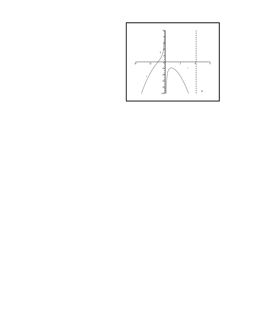
Figure 1:

Indeed, we assume that the universe is born at $t=t_{i}$ ($t_{i}<t_{1}$) and that there exists a period of time during which all energy conditions are met. It can be shown that as we approach $t_{1}$, the strong energy condition is violated first, while the weak one holds. As a result, the universe expands up to the instant $t_{1}$. At $t=t_{1}$, we obtain the de Sitter phase, but for only one instant. A forbidden zone then follows,  which should be removed by matching the solutions at $t=t_{1}$ and $t=t_{2}$. We note that this matching requires stricter conditions than those found in corresponding problems in nonrelativistic quantum mechanics based on the Schrödinger equation. Here, we require that not only the wave functions and their first derivatives but also the second derivatives be the same at the matching point. The latter is necessary to avoid discontinuities of density and pressure. The general solution of (1) has two constants of integration; therefore, it is not obvious that we can always satisfy all three conditions. But it is easy to verify that the third condition (equality of the second derivatives) follows automatically from the first two! This fortunate circumstance is a consequence of matching the solution at the inflection point of $\log\psi$. The price we pay (a discontinuity of the third derivative of the scale parameter) does not seem excessive, at least while we consider the system as a classical (i.e., not quantum) system.

Thus, controlling the zeroes of the support function of the DT, we can construct exact cosmologies with inflation. If solutions with known asymptotic characteristics (for example, evolving according to the two-thirds law) are used as initial base solutions, then the universe necessarily exits inflation, without any parameter fitting. Below, we demonstrate examples of how this approach works.

IV A simple model

The law $a\sim t^{2/3}$ gives the potential

$$V=\frac{2}{3t^{2}}.$$ (3)

The general solution of (1) with potential (3) and without a cosmological constant has the form

$$\psi^{(-)}=-\frac{c_{1}}{t}-c_{2}t^{2},$$ (4)

where $c_{1}$ and $c_{2}$ are the constants of integration. The solution describes two disconnected universes (Fig.1). The first is infinite in the past but has a singularity at $t_{0}=-(c_{1}/c_{2})^{1/3}$. The second is rather strange. It is born from a singularity at $t=t_{0}$, then expands, and undergoes superinflation, i.e., the scale parameter becomes infinite at $t=0$. Then the universe contracts, the scale parameter changing sign. Of course, this solution cannot be taken literally. The superinflation zone (to the left and right of $t=0$) is forbidden because the weak energy condition is violated in it. It is easy to find the density and pressure

$$p=-\frac{c_{1}\left(c_{1}+4c_{2}t^{3}\right)}{t^{2}\left(c_{1}+c_{2}t^{3}\right)^{2}},\qquad\rho=\frac{\left(2c_{2}t^{3}-c_{1}\right)^{2}}{3t^{2}\left(c_{1}+c_{2}t^{3}\right)^{2}}$$

Therefore, the above mentioned forbidden zone is in the interval between $t_{1}$ and $t_{2}$, where

$$\begin{array}[]{c}\displaystyle{t_{1}=\left[\left(2-\frac{3}{\sqrt{2}}\right)\frac{c_{1}}{c_{2}}\right]^{1/3}\sim-0.5\left(\frac{c_{1}}{c_{2}}\right)^{1/3}},\\ \\ \displaystyle{t_{2}=\left[\left(2+\frac{3}{\sqrt{2}}\right)^{1/3}\right]\sim 1.6\left(\frac{c_{1}}{c_{2}}\right)^{1/3}}.\end{array}$$ (5)

We consider solution (4) to hold only for $t\leq t_{1}$,where $t_{1}$ is given by (5). To continue the solution into the region $t>t_{1}$, we rewrite (4) with different constants of integration, denoted by $b_{1}$ and $b_{2}$:

$$\psi^{(+)}=\frac{b_{1}}{t}+b_{2}t^{2}.$$ (6)

For (6), the weak energy condition is violated in the interval $(t^{\prime}_{1},t^{\prime}_{2})$ where the $t^{\prime}_{1,2}$ are determined by expressions (5) with the substitutions $c_{1}\rightarrow b_{1}$ and $c_{2}\rightarrow b_{2}$. The constants $b_{1}$ and $b_{2}$ should be chosen such that they satisfy 

$$\psi^{(-)}(t_{1})=\psi^{(+)}(t_{2}^{\prime}),\qquad\dot{\psi}^{(-)}(t_{1})=\dot{\psi}^{(+)}(t_{2}^{\prime}).$$ (7)

It is noteworthy that another relation,

$$\ddot{\psi}^{(-)}(t_{1})=\ddot{\psi}^{(+)}(t_{2}^{\prime}).$$ (8)

is a consequence of (6). It thus follows that when matching $\psi^{(-)}(t_{1})$ and $\psi^{(+)}(t_{2}^{\prime})$, the density, pressure, and rate of density variation are continuous!

An obvious deficiency of this solution is a jump in time: $t_{1}\neq t_{2}^{\prime}$. Therefore, the solution is not defined on the interval $(t_{1},t_{2}^{\prime})$. But it is easy to move $t$ in $\psi^{(+)}$ and $\psi^{(-)}$ such that the two conditions that
1. the initial singularity corresponds to time $t=0$ and
2. $t_{1}=t_{2}^{\prime}$ with no jump in time.
are met. We skip the calculations and present only the final answer:

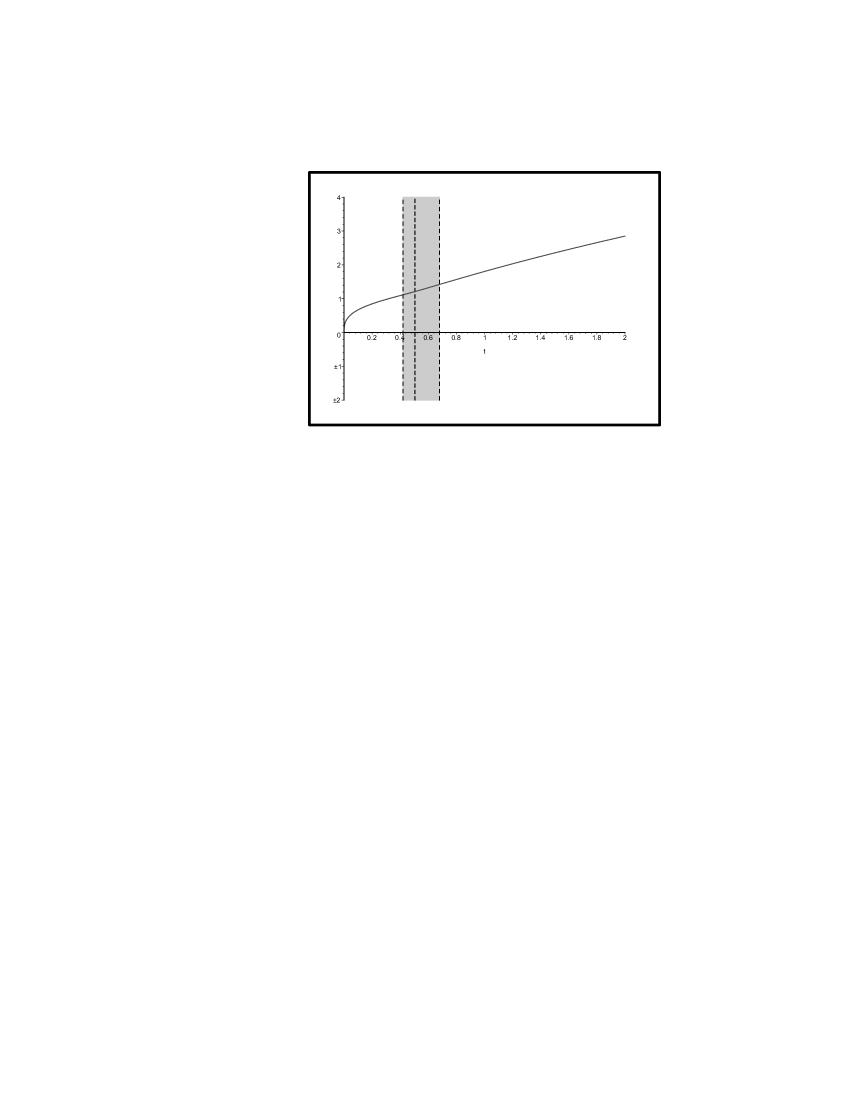
Figure 2:

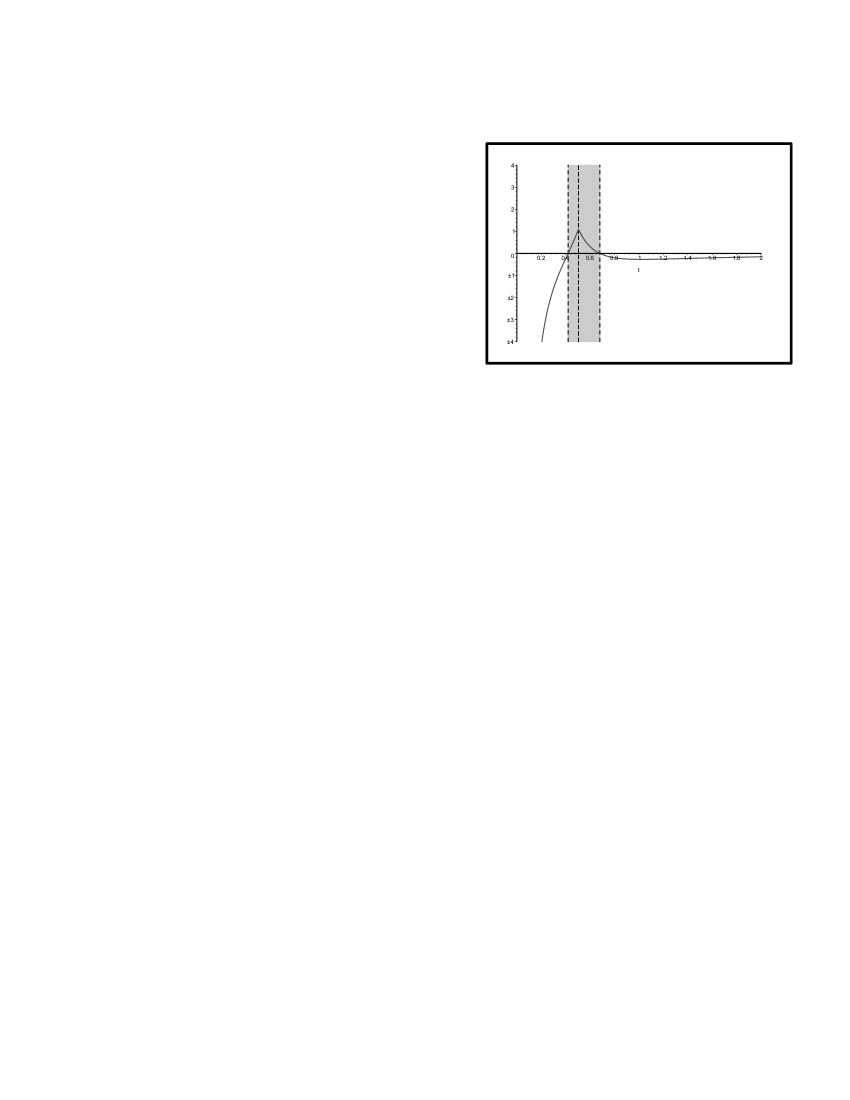
Figure 3:

1. For $0<t\leq t_{1}$, the dynamics are described by the formulas

$$\begin{array}[]{c}\displaystyle{\psi^{(-)}(t)=-\frac{c_{1}^{3}}{t-c_{1}/c_{2}}-c_{2}^{3}\left(t-c_{1}/c_{2}\right)^{2}},\\ \\ \displaystyle{V^{(-)}=\frac{2/3}{\left(t-c_{1}/c_{2}\right)^{2}}}.\end{array}$$ (9)

2.For $t_{1}<t$, the dynamics are described by the formulas

$$\begin{array}[]{c}\displaystyle{\psi^{(+)}(t)=\frac{c_{1}^{3}(3-2\sqrt{2})}{t-g}+c_{2}^{3}(3+2\sqrt{2})\left(t-g\right)^{2}},\\ \\ \displaystyle{V^{(+)}=\frac{2/3}{\left(t-g\right)^{2}}},\end{array}$$ (10)

Here,

$$\begin{array}[]{c}\displaystyle{t_{1}=\frac{c_{1}}{c_{2}}\left(1+\left(2+\frac{3}{\sqrt{2}}\right)^{1/3}\right)\sim 2.6\frac{c_{1}}{c_{2}}},\\ \\ \displaystyle{g=\frac{c_{1}}{c_{2}}\left(1+\left(16+12\sqrt{2}\right)^{1/3}\right)\sim 4.2\frac{c_{1}}{c_{2}}}.\end{array}$$ (11)

we introduce the new constants $c^{3}_{1,2}$ for convenience, and $t_{2}=t_{1}$ .The matching here is

$$\psi^{(-)}(t_{1})=\psi^{(+)}(t_{1}),\qquad{\dot{\psi}}^{(-)}(t_{1})={\dot{\psi}}^{(+)}(t_{1}),$$

$${\ddot{\psi}}^{(-)}(t_{1})={\ddot{\psi}}^{(+)}(t_{1}),\qquad V^{(-)}(t_{1})=V^{(+)}(t_{1}),$$

$$\rho^{(-)}(t_{1})=\rho^{(+)}(t_{1}),\qquad p^{(-)}(t_{1})=p^{(+)}(t_{1}).$$

The graph of $a$ as a function of $t$ for the second universe is given in Fig.2. The curve is described by the formula $a^{(-)}=\psi^{(-)}(t)$ for $t<t_{1}$ and by $a^{(+)}=\psi^{(+)}(t)$ for $t>t_{1}$,where $\psi^{(-)}(t)$ and $\psi^{(+)}(t)$ are given by (9) and (10). We specifically choose $c_{1}=c_{2}=1$. Figure 3 describes the acceleration $\ddot{a}$ as a function of time. The break is at $t=t_{1}$, given by (11).

As can be seen, inflation occurs on a finite interval (where there is a tooth on the $t$ axis).We also note that as $t\rightarrow\infty$, the potential behaves as

$$V\sim\frac{2}{3}e^{-\sqrt{3}\phi},\qquad\phi\sim\frac{2}{\sqrt{3}}\log t.$$

We have thus constructed a simple model of inflation with exit and an asymptotic transition to the Friedmann expansion era, located in the matter-dominated phase. Of course, this example does not describe our universe, because there is no oscillation phase. Neither is there secondary acceleration. But it is evident that this method can be used without fundamental difficulties to construct model cosmologies with exit without parameter fitting. Neither it is necessary to use hybrid models. We note that the solution describes another, collapsing universe with no beginning but with an end. These solutions seem rather strange, but their appearance is inevitable because the equations of general relativity are invariant under time reversal.

V The Darboux transformation

It is clear that any exact solution of (1) satisfying the energy conditions generates an exact solution of the Einstein equations in the FLRW metric. Because not all solutions $\psi$ of (1) generate a positive definite expression after substitution in the right-hand side of (2), the exact solutions of the Einstein equations are a subset of the exact solutions of (1). On the other hand, practically all exact solutions of Schrödinger equation (1) with ”physical” potentials can be constructed using a DT . Examples are the harmonic oscillator, multisoliton, and even finite-gap potentials.  We use this as an ”experimental fact” without attempting to give precise mathematical meaning to statements like ”all potentials for which Eq.(1) can be explicitly solved for all values of the spectral parameter are constructed using the DT and, possibly, an additional finite set of symmetries from other potentials with this property.” Informally speaking, we can then conclude that all exact solutions of the Einstein equations in a flat FRLW universe filled with a real scalar field can be constructed using DTs.

As a simple example, we consider potential (3), which is constructed using a single DT from a zero potential $V(0)=0$. The result of a DT applied $N$ times can be written compactly using Crum’s formulas:

$$\psi^{(N)}=\frac{\Delta_{N+1}}{\Delta_{N}},\qquad V^{(N)}=V-\frac{2}{3}\frac{d^{2}\ln\Delta_{N}}{dt^{2}},$$

where

$$\Delta_{N}=det\left[\frac{d^{k}\psi_{i}}{dt^{k}}\right],\qquad k=0,...,N-1;\qquad i=1,...,N,$$

and

$$\Delta_{N+1}=det\left[\frac{d^{k}\psi_{i}}{dt^{k}}\right],\qquad k=0,...,N;\qquad i=1,...,N+1.$$

In these expressions, the $\psi_{i}$ are particular solutions of (1) with a common initial potential $V$ and different eigenvalues $3\Lambda$. It is now clear how we can use DTs to construct models with two accelerations. We already mentioned that the potential $V^{(N)}$must have singularities. It follows from Crum’s formulas that all singularities coincide with the zeroes of functions that are contained in Crum’s determinant $\Delta_{N}$ Therefore, the problem is reduced to controlling these zeroes. We assume that the initial potential is given by (3). Solution (4) corresponds to a trivial cosmological term. The solutions of (1) with positive ($\Lambda=k^{2}/3$) and negative ($\Lambda=-k^{2}/3$) values of the lambda term are

$$\begin{array}[]{l}\displaystyle{\psi_{+}=\mu_{1}\left(1-\frac{1}{kt}\right)e^{kt}+\mu_{2}\left(1+\frac{1}{kt}\right)e^{-kt},}\\ \\ \displaystyle{\psi_{-}=\nu_{1}\left(\frac{\sin\,kt}{kt}-\cos\,kt\right)+\nu_{2}\left(\frac{\cos\,kt}{kt}+\sin\,kt\right),}\end{array}$$ (12)

where $\mu_{1,2}$ and $\nu_{1,2}$ are arbitrary constants. Using these functions for different values of $k$ in formulas (V) and regarding $\psi_{{}_{N+1}}$ as defined by (4) for all $N$, we can construct a set of solutions with the Friedmann two-thirds asymptotic behavior for $t\to+\infty$.

It is clear that the functions $\psi^{(N)}$ contain any number of singularities near which the weak energy condition is violated and acceleration therefore occurs. As in the example in Sec.3, the solutions must be cut off at the inflection points $M_{j}$ of $\log\psi^{(N)}$, where the exact de Sitter phase is realized, and matched along these points. We do not need to match solutions at adjacent points. By adjacent points, we mean points $M_{j}$ and $M_{j+1}$ between which there is only one singularity of $\psi^{(N)}$. As shown in Sec.3, we can always match any two points $M_{j}$ , which gives a degree freedom in constructing the required solution.

We note that the explicit form of the solution quickly becomes very complicated as $N$ increases. We consider some examples. Henceforth, we suppose that $c_{1}=c_{2}=1$ everywhere.

A single DT with a support function $\psi_{+}$ from (12) gives

$$\begin{array}[]{l}\displaystyle{\psi^{(1)}=\frac{\mu\left[\left(x-1\right)^{3}+k^{3}+1\right]e^{x}-\left[\left(x+1\right)^{3}+k^{3}-1\right]e^{-x}}{\mu(x-1)e^{x}+(x+1)e^{-x}},}\\ \\ \displaystyle{V^{(1)}=\frac{2k^{2}}{3}\frac{\mu^{2}e^{2x}+e^{-2x}-4\mu x^{2}-2\mu}{\left(\mu(x-1)e^{x}+(x+1)e^{-x}\right)^{2}},}\end{array}$$

where $\mu_{1}=1$, $\mu_{2}=\mu$, $x=kt$. For $\mu<0$ is given in Fig.4. Here, we already removed the regions where the weak energy condition is violated. The boundary points (where $\dot{\phi}=0$) must be matched. It is then clear that such a solution describes two universes. The first contracts to a final singularity, experiencing a time-reversed inflation at a certain instant prior to the final collapse. The dynamics of the second universe is a time reversal of the evolution of the first: it is born from a singularity, expands for some time, then undergoes inflation, exits, and settles asymptotically on the Friedmann expansion, characteristic of a matter-dominated universe.

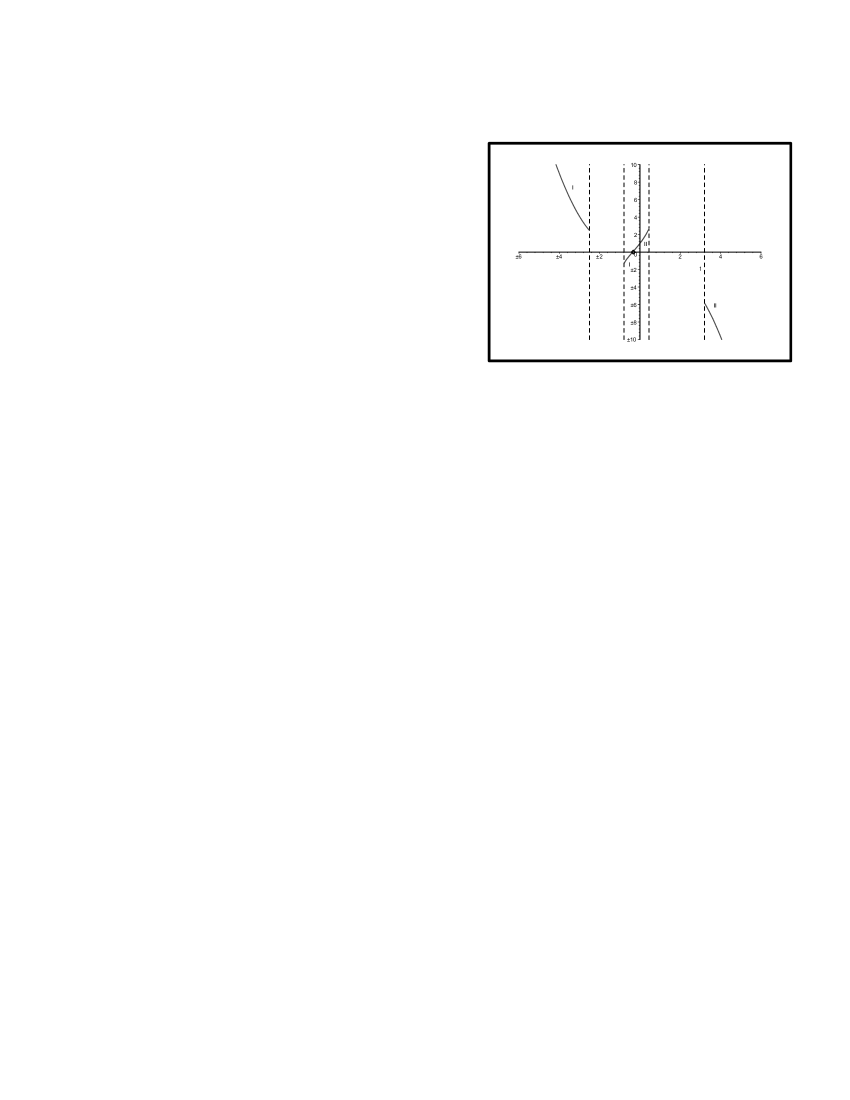
Figure 4:

A new situation arises for $\mu>0$. Figure 5 shows the graph of $\psi^{(1)}(t)$ for $\mu=2$. It demonstrates the evolution of three universes. The first collapses into a finite singularity but has no beginning. The second is born from an initial singularity, expands for some time, then begins to contract, and collapses into a final singularity (we recall that $k=0$). The third is born, expands, undergoes inflation (the boundary points are matched), and exits into a two-thirds phase.

As a final example, we present a solution obtained by a double DT (Fig.6). One support function is a solution of (1) with $\Lambda=+1/3$, $\mu_{1}=1$, $\mu_{2}=2$ and $k=1$; the other has $\Lambda=+4/3$, $\mu_{1}=1$, $\mu_{2}=3$ and $k=2$. We also have three universes here. We note that the second exists for a finite period of time, during which it undergoes inflation and then collapses. These solutions are very similar to the solutions in [11] that we mentioned at the beginning of Sec.2.

We have not attempted to construct models with two (or more) accelerations. It is clear that this problem can be solved in principle using this method. Moreover, the acceleration rate is determined by the density $\rho$; therefore, constructing potentials with several singularities, we can obtain several inflations, each with its own intensity. If the second inflation corresponds to a smaller value of $\rho$ than the first, then it is much slower. But we think that it is too early to begin constructing models using DTs. It is necessary to understand how an intermediate oscillation phase can be included. It is still unclear to us how can this be done. It is obvious that any inflation model without such a phase is impracticable. 

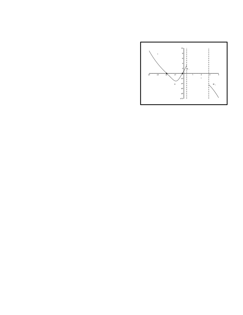
Figure 5:

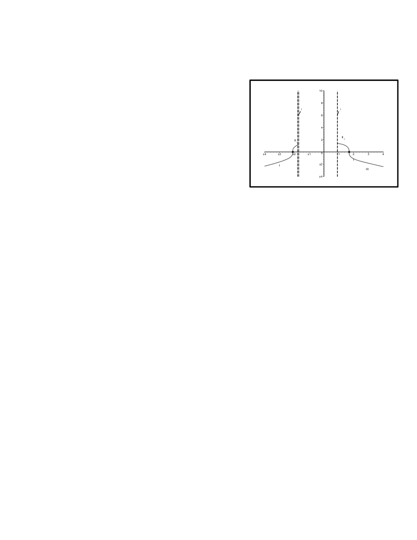
Figure 6:

VI Conclusion

We suppose that the exact solution $a(t)={}^{3}\sqrt{\psi^{(N)}(t)}$ describing two acceleration phases and an intermediate oscillation phase is constructed. We obviously encounter the problem of interpreting the potential $V^{(N)}$, which is undoubtedly hideous. It is unlikely that it can ever be described by any field theory or even string theory. Indeed, even the potentials obtained by a single DT are already too complicated and unphysical, and they are simple enough to describe even two consecutive accelerations without oscillations!

A natural reaction to the appearance of such expressions is the conclusion that real-life cosmology is not exactly solvable. From this standpoint, exact cosmologies can be useful models, but they are incapable of describing the real universe. But just how correct is this conclusion? It is quite possible that the correct potential of a self-acting scalar field is not defined by elementary particle physics but appears for a different reason. Any suppositions of this kind are speculative and unreliable. Nonetheless, we attempt to point out a source of such strange potentials outside both field theory and string theory (of the future).

According to the chaotic inflation theory of Linde, all possible vacuum states are realized in different areas of the universe, which in turn must lead to different mass spectra of the elementary particles populating these regions. In this paradigm, our region of the universe cannot be identified using physical laws alone; a certain ”weak anthropic principle” is also required. In other words, even if an all-encompassing M -theory can be constructed and it might justify our expectations, it would still prove insufficient to explain why the vacuum state of our universe is the way it is and not different, and so on.

To illustrate this picture, Linde introduces the concept of the multiuniverse[14]. In the simplest case, the multiuniverse can be described as an infinite sum over all possible actions describing all possible quantum field theories and M -theories.  Even though hypotheses of this kind can seem speculative, it must be borne in mind that all existing explanations of the observed density of the vacuum energy ($\sim 0.7\rho_{c}$) have been obtained using the anthropic principle, which apparently makes sense only if the multiuniverse hypothesis is true. 

If we accept this hypothesis, then it is clear that the existence of regions with the strangest self-acting potentials is possible. In this case, we must readdress the basic questions we normally ask. For example, potentials $V(\phi)$ are generally taken from particle theory ($V\sim\phi^{2}$ and $V\sim\phi^{4}$) or string theory $V\sim e^{\alpha\phi}$. Why these and not $V\sim\phi^{8}$, for example? Because a theory with such a potential is nonrenormalizable for $d=4$. We have every reason to believe that a nonrenormalizable theory is a ”bad” theory because it requires a new Lagrangian on each new scale and therefore contains an infinite number of indefinite parameters as a rule. As well as being renormalizable, models must also satisfy other generally known properties: unitary, a Hamiltonian bounded from below, etc.

We now suppose that we have succeeded in constructing a family of potentials giving an evolution of the universe consistent with observations (for example, using DTs). The next step would be to check these models using the methods of quantum theory (renormalizability, etc.). If one of these potentials satisfies the appropriate checks, then we can perfectly well use it even though we did not obtain it using the basic principles of field theory or string theory. We obtained it using the multiuniverse concept, and field theory (or string theory) is only required to verify its consistency.

REFERENCES

1. A. H. Guth, ”The Inflationary Universe: A Possible Solution To The Horizon And Flatness Problems,” Phys. Rev. D 23, 347 (1981).
2. A. D. Linde, ”A New Inflationary Universe Scenario: A Possible Solution Of The Horizon, Flatness, Homogeneity, Isotropy And Primordial Monopole Problems,” Phys. Lett. B 108, 389 (1982); A. Albrecht and P. J. Steinhardt, ”Cosmology For Grand Unifed Theories With Radiatively Induced Symmetry Breaking,” Phys. Rev. Lett. 48, 1220 (1982).
3. A.D. Linde, ”Chaotic Inflation,” Phys. Lett. 129B, 177 (1983).
4. S. Perlmutter et al. [Supernova Cosmology Project Collaboration], Astrophys. J. 517, 565 (1999) [arXiv:astro-ph/9812133]; A. G. Riess et al. [Supernova Search Team Collaboration], Cosmological Constant,” Astron. J. 116, 1009 (1998) [arXiv:astro-ph/9805201]; P. M. Garnavich et al., Astrophys. J. 509, 74 (1998) [arXiv:astro-ph/9806396].
5. T.P. J. Steinhardt, L. M. Wang and I. Zlatev, Phys. Rev. D 59, 123504 (1999) [arXiv:astro-ph/9812313]; B. Ratra and P. J. Peebles, ”Cosmological Consequences Of A Rolling Homogeneous Scalar Field,” Phys. Rev. D 37, 3406 (1988); I. Zlatev, L. M. Wang and P. J. Steinhardt, ”Quintessence, Cosmic Coincidence, and the Cosmological Constant,” Phys. Rev. Lett. 82, 896 (1999) [arXiv:astro-ph/9807002].
6. Justin Khoury, Burt A. Ovrut, Paul J. Steinhardt and Neil Turok. ”The ekpyrotic universe: colliding branes and the origin of the hot big bang.” Phys. Rev. D64: 123522, 2001. [arXiv:hep-th/0103239].
7. P. J. Steinhardt and N. Turok, ”Cosmic evolution in a cyclic universe,” Phys. Rev. D 65, 126003 (2002) [arXiv:hep-th/0111098]; P. J. Steinhardt and N. Turok, ”A cyclic model of the universe,” [arXiv:hep-th/0111030]; P. J. Steinhardt and N. Turok, ”Is Vacuum Decay Significant in Ekpyrotic and Cyclic Models?” [arXiv:astro-ph/0112537].
8. R. Dick, ”Brane worlds”, Class. and Quantum Grav., V. 18, N. 7, R1-24 (2001) [arXiv:hep-th/0105320].
9. R. Kallosh, L. Kofman and A. Linde, ”Pyrotechnic universe”. Phys. Rev. D64: 123523, 2001. [arXiv:hep-th/0104073]; D. H. Lyth, ”The failure of cosmological perturbation theory in the new ekpyrotic scenario,” [arXiv:hep-ph/0110007];R. Brandenberger and F. Finelli, ”On the spectrum of fluctuations in an effective field theory of the ekpyrotic universe,” arXiv:hep-th/0109004.
10. Yu. V. Baryshev, ”Conceptual Problems Of Fractal Cosmology”, Astronomical and Astrophysical Transaction, Vol. 19, pp. 417-435 (2000).
11. G. Felder, A. Frolov, L. Kofman and A. Linde, ”Cosmology With Negative Potentials” [arXiv: hep- th/ 0202017]
12. R. Kallosh, A. D. Linde, S. Prokushkin and M. Shmakova, ”Gauged supergravities, de Sitter space and cosmology,” Phys. Rev. D 65, 105016 (2002) [arXiv:hep-th/0110089]; A. Linde, ”Fast-roll inflation”, JHEP 0111, 052 (2001) [arXiv:hep-th/0110195].
13. J. D. Barrow, ”Exact Inflationary Universes With Potential Minima”, Phys. Rev. D 49 3055 (1994); R. Maartens, D. R. Taylor and Roussos, ”Exact Inflationary Cosmologies With Exit”, Phys. Rev. D 52 3358 (1995);); V. M. Zhuravlev, S. V. Chervon, and V. K. Shchigolev, JETP, 87, 223 (1998); S. V. Chervon,V. M. Zhuravlev, and V. K. Shchigolev, Phys. Lett. B, 398, 269 (1997); J. D. Barrow, Phys. Lett. B, 235,40 (1990); G. F. R. Ellis and M. S. Madsen, Class. Q. Grav., 8, 667 (1991); J. E. Lidsey, Class. Q. Grav., 8, 923 (1991);J. D. Barrow and P. Saich, Class. Q. Grav., 10, 279 (1993); P. Parson and J. D. Barrow, Class. Q. Grav., 12, 1715 (1995).
14. A. D. Linde, Phys. Lett. B, 200, 272 (1988); Particle Physics and In?ationary Cosmology, Harwood, Chur, Switzerland (1990).
15. V. M. Zhuravlev and S. V. Chervon, JETP, 91, 227 (2000).
16. A.V. Yurov, ”Exact Inflationary Cosmologies With Exit: From An Inflaton Complex Field To An Anti-Inflaton One”, Class. Quantum Grav., 18, 3753 (2001).
17. A. Kamenshchik, U. Moschella and V. Pasquier, ”An Alternative To Quintessence” [arXiv: gr-qc/0103004].
18. A. D. Linde,”Hybrid inflation,” Phys. Rev. D 49, 748 (1994) [arXiv:astro-ph/9307002].
19. V. B. Matveev V B and Salle M A   1991 Darboux Transformation and Solitons (Berlin–Heidelberg: Springer Verlag)
20. J. G. Darboux, C.R.Acad.Sci.,Paris 94 p.1456 (1882).
21. M. M. Crum, ”Associated Sturm-Liouville equations”, Quart. J. Math. Oxford 6 2 p. 121 (1955).
22. F. J. Tipler and J. Graber, ”Closed Universes With Black Holes But No Event Horizons As a Solution to the Black Hole Information Problem”, [arXiv:gr- qc/ 0003082].
23. V. E. Adler, Theor. Math. Phys., 101, No. 3, 1381 (1995).
24. A. P. Veselov and A. B. Shabat, Funct. Anal. Appl., 27, No. 2, 81 (1993).
25. A. D. Linde, “The Universe Multiplication And The Cosmological Constant Problem,” Phys. Lett. B 200, 272 (1988); A.D. Linde, Particle Physics and Inflationary Cosmology (Harwood, Chur, Switzer-land, 1990).
26. M. Tegmark, ”Is ’the theory of everything’ merely the ultimate ensemble theory?”, Annals Phys. 270, 1 (1998) [arXiv:gr-qc/9704009].
27. H. B. Nielsen and C. Froggatt, ”Influence from the Future” [arXiv: hep- ph/ 9607375]