Dark Energy: Vacuum Fluctuations, the Effective Phantom Phase,
and Holography

Abstract

We aim at the construction of dark energy models without exotic matter but with a phantom-like equation of state (an effective phantom phase). The first model we consider is decaying vacuum cosmology where the fluctuations of the vacuum are taken into account. In this case, the phantom cosmology (with an effective, observational $\omega$ being less than $-1$ ) emerges even for the case of a real dark energy with a physical equation of state parameter $\omega$ larger than $-1$. The second proposal is a generalized holographic model, which is produced by the presence of an infrared cutoff. It also leads to an effective phantom phase, which is not a transient one as in the first model. However, we show that quantum effects are able to prevent its evolution towards a Big Rip singularity.

I Introduction

Recent observational constraints obtained for the dark energy equation of state (EOS) indicate that our Universe is probably in a superaccelerating phase (dubbed as “phantom cosmology”), i.e. $\dot{H}>0$ (see ywang and references therein). When dark energy is modeled as a perfect fluid, it can be easily found that in order to drive a phantom cosmology, the dark energy EOS should satisfy $\omega_{d}\equiv\rho_{d}/p_{d}<-1$ (phantom) caldwell . The classical phantom has already many similarities with a quantum field NO . However, it violates important energy conditions and all attempts to consider it as a (quantum) field theory show that it suffers from instabilities both from a quantum mechanical and from a gravitational viewpoint carroll-phantom . Thermodynamics of this theory are also quite unusual brevik ; odintsov-de : the corresponding entropy must be negative or either negative temperatures must be introduced in order to obtain a positive entropy. The typical final state of a phantom universe is a Big Rip singularity bigrip which occurs within a finite time interval. (Note that quantum effects coming from matter may slow up or even prevent the Big Rip singularity odintsov ; odintsov-de , which points towards a transient character of the phantom era).

In the light of such problems, we feel that it would be very interesting to construct a new scenario where an (effective) phantom cosmology could be described through more consistent dark energy models with $\omega_{d}\geq-1$. Recently, some proposals along this line have already appeared. An incomplete list of them includes the consideration of modified gravity abdalla or generalized gravity carroll-trick , taking into account quantum effects Onemli , non-linear gravity-matter couplings couple , the interaction between the photon and the axion csaki , two-scalar dark energy models odintsov ; hu , the braneworld approach (for a review, see sahni , however, FRW brane cosmology may not be predictive boundary ), and several others.

In this paper we continue the construction of more consistent dark energy models, with an effective phantom phase but without introducing the phantom field, what is realized by using a number of considerations from holography and vacuum fluctuations. In the next section, a dark energy model which includes vacuum fluctuations effects (a decaying vacuum cosmology) is considered. With reasonable assumptions about the vacuum decaying law, the FRW equations are modified. Then, it is shown that the effective dark energy EOS parameter, which is constrained by astrophysical observations, is less than $-1$. However, even if the dark energy EOS parameter is actuall bigger than $-1$, the modified FRW expansion, or in other words, a decaying vacuum can trick us into thinking about some exotic matter with $w$ less than $-1$. Hence, such dark energy model does not need the exotic phantom matter, its effective phantom phase is transient and it does not contain a Big Rip singularity. In section 3 another holographic dark energy model which uses the existence of an infrared cutoff, identified with a particle or future horizon, is constructed. It generalizes some previous attempts in this direction and leads to modified FRW dynamics. Such model also contains an effective phantom phase (without introduction of a phantom field), which leads to Big Rip type singularity. However, taking into account matter quantum effects may again prevent (or moderate) the Big Rip emergence, in the same way as in Refs. odintsov ; odintsov-de . A summary and outlook is given in the Discussion section.

II Dark energy and vacuum fluctuations

When considering the energy of the vacuum, there are two conceptually different contributions: the energy of the vacuum state and the energy corresponding to the fluctuations of the vacuum. More precisely, the first is the eigenvalue of the Hamiltonian acting on the vacuum state: $E=\langle 0|H|0\rangle$, while the second is the dispersion of the Hamiltonian: $E_{\Delta}=\langle 0|H^{2}|0\rangle-(\langle 0|H|0\rangle)^{2}$.

In constructing the dark energy as a scalar field (“quintessence”) quint , only the energy of the vacuum state is actually considered, and the vacuum fluctuations are neglected. Note that, while the potential energy of the scalar field corresponds to the energy of the vacuum state, the kinetic energy density does not correspond to the energy of the vacuum fluctuations. The kinetic energy corresponds to the energy of the excited states. Actually, ignoring vacuum fluctuations may not be a well justified assumption. It was ignored for quintessence models, just for simplicity.

Thus, confronted with the difficulties of building a phantom universe from quintessence alone, it is natural to consider the sector which was ignored before. In this paper, we will show that the ignored sector can really help to resolve the problems above. The key point is that, when considering those two contributions to the vacuum energy in a cosmological setup, their energy density changes with the cosmological expansion in different ways.

First, if dark energy is modeled as a scalar field $\phi$, interacting only with itself and with gravity quint , then it behaves just like an ordinary perfect fluid satisfying the continuity equation

$$\dot{\rho}_{d}+3H(\rho_{d}+p_{d})=0,$$ (1)

where

$$\rho_{d}={1\over 2}\dot{\phi}^{2}+V(\phi),$$ (2)

and

$$p_{d}={1\over 2}\dot{\phi}^{2}-V(\phi).$$ (3)

Thus

$$\omega_{d}=\frac{{1\over 2}\dot{\phi}^{2}-V(\phi)}{{1\over 2}\dot{\phi}^{2}+V(\phi)}\geq-1.$$ (4)

When comparing dark energy models with observations, it is often assumed that $\omega_{d}=\text{const.}$ (this is reasonable since allowing EOS to vary will increase the number of parameters to constrain). Then from equation (1) it follows that

$$\rho_{d}\propto(1+z)^{3(1+\omega_{d})}.$$ (5)

On the other hand, to find the energy corresponding to the fluctuations of the vacuum, we must have a regularization scheme in order to handle the divergent expression brustein . Since the regularization scheme must be Lorentz invariant (as is the case, e.g. of dimensional regularization in curved spacetime), it turns out that the final result must be of the form $T_{\Lambda\mu\nu}=\rho_{\Lambda}g_{\mu\nu}$ even if $\rho_{\Lambda}$ is time-varying due to the time variation of the IR cutoff pad . Note that mathematically, $\rho_{\Lambda}g_{\mu\nu}$ is exactly the energy-momentum of a perfect fluid with $p=-\rho$. Then from the energy-momentum conservation law, we find that the vacuum fluctuations will interact with matter brostein ; wang ; horvat

$$\dot{\rho}_{m}+3H\rho_{m}=-\dot{\rho}_{\Delta},$$ (6)

where $\rho_{m}$ is the energy density of nonrelativistic matter and $\rho_{\Delta}$ is the energy density of vacuum fluctuations. Following wang , we will call a cosmological model which includes the effects of vacuum fluctuations a “decaying vacuum cosmology” since, as can be seen from (6), during the expansion of the Universe, owing to the fact that $\rho_{\Delta}$ is decreasing, new matter is created from the vacuum.

It is clear that Eq. (6) and the Friedmann equation are not enough to describe a decaying vacuum cosmology. We should also specify a vacuum decaying law. There are lots of papers on various proposals concerning how $\rho_{\Delta}$ will change with cosmological time (see wang and references therein). However, recently it has been proposed wang that from (6) and a simple assumption about the form of the modified matter expansion rate, the vacuum decaying law can be constrained to a two-parameter family. Thus, we can think about the observational consequences of a decaying vacuum cosmology, even if we do not understand the physics underlying the decaying law. More precisely, the main (and rather natural) assumption is that the matter expansion rate be of the form

$$\rho_{m}=\rho_{m0}a^{-3+\epsilon}\ .$$ (7)

where $\rho_{m0}$ is the present value of $\rho_{m}$. Actually, this assumption is valid in all the existing models of a decaying vacuum cosmology. An immediate simple observation is that one must have $\epsilon\leq 1$. Otherwise, the Universe would expand with an acceleration in the matter dominated era, which is excluded by the observations of SNe Ia, that our Universe expanded with deceleration before redshift $z\sim 0.5$ ywang . Actually, it is expected that $\epsilon\ll 1$ since, so far, there has been no observational evidence about an anomalous dark matter expansion rate.

From (6) and (7), we can find that $\rho_{\Delta}$ is given by

$$\rho_{\Delta}=\tilde{\rho}_{\Delta 0}+{\epsilon\rho_{m0}\over 3-\epsilon}a^{-3+\epsilon}\ ,$$ (8)

where $\tilde{\rho}_{\Delta 0}$ is an integration constant. In wang it was shown that all the existing vacuum decaying laws can be described by a suitable choice of $\epsilon$ and $\tilde{\rho}_{\Delta}$. In our current framework, the term $\tilde{\rho}_{\Delta}$ can be absorbed into the dark energy density, so in the following discussion, we will simply assume $\tilde{\rho}_{\Delta}=0$. The FRW equation describing a Universe consisting of cold dark matter, dark energy and vacuum fluctuations is

$$H^{2}={1\over 3M_{P}^{2}}(\rho_{m}+\rho_{d}+\rho_{\Delta}).$$ (9)

It is important to note that due to the modified dark matter expansion rate, the physical dark energy EOS $\omega_{d}$ is no longer the one directly seen in supernova observations. To compare our model with observations, we can adopt the framework of effective dark energy EOS linder that can unify quintessence, modified gravity, and decaying vacuum cosmology into one and a single framework. The effective dark energy EOS is defined as linder

$$\omega_{eff}=-1+{1\over 3}\frac{d\ln\delta H^{2}(z)}{d\ln(1+z)}\ ,$$ (10)

where $\delta H^{2}\equiv H^{2}-\rho_{m0}(1+z)^{3}/(3M_{P}^{2})$ characterizes any contribution to the cosmic expansion in addition to the standard cold dark matter. It is $\omega_{eff}$ that is the real quantity which is constrained in cosmological observations. The explicit form of $\delta H^{2}$ in the above model is

$${\delta H^{2}(z)\over H_{0}^{2}}={3\Omega_{m0}\over 3-\epsilon}(1+z)^{3-\epsilon}-\Omega_{m0}(1+z)^{3}+\Omega_{d0}(1+z)^{3(1+\omega_{d})},$$ (11)

from which we can find the effective dark energy EOS:

$$\omega_{eff}(z)=\omega_{d}+\frac{\omega_{d}(1+z)^{3}-{3\omega_{d}+\epsilon\over 3-\epsilon}(1+z)^{3-\epsilon}}{{3\over 3-\epsilon}(1+z)^{3-\epsilon}-(1+z)^{3}+{\Omega_{d0}\over\Omega_{m0}}(1+z)^{3(1+\omega_{d})}}.$$ (12)

From this one can see that, ignoring the decay of the vacuum, i.e. with $\epsilon=0$, then $\omega_{eff}=\omega_{d}$.

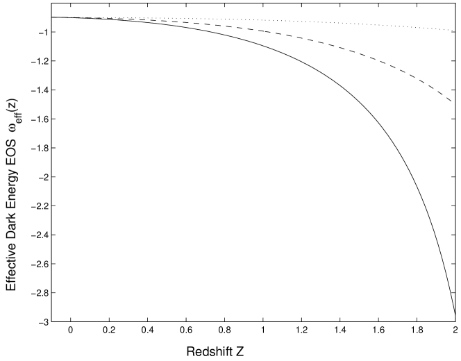
Figure 1: Evolution of the effective dark energy EOS as given by equation (12) with $\omega_{d}=-0.9$. Dotted, dashed and solid lines correspond to $\epsilon=0.01,0.05,0.1$, respectively.

FIG. 1 shows the evolution of $\omega_{eff}$ up to redshift 2 for $\epsilon=0.01,\omega_{d}=0.9$ from top to bottom. It is easy to see that $\omega_{eff}=\omega_{d}$ for small $z$ and negative $z$. As mentioned above, in current works constraining $\omega_{eff}$, the most reliable assumption is that $\omega_{eff}$ is a constant ywang . Thus, what is actually constrained in those works is the average value of the effective EOS $\bar{\omega}_{eff}\equiv\int\Omega_{eff}(a)\omega_{eff}(a)da/\int\Omega_{eff}(a)da$ limin , which from FIG. 1 is smaller than $-1$ if averaged up to redshift 2 (the current upper bound on observable supernova) for roughly $\epsilon>0.05$. Thus, we have constructed a model which can drive a phantom cosmology with a physical EOS larger than $-1$. In this picture, $\bar{\omega}_{eff}<-1$ is not the result of exotic behavior of the dark energy, but the modified expansion rate of the CDM, i.e. a decaying vacuum can trick us into thinking that $\omega_{eff}<-1$. Under the assumption of a constant EOS, the current constraint on $\bar{\omega}_{eff}$ from SNe Ia data is $-4.36<\bar{\omega}_{eff}<0.8$ at $95\%$ C.L. ywang . Then $\epsilon<0.1$ is obviously consistent with current constraints on dark energy EOS. Moreover, it is easy to see from FIG. 1 that $\bar{\omega}_{eff}$ will be more and more negative when the redshift gets larger. Thus, if more high redshift SNe Ia data become available in the future, the interaction between vacuum and nonrelativistic matter predicts that we will get a more negative value for $\bar{\omega}_{eff}$.

It is also interesting to note that in the current model, the arguments leading to a Big Rip of the Universe in a phantom cosmology bigrip no longer apply. While the current expansion rate is superaccelerating, the Universe will be driven by only the healthy $\omega_{X}\geq-1$ dark energy in the future. The Universe is now superaccelerating just because non-relativistic matter is of the same order of magnitude as dark energy, and thus the effects of the nonstandard expansion rate of nonrelativistic matter cannot be ignored. This conclusion is supported by recent analysis on the construction of a sensible quantum gravity theory in cosmological spacetime bousso . Actually, it is easy to see that the trouble with de Sitter space discussed in bousso will be avoided in a superaccelerating cosmology: the total amount of Hawking radiation due to the cosmological horizon is infinite and thus it will thermalize the observer. Furthermore, since the horizon is decreasing in a superaccelerating cosmology, black holes will dominate the spectrum of thermal fluctuations in late time bousso . An observer may be swallowed by a horizon sized black hole before he/she can reach the Big Rip singularity. Thus, it is doubtful that the appearance of Big Rip singularity makes sense in the quantum gravity theory. This is also supported by a direct account of the quantum gravity effects moderating or preventing the Big Rip odintsov ; odintsov-de .

In the above discussion, the simplest model of dark energy characterized by a constant EOS is considered with the assumption that the vacuum decays only to dark matter. Let us now discuss a more general case. Let the vacuum fluctuation energy decay into both dark matter and dark energy. Specifically, we will consider a dark energy with EOS proposed in odintsov-de (see, also stefa ; odintsov ),

$$p_{d}=-\rho_{d}-A\rho_{d}^{\alpha},$$ (13)

where $A$ and $\alpha$ are constant. This can be viewed as characterizing the minimum deviation of the dark energy EOS from that of a cosmological constant.

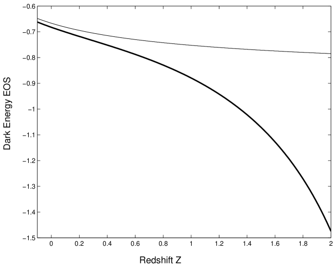
Figure 2: Evolution of the physical (thin line) and effective (thick line) dark energy EOS as given by equations (19) and (18).

When considering the effect of vacuum fluctuations, from the total energy-momentum conservation, one gets

$$\dot{\rho}_{d}+\dot{\rho}_{m}+3H(\rho_{d}+p_{d}+\rho_{m})=-\dot{\rho}_{\Delta}.$$ (14)

Now one cannot proceed further without specifying a vacuum decaying law. Currently, the following law can be proposed

$$\rho_{\Delta}=\epsilon M_{P}^{2}H^{2}.$$ (15)

This law can be deduced from the results of brustein , in which the vacuum fluctuations of a spatially finite quantum system, e.g. free scalar field, have been evaluated. The most interesting conclusion in this computation is that the energy corresponding to the vacuum fluctuations is proportional to the area of the spatial boundary of the system. In a cosmological setting, it is reasonable to view the Hubble horizon as the spatial boundary of the quantum theory describing matter in the Universe.

From equation (15) and the Friedmann equation, it can be shown that Eq. (14) can be written as

$$\dot{\rho}_{d}+\dot{\rho}_{m}+(3-\epsilon)H(\rho_{d}+p_{d}+\rho_{m})=0,$$ (16)

from which we find that

$$\rho_{d}=\rho_{d0}[1-(3-\epsilon)\tilde{A}(1-\alpha)\ln(1+z)]^{1/(1-\alpha)},\ \ \rho_{m}=\rho_{m0}(1+z)^{3-\epsilon},$$ (17)

where $\tilde{A}\equiv A\rho_{d0}^{\alpha-1}$. For $\epsilon=0$, i.e. in the absence of vacuum decaying effects, (17) reduces to the expression found in stefa ; odintsov .

Now, one can find the effective dark energy EOS by exactly the same procedure as above:

$$\omega_{eff}=-1+\frac{(1+z)^{3-\epsilon}-(1+z)^{3}-{(3-\epsilon)\tilde{A}\Omega_{d0}\over 3\Omega_{m0}}(1-(3-\epsilon)\tilde{A}(1-\alpha)\ln(1+z))^{\alpha/(1-\alpha)}}{{3\over 3-\epsilon}(1+z)^{3-\epsilon}-(1+z)^{3}+{\Omega_{d0}\over\Omega_{m0}}(1-(3-\epsilon)\tilde{A}(1-\alpha)\ln(1+z))^{1/(1-\alpha)}},$$ (18)

When $\epsilon=0$, this reduces to the physical equation of state,

$$\omega_{d}={p_{d}\over\rho_{d}}=-1-\tilde{A}(1-3\tilde{A}(1-\alpha)\ln(1+z))^{-1}.$$ (19)

FIG. 2 shows the evolution of $\omega_{eff}$ and $\omega_{d}$ up to redshift 2 for $\tilde{A}=-1/3,\alpha=1/2,\epsilon=0.1$. Hence, it is obvious that while $\omega$ for the physical dark energy EOS is larger than $-1$, with account of vacuum fluctuations, for the dark energy EOS is smaller than $-1$. Thus, we have constructed a vacuum fluctuation dark energy model where the phantom phase is transient and there is no need to introduce exotic matter (a phantom) to comply with the observational data.

III Holographic dark energy and the phantom era

The fluctuations of the vacuum energy are caused by quantum effects. It is expected, that the quantum corrections to the theories coupled with gravity should be constrained by the holography. The holography requires an infrared cutoff $L_{\Lambda}$, which has dimensions of length and could be dual to the ultraviolet cutoff. Hence, the fluctuations of the vacuum energy are naturally proportional to the inverse square of the infrared cutoff. This points to the connection of dark energy based on fluctuations of the vacuum energy with the holographic dark energy. Our purpose here will be to construct the generalization of the holographic dark energy model which naturally contains the effective phantom phase.

Let us start from the holographic dark energy model which is a generalization of the model in Li (see also Myung1 ; Myung2 ; FEH ). Denote the infrared cutoff by $L_{\Lambda}$, which has a dimension of length. If the holographic dark energy $\rho_{\Lambda}$ is given by,

$$\rho_{\Lambda}=\frac{3c^{2}}{\kappa^{2}L_{\Lambda}^{2}}\ ,$$ (20)

with a numerical constant $c$, the first FRW equation $(H^{2}/\kappa^{2})=\rho_{\Lambda}$ can be written as

$$H=\frac{c}{L_{\Lambda}}\ .$$ (21)

Here it is assumed that $c$ is positive to assure the expansion of the universe. The particle horizon $L_{p}$ and future horizon $L_{f}$ are defined by

$$L_{p}\equiv a\int_{0}^{t}\frac{dt}{a}\ ,\quad L_{f}\equiv a\int_{t}^{\infty}\frac{dt}{a}\ .$$ (22)

For the FRW metric with the flat spacial part:

$$ds^{2}=-dt^{2}+a(t)^{2}\sum_{i=1,2,3}\left(dx^{i}\right)^{2}\ .$$ (23)

Identifying $L_{\Lambda}$ with $L_{p}$ or $L_{f}$, one obtains the following equation:

$$\frac{d}{dt}\left(\frac{1}{aH}\right)=\pm\frac{c}{a}\ .$$ (24)

Here, the plus (resp. minus) sign corresponds to the particle (resp. future) horizon. Assuming

$$a=a_{0}t^{h_{0}}\ ,$$ (25)

it follows that

$$h_{0}=1\mp c\ .$$ (26)

Then, in the case $L_{\Lambda}=L_{f}$, the universe is accelerating ($h_{0}>0$ or $w=-1+{2}/{3h_{0}}<-1/3$). When $c>1$ in the case $L_{\Lambda}=L_{p}$, $h_{0}$ becomes negative and the universe is shrinking. If the theory is invariant under the change of the direction of time, one may change $t$ with $-t$. Furthermore by properly shifting the origin of time, we obtain, instead of (25),

$$a=a_{0}\left(t_{s}-t\right)^{h_{0}}\ .$$ (27)

This tells us that there will be a Big Rip singularity at $t=t_{s}$. Since the direction of time is changed, the past horizon becomes a future like one:

$$L_{p}\to\tilde{L}_{f}\equiv a\int_{t}^{t_{s}}\frac{dt}{a}=a\int_{0}^{\infty}\frac{da}{Ha^{2}}\ .$$ (28)

Note that if $L_{\Lambda}$ is chosen as a future horizon in (22), the deSitter space

$$a=a_{0}{\rm e}^{\frac{t}{l}}\quad\left(H=\frac{1}{l}\right)$$ (29)

can be a solution. Since $L_{f}$ is now given by $L_{f}=l$, we find that the holographic dark energy (20) is given by $\rho_{\Lambda}=\frac{c^{2}}{\kappa^{2}l^{2}}$. Then when $c=1$, the first FRW equation $\frac{3}{\kappa^{2}}H^{2}=\rho_{\Lambda}$ is identically satisfied. If $c\neq 1$, the deSitter solution is not a solution. If we choose $L_{\Lambda}$ to be the past horizon, the deSitter solution does not exist, either, since the past horizon $L_{p}$ (22) is not a constant: $L_{p}=(1-{\rm e}^{\frac{t}{l}})/l$.

In Hsu , it has been argued that, when we choose $L_{\Lambda}$ to be the particle horizon $L_{p}$, the obtained energy density gives a natural value consistent with the observations but the parameter $w$ of the equation of the state vanishes since $L_{p}$ should behave as $a(t)^{3/2}$. That seems to contradict with the observed value. In the present paper, we wish to generalize the holographic model to have, hopefully, more freedom and to be more successful in cosmology. As we will see in this section, there may be many possiblilities for the choice of the infrared cutoff $L_{\Lambda}$ which are more consistent with observations (giving correct cosmology without above problems).

In general, $L_{\Lambda}$ could be a combination (a function) of both, $L_{p}$, $L_{f}$. Furthermore, if the span of life of the universe is finite, the span $t_{s}$ can be an infrared cutoff. If the span of life of the universe is finite, the definition of the future horizon $L_{f}$ (22) is not well-posed, since $t$ cannot go to infinity. Then, we may redefine the future horizon as in (28)

$$L_{f}\to\tilde{L}_{f}\equiv a\int_{t}^{t_{s}}\frac{dt}{a}=a\int_{0}^{\infty}\frac{da}{Ha^{2}}\ .$$ (30)

Since there can be many choices for the infrared cutoff, one may assume $L_{\Lambda}$ is the function of $L_{p}$, $\tilde{L}_{f}$, and $t_{s}$, as long as these quantities are finite:

$$L_{\Lambda}=L_{\Lambda}\left(L_{p},\tilde{L}_{f},t_{s}\right)\ .$$ (31)

As an example, we consider the model

$$\frac{L_{\Lambda}}{c}=\frac{2t_{s}\left(\frac{L_{p}+\tilde{L}_{f}}{\pi t_{s}}\right)^{2}}{\left\{1+\left(\frac{L_{p}+\tilde{L}_{f}}{\pi t_{s}}\right)^{2}\right\}^{2}}\ ,$$ (32)

which leads to the solution:

$$H=\frac{1}{2}\left(\frac{1}{t}+\frac{1}{t_{s}-t}\right)\ ,\quad\mbox{or}\quad a=a_{0}\sqrt{\frac{t}{t_{s}-t}}\ .$$ (33)

In fact, one finds

$$L_{p}+\tilde{L}_{f}=a\int_{0}^{\infty}\frac{da}{Ha^{2}}=a\int_{0}^{t_{s}}\frac{dt}{a}=\pi t_{s}\sqrt{\frac{t}{t_{s}-t}}\ ,$$ (34)

and therefore

$$\frac{c}{L_{\Lambda}}=\frac{1}{2}\left(\frac{1}{t}+\frac{1}{t_{s}-t}\right)=H\ ,$$ (35)

which satisfies (21).

We should note that any kind of finite large quantity could be chosen as the infrared cutoff. For instance, $L_{\Lambda}$ could depend on $dL_{p}/dt$ and/or $d{\tilde{L}}_{f}/dt$. The following model may be considered:

$$\frac{\tilde{c}}{L_{\Lambda}}=\frac{1}{L_{p}+\tilde{L}_{f}}\left(\frac{dL_{p}}{dt}+\frac{d\tilde{L}_{f}}{dt}\right)\ ,$$ (36)

with the assumption that

$$\tilde{c}\equiv\int_{0}^{\infty}\frac{da}{Ha^{2}}=\int_{0}^{t_{s}}\frac{dt}{a}$$ (37)

is finite. Since $\tilde{c}$ is a constant and $L_{p}+\tilde{L}_{f}=a\tilde{c}$, from (36), we find that (21) is trivially satisfied. Therefore, in the model (36), as long as $\tilde{c}$ in (37) is finite, an arbitrary FRW metric is a solution of (21).

The next step is to consider the combination of the holographic dark energy and other matter with the following EOS

$$p=-\rho-f(\rho)\ .$$ (38)

The holographic dark energy is given by (20) with $L_{\Lambda}=L_{p}$, $L_{f}$ in (22), or $\tilde{L}_{f}$ in (28) or (30). Then from the first FRW equation

$$\pm\frac{d}{dt}\left\{\frac{c}{a}\left(H^{2}-\frac{\kappa^{2}}{3}\rho\right)^{-\frac{1}{2}}\right\}=\frac{1}{a}\ .$$ (39)

First, we consider the case when $f(\rho)=-(1+w)\rho$ with constant $w$, that is,

$$p=w\rho\ .$$ (40)

Then, by using the conservation of the energy

$$0=\frac{d\rho}{dt}+3H\left(\rho+p\right)\ ,$$ (41)

it follows

$$\rho=\rho_{0}a^{-3(1+w)}\ .$$ (42)

By combining (39) with (42), one finds a solution

$$a=\left\{\begin{array}[]{lll}a_{0}t^{\frac{2}{3(1+w)}}&\mbox{when}&w>-1\\ a_{0}\left(t_{s}-t\right)^{\frac{2}{3(1+w)}}&\mbox{when}&w<-1\\ \end{array}\right.$$ (45)

$$\rho_{0}a_{0}^{3(1+w)}=\frac{3}{\kappa^{2}}\left\{\frac{2(1-c)}{3(1+w)}+c\right\}\left\{\frac{2(1+c)}{3(1+w)}-c\right\}\ .$$ (46)

$c$ is assumed to be non-negative. Hence, in order for $\rho_{0}a_{0}^{3(1+w)}$ (45) to be positive, the constraint for the solution (45) appears:

$$-\frac{1}{3}-\frac{2}{3c}<w<-\frac{1}{3}+\frac{2}{3c}\ .$$ (47)

Then, if $w<-1$, it follows $c<1$.

For another EOS (see also the previous section)

$$f(\rho)=f_{0}\rho^{\alpha}\ ,$$ (48)

the conservation of the energy (41) gives

$$\rho=\left\{3f_{0}(1-\alpha)\ln\frac{a}{a_{0}}\right\}^{\frac{1}{1-\alpha}}\ .$$ (49)

Defining a new variable $q$ by

$$q\equiv\ln\frac{a}{a_{0}}\ ,$$ (50)

since

$$\frac{d}{dt}=aH\frac{d}{da}=H\frac{d}{dq}\ ,$$ (51)

Eq.(39) can be rewritten as

$$\pm c\frac{d}{dq}\left\{{\rm e}^{-q}\left(H^{2}-\frac{\kappa^{2}}{3}\rho\right)^{-\frac{1}{2}}\right\}=\frac{{\rm e}^{-q}}{H}\ .$$ (52)

Thus, Eq.(49) gives

$$\rho=\rho_{1}q^{\beta}\ ,\quad\rho_{1}\equiv\left\{3f_{0}(1-\alpha)\right\}^{\frac{1}{1-\alpha}}\ ,\quad\beta\equiv\frac{1}{1-\alpha}\ .$$ (53)

As we are interested in the case when $a$, and therefore $q$, is large, we assume that $H$ behaves as $H\sim h_{1}q^{\beta}$, when $q$ is large. From (52), one gets

$$\left(1-c^{2}\right)h_{1}^{2}=\frac{\kappa^{2}}{3}\rho_{1}\ ,$$ (54)

which requires $c^{2}\leq 1$. At the same time,

$$a\propto{\rm e}^{\left(\frac{h_{1}}{1-\frac{\beta}{2}}t\right)^{\frac{1}{1-\frac{\beta}{2}}}}\quad\mbox{or}\quad{\rm e}^{\left(-\frac{h_{1}}{1-\frac{\beta}{2}}\left(t_{s}-t\right)\right)^{\frac{1}{1-\frac{\beta}{2}}}}\ .$$ (55)

Hence, if $1-\frac{\beta}{2}<0$ or $1/2<\alpha<1$, $a$ diverges at $t=t_{s}$, which is similar to a Big Rip singularitybigrip .

Let us now consider the contribution of quantum corrections. Quantum corrections are important in the early universe when $t\sim 0$ and curvatures are large. However, the quantum corrections are important near the Big Rip singularity, where the curvatures are large around the singularity at $t=t_{s}$. Since quantum corrections usually contain the powers of the curvature or higher derivative terms, such correction terms play important role near the singularity. It is interesting to take into account the back reaction of the quantum effects near the singularityodintsov ; odintsov-de . Note that holographic dark energy could be caused by non-perturbative quantum gravity. However, it is not easy to determine its explicit form. As it has been shown above, the Big Rip may occur also in a holographic dark energy model. On the other hand, the contribution of the conformal anomaly as a back reaction near the singularity could be determined in a rigorous way. In the situation when the contribution from the matter fields dominates and one can neglect the quantum gravity contribution, quantum effects could be responsible for the change of the FRW dynamics non-perturbatively. Hence, as in other dark energy models odintsov ; odintsov-de the Big Rip singularity could be indeed moderated or even prevented.

The conformal anomaly $T_{A}$ has the following form:

$$T_{A}=b\left(F+\frac{2}{3}\nabla^{2}R\right)+b^{\prime}G+b^{\prime\prime}\nabla^{2}R\ ,$$ (56)

where $F$ is the square of a 4d Weyl tensor and $G$ is a Gauss-Bonnet curvature invariant. In general, with $N$ scalar, $N_{1/2}$ spinor, $N_{1}$ vector fields, $N_{2}$ ($=0$ or $1$) gravitons and $N_{\rm HD}$ higher derivative conformal scalars, the coefficients $b$ and $b^{\prime}$ are given by

$$b=\frac{N+6N_{1/2}+12N_{1}+611N_{2}-8N_{\rm HD}}{120(4\pi)^{2}}\,,$$

$$b^{\prime}=-\frac{N+11N_{1/2}+62N_{1}+1411N_{2}-28N_{\rm HD}}{360(4\pi)^{2}}\,.$$ (57)

$b>0$ and $b^{\prime}<0$ for the usual matter except for higher derivative conformal scalars. We should note that $b^{\prime\prime}$ can be shifted by a finite renormalization of the local counterterm $R^{2}$, so $b^{\prime\prime}$ can be arbitrary.

In terms of the corresponding energy density $\rho_{A}$ and the pressure $p_{A}$, $T_{A}$ is given by $T_{A}=-\rho_{A}+3p_{A}$. Using the energy conservation law in the FRW universe:

$$\dot{\rho}_{A}+3H\left(\rho_{A}+p_{A}\right)=0\,,$$ (58)

one may delete $p_{A}$ as

$$T_{A}=-4\rho_{A}-\dot{\rho}_{A}/H\,.$$ (59)

This gives the following expression for $\rho_{A}$:

$$\rho_{A} = -\frac{1}{a^{4}}\int_{t_{0}}^{t}dt\,a^{4}HT_{A}$$ (60)

$$= -\frac{1}{a^{4}}\int_{t_{0}}^{t}dt\,a^{4}H\Bigl{[}-12b\dot{H}^{2}+24b^{\prime}(-\dot{H}^{2}+H^{2}\dot{H}+H^{4})$$

$$-(4b+6b^{\prime\prime})\left(\dddot{H}+7H\ddot{H}+4\dot{H}^{2}+12H^{2}\dot{H}\right)\Bigr{]}\,.$$

The next step is to consider the FRW equation

$$\frac{3}{\kappa^{2}}H^{2}=\rho_{\Lambda}+\rho_{A}\ .$$ (61)

The natural assumption is that the scale factor $a$ behaves as (25) when $t\sim 0$ or as (27) when $t\sim t_{s}$. Then $H^{2}$ and $\rho_{\Lambda}$ behave as $t^{-2}$ or $\left(t_{s}-t\right)^{-2}$ but $\rho_{A}$ behaves in a more singular way as $t^{-4}$ or $\left(t_{s}-t\right)^{-4}$. Hence, the power law behavior cannot be a solution of (61). Instead, the spacetime approaches the deSitter space as in (29). From (61) one finds

$$\frac{3(1-c^{2})}{\kappa^{2}l^{2}}=-\frac{6b^{\prime}}{l^{4}}\ .$$ (62)

When $c<1$, which corresponds to the singularity (25) of the early universe, Eq.(62) has solutions

$$\frac{1}{l^{2}}=0\ ,\ \ -\frac{1-c^{2}}{2b^{\prime}\kappa^{2}}\ .$$ (63)

Thus, the singularity in the early universe may be stopped by quantum effects. The whole universe could be generated by the quantum effects. On the other hand, if $c>1$ the only consistent solution of (62) is

$$H=\frac{1}{l}=0\ .$$ (64)

This shows that the universe becomes flat. Therefore due to the quantum matter back-reaction, the Big Rip singularity could be avoided. Hence, unlike to the model of previous section, the effective phantom phase for holographic dark energy leads to Big Rip which may be moderated (or prevented) by other effects.

IV Discussion

Summing up, we have considered in this paper two dark energy models both of which contain an effective phantom phase of the universe evolution without the actual need to introduce a scalar phantom field. Both models, which can be termed as decaying vacuum cosmology and (generalized) holographic dark energy, have a similar origin related with quantum considerations. However, the details of the two models are quite different. For instance, the decaying vacuum cosmology is caused by vacuum fluctuations and, under a very reasonable assumption about the decaying law, the effective phantom phase is transient, no Big Rip occurs. Moreover, the observable (effective) EOS parameter being the phantom-like one to comply with observational data is different from the real dark energy EOS parameter, which may be bigger than $-1$. At the same time, holographic dark energy is motivated by AdS/CFT-like holographic considerations (emergence of an infrared cutoff). Even without the phantom field, the effective phantom phase there leads to a Big Rip singularity, which most probably can be avoided by taking into account quantum and quantum gravity effects.

It looks quite promising that one can add to the list of existing dark energy models with phantom-like EOS (some of them have been mentioned in the introduction) two additional models which exhibit the interesting new property that there is no need to introduce exotic matter explicitly (as this last is known to violate the basic energy conditions). Definitely, one may work out these theories in more detail. However, as usually happens, it is most probable that the truth lies in between the models at hand, and that a realistic dark energy ought to be constructed as some synthesis of the existing approaches which seem to possess reasonable properties. New astrophysical data are needed for the resolution of this important challenge of the XXI century.

References

- (1) Y. Wang and M. Tegmark, Phys. Rev. Lett. 92 (2004) 241302 [astro-ph/0403292]; S. Hannestad and E. Mortsell, JCAP 0409 (2004) 001 [astro-ph/0407259]; A. Melchiorri, L. Mersini, C. J. Odman and M. Trodden, astro-ph/0211522; S. Capozzielo, V. Cardone, M. Funaro and S. Andreon, astro-ph/0410268; U. Alam, V. Sahni, A. A. Starobinsky, JCAP 0406 (2004) 008 [astro-ph/0403687].
- (2) R. R. Caldwell, Phys. Lett. B 545 (2002) 23 [astro-ph/9908168].
- (3) S. Nojiri and S. D. Odintsov, Phys.Lett. B562 (2003) 147 [hep-th/0303117].
- (4) S. M. Carroll, M. Hoffman and M. Trodden, Phys. Rev. D 68 (2003) 023509 [astro-ph/0301273]; J. M. Cline, S. Jeon and G. D. Moore, Phys. Rev. D 70 (2004) 043543 [hep-ph/0311312].
- (5) I. Brevik, S. Nojiri, S. D. Odintsov and L. Vanzo, Phys. Rev. D 70 (2004) 043520 [hep-th/0401073]; P. Gonzalez-Diaz and C. Siguenza, astro-ph/0407421.
- (6) S. Nojiri and S. D. Odintsov, Phys. Rev. D 70 (2004) 103522 [hep-th/0408170].
- (7) R. Caldwell, M. Kamionkowski and N. Weinberg, Phys. Rev. Lett. 91 (2003) 071301 [astro-ph/0302506]; B. McInnes, JHEP 0208 (2002) 029 [hep-th/0112066]; P. Gonzalez-Diaz, Phys. Lett. B 586 (2004) 1 [astro-ph/0312579]; E. Elizalde and J. Quiroga Hurtado, Mod. Phys. Lett. A19 (2004) 29 [gr-qc/0310128]; gr-qc/0412106; M. Sami and A. Toporensky, Mod. Phys. Lett. A 19 (2004) 1509 [gr-qc/0312009]; L. P. Chimento and R. Lazkoz, Mod. Phys. Lett. A 19 (2004) 2479 [gr-qc/0405020]; S. Nojiri and S. D. Odintsov, Phys. Lett. B 595 (2004) 1 [hep-th/0405078]; G. Calcagni, gr-qc/0410027; P. Wu and H. Yu, astro-ph/0407424; J. Hao and X. Li, astro-ph/0309746; S. Nesseris and L. Perivolaropoulos, astro-ph/0410309; P. Scherrer, astro-ph/0410508; Z. Guo,Y. Piao, X. Zhang and Y. Zhang, astro-ph/0410654; R. G. Cai and A. Wang, hep-th/0411025; H. Calderon and W. Hiscock, gr-qc/0411134; Y. Wei, gr-qc/0410050; astro-ph/0405362; M. Dabrowski and T. Stachowiak, hep-th/0411199; S. K. Srivastava, hep-th/0411221; F. Bauer, gr-qc/0501078.
- (8) E. Elizalde, S. Nojiri and S. D. Odintsov, Phys. Rev. D 70 (2004) 043539 [hep-th/0405034]; S. Nojiri, S. D. Odintsov and S. Tsujikawa, hep-th/0501025.
- (9) M. C. B. Abdalla, S. Nojiri and S. D. Odintsov, to appear in Class. Quant. Grav. [hep-th/0409177].
- (10) V Faraoni, hep-th/0407021; S. M. Carroll, A. De Felice and M. Trodden, astro-ph/0408081; B. Boisseau, G. Esposito-Farese, D. Polarski, A. A. Starobinsky, Phys. Rev. Lett. 85 (2000) 2236 [gr-qc/0001066].
- (11) V. K. Onemli and R. P. Woodard, Phys. Rev. D 70 (2004) 107301 [gr-qc/0406098]; ibid, Class. Quant. Grav. 19 (2002) 4607 [gr-qc/0204065]; T. Brunier, V. K. Onemli and R. P. Woodard, gr-qc/0408080.
- (12) S. Nojiri and S.D. Odintsov, astro-ph/0403622, Phys.Lett. B599 (2004) 137.
- (13) C. Csaki, N. Kaloper and J. Terning, astro-ph/0409596.
- (14) B. Feng, X. Wang, X. Zhang, Phys. Lett. B 607 (2005) 35 [astro-ph/0404224]; Wayne Hu, astro-ph/0410680; X. Zhang, H. Li, Y. Piao and X. Zhang, astro-ph/0501652.
- (15) V. Sahni, astro-ph/0502032.
- (16) S. Nojiri and S. D. Odintsov, hep-th/0409244.
- (17) R. R. Caldwell, R. Dave and P. J. Steinhardt, Phys. Rev. Lett. 80 (1998) 1582 [astro-ph/9708069].
- (18) R. Brustein, D. Eichler, S. Foffa and D. H. Oaknin, Phys. Rev. D 65 (2002) 105013 [hep-th/0009063]; R. Brustein and A. Yarom, hep-th/0302186; ibid, Phys. Rev. D69 (2004) 064013 [hep-th/0311029 ]; ibid, hep-th/0401081.
- (19) T. Padmanabhan, hep-th/0406060.
- (20) M. Bronstein, Phys. Z. Sowjetunion 3 (1933) 73.
- (21) P. Wang and X. Meng, Class. Quant. Grav. 22 (2005) 283 [astro-ph/0408495].
- (22) R. Horvat, Phys. Rev. D 70 (2004) 087301 [astro-ph/0404204].
- (23) E. V. Linder, Phys. Rev. D 70 (2004) 023511 [astro-ph/0402503].
- (24) L. Wang, R. R. Caldwell, J. P. Ostriker and P. J. Steinhardt, Astrophys. J. 530 (2000) 17 [astro-ph/9901388].
- (25) R. Bousso, hep-th/0412197.
- (26) H. Stefancic, astro-ph/0411630.
- (27) M. Li, Phys. Lett. B 603 (2004) 1 [hep-th/0403127].
- (28) Y. S. Myung, hep-th/0412224.
- (29) Y. S. Myung, hep-th/0501023.
- (30) Q-C. Huang and Y. Gong, JCAP 0408 (2004) 006 [astro-ph/0403590]; B. Wang, E. Abdalla and Ru-Keng Su, hep-th/0404057; K. Enqvist and M. S. Sloth, Phys. Rev. Lett. 93 (2004) 221302 [hep-th/0406019]; S. Hsu and A. Zee, hep-th/0406142; M. Ito, hep-th/0405281; K. Ke and M. Li, hep-th/0407056; P. F. Gonzalez-Diaz, hep-th/0411070; S. Nobbenhuis, gr-qc/0411093; Y. Gong, B. Wang and Y. Zhang, hep-th 0412218; A. J. M. Medved, hep-th/0501100.
- (31) S. D. H. Hsu, Phys. Lett. B 594 (2004) 13 [hep-th/0403052]; K. Enqvist, S. Hannestad, M.S. Sloth, JCAP 0502 (2005) 004 [astro-ph/0409275].