D-branes in Little String Theory

Abstract:

We analyze in detail the D-branes in the near-horizon limit of NS5-branes on a circle, the holographic dual of little string theory in a double scaling limit. We emphasize their geometry in the background of the NS5-branes and show the relation with D-branes in coset models. The exact one-point functions giving the coupling of the closed string states with the D-branes and the spectrum of open strings are computed. Using these results, we analyze several aspects of Hanany-Witten setups, using exact CFT analysis. In particular we identify the open string spectrum on the D-branes stretched between NS5-branes which confirms the low-energy analysis in brane constructions, and that allows to go to higher energy scales. As an application we show the emergence of the beta-function of the N=2 gauge theory on D4-branes stretching between NS5-branes from the boundary states describing the D4-branes. We also speculate on the possibility of getting a matrix model description of little string theory from the effective theory on the D1-branes. By considering D3-branes orthogonal to the NS5-branes we find a CFT incarnation of the Hanany-Witten effect of anomalous creation of D-branes. Finally we give an brief description of some non-BPS D-branes.

1 Introduction and summary

The anti-deSitter/conformal field theory correspondence is the best studied example of holography in string theory [1]. The linear dilaton / little string theory (lst) map extends the holographic duality (which is often thought to be generically valid in theories of quantum gravity [2][3]) to further non-trivially curved non-compact backgrounds [4]. It relates the theory living on the NS5-branes to string theory on the near-horizon limit of the background created by such branes. The former is a rather mysterious non-gravitational theory in 5+1 dimensions [5], which in type IIB superstring theory has gauge group $U(k)$ (for $k$ NS5-branes) at low energies and $\mathcal{N}=(1,1)$ supersymmetry, and it shares many properties with string theory, like T-duality and a Hagedorn transition at high temperature. For coincident NS5-branes, the closed string background is described [6, 7] by the exact superconformal field theory $SU(2)_{k}\times\mathbb{R}_{Q^{2}=2/k}$. The background is a strongly coupled string theory due to the linear dilaton.

It is possible to obtain a perturbative description of the closed string dual to Little String Theory by going to the Higgs phase of Little String Theory[8], where the gauge group is broken to $U(1)^{k}$ by expectation values for the scalars on the worldvolume of the NS5-branes. By scaling the string coupling to zero (decoupling gravity from the worldvolume) while keeping the W-boson mass (i.e. the mass of the D1-branes stretching between the NS5-branes) fixed, one obtains a manageable theory, with a perturbative closed string dual, called doubly scaled little string theory. In [9](using the results of [10]) the link to the neat geometrical description as the near-horizon limit of the supergravity solution for a ring of $k$ five-branes was clarified.

We will study branes in the closed string background corresponding to the doubly scaled Little String Theory, both semi-classically and exactly. An important difference with previous studies (see e.g. [11][12][13]) is that we have recently gained more control over non-rational conformal field theories, which allows for a precise analysis of the full string theory background. Note that part of the exact boundary CFT analysis has been done in [14, 15], where the emphasis was put on the relation with singular CY compactifications.

In this paper we are mainly interested in the configurations of D-branes and NS5-branes like those studied in [16, 17] to derive properties of supersymmetric field theories. We will study the non-trivial geometries of the D-branes in the curved background created by the NS5-branes and relate them to the exact CFT analysis. We will find a very good agreement between the qualitative picture that one can get by considering, for instance, the S-dual configuration of D-branes at tree level (i.e. D-branes configurations without taking into account the backreaction) and the exact analysis in the curved backgrounds that can be taken to arbitrarily high curvatures (in the stringy perturbative regime). In particular the quantization of various parameters of the D-branes have a natural geometrical significance. We are also able to find a worldsheet realization of the Hanany-Witten effect [16] of creation of D1-branes when a stack of D3-branes crosses an NS5-brane.

Another important aspect is to study the field theory on the D-branes itself, in the spirit of [17]. For example from D4-branes suspended between NS5-branes we obtain a four dimensional $\mathcal{N}=2$ SYM theory at low energy, and we show how the boundary state encodes information about the beta-function of this gauge theory. The appearance of new massless hypermultiplets when two stacks of D-branes ending on both sides of an NS5-brane are aligned is also proven. The finite D1-branes suspended between the NS5-branes in type IIB are probably the most important objects to consider. Indeed they correspond to the W bosons of the broken gauge symmetry $U(k)\to U(1)^{k}$ on the five-branes. We shall argue that they may give a matrix model definition of Higgsed little string theory.

Our paper contains a review of the bulk theory in section 2, and additional remarks on instanton corrections are given in appendix C. In section 3 we review and extend our understanding of the semi-classical geometries of D-branes in coset theories, and use them to construct non-trivial geometries for D-branes in the background of the ring of NS5-branes. In section 4 we construct the corresponding exact boundary states for these branes, determine the precise open string spectrum, and we show various applications as mentioned in the introduction. We then conclude in section 6. Additional data about characters and modular transformation is gathered in appendices.

2 Bulk geometry

We discuss in this section the bulk geometry of string theory which corresponds to the backreaction of the massless bulk fields to the presence of NS5-branes which are solitonic objects with mass proportional to $g_{s}^{-2}$ and with magnetic charge under the NS-NS 3-form field strength $H$. The generic NS-NS background corresponding to NS5-branes parallel to the $x^{\mu=0,1,2,3,4,5}$-directions, in the string frame is:

$$ds^{2} = \eta_{\mu\nu}dx^{\mu}dx^{\nu}+H(x^{i})dx^{i}dx_{i}$$

$$e^{2\Phi} = g_{s}^{2}\,H(x^{i})$$

$$H_{ijk} = -{\epsilon^{l}}_{ijk}\partial_{l}H(x^{i})$$ (1)

where the harmonic function $H$ is given in terms of the positions of the $k$ NS5-branes $x^{i=6,7,8,9}_{a}$ (indexed by the variable $a$) as:

$$H(x^{i}) = 1+\sum_{a=1}^{k}\frac{\alpha^{\prime}}{|x^{i}-x^{i}_{a}|^{2}}.$$ (2)

In the following we will concentrate on $k$ NS5-branes spread evenly on a topologically trivial circle of radius $\rho_{0}$ in the $(x^{6},x^{7})$ plane (see fig. 2). We parameterize the transverse space as

$$(x^{6},x^{7}) = \rho\,(\cos\psi,\sin\psi)$$

$$(x^{8},x^{9}) = R\,(\cos\phi,\sin\phi)$$ (3)

and for this distribution of NS5 branes, the harmonic function $H$ becomes [10]

$$H = 1+\sum_{a=0}^{k-1}\frac{\alpha^{\prime}}{R^{2}+\rho^{2}+\rho_{0}^{2}-2\rho_{0}\rho\cos(\frac{2\pi a}{k}-\psi)}$$

$$= 1+\frac{\alpha^{\prime}}{2\rho_{0}\rho}\sum_{a=0}^{k-1}\frac{1}{\cosh y-\cos(\frac{2\pi a}{k}-\psi)}$$

$$= 1+\frac{\alpha^{\prime}e^{-y}}{\rho_{0}\rho}\sum_{m,n=0}^{\infty}\sum_{a=0}^{k-1}e^{-(m+n)y}e^{i(m-n)(\frac{2\pi a}{k}-\psi)}$$

$$= 1+\frac{\alpha^{\prime}\,k}{2\rho\rho_{0}\sinh y}\Lambda_{k}(y,\psi)\,,$$

where

$$\cosh y=\frac{R^{2}+\rho^{2}+\rho_{0}^{2}}{2\rho\rho_{0}}\,,$$ (5)

and the function $\Lambda_{k}(y,\psi)$, which keeps track of the location of the $k$ throats, is

$$\Lambda_{k}(y,\psi)=1+\sum_{\pm}\sum_{m=1}^{\infty}e^{-mky\pm imk\psi}=\frac{\sinh ky}{\cosh ky-\cos k\psi}\,.$$ (6)

In most of this paper we will consider $\Lambda_{k}\rightarrow 1$ for the semi-classical analysis of the D-branes, which is valid in the large $k$ limit. The resulting function $H$ is still harmonic, and corresponds to an homogeneous distribution of k NS5 branes on the circle $\psi$, as follows from

$$H = 1+\frac{\alpha^{\prime}\,k}{2\rho\rho_{0}\sinh y}=1+\frac{\alpha^{\prime}k}{\sqrt{(R^{2}+\rho^{2}+\rho_{0}^{2})^{2}-4\rho^{2}\rho_{0}^{2}}}$$ (7)

$$= 1+\frac{\alpha^{\prime}k}{2\pi}\int_{0}^{2\pi}\frac{d\phi}{R^{2}+\rho^{2}+\rho_{0}^{2}-2\rho\rho_{0}\cos(\phi)}\,.$$ (8)

The infinite series discarded in (6), which is responsible for the localization of the NS5’s along the circle, should appear as worldsheet instanton corrections to the $\mathcal{N}=(4,4)$ worldsheet non-linear sigma model, when it is realized as the low energy limit of a gauged linear sigma model. This instantonic localization phenomenon has been proved explicitly in [18] for the case of an infinite array of NS5 branes along a line. As we show in Appendix C, that setting corresponds to a particular limit of our geometry, and the instanton corrections coincide in the limit.

To prepare for the double-scaling limit in which we keep the W-boson mass fixed:

$$g_{s},\rho_{0}\to 0\ ;\ \ \ \alpha^{\prime},\frac{\rho_{0}}{g_{s}}\ \ \mathrm{fixed},$$ (9)

we parameterize the radial directions $(\rho,R)$ with new coordinates $(r,\theta)$, with $r\geq 0$ and $\theta\in[0,\pi/2]$:

$$(x^{6},x^{7}) = \rho_{0}\cosh r\sin\theta\,(\cos\psi,\sin\psi)\,,$$

$$(x^{8},x^{9}) = \rho_{0}\sinh r\cos\theta\,(\cos\phi,\sin\phi)\,,$$ (10)

In these coordinates we have

$$dx^{i}dx_{i} = \rho_{0}^{2}(\cosh^{2}r-\sin^{2}\theta)\left[dr^{2}+d\theta^{2}+\frac{\tanh^{2}r\ d\phi^{2}+\tan^{2}\theta d\psi^{2}}{1+\tan^{2}\theta\tanh^{2}r}\right]$$

$$H = 1+\frac{k\alpha^{\prime}}{\rho^{2}_{0}(\cosh^{2}r-\sin^{2}\theta)}$$ (11)

The double-scaling limit amounts to drop the constant term in the harmonic function. From (8) it is clear that this limit coincides with the geometry seen by a near-horizon observer, i.e., $R\to 0,\,\rho\to\rho_{0}$. The resulting NSNS-background is

$$ds^{2} = dx^{\mu}dx_{\mu}+\alpha^{\prime}k\,\left[dr^{2}+d\theta^{2}+\frac{\tanh^{2}r\ d\phi^{2}+\tan^{2}\theta\ d\psi^{2}}{1+\tan^{2}\theta\tanh^{2}r}\right]\,,$$

$$e^{2\Phi} = \frac{{g_{\textsc{eff}}}^{2}}{\cosh^{2}r-\sin^{2}\theta}\,,$$ (12)

$$B = \frac{\alpha^{\prime}k}{1+\tan^{2}\theta\tanh^{2}r}\ d\phi\wedge d\psi\,,$$

where the effective string coupling constant is

$$g_{\textsc{eff}}=\frac{\sqrt{k\alpha^{\prime}}g_{s}}{\rho_{0}}$$ (13)

and we have chosen a gauge where all the other components of the $B$ field vanish. Note that $(r,\theta,\psi,\phi)$ are dimensionless, and this is signaled by the factor $\alpha^{\prime}$ in the metric.

The four-dimensional transverse space in (12) is an exact coset CFT, corresponding to the null gauging

$$\frac{SU(2)_{k}\times SL(2,\mathbb{R})_{k}}{U(1)_{L}\times U(1)_{R}}$$

as shown in [9]. Both supersymmetric WZW models are at the same level $k$, corresponding to the number of five-branes.

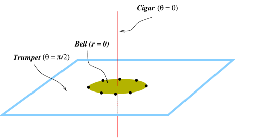
Figure 1: Geometry of the ring of NS5-branes, and sections corresponding to coset CFTs.

It is interesting to look at certain two-dimensional sections, which have a geometry coinciding with gauged $SU(2)/U(1)$ or $SL(2,\mathbb{R})/U(1)$ models (see figure 1):

• $x^{8}=x^{9}=0$ plane, inside of the NS5 circle: the bell

  This section is obtained by taking $r=0$ (see (10)), and the two dimensional slice is a bell

  $$ds^{2}=\alpha^{\prime}k\,[d\theta^{2}+\tan^{2}\theta d\psi^{2}]\,,$$ (14)

  which corresponds to a $SU(2)/U(1)$ WZW model. The singularity at $\theta=\pi/2$ corresponds to the locus of the ring of five-branes. More generically, each slice of the geometry for fixed $r$ can be viewed as a current-current deformation of $SU(2)$ of parameter $\tanh r$ (see also [19, 20]).

• $x^{8}=x^{9}=0$ plane, outside of the NS5 circle: the trumpet

  This section is obtained by taking $\theta=\pi/2$, and the two dimensional slice is the trumpet

  $$ds^{2}=\alpha^{\prime}k\,[dr^{2}+\frac{1}{\tanh^{2}r}d\psi^{2}]\,,$$ (15)

  which corresponds to a vector coset $SL(2,\mathbb{R})/U(1)$ model. Again, the singularity at $r=0$ corresponds to the locus of the ring of fivebranes.

• $x^{6}=x^{7}=0$ plane: the cigar

  This section is obtained by taking $\theta=0$, and the four-dimensional metric is reduced to the cigar

  $$ds^{2}=\alpha^{\prime}k\,[dr^{2}+\tanh^{2}rd\phi^{2}]\,,$$ (16)

  which corresponds to an axial coset $SL(2,\mathbb{R})/U(1)$ model.

Focusing in these two-dimensional sub-manifolds will be useful when we study the shape of D-branes in the NS5 background.

2.1 Two T-dual descriptions of the circle of NS5 branes

Another connection with coset models appears when performing T-duality along the isometries of the background (12) in the directions of $\psi$ and $\phi$.

The T_ψ-dual geometry

After a T-duality along the direction $\psi$ we obtain the dual torsionless solution (fig. 2):

$$ds^{2} = \alpha^{\prime}k\left[dr^{2}+\tanh^{2}r\,\left(\frac{d\chi}{k}\right)^{2}+d\theta^{2}+\mathrm{cotan}^{2}\theta\,\left(\frac{d\chi}{k}-d\phi\right)^{2}\right],$$

$$e^{2\Phi} = \frac{g^{2}_{\textsc{eff}}}{k}\ \frac{1}{\cosh^{2}r\ \sin^{2}\theta}$$ (17)

where $\chi$ is the coordinate T-dual to $\psi$. The background is nothing but a vector $\mathbb{Z}_{k}$ orbifold of the coset theories $SU(2)_{k}/U(1)\,\times SL(2,\mathbb{R})_{k}/U(1)$, i.e. the cigar times T-bell background.

Figure 2: Geometry of the brane setup and T_ψ-duality.

The T_ϕ-dual geometry

A T duality along $\phi$ in (12) yields [21, 20]:

$$ds^{2} = \alpha^{\prime}k\left[dr^{2}+d\theta^{2}+\tan^{2}\theta\left(\frac{d\omega}{k}\right)^{2}+\coth^{2}r\left(\frac{d\omega}{k}+d\psi\right)^{2}\right]$$

$$e^{2\Phi} = \frac{g^{2}_{\textsc{eff}}}{k}\ \frac{1}{\sinh^{2}r\ \cos^{2}\theta}$$ (18)

where $\omega$ is the coordinate dual to $\phi$ and we have written only the non-trivial directions. This is a $\mathbb{Z}_{k}$ orbifold of the vector coset $SU(2)/U(1)$ (the bell) and the vector coset $SL(2,\mathbb{R})/U(1)\$, the trumpet.

These T_ψ,ϕ duals will be the backgrounds in which we start out our construction of the branes. In a second stage, we will re-interpret them in the original NS5 geometry. We note at this point that when we consider supersymmetric branes of even/odd space-dimension in the presence of NS5-branes, we will work in type IIA/B string theory, and the T-dual coset conformal field theory will be a background of type IIB/A string theory.

To study these branes, it is useful to recall properties of the D-branes in the coset backgrounds, which we will use as building blocks for the branes in the background T-dual to the doubly scaled little string theory.

3 Semi-classical description of D-branes

We wish to obtain classical solutions of the Dirac-Born-Infeld action for D-branes in NS5-brane backgrounds. We will concentrate on D-branes that can be constructed out of D-branes of the coset theories $SL(2,\mathbb{R})/U(1)\$and $SU(2)/U(1)$. Indeed the exact boundary states in these gauged WZW theories are known and can be used to construct non-trivial boundary states in the NS5-brane background. This will be the purpose of the following sections. To that end, we will first review the D-branes in the coset models and make some comments. Then we will move to the D-branes in the background of five-branes obtained by T-duality.

3.1 The geometry of D-branes in coset models: a review

As a warm up exercise we review the D-brane taxonomy in the axial and vector cosets $SL(2,\mathbb{R})_{k}/U(1)$ – the cigar and the trumpet – and the axial and vector cosets $SU(2)_{k}/U(1)$ – the T-bell and the bell (see e.g. [22][23]). We consider the following parameterizations of the cigar, the trumpet, the bell and the T-bell respectively:

$$ds^{2}_{c} = k(dr^{2}+\tanh^{2}r\ d\psi_{c}^{2})\qquad e^{\Phi}=\frac{e^{\Phi_{0}}}{\cosh r}$$

$$ds^{2}_{t} = k(dr^{2}+\mbox{cotanh}^{2}r\ d\psi_{t}^{2})\qquad e^{\Phi}=\frac{e^{\Phi_{0}}}{\sinh r}$$

$$ds^{2}_{b} = k(d\theta^{2}+\tan^{2}\theta\ d\psi_{b}^{2})\qquad e^{\Phi}=\frac{e^{\Phi_{0}}}{\cos\theta}$$

$$ds^{2}_{T} = k(d\theta^{2}+\mbox{cotan}^{2}\,\theta\ d\psi_{T}^{2})\qquad e^{\Phi}=\frac{e^{\Phi_{0}}}{\sin\theta}.$$ (19)

with $\psi_{*}\in[0,2\pi)$ and $\theta\in[0,\pi/2]$. We note that the bell and the T-bell allow for an identical geometrical interpretation, i.e. the $SU(2)/U(1)$ coset is geometrically self-dual. We wish to study the D-brane Born-Infeld action in these backgrounds:

$$S_{\textsc{dbi}} = \tau_{p}\int d\xi^{\alpha}e^{-\Phi}\sqrt{-det(g+B+2\pi F)}+S_{WZ},$$ (20)

where $g$ is the induced word-volume metric, $B$ is the induced NS-NS two-form, and $F$ is the world-volume gauge field.

We will always study static branes in the following and we choose static gauge for the time-coordinate: $\xi^{0}=x^{0}$ (i.e. worldsheet time coincides, parametrically, with space-time time). We suppose that the time-direction which is external to the cosets is flat. To parameterize the worldsheet actions, another coordinate system is sometimes convenient, namely:

$$u = \sinh r\ \text{(cigar)},\qquad u=\cosh r\ \text{(trumpet)},\qquad z=\sin\theta\ \text{(bell)},\qquad z=\cos\theta\ \text{(T-bell)}$$

$$ds^{2}_{c} = k\frac{du^{2}+u^{2}d\psi^{2}}{1+u^{2}}\qquad e^{\Phi}=e^{\Phi_{0}}(1+u^{2})^{-1/2}$$

$$ds^{2}_{t} = k\frac{du^{2}+u^{2}d\psi^{2}}{u^{2}-1}\qquad e^{\Phi}=e^{\Phi_{0}}(u^{2}-1)^{-1/2}$$

$$ds^{2}_{b,T} = k\frac{dz^{2}+z^{2}d\psi^{2}}{1-z^{2}}\qquad e^{\Phi}=e^{\Phi_{0}}(1-z^{2})^{-1/2}.$$ (21)

Thus we see that the cigar is conformal to the plane, the bell and the T-bell (which are the same since the background is self-dual) are conformal to the unit disc and the trumpet is conformal to the complement of the unit disc.

Static D0-branes

Static D0-branes in the cigar have an action proportional to:

$$S_{c} \propto \int dt\cosh r$$ (22)

in other words, the D0-branes are only stable at the tip of the cigar. Similarly it can be found that the static D0-brane needs to live at the $r\rightarrow 0$ singularity of the trumpet, at the boundary $\theta\to\pi/2$ of the bell, and also at the boundary $\theta\to 0$ of the T-bell.

Static D1-branes

For static D1-branes we use the alternative coordinate system, and we find the actions:

$$S_{c,t} \propto \int d\xi^{1}\sqrt{u_{\xi^{1}}^{2}+u^{2}\psi^{2}_{\xi^{1}}}$$

$$S_{b,T} \propto \int d\xi^{1}\sqrt{z_{\xi^{1}}^{2}+z^{2}\psi^{2}_{\xi^{1}}}$$ (23)

for branes in the non-compact or compact coset respectively. (We denoted with an lower index $\xi_{1}$ the derivation with respect to $\xi_{1}$.) Thus, the static D1-branes see a flat metric in these coordinates. They are straight lines in the plane with polar coordinates $(u,\psi)$ or $(z,\psi)$. In the original variables, these straight lines (or line segments, or unions of half-lines) are parameterized as:

$$\sinh r\sin(\psi_{c}-\psi_{c}^{0}) = c_{c}$$

$$\cosh r\sin(\psi_{t}-\psi_{t}^{0}) = c_{t}$$

$$\sin\theta\sin(\psi_{b}-\psi_{b}^{0}) = c_{b}$$

$$\cos\theta\sin(\psi_{T}-\psi_{T}^{0}) = c_{T}.$$ (24)

The geometrical interpretation of the D1-brane solutions in all instances is clear. On the one hand, they try to follow a geodesic, to minimize their tensional energy, but on the other hand, they prefer to pass through a regime with strong coupling (i.e. large dilaton) to reduce the tension itself. In the $u,z$ coordinates, the two tendencies of the D1-branes are neatly encoded: the delicate balance is such that the D1-branes follow straight lines in these auxiliary planes. Classically, we can fix their trajectories by specifying (e.g.) their direction at infinity, and their point of nearest approach to the center of the plane.

The seemingly flat behavior of these D1-branes has been exploited in the Lorentzian context of black holes and cosmological singularities in [24][25]. Indeed, those applications clearly illustrate that when the time-direction is curved, we need to revisit our intuitive picture for D-brane dynamics. We continue with a flat time direction in the following.

Static D2-branes

A usual route for the D2-branes would involve fixing the gauge such that space-time and worldvolume coordinates entirely coincide. We choose not to do so, because that gauge choice makes T-duality between D1-branes and D2-branes less manifest, and we wish to prepare ourselves for more involved T-dualities to be performed later. To that end, we choose our gauge as follows: $\xi^{0}=x^{0}$ and $\xi^{2}=\psi_{c,t,b,T}$, while we leave $\xi^{1}$ unfixed. After a brief computation, we find the actions:

$$S_{c,t} \propto \int d\psi d\xi^{1}\ \sqrt{u_{\xi^{1}}^{2}+u^{2}(\frac{2\pi}{k}F_{\psi\xi^{1}})^{2}}$$

$$S_{b,T} \propto \int d\psi d\xi^{1}\ \sqrt{z_{\xi^{1}}^{2}+z^{2}(\frac{2\pi}{k}F_{\psi\xi^{1}})^{2}}.$$ (25)

Since we wish to relate this D2 branes with D1 branes of the T-dual geometries, we have used $u,z$ in their T-dual form, i.e., in the cigar $u=\cosh r_{c}$, in the bell $z=\cos\theta$, etc. We thus see that the actions (25) go under T-duality along $\psi$ to the D1 actions (23) of the T-dual geometries.

The D2 on the cigar and its dual

Let us discuss some of the solutions of the actions in a little more detail in particular instances. The solution to the equations of motion for the cigar can be written as follows:

$$A=\frac{k}{2\pi}\ \left[A_{0}-\arcsin\left(\frac{c}{\cosh r}\right)\right]d\psi,$$ (26)

which allows us to identify the gauge field $A_{\psi}$ on the D2-brane in the cigar with the $\psi_{t}$ coordinate of the D1-brane in the trumpet. Both $c$ and $A_{0}$ are integration constants. We will discuss first the solution with $c<1$. The magnetic field strength on the D2-brane is:

$$F = \frac{k}{2\pi}\left\{[A_{0}-\arcsin(c)]\delta(r)+\frac{c\tanh r}{\sqrt{\cosh^{2}r-c^{2}}}\right\}\ dr\wedge d\psi.$$ (27)

The delta-function contribution can be identified by using Stokes-theorem for a Wilson loop encircling the tip of the cigar. Thus we see that we obtain a delta-function contribution to the origin from the vortex-form for the gauge field, unless we put

$$A_{0} = \arcsin(c).$$ (28)

Note that near the tip of the cigar, the space-time approximates flat space. In flat space, D0-brane flux spreads on a D2-brane worldvolume, to form a bound state. Thus, the concentration of D0-brane charge near the tip is energetically disfavored. To find the minimal energy solution in a given super-selection sector (set by the total magnetic charge) we thus fix the Wilson line such that the magnetic field is non-singular at the origin $A_{0}=\arcsin(c)$. The integral of the magnetic field on the D2-brane wrapping the cigar is then:

$$\frac{1}{2\pi}\int_{cigar}F = \frac{k}{2\pi}\arcsin(c).$$ (29)

Because this flux is responsible for a D0-brane charge, it is likely to be quantized. Indeed a quantization of the parameter $\sigma=\arcsin(c)$ will be needed to interpret the result in the context of the five-branes background. The D0-brane magnetic flux tends to spread near the origin, as in flat space, but at larger distances the flux (as an isolated D0-brane does) tends towards stronger coupling. This leads to a local maximum for the magnetic field at a particular radius ($\sinh^{2}r=\sqrt{1-c^{2}}$). We can discuss the dynamics that leads to these particular static solutions in some more detail. Note that D2-branes covering the whole cigar (which have $|c|<1$) are T-dual to D1-branes in the trumpet background which bump into the disc cut out from the $(u,\psi_{t})$ plane (because of the identification $u=\cosh r$), in other words, they are dual to the D1-branes that reach the open, strongly coupled end of the trumpet.

Finally, note that the topologically trivial Wilson line in the D2-brane reaching the tip of the cigar turns out not to be a zero-mode. By T-duality, the angular position of the D1-brane in the trumpet model is not a true zero-mode. This is familiar. Indeed, we know that the naive isometry in the trumpet is broken in the quantum theory, and that similarly, the winding number is not a fully conserved quantum number in the cigar. Thus, indeed, the fact that the angular variable of the D1-brane in the trumpet is not a true zero-mode is consistent with the known symmetry-breaking patterns of the coset models.

To further discuss the T-duality, let us start with a D2-brane of the cigar with $c<1$, with a gauge field given by eq. (26). To avoid the vortex-like singularity at the origin, we choose $A_{0}=\arcsin(c)=\sigma$. By T-duality of the cigar, we obtain the following $\mathbb{Z}_{k}$ orbifold of the trumpet:

$$ds^{2}=k\left[dr^{2}+\text{cotanh}^{2}\,r\left(\frac{d\tilde{\psi}}{k}\right)^{2}\right]$$ (30)

with the identification $\tilde{\psi}\sim\tilde{\psi}+2\pi$. We have in this background a D1-brane of embedding equation $\sin\sigma=\cosh r\sin(\tilde{\psi}/k-\sigma)$. To recover the standard trumpet CFT – i.e. the vector coset of the single cover of $SL(2,\mathbb{R})\$– one can go to the covering space of the orbifold by defining $\phi=\tilde{\psi}/k$ with the periodicity $\phi\sim\phi+2\pi$. This gives an extra freedom for the D1-brane, corresponding to the copy of the orbifold manifold we start with on the covering space.

To summarize we have argued that for the D1-branes of the trumpet with $c<1$ the angular position has to be quantized as $\psi^{0}_{t}=\arcsin(c)+\frac{2\pi\hat{p}}{k}$, with $\hat{p}\in\mathbb{Z}_{k}$, to be consistent with the T-dual picture. Since the D2-branes of the cigar with $c>1$ do not reach the singularity, the parameter $\psi^{0}_{t}$ of the corresponding D1-branes in the trumpet would not be quantized. By the same reasoning we find that the parameter $\psi^{0}_{c}$ for the D1-branes of the cigar is not quantized, and that for the D1-branes of the bell the parameter $\psi^{0}_{b}$ is quantized as $\psi^{0}_{b}=\theta_{0}+\frac{2\pi\hat{p}}{k}$. The angles corresponding to the two endpoints of the D1-brane on the boundary of the disc are then

$$(\psi_{1},\psi_{2})=\left(\frac{2\pi\hat{p}}{k}+2\theta_{0},\frac{2\pi\hat{p}}{k}+\pi\right)$$ (31)

We will see later that these heuristic rules will get a natural interpretation in the CFT of the ring of fivebranes.

Needless to say, the geometrical picture for the trumpet is known to be corrected drastically by worldsheet instantons and the physics is more truthfully encoded in the sine-Liouville model – we have just used the trumpet to gain geometrical intuition on the D-brane solutions discussed above. However by requiring the consistency of the D-branes profiles with the T-duality we have gained some insight on the quantization of the parameters of the branes, which would properly require to be analyzed using the non-perturbative corrections to the sigma-models. Now, we’ll turn to applying these techniques in more complicated examples.

3.2 D-branes in the NS5-branes background

Now we shall use the T-dual representations of the background of NS5-branes on a circle, i.e. the (orbifold of) the product of coset models, eqs. (17,18) in order to construct a number of non-trivial D-branes in the original NS5-brane background.

In this paper we are mainly interested by stable, BPS D-branes preserving a fraction of supersymmetry. As will become clear in the CFT analysis, we have then to choose, say in the $T_{\psi}$-dual background, the same A- or B-type boundary conditions for both axial cosets, $SL(2,\mathbb{R})/U(1)\$(the cigar) and $SU(2)/U(1)$ (the T-bell). Under this condition the spectrum of open strings ending on one of these D-branes will be supersymmetric, indicating their BPS nature. The supersymmetry of these D-branes could also be checked at the level of the DBI action, using e.g. the techniques of [30].

Suspended D1-branes

These are D1-branes ending on both sides on a NS5-brane in type IIB superstrings. They are of special interest, because they correspond to the “W-bosons” of the Little String Theory, namely the D1-branes stretched between the NS5-branes corresponding to the broken gauge symmetry of the higgsed configuration, that remain massive in the double scaling limit. The D1-branes can be constructed from a D0-brane in the cigar and a D2-brane in the T-bell:

$$r=0\ ,\ \ F=\frac{k}{2\pi}\ \frac{\sin\theta_{0}\,\text{cotan}\,\theta}{\sqrt{\sin^{2}\theta-\sin^{2}\theta_{0}}}\ d\theta\wedge d\chi.$$ (32)

Since the D0-brane of the cigar sits at the tip (and the coordinate $\chi$ plays the role of the angular coordinate on the T-bell at $r=0$), by T-duality we will simply get a D1-brane of the bell embedded in the four-dimensional geometry of the transverse space:

$$\sin\theta\sin(\psi-\psi_{0})=\sin\theta_{0}$$ (33)

These D1-branes are straight lines in the $(x^{6},x^{7})$ plane, using the coordinate transformations (10), ending on the ring of fivebranes. The parameter $\psi_{0}$ becomes quantized once we take into account the T-duality considerations discussed in the previous section or the exact CFT description. The parameter $\theta_{0}$ is also quantized in the exact CFT, and it can be understood by advocating the flux stabilization of the D2-branes in $SU(2)$ [31]. With these quantization rules the D1-branes are then stretched between two NS5-branes out of the $k$ NS5-branes that make up the background – the configuration is discussed in more detail below.

A first D3-brane from T_ψ duality

We are now ready to study a D3-brane in the NS5-brane background. We start in the T_ψ dual background (17) and consider the product of a D1-brane in the cigar times a D1-brane in the T-bell. The equations for the branes are:

$$\sinh r\sin\left(\frac{\chi}{k}-\psi_{0}\right) = \sinh r_{0}\,,$$

$$\cos\theta\sin\left(\frac{\chi}{k}-\phi+\phi_{0}\right) = \cos\theta_{0}\,.$$ (34)

To obtain a D3 brane in the NS5 background, we perform now a T duality along $\chi$. We first solve for the coordinate $\chi$ which by T-duality goes to a dual gauge field as $\chi\rightarrow 2\pi A_{\psi}$. Secondly, we eliminate the coordinate $\chi$ on which we perform T-duality from the equations (34) for the profile of the D3 brane. We obtain:

$$\arcsin\left(\frac{\sinh r_{0}}{\sinh r}\right) = \arcsin\left(\frac{\cos\theta_{0}}{\cos\theta}\right)+\phi-\phi_{0}-\psi_{0}$$ (35)

$$A = \frac{k}{2\pi}\ \left[\arcsin\left(\frac{\sinh r_{0}}{\sinh r}\right)+\psi_{0}\right]d\psi\,,$$

$$= \frac{k}{2\pi}\ \left[\arcsin\left(\frac{\cos\theta_{0}}{\cos\theta}\right)+\phi-\phi_{0}\right]d\psi\,.$$

The profile of the T-dual D3-brane is thus highly non-trivial and non-factorized. The two expressions (3.2) for the gauge field are related by the embedding equation (35).

The D3 brane worldvolume wraps the $\psi$ coordinate in (12), times a two-dimensional manifold defined by the constraint (35) in the $(r,\theta,\phi)$ coordinates. This two-dimensional manifold can be interpreted as straight lines in the $(\sinh r,\phi)$ plane, which are shifted and tilted as a function of $\theta$:

$$\sinh r_{0}\cos\theta = \sinh r\left[\cos\theta_{0}\cos(\phi-\phi_{0}-\psi_{0})+\sqrt{\cos^{2}\theta-\cos^{2}\theta_{0}}\sin(\phi-\phi_{0}-\psi_{0})\right],$$

and the gauge field gives the following magnetic field:

$$F = \frac{k}{2\pi}\,\frac{\text{cotanh}\,r}{\sqrt{\frac{\sinh^{2}r}{\sinh^{2}r_{0}}-1}}\ \ d\psi\wedge dr\,,$$ (38)

$$= \frac{k}{2\pi}\left[d\phi\wedge d\psi+\frac{\tan\theta}{\sqrt{\frac{\cos^{2}\theta}{\cos^{2}\theta_{0}}-1}}\ d\theta\wedge d\psi\right].$$ (39)

Note that while the parameter $\phi_{0}$ is quantized (see above), the parameter $\psi_{0}$ is not; so we can absorb the former by shifting the latter. The gauge for the B-field that is consistent with this expression for the magnetic field is implicitly fixed by the particular T-duality we have chosen to construct the D-branes. The worldvolume of this D-brane is restricted to:

$$r>r_{0}\ ,\ \ \theta<\theta_{0}.$$ (40)

In view of the non-trivial nature of the solution, it is instructive to directly check that it is a solution, using the D3-brane Dirac-Born-Infeld action in the NS5-brane background. That is a non-trivial exercise which we performed following the general ideas in [26]. In this way it is clearly possible to construct highly non-trivial D3-brane configurations in the NS5-brane geometry.

Limit profiles

To understand in more detail the profile of this D3-branes we can go to some particular limits of the bulk coordinates or the D-brane parameters:

• in the limit $\theta\to 0$ we focus on the two-plane defined by $x^{6}=x^{7}=0$ (see e.g. 10). As we saw in section 2 the transverse space metric degenerates to the cigar corresponding to coordinates $(r,\phi)$. Then the equation defining the D3-brane becomes simply $\sinh r_{0}=\sinh r\cos(\phi-\phi_{0}-\psi_{0}-\theta_{0})$, i.e. the D1-brane of the cigar. Going back to the Cartesian coordinates for the transverse space, eq (10), they are straight lines defined by: $x^{6}=x^{7}=0$ and $x^{8}=\rho_{0}\sinh r_{0}$. Therefore $r_{0}$ corresponds to the distance of closest approach of these D-branes with respect to the NS5-branes.

• In the limit $r\to\infty$, the metric approaches the solution for coincident NS5-branes, i.e. $\mathbb{R}_{Q}\times SU(2)_{k}$. It is an intermediate regime which is still near horizon but far enough to approximate the configuration with coincident fivebranes. The equation for the D-brane becomes $\cos\theta_{0}=\pm\cos\theta\sin(\phi-\phi_{0}-\psi_{0})$, i.e. a symmetric $S^{2}$ D2-brane of $SU(2)$. Strictly speaking we obtain two antipodal D2-branes corresponding to the two branches of the solution.

• for the D3-brane with parameter $r_{0}=0$, we can take the $r\to 0$ limit to focus on the plane $x^{8}=x^{9}=0$ where the NS5-branes live. The metric then degenerates to the bell $SU(2)/U(1)$, the bell coordinates being $(\theta,\psi)$. The $k$ special points on the boundary of the bell correspond to the position of the five-branes. As the $\phi$ coordinate degenerates, the equation becomes simply $\theta<\theta_{0}$, i.e. a D2-brane of the bell, carrying a gauge field given by the second term of (39)

Note that the parameter $\phi_{0}$ is not quantized, which is consistent with the geometrical fact that the $SO(2)$ rotational isometry in the $(x^{8},x^{9})$ plane is not broken by the distribution of fivebranes. The D2-branes of the coset $SU(2)/U(1)$ can be considered as bound states of D0-branes sitting at the center of the bell [22]. Therefore we can reinterpret this class of D3-branes as a bound state of D1-branes transverse to the NS5-branes, defined by the equations (for $\phi_{0}+\psi_{0}+\theta_{0}=0$):

$$x^{6}=x^{7}=x^{9}=0\ ,\ \ x^{8}=\rho_{0}\sinh r_{0}.$$ (41)

A second class of D3-branes from T_ϕ duality

A second, closely related D3-brane can be constructed by starting from D1 branes in the T_ϕ dual geometry (18). This exchanges the roles of the $SL(2,\mathbb{R})\$$/U(1)$ coset and the $SU(2)/U(1)$ coset by their T-duals.

Explicitly we start from the following D1-branes of the trumpet (the vector $SL(2,\mathbb{R})\$$/U(1)$ coset) and the bell (i.e. the vector $SU(2)/U(1)$ coset):

$$\cosh r\,\sin\left(\frac{\omega}{k}+\psi-\psi_{0}\right) = c$$

$$\sin\theta\sin\left(\frac{\omega}{k}-\phi_{0}\right) = \sin\theta_{0}$$ (42)

It will be useful to distinguish once again the D1-branes with $c>1$ which do not reach the $r=0$ end of the trumpet – we will name them ”uncut” –, and the D1-branes with $c<1$ which reach the end of the trumpet – ”cut”. For each case, we will use the parameterization:

$$c=\cosh r_{0}\ ,\ \ c\geqslant 1\quad\text{and}\quad c=\sin\sigma\ ,\ \ c<1$$ (43)

We revisit this distinguishing characteristic in the exact construction of the boundary states.

Going through the same steps of the T-duality (this time along $\phi$), we find the following non-trivial D3-branes:

$$c\,\sin\theta = \cosh r\left[\sin\theta_{0}\cos(\psi+\phi_{0}-\psi_{0})+\sqrt{\sin^{2}\theta-\sin^{2}\theta_{0}}\sin(\psi+\phi_{0}-\psi_{0})\right],$$

$$F = \frac{k}{2\pi}\ \frac{\text{cotan}\,\theta}{\sqrt{\frac{\sin^{2}\theta}{\sin^{2}\theta_{0}}-1}}\ d\phi\wedge d\theta$$ (44)

$$= \frac{k}{2\pi}\left[d\phi\wedge d\psi+\frac{\tanh r}{\sqrt{\frac{\cosh^{2}r}{c^{2}}-1}}\ d\phi\wedge dr\right]$$

We have a non-trivial magnetic field on the D3-brane. The worldvolume of this D-brane is restricted to:

Uncut: $$\quad r>r_{0}\ ,\ \ \theta>\theta_{0}$$

Cut : $$\quad\theta>\theta_{0}$$

We can as in the previous case consider various limits of the solution.

The uncut branes

• in the limit $\theta\to\pi/2$ we focus on the two-plane defined by $x^{8}=x^{9}=0$, and in the region outside the ring of five-branes, i.e. $x^{6},x^{7}\geq\rho_{0}$. Then (see sect. 2) the metric degenerates to the trumpet, with coordinates $(r,\psi)$. We then get from this class of D3-branes ”uncut” D1-branes of the trumpet of equation $\cosh r_{0}=\cosh r\cos(\psi+\phi_{0}-\psi_{0}-\theta_{0})$.

• In the $r\to\infty$ limit we obtain a D2-brane of $SU(2)$ as for the other kind of D3-branes, but with a different position.

The cut branes

In this case first, as we argued in our discussion of the D-branes in the coset models, the parameter $\psi_{0}$ will be quantized as $\psi_{0}=\sigma+2\pi\hat{p}/k$. Then the picture is modified as follows.

• In the $\theta_{0}=0$ case, in $\theta\to 0$ limit, we get the smooth D2 of the cigar with gauge field strength $2\pi F_{r\phi}=k\sin\sigma\tanh r/\sqrt{\cosh^{2}r-\sin^{2}\sigma}$ getting its maximal value at some finite distance from the tip.

• In the $\theta\to\pi/2$ limit we get an cut D1-brane of the trumpet, of embedding equation: $\sin\sigma=\cosh r\sin(\psi+\phi_{0}-\psi_{0}+\theta_{0})$, with all the parameters quantized. To be precise we get a second copy of this D1-brane rotated by $\pi-2\theta_{0}$.

• in the $r\to\infty$ limit, we get again a D2-brane of $SU(2)$.

• For all these cut branes we can take the $r\to 0$ limit; then we go to the plane defined by $x^{8}=x^{9}=0$, where the metric of the five-branes degenerates to the bell (of coordinates $ds^{2}=d\theta^{2}+\tan^{2}\theta d\psi^{2}$). and we get a D1-brane of the bell (more precisely, again two D1-branes), of embedding equation: $\sin\theta_{0}=\sin\theta\sin(\psi_{0}+\sigma-\phi_{0}-\psi)$. This suggests strongly that the parameter $\sigma$ has to be quantized as well.

Semi-infinite D1-branes

The previous class of D3-branes contains as a special case ”D-rays”, which are semi-infinite D1-branes coming in from infinity. They correspond to D3-branes with parameter $\theta_{0}=\pi/2$. Their worldvolume is thus restricted to $\theta=\pi/2$, corresponding to the plane $x^{8}=x^{9}=0$, but outside the ring of NS5-branes; then the metric degenerates to the trumpet. These D1-branes are given by the embedding equation:

$$\cosh r\cos(\psi+\phi_{0}-\psi_{0})=c$$ (45)

They consist in straight lines in the plane $(x^{6},x^{7})$, in the domain $\sqrt{(x^{6})^{2}+(x^{7})^{2}}>\rho_{0}$ outside the ring. If for example we choose $\phi_{0}-\psi_{0}=0$, the equation for the D1-brane is $x^{6}=c/\rho_{0}$, with the condition $\sqrt{c^{2}+(\nicefrac{{x^{7}}}{{\rho_{0}}})^{2}}>1$.

Let us consider first the case $c<1$, i.e. the ”cut” D-branes. These D-branes are made of two semi-infinite D1-branes ending on the ring. The parameter $\psi_{0}$ is quantized for the ”cut” branes as $\psi_{0}=\sigma+2\pi\hat{p}/k$. Then, if we insist that these D1-branes end on NS5-branes, we have to choose only D-branes with $\sigma\in\pi\mathbb{Z}/k$. This will be confirmed by the CFT analysis. We have obtained a semi-infinite D1-brane that ends on the ring precisely on a specific NS5-brane. The physics of D4-branes T-dual of these D1-branes along $x^{1,2,3}$ has been discussed in [11].

On the contrary the ”uncut” D-branes (i.e. with $c>1$) will give in the NS5-brane background infinite D1-branes avoiding the ring of five-branes entirely. For these infinite D1-branes avoiding the ring of NS5-branes there is no reason for a quantization of $\psi_{0}$. Note finally that this picture will be a little bit modified in the exact CFT analysis, since strictly speaking there is no exact D-brane with $\theta_{0}=\pi/2$. Thus our picture is valid in the semi-classical large $k$ limit, but at finite $k$ the picture is fuzzy, since these D1-branes have some extension in their transverse directions.

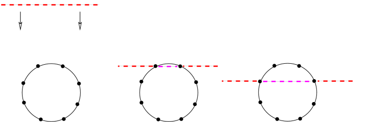
Figure 3: Geometry of a D1-brane for different values of $c$. For $c>1$ (left) the infinite D1-brane avoids the ring of fivebranes and corresponds to an ”uncut” D1 of the trumpet. For $c<1$ (right) the D1-brane intersects the ring; its two semi-infinite halves correspond to a ”cut” D1 of the trumpet and the finite part inside the ring to a D1-brane of the bell.

In the course of our analysis we observe a remarkable phenomenon, see fig. 3. The interior and the exterior of the ring of fivebranes (both in the plane $x^{8}=x^{9}=0$) are both described by exact coset CFTs, respectively the bell $SU(2)/U(1)$ and the trumpet (the vector coset $SL(2,\mathbb{R})/U(1)\$). We can bring D1-branes from infinity (i.e. for $c>1$) to the ring of fivebranes; when the D1-branes intersects the ring of fivebranes they break into two parts: a D1-brane of the trumpet corresponding to the two semi-infinite halves of the D-string outside the ring – and ending on NS5branes – and a D1-brane of the bell corresponding to the finite D1-branes suspended between the NS5-branes. Thus we have an exact CFT realization of the configurations discussed in [16], in which a D-brane can split into two halves when it crosses a NS5-brane.

In this section, we used the geometrical picture for branes in coset models to construct non-trivial branes in the NS5-brane background. The T-duality involved in developing the correct geometrical picture was often intricate. We have considered all the combinations of coset branes in the T-dual picture that would lead to BPS D-branes in the background of fivebranes. It would be worthwhile to examine the set of semi-classical brane profiles that cannot be obtained using the techniques explained in this section, i.e. that cannot be expressed in the T-dual geometry as product of D-branes of $SL(2,\mathbb{R})/U(1)\$and $SU(2)/U(1)$. We now turn to constructing the exact boundary states corresponding to the branes we discussed.

4 Exact construction of branes

To construct branes consistent with the bulk theory, it is useful to recall the spectrum of closed strings in the bulk – the cylinder amplitude in the doubly scaled little string theory background will need to be consistent with the bulk spectrum obtained from the torus partition function. For simplicity, we mostly work with branes in type IIB theory. D-branes of type IIA are obtained by an odd number of T-dualities along the flat directions $x^{1,2,3,4,5}$.

Bulk spectrum

The most non-trivial feature in the spacetime-supersymmetric spectrum of the type II doubly scaled little string theory is the spectrum of the $SL(2,\mathbb{R})/U(1)$ superconformal field theory [32][33][9]. In the full NS5-brane background it leads to the identification of the discrete spectrum, built with the discrete representations of $SL(2,\mathbb{R})_{k}$ of spin $j$, together with representations of $SU(2)_{k}$ of spin $j^{\prime}$:

$$Z_{d}=\frac{1}{2}\sum_{a,b\in\mathbb{Z}_{2}}(-)^{a+b}\ \frac{1}{2}\sum_{\bar{a},\bar{b}\in\mathbb{Z}_{2}}(-)^{\bar{a}+\bar{b}+\varepsilon\bar{a}\bar{b}}\frac{\vartheta^{2}{a\atopwithdelims[ ]b}\bar{\vartheta}^{2}{\bar{a}\atopwithdelims[ ]\bar{b}}}{(8\pi^{2}\tau_{2})^{2}\eta^{4}\bar{\eta}^{4}}\ \sum_{2j^{\prime}=0}^{k-2}\sum_{2j=1}^{k+1}\Upsilon(2j,1)\sum_{m,\bar{m}\in\mathbb{Z}_{2k}}\sum_{w_{L},w_{R}\in\mathbb{Z}}$$

$$\mathcal{C}^{j^{\prime}}_{m}{a\atopwithdelims[ ]b}\bar{\mathcal{C}}^{j^{\prime}}_{-\bar{m}}{\bar{a}\atopwithdelims[ ]\bar{b}}ch_{d}(j,\frac{m}{2}+kw_{L}-j-\frac{a}{2}){a\atopwithdelims[ ]b}ch_{d}(j,-\frac{\bar{m}}{2}+kw_{R}-j-\frac{\bar{a}}{2}){\bar{a}\atopwithdelims[ ]\bar{b}}$$

where $\varepsilon=0$ in type IIB superstrings and $\varepsilon=1$ in type IIA. We have also defined $\Upsilon(2j,1)=\nicefrac{{1}}{{2}}$ if $2j=1\mod k$, $\Upsilon(2j,1)=1$ otherwise.

This expression involves the characters $\mathcal{C}^{j}_{m}{a\atopwithdelims[ ]b}$ of the N=2 minimal models and the discrete characters $ch_{d}(j,r){a\atopwithdelims[ ]b}$ of $SL(2,\mathbb{R})/U(1)$ (see appendix A), associated to the non-flat coset factors $SU(2)/U(1)$ and $SL(2,\mathbb{R})/U(1)$ respectively. The sum over left and right winding separately is necessary to allow for the twisted sectors of the orbifolded cosets. Note that this partition function is obtained by performing first a $\mathbb{Z}_{k}$ diagonal orbifold of the product of the two cosets $SU(2)_{k}/U(1)$ and $SL(2,\mathbb{R})_{k}/U(1)$, and then a specific $\mathbb{Z}_{2}$ projection to obtain odd-integral $N=2$ charges, see [33] [9] for details.

Then we have a continuous spectrum constructed with the continuous representations of $SL(2,\mathbb{R})$, of spin $j=1/2+iP$:

$$Z_{c}=\frac{1}{2}\sum_{a,b\in\mathbb{Z}_{2}}(-)^{a+b}\frac{1}{2}\sum_{\bar{a},\bar{b}\in\mathbb{Z}_{2}}(-)^{\bar{a}+\bar{b}+\varepsilon\bar{a}\bar{b}}\frac{\vartheta^{2}{a\atopwithdelims[ ]b}\bar{\vartheta}^{2}{\bar{a}\atopwithdelims[ ]\bar{b}}}{(8\pi^{2}\tau_{2})^{2}\eta^{4}\bar{\eta}^{4}}\ \sum_{2j^{\prime}=0}^{k-2}\ \sum_{m,\bar{m}\in\mathbb{Z}_{2k}}\mathcal{C}^{j^{\prime}}_{m}{a\atopwithdelims[ ]b}\bar{\mathcal{C}}^{j^{\prime}}_{-\bar{m}}{\bar{a}\atopwithdelims[ ]\bar{b}}$$

$$\int_{0}^{\infty}dP\sum_{w_{L},w_{R}\in\mathbb{Z}}\rho(P,m+2kw_{L},-\bar{m}+2kw_{R};a,\bar{a})\phantom{aaaaaaaaaaaaaaaaaaaa}$$

$$ch_{c}(P,\frac{m}{2}+kw_{L}){a\atopwithdelims[ ]b}ch_{c}(P,-\frac{\bar{m}}{2}+kw_{R}){\bar{a}\atopwithdelims[ ]\bar{b}}$$

(47)

The $SL(2,\mathbb{R})/U(1)$ part, written with continuous characters, involves a non-trivial density of states $\rho$ which consists of a term proportional to the infinite volume and a regulator dependent sub-leading term which is the derivative of the phase-shift of the regularizing potential [33][9]. In both cases we denote the primary operators of the doubly scaled LST background as, for states in the NS vacuum:

$$V_{j^{\prime}m\bar{m}\ jw_{L}w_{R},{\bf p}}=e^{-\phi-\tilde{\phi}}\ e^{i{\bf p\cdot X}}\Phi^{SU(2)/U(1)}_{j^{\prime},\ m,\ -\bar{m}}\widetilde{\Phi}^{SL(2,R)/U(1)}_{j,\ \frac{m}{2}+kw_{L},\ -\frac{\bar{m}}{2}+kw_{R}}~{},$$ (48)

where the first factor corresponds to the bosonized NS-NS ground state of the super-reparameterization ghosts. In general the operators carry fermionic labels. For convenience, we will use in the following the formalism in which the fermions are bosonized to a compact $U(1)_{2}$ boson, at level $2$ which carries $\mathbb{Z}_{4}$ valued chiral momenta, as explained in appendix A.

To orient the reader and fix our conventions, we recall that the non-trivial part of the two-point function for two NS-NS primaries is given by:

$$\langle V_{j^{\prime}m\bar{m}\ jw_{L}w_{R},{\bf p}}V_{\tilde{j}^{\prime}\tilde{m}\tilde{\bar{m}}\ \tilde{j}\tilde{w}_{L}\tilde{w}_{R}{\bf p^{\prime}}}\rangle\sim\delta^{(6)}({\bf p}-{\bf p^{\prime}})\,\delta_{j^{\prime},\tilde{j}^{\prime}}\,\delta_{m,\tilde{m}}\,\delta_{\bar{m},\tilde{\bar{m}}}\,\delta_{w_{L},\tilde{w}_{L}}\delta_{w_{R},\tilde{w}_{R}}$$

$$\times\ \left[\delta(j+\tilde{j}+1)+R(j,\frac{m}{2}+kw_{L},-\frac{\bar{m}}{2}+kw_{R})\delta(j-\tilde{j})\right]\,,$$

in terms of the reflection coefficient:

$$R\left(j,\frac{m}{2}+kw_{L},-\frac{\bar{m}}{2}+kw_{R}\right)=\phantom{aaaaaaaaaaaaaaaaaaaaaaaaaaaaaaaaaaaaaaaaaa}$$

$$\nu_{k}^{\frac{1}{2}-j}\frac{\Gamma(1-2j)}{\Gamma(2j-1)}\frac{\Gamma(j+\frac{m}{2}+kw_{L})\Gamma(j+\frac{\bar{m}}{2}-kw_{R})}{\Gamma(1-j+\frac{m}{2}+kw_{L})\Gamma(1-j+\frac{\bar{m}}{2}-kw_{R})}\frac{\Gamma(1+\frac{1-2j}{k})}{\Gamma(1-\frac{1-2j}{k})}\qquad$$ (49)

with $\nu_{k}=\Gamma(1-\nicefrac{{1}}{{k}})/\Gamma(1+\nicefrac{{1}}{{k}})$.

We recalled a few aspects of the bulk theory, and we now wish to analyze the introduction of boundaries in the worldsheet conformal field theory, i.e. we will construct examples of D-branes, and their corresponding one-point function. In this exact analysis we roughly follow the scheme we set out in the previous section, where the semi-classical behavior of these D-branes was analyzed. It will be useful to keep the semi-classical pictures in mind while analyzing the exact boundary states.

4.1 Boundary states for suspended D1-branes

Let us now construct the exact D1-branes consistent with the closed string theory reviewed above. We are considering first the D1 branes, or W-bosons, stretched between the NS5 branes of which we analyzed the semi-classical behavior in subsection 3.2. We take the NS5-branes and the D1-branes to span the following directions (schematically):

$$\begin{array}[]{c|cccccccccc}&0&1&2&3&4&5&6&7&8&9\\ \hline\cr\text{NS5}&/\hskip-2.84526pt/&/\hskip-2.84526pt/&/\hskip-2.84526pt/&/\hskip-2.84526pt/&/\hskip-2.84526pt/&/\hskip-2.84526pt/&\perp&\perp&\perp&\perp\\ \text{D1}&/\hskip-2.84526pt/&\perp&\perp&\perp&\perp&\perp&/\hskip-2.84526pt/&\perp&\perp&\perp\\ \end{array}\\$$

In that case, as explained is section 3, the D1-brane geometries are factorisable in terms of coset branes and the T-duality acts straightforwardly on them. The D1-branes consist of a product of D1-branes of the N=2 minimal model (i.e. the coset $SU(2)/U(1)$) and the D0-brane of the cigar. We refer to fig. 4) for a drawing of the geometry.

Figure 4: Geometry of the D1-branes and their T-duals.

The D1-branes in the N=2 minimal model are straight lines connecting the $k$ special points on the boundary corresponding to the localization of the NS5-branes. The positions will be labeled by $\hat{n}$ which indicates the middle point of the brane on the boundary of the disc, and the Cardy label $\hat{\jmath}$ giving the angle spanned by the whole D1-brane. Indeed the D1-branes is extended between the angles(see [22]):

$$\psi_{1}=\frac{\pi(\hat{n}-2\hat{\jmath}-1)}{k}\ \ \text{and}\ \ \psi_{2}=\frac{\pi(\hat{n}+2\hat{\jmath}+1)}{k}$$ (50)

Thus (up to a rotation of $\pi$) these labels are related to the labels discussed in sect. 3.1 as follows, see eq. (31):

$$\frac{\pi}{2}-\theta_{0}=\frac{\pi(2\hat{\jmath}+1)}{k}\ \ \text{and}\ \ \hat{p}=\frac{\hat{n}+2\hat{\jmath}+\hat{s}}{2}$$ (51)

with $2\hat{\jmath}=0,1,\ldots,k-2$ and $\hat{n}\in\mathbb{Z}_{2k}$. Note that $\hat{p}$ is indeed integer, thanks to the selection rule (110). There is an overall rotation of the picture by $\pi/k$ depending on the parity of $\hat{s}$. However, since D-branes with values of $\hat{s}$ of different parities cannot appear simultaneously (see appendix B), it doesn’t alter the geometrical interpretation of the branes. These fermionic Cardy labels $\hat{s}_{i}$ for $i=1,2,3,4$ indicate the particular boundary conditions or the projections performed on the worldsheet fermions.

The D0-branes of the cigar (i.e. $SL(2,\mathbb{R})/U(1)$) are point-like objects sitting at the tip, with only a fermionic label, which we will take to correspond to $\hat{s}_{4}$. They have been obtained in [14, 34, 35]. In the NS5-branes geometry, the fact that the D0-brane of the cigar lives at its tip is interpreted as the fact that the D1-branes stretched between the NS5-branes are localized on the two-planes in which the fivebranes live.

The one-point function

Now that we have a reasonable idea of what kind of labels to expect for our boundary states, we turn to the exact expression for the one-point function. We will work in the following in the light-cone gauge. As explained in [36, 37] we put Dirichlet boundary conditions on the lightcone directions. Moreover, in the directions transverse to the NS5-brane the D-branes are of type A in the minimal model directions and of type B in the remaining two directions (where we use the nomenclature of type A and B as applying to factor conformal field theories, and not to the whole of the D-brane). An analysis of the relation between type A/B branes and Neumann and Dirichlet boundary conditions (as the one summarized in appendix B for branes in flat type II superstrings) then teaches us that in the remaining four directions of the worldvolume of the NS5-branes, the boundary conditions can be chosen to be of type A (label $\hat{s}_{1}$) for the coordinates $(x^{2},x^{3})$ and type B (label $\hat{s}_{2}$) for the directions $(x^{4},x^{5})$. After Wick rotation back to ordinary Minkowski space, this allows for the $1+1$ dimensional worldvolume of the D-string.

By combining the known one-point function for the branes for a free scalar, the $N=2$ minimal model, and the $N=2$ non-compact conformal field theories, and implementing the orbifold procedure on these one-point functions, we obtain the following one point-function for the W-bosons of Little String Theory (i.e. the suspended D1-branes):

$$\langle\ V_{j^{\prime}m\bar{m}jw_{L}w_{R},{\bf p}}^{(s_{i})\ (\bar{s}_{i})}\ \rangle^{\textsc{w}}_{\hat{\jmath},\hat{n},\hat{s}_{i},{\bf\hat{y}}}=\frac{\nu_{k}^{\frac{1}{2}-j}\phantom{\!\!\!\!\!}}{k}\ \ \delta_{m,\bar{m}}\delta_{m+2kw_{L},\bar{m}-2kw_{R}}\ \delta_{s_{1},\bar{s_{1}}}\delta_{s_{2},-\bar{s_{2}}}\delta_{s_{3},\bar{s_{3}}}\delta_{s_{4},-\bar{s_{4}}}\,\delta(p^{5})$$

$$e^{i\sum_{i=0}^{4}p^{i}\hat{y}^{i}}e^{i\frac{\pi}{2}\sum_{i}s_{i}\hat{s}_{i}}\ e^{-i\pi\frac{m\hat{n}}{k}}\ \frac{\sin\pi\frac{(1+2j^{\prime})(1+2\hat{\jmath})}{k}}{\sqrt{\sin\pi\frac{1+2j^{\prime}}{k}}}\ \frac{\Gamma\left(j+\frac{m-s_{4}}{2}+kw\right)\Gamma\left(j-\frac{m-s_{4}}{2}-kw\right)}{\Gamma(2j-1)\Gamma(1-\frac{1-2j}{k})}.$$

(52)

On the left hand side, we have labels for the primary field of the minimal model, with given spin and left and right momentum, and likewise for the primary of the non-compact $N=2$ model. Moreover the labels $s_{i}$ and $\bar{s}_{i}$ indicate the chiral momenta of the bosonized pairs of fermions. The lower indices are the (generalized) Cardy labels of the boundary state. In the right hand side, we have substituted $w=w_{L}=-w_{R}$ (which follows from the constraints on the quantum numbers to have a non-trivial one-point function). We have moreover explicitly denoted the flat space one-point functions, which are well-known. This expression is valid both for continuous representations, $j=1/2+iP$, and for the discrete ones with $j$ real. Indeed, the one-point function has poles for the discrete representations, which correspond to couplings with states localized on the NS5-branes plane (no poles arise due to the infinite volume of the non-compact $N=2$ theory, since the D0-brane is a localized object). The couplings to these discrete representations are then given by the residues at the poles. We perform a Cardy-type consistency check on this one-point function next.

The open string partition function

We start with the following integrand for the annulus amplitude for open strings stretched between two D1-branes of the doubly scaled LST:

$$Z^{\textsc{w}}_{\text{open}}=\sqrt{-i\tau}\ \frac{q^{\frac{1}{2}\left(\frac{\bf\hat{y}-\hat{y}^{\prime}}{2\pi}\right)^{2}}}{\eta(\tau)^{4}}\sum_{\{\upsilon_{i}\}\in(\mathbb{Z}_{2})^{4}}\frac{1}{2}\sum_{a,b=0}^{1}(-)^{b}(-)^{a(1+\sum_{i}\upsilon_{i})}\chi^{(b+2\upsilon_{1}+\hat{s}_{1}^{\prime}-\hat{s}_{1})}\chi^{(b+2\upsilon_{2}+\hat{s}_{2}^{\prime}-\hat{s}_{2})}$$

$$\sum_{2j=0}^{k-2}\sum_{n\in\mathbb{Z}_{k}}N^{j}_{\hat{\jmath}\ \hat{\jmath\,}^{\prime}}\ \mathcal{C}^{j\ (b+2\upsilon_{3}+\hat{s}_{3}^{\prime}-\hat{s}_{3})}_{2n+b+\hat{n}-\hat{n}^{\prime}}(\tau)\ Ch_{\mathbb{I}}^{(b+2\upsilon_{4}+\hat{s}_{3}^{\prime}-\hat{s}_{3})}(n;\tau),$$

(53)

written in terms of the $SU(2)_{k-2}$ fusion rules (see appendix A), given through the Verlinde formula in term of the modular S-matrix: $N^{j}_{\hat{\jmath}\ \hat{\jmath\,}^{\prime}}=\sum_{j^{\prime}}S^{\hat{\jmath}}_{\ j^{\prime}}S^{\hat{\jmath\,}^{\prime}}_{\ j^{\prime}}S^{j}_{\ j^{\prime}}/S^{0}_{\ j^{\prime}}$. The $SL(2,\mathbb{R})/U(1)$ factor corresponds to the character of the identity representation, see appendix A. Note that the discrete momentum takes even values in the NS sector and odd values in the R sector. An similar open string partition function has been found in [14], using modular bootstrap techniques. We discuss it in slightly more detail here in view of its importance for Little String Theory.

Our goal is to show that this (physically sensible) open string spectrum is consistent with the one-point function recorded above. As in flat space, the labels $\hat{s}_{i}$ of the branes has to obey two kind of constraints. First, for all the fermions to be either r or ns, one has to impose $\hat{s}_{i}^{\prime}-\hat{s}_{i}=0$ mod 2, $\forall i$. Second, the open string spectrum is supersymmetric provided that:

$$\sum_{i}(\hat{s}_{i}^{\prime}-\hat{s}_{i})-\frac{2(\hat{n}^{\prime}-\hat{n})}{k}=0\ \text{mod}\ 4.$$ (54)

This last condition can be geometrically interpreted as the fact that the two D1-branes between which we compute the open string spectrum should be parallel and of the same orientation to obtain a supersymmetric answer. Then we modular transform the open-string amplitude to go to the closed string channel, using the formulas for the modular transforms of the individual characters recalled in appendix A. Firstly we obtain a continuous part ($\tilde{\tau}=-1/\tau$):

$$Z_{closed}^{cont}(\tilde{\tau})=\sqrt{\frac{2}{k}}\ \int d^{5}p\ \frac{\tilde{q}^{\frac{1}{2}{\bf p}^{2}}}{\eta(\tilde{\tau})^{4}}\ e^{i{\bf p\cdot(\hat{y}-\hat{y}^{\prime})}}$$

$$\frac{1}{2}\sum_{a,b=0}^{1}\sum_{\{\nu_{i}\}\in(\mathbb{Z}_{2})^{4}}(-)^{a}(-)^{b(1+\sum_{i}\nu_{i})}e^{i\frac{\pi}{2}\sum(a+2\nu_{i})(\hat{s}_{i}^{\prime}-\hat{s}_{i})}\chi^{(a+2\nu_{1})}\chi^{(a+2\nu_{2})}$$

$$\sum_{m}\sum_{j^{\prime}=0}^{k-2}\frac{S_{\hat{\jmath}}^{\ j^{\prime}}S_{\hat{\jmath\,}^{\prime}}^{\ j^{\prime}}}{S_{0}^{\ j^{\prime}}}e^{i\pi\frac{m(\hat{n}-\hat{n}^{\prime})}{k}}\mathcal{C}_{m}^{j^{\prime}\ (a+2\nu_{3})}(\tilde{\tau})$$

$$\int_{0}^{\infty}dP\ \frac{2\sinh 2\pi P\,\sinh 2\pi P/k}{\cosh 2\pi P+\cos\pi(m-a)}Ch_{c}^{(a+2\nu_{4})}(P,\frac{m}{2};\tilde{\tau}).$$ (55)

Secondly we obtain a discrete part:

$$Z_{closed}^{discr}(\tilde{\tau})=\sqrt{\frac{2}{k}}\ \int d^{5}p\ \frac{\tilde{q}^{\frac{1}{2}{\bf p}^{2}}}{\eta(\tilde{\tau})^{4}}\ e^{i{\bf p\cdot(\hat{y}-\hat{y}^{\prime})}}$$

$$\frac{1}{2}\sum_{a,b=0}^{1}\sum_{\{\nu_{i}\}\in(\mathbb{Z}_{2})^{4}}(-)^{a}(-)^{b(1+\sum_{i}\nu_{i})}e^{i\frac{\pi}{2}\sum(a+2\nu_{i})(\hat{s}_{i}^{\prime}-\hat{s}_{i})}\chi^{(a+2\nu_{1})}\chi^{(a+2\nu_{2})}$$

$$\sum_{m}\sum_{j^{\prime}=0}^{k-2}\frac{S_{\hat{\jmath}}^{\ j^{\prime}}S_{\hat{\jmath\,}^{\prime}}^{\ j^{\prime}}}{S_{0}^{\ j^{\prime}}}e^{i\pi\frac{m(\hat{n}-\hat{n}^{\prime})}{k}}\mathcal{C}_{m}^{j^{\prime}\ (a+2\nu_{3})}(\tilde{\tau})$$

$$\sum_{2j=2}^{k}\ \sum_{w\in\mathbb{Z}}\ \sum_{r\in\mathbb{Z}_{k}+\frac{a}{2}}\ \delta_{2j+2r+a+2\nu_{4},m}\ \sin\left(\pi\frac{1-2j}{k}\right)\,ch_{d}^{(a+2\nu_{4})}(j,r+kw;\tilde{\tau})$$

It can be straightforwardly shown using techniques which are minor generalizations of those used in [28][35] that these two expressions correspond precisely to the overlap of two boundary states, defined by eq. (52). To obtain the contribution of a discrete representation, we have to take the residue of the one-point function at the corresponding pole. In the above we have made manifest the coupling of the discrete representations to the D1-branes stretching between the NS5-branes.

4.2 The effective action on the D1-branes

We constructed the exact boundary states for the D1-branes stretching between NS5-branes. This determines exactly the spectrum of open strings on the D1-branes. A goal is to obtain an alternative description of physics of little string theory in the Higgs phase in terms of the degrees of freedom living on these D-branes.

Relation to the M(atrix)-theory

This model can be related to the standard M-theory matrix model as follows. Under T-duality, as discussed in [8], the ring of five-branes is mapped to a resolved $A_{k-1}$ singularity. Then the relevant branes capturing the degrees of freedom in the decoupling limit are the D2-branes of type IIA string theory (lifted to membranes of M-theory) wrapping the two-cycles of the resolved singularity (this is closely related to the discussion of [38, 39]); in the orbifold limit of the singularity they correspond to fractional D0-branes [40]. This type IIA string theory contains also D0-branes localized ”far away” from the singularity – whose bound states correspond to Kaluza-Klein modes of the eleventh-dimensional graviton – but the decoupling limit (more precisely the double scaling limit) captures only the degrees of freedom living near the resolved singularity. This gives at low energies a matrix quantum mechanics, which is specified by the partition of the D2-branes onto the various two-cycles they can wrap.

When we take an infinite number of such wrapped D2-branes ($P\to\infty$) one describes the full dynamics of M-theory on resolved $A_{k-1}$ in the decoupling limit when one goes to the infinite momentum frame, using the same arguments as for the standard M(atrix)-theory in flat space [41]. A main difference is that in the present example the matrix model describes a non-gravitational theory. The matrix model obtained is specified by a set of parameters $\{\rho_{a}=p_{a}/P\}$; they give the densities of D2-branes wrapped on each two-cycle (in the perturbative regime, these are in one-to-one correspondence with the parameters $\{\hat{\jmath}_{a}\}$ of the D1-branes). Note that we discuss here a matrix model description of higgsed $\mathcal{N}=(1,1)$ LST (i.e. arising from type IIB fivebranes); a matrix model description for $\mathcal{N}=(2,0)$ LST is proposed in [42].

Spectrum of light states

Let us now determine the spectrum of lightest bosonic modes on these D-branes, in order to derive the effective action. We will take any supersymmetric collection of such D1-branes, i.e. such that (for instance) $\hat{n}=\hat{s}=0$ for all the stacks of D1-branes. Then the configuration is given simply in terms of the occupation numbers $\{n_{\hat{\jmath}}\}$ ( with either $\hat{\jmath}=0,1,\ldots$ or $\hat{\jmath}=\nicefrac{{1}}{{2}},\nicefrac{{3}}{{2}},\ldots$) giving the numbers of D1-branes at each allowed position. We start from the open string spectrum of eq. (53) and we will make use of the properties of the characters recalled in appendix A.

First we consider the sectors of open strings with both ends on the same D1-brane, with multiplicity $n_{\hat{\jmath}}$. The first type of states that survive the GSO projection have $\nu_{1}=1$ or $\nu_{2}=1$, the other $\nu_{i}$ being zero. Then the $SL(2,\mathbb{R})/U(1)\$sector imposes $n=0$, and we obtain states of mass $m^{2}=\nicefrac{{j(j+1)}}{{\alpha^{\prime}k}}$. They correspond to the usual action of flat space oscillators $\psi^{\mu}_{-1/2}|0\rangle_{\textsc{ns}}\otimes|j,0\rangle\otimes|n=0\rangle$ with $\mu=0,1,\ldots,5$. For $j=0$ we obtain (using the classification of D=4, $\mathcal{N}=2$ supersymmetry) a $U(n_{\hat{\jmath}})$ gauge multiplet reduced to 0+1 dimensions. The vevs of the five scalars correspond to the position of the D1-branes along the worldvolume directions of the NS5-brane. The second kind of states have $\nu_{3}=1$ and correspond to excitations along the $SU(2)/U(1)$ factor. For $j\geqslant 1$ we obtain also states of mass $m^{2}=\nicefrac{{j(j+1)}}{{\alpha^{\prime}k}}$ (again the $SL(2,\mathbb{R})/U(1)\$factor enforces $n=0$), and for $j=0$ we get a very massive state of mass $m^{2}=1/\alpha^{\prime}$. For excitations along the $SL(2,\mathbb{R})/U(1)\$factor, we have necessarily $n\neq 0$, and we get states of mass $m^{2}=\nicefrac{{j(j+1)}}{{\alpha^{\prime}k}}+\nicefrac{{|n|-1}}{{\alpha^{\prime}}}$ for $0<|n|\leqslant 2j$ (states with $2j<n$ are hypermassive). Thus we get two scalars of mass $m^{2}=\nicefrac{{j(j+1)}}{{\alpha^{\prime}k}}$ for nonzero values of $j$.

To summarize, the spectrum of light states (i.e. those surviving the low energy limit $\alpha^{\prime}\to 0$, $\alpha^{\prime}k$ fixed) for the self-overlaps are a gauge multiplet of D=4, $\mathcal{N}=2$ reduced to 0+1; for the massive states starting at $m^{2}=\nicefrac{{2}}{{\alpha^{\prime}k}}$ we obtain massive multiplets of $\mathcal{N}=2$, by adding the degrees of freedom of adjoint hypermultiplets corresponding to excitations along the directions transverse to the NS5-branes. The maximal mass for these multiplets corresponds to $j_{\text{max}}=\text{min}(2\hat{\jmath},k-2\hat{\jmath})$.

We concentrate now on sectors of open strings stretched between different D1-branes, of parameters $\hat{\jmath}$ and $\hat{\jmath\,}^{\prime}$, with $\hat{\jmath\,}^{\prime}-\hat{\jmath}\in\mathbb{Z}$. The main difference with the self-overlaps is that now $j\geqslant j_{\text{min}}=|\hat{\jmath\,}^{\prime}-\hat{\jmath}\,|$. The rest of the analysis is quite similar, and we obtain the massive multiplets described above, starting at $m^{2}=\nicefrac{{j_{\text{min}}(j_{\text{min}}+1)}}{{\alpha^{\prime}k}}$. They transform in the bifundamental representation of $U(n_{\hat{\jmath}})\times U(n_{\hat{\jmath\,}^{\prime}})$.

Low energy effective action

According to the previous analysis the low energy effective action is described simply by the dimensional reduction of $d=6$, $\mathcal{N}=1$ SYM to 0+1 dimensions. The effective interactions are presumably trivial in the transverse directions (since only the ”identity” is involved in the relevant boundary three-point functions, both for the $SU(2)$ and the $SL(2,\mathbb{R})\$part). The above reasoning is a microscopic version of the reasoning of [16] that determined the low-energy theory for D-branes stretching between NS5-branes. For finite $k$ (i.e. a fixed number of NS5-branes) only these fields survive the low energy limit. It is interesting to note that this matrix quantum mechanics comes from dimensional reduction of six-dimensional gauge theory, while the type IIB LST itself flows at low energies to a six-dimensional $\mathcal{N}=(1,1)$ gauge theory.

Now, the exact boundary state description determine the full open string spectrum for the D-branes stretching between the NS5-branes, including all massive modes and all descendants. It would be very interesting to study the associated open string field theory, which encodes physics of two separated NS5-branes. But here, we do not zoom in on the low energy physics only.

We can in principle go beyond this approximation (which was low energies compared to the inverse string length, and the inverse string length divided by the square root of the number of NS5-branes), and concentrate on energies below the inverse of the string length, but higher than the inverse of the string length divided by the square root of the number of NS5-branes (in the limit of a large number of NS5’s). This brings us in the regime where the boundary three-point function in the compact minimal model becomes relevant while the non-compact coset still yields trivial interactions because it involves only the trivial representation of the $SL(2,\mathbb{R})\$algebra. There is at least a specific regime where this effective action can be computed, as we shall see below.

Large N dynamics of LST

We are interested in the $k\to\infty$ limit of the theory living on the D1-branes in the DSLST background. We hope it will give some insights about the large N limit (in our notations, large $k$) of the little string theory. The ’t Hooft coupling of the little string theory is, for $k$ fivebranes $\lambda=\alpha^{\prime}k$. We study the LST in a point in the moduli space where the gauge group $U(k)$ is broken to $U(1)^{k}$ at a scale $\rho_{0}$, corresponding to the radius of the circle of fivebranes. In the double scaling limit:

$$g_{s}\to 0\ ,\ \ U_{0}=\frac{\rho_{0}}{g_{s}\sqrt{\alpha^{\prime}}}\ \ \text{fixed}$$ (56)

we scale the Higgs vev to zero in string units. In the holographic description in the bulk, the effective string coupling is finite and given by $g_{s}^{\textsc{eff}}=\sqrt{k}/U_{0}$. Thus to stay in the perturbative description in the bulk for large $k$ we should consider the regime:

$$k\ \ \text{large}\ ,\ \ \frac{k}{U_{0}^{2}}=\left(\frac{g_{s}}{\rho_{0}}\right)\lambda\ \ \text{fixed and small}.$$ (57)

Let us consider a configuration of $P$ such D1-branes of parameters $(\hat{\jmath}_{a},\hat{n}_{a},\hat{s}_{a})$ stretched between the NS5-branes; the D1-branes stacks have to be parallel to preserve some supersymmetry. As we said previously we can choose for instance $\hat{n}_{a}=\hat{s}_{a}=0\ \forall a$. We add Chan-Paton factors to the D1-branes, then each stack of D1-brane contains a $U(p_{a})$ gauge group, with the constraint $\sum p_{a}=P$.

The mass of a D1-brane of label $\hat{\jmath}$ is:

$$M_{\textsc{w}}^{a}\ \stackrel{{\scriptstyle k\gg 1}}{{\simeq}}\ \frac{1}{g_{s}^{\textsc{eff}}}\sqrt{\alpha^{\prime}k}\ \Delta\Psi\ =\ \sqrt{\frac{\alpha^{\prime}}{k}}\,U_{0}\ \frac{2\pi(1+2\hat{\jmath})}{\sqrt{k}}=\frac{\rho_{0}}{g_{s}}\ \frac{2\pi(1+2\hat{\jmath})}{k}$$ (58)

Note that the length of the D1-brane $L=\sqrt{\alpha^{\prime}k}\Delta\Psi$ does not depend on the radius of the circle $U_{0}$ since this parameter drops from the five-brane metric in the double scaling limit.

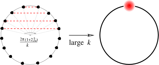
Figure 5: Large k limit of a BPS D1-brane configuration. All the D1-branes collapse to a point.

To probe the low energy behavior at large N we can go to the Alekseev-Recknagel-Schomerus limit (ars limit) [44] where we consider the theory at energies $E$ such that:

$$\alpha^{\prime}E^{2}\to 0\ ,\ \ \lambda\ E^{2}=\alpha^{\prime}k\ E^{2}\to\infty\ ,\ \ \hat{\jmath}_{a}\ \text{fixed}.$$ (59)

In this limit all the D1-branes collapse to a point on the boundary of the disc (fig. 5). From the LST point of view we are in the regime of strong ’t Hooft coupling. Thus we expect to get in this limit some matrix quantum mechanics containing degrees of freedom of strongly coupled Little String Theory at large $k$. We have chosen the limit such that all the states with masses below the inverse of the string length contribute.

We want now to compute the effective action in the ARS limit. All the massive states that we described at the beginning of these section (those with small mass compared to the inverse of the string length) will then contribute because their mass goes to zero. The non-trivial interactions come from the boundary three-point function. Since the $SL(2,\mathbb{R})/U(1)\$part of the CFT is always in the trivial representation it presumably won’t give non-trivial contribution. On the other hand the $SU(2)$ part is non-trivial but reduces in this limit to the matrix multiplication [44] of a fuzzy gauge theory. However this beautiful construction does not directly apply to our case. Indeed according to our analysis of the spectrum of light states on the D1-branes, for any $j$ only states with $n=0$ of the representation survives the low energy limit. Therefore there is no standard enhancement of (fuzzy) gauge symmetry on the W-bosons of LST.

However in the present case we still have a ring of massless states labeled by the spin $j$ of the $SU(2)$ representations coming from the various massive multiplets discussed above. Their fusion rule is given by:

$$V_{j}(x_{1})V_{j^{\prime}}(x_{2})=\sum_{j^{\prime\prime}}\left[\begin{array}[]{ccc}j&j^{\prime}&j^{\prime\prime}\\ 0&0&0\end{array}\right]\left\{\begin{array}[]{ccc}j&j^{\prime}&j^{\prime\prime}\\ \hat{\jmath}&\hat{\jmath}&\hat{\jmath}\end{array}\right\}V_{j^{\prime\prime}}(x_{2})$$ (60)

in terms of the Clebsch-Gordan coefficients $[\cdots]$ and the 6$j$-symbols $\{\cdots\}$. Using this data it should be possible to write the matrix quantum mechanics corresponding to the effective action, much as in [44]. As we argued it may contain the non-trivial dynamics of higgsed $\mathcal{N}=(1,1)$ Little String Theory at large N.

4.3 D4-branes and the beta function of D=4 SYM

Now that we have the exact description of D-branes between NS5-branes, we can ask whether we can recuperate familiar properties from these exact descriptions. Let’s consider the following gauge theory physics [17]. If we consider D4-branes stretching between NS5-branes in type IIA string theory, then the D4-branes pull the NS5-branes and cause a logarithmic bending of the NS5-branes. Since the gauge coupling for the four-dimensional gauge theory on the D4-branes is inversely proportional to the distance between the NS5-branes, we thus recuperate the logarithmic running of the four-dimensional gauge coupling.

Here, we wish to show how the boundary one-point function of the D4-branes stretched between the NS5-branes encodes the beta-function of the gauge theory living on the D4-branes. To realize this, we need to add one step to the above reasoning: the one-point function of the D4-branes encodes the logarithmic bending of the NS5-branes. It is this extra step that we want to demonstrate in this subsection. Let’s consider then our familiar background of NS5-branes, in the near-horizon limit, and the D4-branes stretched between them following [17].

Schematically, the branes fill out the following directions:

$$\begin{array}[]{c|cccccccccc}&0&1&2&3&4&5&6&7&8&9\\ \hline\cr NS5&/\hskip-2.84526pt/&/\hskip-2.84526pt/&/\hskip-2.84526pt/&/\hskip-2.84526pt/&/\hskip-2.84526pt/&/\hskip-2.84526pt/&\perp&\perp&\perp&\perp\\ D4&/\hskip-2.84526pt/&/\hskip-2.84526pt/&/\hskip-2.84526pt/&/\hskip-2.84526pt/&\perp&\perp&/\hskip-2.84526pt/&\perp&\perp&\perp\\ \end{array}\\$$

As we recalled above, the presence of the D4-branes will bend the NS5-branes on which they are attached. More precisely we expect that their position in the $(x^{6},x^{7})$ plane will become a function of the coordinates $(x^{4},x^{5})$. To measure the bending, we will use a holographic reasoning. We know that the position of the fivebranes is encoded in the expectation value of the scalars $X^{6,7,8,9}$, which live on the NS5-brane worldvolume (at low energy, in type IIB). Traceless symmetric combinations of the scalars are holographically dual to particular BPS closed string vertex operators. Using the holographic dictionary of [8][45] we can thus translate the computation of an expectation value of the transverse scalars on the NS5-brane worldvolume (i.e. the computation of the profile of the NS5-branes) into a computation in the bulk worldsheet conformal field theory. However this dictionary is known only in type IIB (i.e. for $\mathcal{N}=(1,1)$ little string theory) thus we have to start from this T-dual type IIB setup. The relevant operators are:

$$\tilde{\text{Tr}}(B^{2j+2})\sim V_{j}(p^{\mu})=e^{-\varphi-\tilde{\varphi}}\Phi^{SU(2)/U(1)\ (2,2)}_{j,j+1,j+1}\ \Phi^{SL(2)/U(1)\ (0,0)}_{\tilde{\jmath},j+1,j+1}\ e^{ip_{\mu}X^{\mu}}$$ (61)

in terms of the complexified scalar $B=X^{6}+iX^{7}$. The value of $\tilde{\jmath}$ is fixed by the on-shell condition of the string theory. From the holographic point of view, these non-normalizable vertex operators correspond to off-shell operators in the dual little string theory, see [45] for details. To find the (change of the) expectation values of these observables of little string theory, we compute the coupling of the boundary states for the D4-branes to the localized states corresponding to (61) in the bulk theory. Thus, we calculate the following quantity:

$$\delta\langle\tilde{\text{Tr}}(B^{2j+2})\rangle(p^{4},p^{5})\sim\langle V_{j}(p^{\mu})|D|\hat{\jmath},\hat{n},\hat{s}_{i},p^{4},p^{5}\rangle\,,$$ (62)

where $D$ is the closed strings propagator in the NS sector:

$$D=\int_{|z|\leqslant 1}\frac{dzd\bar{z}}{z\bar{z}}z^{L_{0}-1/2}\bar{z}^{\bar{L}_{0}-1/2}.$$ (63)

This corresponds to the one point function for the closed string state $|V_{j}(p^{\mu})\rangle$ in the presence of the boundary state $|B_{\hat{\jmath},\hat{n},\hat{s}_{i}}\rangle$. In the following, we will pull the closed string vertex to infinity, i.e. concentrate on the long distance effect of the boundary state, which signals the presence of a closed string tadpole. We will use the change of variables $z=e^{-\pi t+i\theta}$, and using the formula for the one-point function, eq (52), we find the expression:

$$\delta\langle\tilde{\text{Tr}}(B^{2j+2})\rangle(p^{4},p^{5})\sim\pi\int_{0}^{\infty}dt\quad e^{-2\pi t\frac{j(j+1)-(j+1)^{2}}{k}}\langle\Phi^{SU(2)/U(1)\ (2,2)}_{j,j+1,j+1}\Phi^{SL(2)/U(1)\ (0,0)}_{\tilde{\jmath},j+1,j+1}|\hat{\jmath},\hat{n},\hat{s}\rangle$$

$$e^{-\pi tp_{\mu}p^{\mu}}\langle p_{4},p_{5}|\hat{x}^{4},\hat{x}^{5}\rangle_{D}\ \langle p_{0},\cdots,p_{3}|0\rangle\hskip-1.42262pt\rangle_{N}$$

$$=\pi\int_{0}^{\infty}dt\quad e^{-2\pi t\frac{j(j+1)-\tilde{\jmath}(\tilde{\jmath}-1)}{k}+\frac{1}{2}(p_{4}^{2}+p_{5}^{2})}\hskip 142.26378pt$$

$$(-)^{\hat{s}}\,\frac{\nu_{k}^{\frac{1}{2}-\tilde{\jmath}}\phantom{\!\!\!\!\!}}{k}\ e^{i(p_{4}\hat{x}^{4}+p_{5}\hat{x}^{5})}e^{-2i\pi\frac{(j+1)\hat{n}}{k}}\ \frac{\sin\pi\frac{(1+2j)(1+2\hat{\jmath})}{k}}{\sqrt{\sin\pi\frac{1+2j}{k}}}\ \frac{\Gamma\left(\tilde{\jmath}+j+1\right)\Gamma\left(\tilde{\jmath}-(j+1)\right)}{\Gamma(2\tilde{\jmath}-1)\Gamma(1+\frac{2\tilde{\jmath}-1}{k})}$$

In the case $\tilde{\jmath}=j+1$, we have a pole of this expression (of the LSZ type in the classification of [45]) corresponding to a massless localized mode, and we take the residue to find the coupling. Then we can integrate over $t$ and Fourier transform on $p_{4}$ and $p_{5}$. To compute the expectation value, we take the residue at the discrete pole in the second gamma function in the numerator. It leads to the expression:

$$\langle\tilde{\text{Tr}}(B^{2j+2})\rangle(x^{4},x^{5})=-\frac{\log v}{2\pi}(-)^{\hat{s}}\,\frac{\nu_{k}^{-\frac{1}{2}-j}\phantom{\!\!\!\!\!}}{k}\ e^{-2i\pi\frac{(j+1)\hat{n}}{k}}\ \frac{\sin\pi\frac{(1+2j)(1+2\hat{\jmath})}{k}}{\sqrt{\sin\pi\frac{1+2j}{k}}}\ \frac{\Gamma\left(2j+2\right)}{\Gamma(2j+1)\Gamma(1+\frac{2j+1}{k})}\,,$$

$$\text{with}\ v^{2}=(x_{4}-\hat{x}_{4})^{2}+(x_{5}-\hat{x}_{5})^{2}.$$

(65)

fffffffffffffffffffffffff

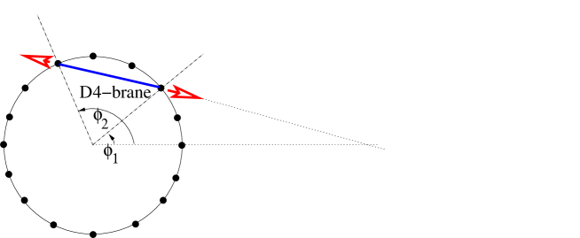
Figure 6: Deformation of the ring of NS5-branes by a D4-brane.

Let us now interpret this result geometrically. We started out with a configuration of five-branes on a circle, corresponding to the following expectation value for the complex scalar field $B$:

$$\langle B\rangle=\rho_{0}\ \text{diag}(1,e^{2i\pi/k},\cdots,e^{2i\pi(k-1)/k}),$$ (66)

before we put any D4-branes into the system. Then we stretched a D4-brane of parameters $\hat{\jmath},\hat{n}$ between two NS5-branes of the ring, located at $\phi_{1}=\frac{\pi(\hat{n}-2\hat{\jmath}-1)}{k}$ and $\phi_{2}=\frac{\pi(\hat{n}+2\hat{\jmath}+1)}{k}$ (see fig. 6). Then, following the geometrical picture, we expect that the expectation value of the operator $B$ will be modified as follows:

$$\langle B\rangle\sim\text{diag}\left(1,\cdots,e^{i\pi(\hat{n}-2\hat{\jmath}-1)/k}-i\lambda e^{i\pi\hat{n}/k}\log v,\cdots,e^{i\pi(\hat{n}+2\hat{\jmath}+1)/k}+i\lambda e^{i\pi\hat{n}/k}\log v,\cdots\right)\,,$$ (67)

where $\lambda$ is an expansion parameter. The variation in the trace of $B^{2j+2}$ is:

$$\delta\langle\text{Tr}(B^{2j+2})\rangle\sim 2i\lambda(2j+2)e^{2i\pi\frac{\hat{n}(j+1)}{k}}\sin\frac{\pi}{k}(2j+1)(2\hat{\jmath}+1)\log v.$$ (68)

This has to be compared with the holographic computation, eq. (65). In particular, the functional dependence in the geometrical parameters $(\hat{\jmath},\hat{n})$ matches precisely. This convincingly demonstrates that the one-point function on the D4-branes allows for the computation of the logarithmic bending of the NS5-branes, which was the extra step we wished to demonstrate. As a side remark, note that we can also check that there is no tadpole for the scalar $A=X^{8}+iX^{9}$. In fact using the dictionary, they correspond to the operators:

$$\tilde{\text{Tr}}(A^{2j+2})\sim V_{j}(p^{\mu})=e^{-\varphi-\tilde{\varphi}}\Phi^{SU(2)/U(1)\ (2,2)}_{j,j+1,-(j+1)}\ \Phi^{SL(2)/U(1)\ (0,0)}_{\tilde{\jmath},j+1,-(j+1)}\ e^{ip_{\mu}X^{\mu}}$$ (69)

which do not couple to the boundary state defined by the one-point function (52). This is expected since the NS5-branes are not pulled in the $x^{8},x^{9}$ directions by the D4-branes.

Note that an alternative interpretation of the computation would be as follows. In [46] the change of the background fields around flat space by a D-brane was computed with roughly the same methods. In fact, the computation can be interpreted as providing the massless closed string tadpoles in the string effective action, which can then be used to determine a new on-shell closed string background. (Reasoning in this way does not require the holographic dictionary.) Both types of reasoning lead to the same conclusion.

In the configuration described here, there is an infrared divergence because the bending of the NS5-branes has a logarithmic profile. As in [17] we could avoid this problem by considering a ”balanced” configuration, i.e. such that the same number of D4-brane end on each side of any NS5-brane. Then the bending of the NS5-branes falls of asymptotically (i.e. for large $v$). However in our case – because the NS5-branes are distributed on a circle and not on a line – it is not possible to obtain such a supersymmetric configuration with only the suspended D4-branes discussed here. We would need to attach to the other side of the NS5-branes semi-infinite D4-branes that will be discussed below.

Further remarks on the beta-function

For completeness, we briefly recall from [17] the precise relation with the computation of the beta-function. For $n$ coincident D4-branes suspended between NS5-branes, we obtain a four-dimensional gauge theory with $\mathcal{N}=2$ supersymmetry. It contains an $SU(n)$ gauge multiplet and no hypermultiplets. It is also possible to add fundamental matter to the gauge theory by adding D6-branes to the setup – which are obtained from the D3-branes discussed below by T-duality along $x^{1,2,3}$.

Calling $\ell(v)$ the distance between a point on the NS5-branes and the point where the D4-branes are attached, the running of the coupling constant is given by:

$$\frac{1}{g_{\textsc{ym}}^{2}(v)}=\frac{\ell(v)}{g_{string}}.$$ (70)

To fix the precise relative coefficient we first complexify the gauge coupling:

$$\tau = \frac{\theta}{2\pi}+\frac{4\pi i}{g^{2}}.$$ (71)

We then observe that the monodromy that the gauge coupling picks up as we change branch in the log-function should correspond to a trivial operation in the gauge theory. The elementary monodromy naturally corresponds to the smallest trivial shift of the theta-angle: $\theta\rightarrow+2\pi$. So, for one D4-brane, we put:

$$-i\tau(v) = -2\log(v).$$ (72)

(To fix the smallest multiple possible, we have made use of the fact that we can add other D4-branes to this picture that will contribute flavors to the ${\cal N}=2$ low-energy gauge theory [17]. That leads to the prefactor of 2 in the above formula.) The sign of the beta-function is determined by considering the direction of the bending of the NS5-branes due to the attached D4-branes. When we generalize this picture to $N$ D4-branes, we obtain:

$$-i\tau(v) = -2N\log(v).$$ (73)

which coincides with the beta-function of $SU(N)$ $N=2$ SYM. The above can be interpreted as a way of fixing the overall coefficients in our computation. It should be clear that if we perform our computation very carefully, we would be able to obtain the precise prefactor, and the beta-function of $N=2$ SYM. (See e.g.[46] for the relevant techniques and a flat space example.) It would be interesting to nail down the overall coefficient, but we haven’t attempted to do so.

In this context, we would moreover like to recall yet another way to compute the beta-function of $N=2$ SYM, using a different holographic set-up in which fractional branes carry the gauge theory that is holographically dual to their corresponding supergravity solution. The supergravity solution is then shown to encode the beta-function [47].

Finally, we would like to mention the intriguing possibility of determining the $N=1$ SYM beta-function from the backreaction of a D3-brane (which can be thought of as the tensor product BCFT of a D3-brane in four-dimensional flat space and the D0-brane of the cigar) in non-critical six-dimensional string theory (see e.g.[48][29][49]). It will be interesting to apply the technique we used here for determining the beta-function in this less supersymmetric setting. The general idea is that the one-point function of the brane encodes sufficient information to determine the running of the coupling that lives on the brane (by open-closed string duality).

4.4 Boundary states for the cylindrical D3-branes

In this section we construct exact descriptions of the first class of D3-branes orthogonal to the NS5-branes in type IIB string theory, of which we discussed the semi-classical description in section 3. We concentrate on the D3-branes which we constructed in the T_ψ-dual picture described by the orbifold of the product of cosets, see eq. (LABEL:firstd3profile). In this T-dual type IIA string theory, we combine the two D1-branes in the respective cosets, and look for the regular brane in the orbifold, i.e. we construct the brane by summing a particular brane and all its images under the orbifold operation. It corresponds to the regular representation of the orbifold group.

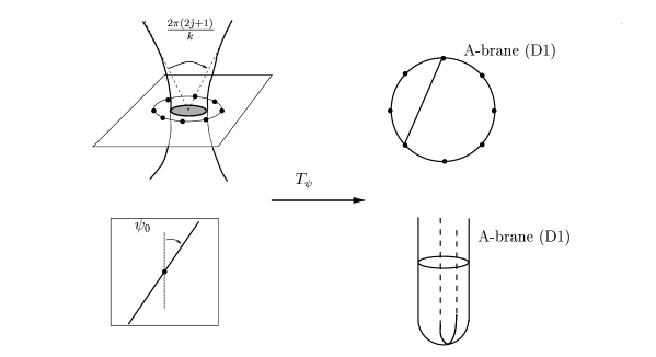
Figure 7: Geometry of the D3-branes and its T-dual, in the case $r_{0}=0$. For large $r$ the D3-brane asymptotes a cone, corresponding to a symmetric D2-brane of $SU(2)$ and a Neumann D-brane (FZZ) of the linear dilaton direction. The intersection of the D3-brane with the plane $x^{8}=x^{9}=0$ is a disc, i.e. a D2-brane of the coset $SU(2)/U(1)$.

The semi-classical picture of the brane in the NS5-brane background is:

$$\begin{array}[]{c|cccccccccc}&0&1&2&3&4&5&6&7&8&9\\ \hline\cr NS5&/\hskip-2.84526pt/&/\hskip-2.84526pt/&/\hskip-2.84526pt/&/\hskip-2.84526pt/&/\hskip-2.84526pt/&/\hskip-2.84526pt/&\perp&\perp&\perp&\perp\\ D3&/\hskip-2.84526pt/&\perp&\perp&\perp&\perp&\perp&/\hskip-2.84526pt/&/\hskip-2.84526pt/&/\hskip-2.84526pt/&\perp\\ \end{array}\\$$

We combine the profiles of the coset D-branes as indicated in the semi-classical analysis (see fig 7). What we obtain from eq. (LABEL:firstd3profile) is a non-trivial D3-brane with, for $r_{0}=0$, a ”cylinder” section near the plane $x^{8}=x^{9}=0$ going through the ring of five-branes, and connecting smoothly with a cone of opening angle $2\pi(2\hat{\jmath}+1)/k$ on both sides. For $r_{0}\neq 0$, the geometry is more involved and in particular the D3-brane avoids the plane $x^{8}=x^{9}=0$.

To construct this D3-brane, we have first to consider a D1-brane in the cigar with the profile (with parameters $\psi_{0}$ and $r_{0}$):

$$\sinh r\sin(\chi-\psi_{0}) = \sinh r_{0}$$ (74)

and then a D1-brane in the T-bell with geometry (with parameters $\phi_{0}$ and $\theta_{0}$):

$$\cos\theta\sin(\chi-\phi+\phi_{0}) = \cos\theta_{0}.$$ (75)

Their exact one-point functions (or Cardy states) are described in terms of the one-point functions. For the $SU(2)/U(1)$ part, we have (e.g. in the NS sector)

$$\langle V^{j^{\prime}}_{n^{\prime}}\rangle_{\hat{\jmath}\hat{n}} = \frac{1}{k}\frac{\sin\left(\frac{\pi(2\hat{\jmath}+1)(2j^{\prime}+1)}{k}\right)}{\sqrt{\sin(\frac{\pi(2j^{\prime}+1)}{k})}}e^{\pi i\hat{n}n^{\prime}/k}$$ (76)

with $\theta_{0}$ and $\phi_{0}$ given by (51). For the $SL(2,\mathbb{R})/U(1)\$part, the one-point function reads:

$$\langle\Phi^{j}_{nw}\rangle_{r_{0},\psi_{0}} = \delta_{w,0}\nu^{1/2-j}\frac{1}{\sqrt{2}}e^{in\psi_{0}}$$ (77)

$$\left[e^{-r_{0}(-2j+1)}+(-1)^{n}e^{r_{0}(-2j+1)}\right]\frac{\Gamma(1-2j)\Gamma(1+\frac{1-2j}{k})}{\Gamma(1-j+\frac{n}{2})\Gamma(1-j-\frac{n}{2})}$$

where the chiral momenta are $m=(n+kw)/2$ and $\bar{m}=-(n-kw)/2$.

We can now sum over $\mathbb{Z}_{k}$ copies of these branes to obtain boundary states of regular branes described by the product of one-point functions of the cosets. The one-point functions for the sum over copies of branes is the sum of the one-point functions for the individual copies. We thus sum over $l\in\mathbb{Z}_{k}$ the boundary states labeled by $(\psi_{0}+2\pi l/k,\hat{n}+2l)$. We obtain the one-point functions:

$$\langle\Phi^{j}_{nw}V^{j^{\prime}}_{-n-k\tilde{w}}\rangle_{r_{0}\psi_{0},\hat{\jmath\,}\hat{n}}=\delta_{w,0}\nu^{1/2-j}\frac{1}{\sqrt{2}}\left[e^{-r_{0}(1-2j)}+(-1)^{n}e^{r_{0}(1-2j)}\right]$$

$$\frac{\Gamma(1-2j)\Gamma(1+\frac{1-2j}{k})}{\Gamma(1-j+\frac{n}{2})\Gamma(1-j-\frac{n}{2})}\frac{\sin(\frac{\pi(2\hat{\jmath}+1)(2j^{\prime}+1)}{k+2})}{\sqrt{\sin(\frac{\pi(2j^{\prime}+1)}{k})}}e^{in\psi_{0}}$$

$$e^{-\pi i\frac{\hat{n}n}{k}}e^{-\pi i\tilde{w}\hat{n}},$$ (78)

and we can absorb the second to last phase factor into a redefinition of the label $\psi_{0}$. Note that $\tilde{w}$ keeps track of whether the $U(1)$ quantum numbers of the two cosets sum up to an even or and odd multiple of $k$. In the GSO-projected closed string spectrum (47), there is an additional $\mathbb{Z}_{2}$ orbifolding such that the charges of the cosets are identified modulo $2k$. In the lightcone gauge, the boundary conditions along the flat directions corresponding to worldvolume of the five-brane of type A (label $\hat{s}_{1}$) for the coordinates $(x^{2},x^{3})$ and B (label $\hat{s}_{2}$) for $(x^{4},x^{5})$. Then putting everything together, and using the labeling of the quantum number of the closed string partition function (47), we find that the one-point function for the D3-brane in the NS5-brane background is given by:

$$\langle\ V_{j^{\prime}m\bar{m}\,jw_{L}w_{R},{\bf p}}^{(s_{i})\ (\bar{s}_{i})}\ \rangle^{D3}_{\hat{\jmath},r_{0},\psi_{0},\hat{s}_{i},{\bf\hat{y}}}=\frac{\nu_{k}^{\frac{1}{2}-j}}{2}\ \delta_{m,-\bar{m}}\delta_{m+2kw_{L},-\bar{m}+2kw_{R}}\ \delta_{s_{1},\bar{s_{1}}}\delta_{s_{2},-\bar{s_{2}}}\delta_{s_{3},-\bar{s_{3}}}\delta_{s_{4},\bar{s_{4}}}\,\delta(p^{5})$$

$$e^{i\sum_{i=0}^{4}p^{i}\hat{y}^{i}}e^{i\frac{\pi}{2}\sum_{i}s_{i}\hat{s}_{i}}\ e^{-i\psi_{0}(m+kw)}\frac{\sin\pi\frac{(1+2j^{\prime})(1+2\hat{\jmath})}{k}}{\sqrt{\sin\pi\frac{1+2j^{\prime}}{k}}}$$

$$\left\{e^{-r_{0}(1-2j)}+(-)^{m-s_{4}}e^{r_{0}(1-2j)}\right\}\frac{\Gamma(1-2j)\Gamma(1+\frac{1-2j}{k})}{\Gamma(1-j-\frac{m-s_{4}}{2}-kw)\Gamma(1-j+\frac{m-s_{4}}{2}+kw)}.$$

Note that this one-point function contains only poles of the “bulk” type associated to infinite volume divergences, and consequently the D3-branes do not couple to the discrete representations of $SL(2,\mathbb{R})/U(1)\$.

Open string partition function

We wish to to compute the open string partition function coming from these boundary states. The overlap between two of those boundary states give the following annulus amplitude in the closed string channel:

$$Z_{closed}^{D3}(\tilde{\tau})=\frac{1}{\sqrt{2k}}\ \int d^{5}p\ \frac{\tilde{q}^{\frac{1}{2}{\bf p}^{2}}}{\eta(\tilde{\tau})^{4}}\ e^{i{\bf p\cdot(\hat{y}-\hat{y}^{\prime})}}$$

$$\frac{1}{2}\sum_{a,b=0}^{1}\sum_{\{\nu_{i}\}\in(\mathbb{Z}_{2})^{4}}(-)^{a}(-)^{b(1+\sum_{i}\nu_{i})}e^{i\frac{\pi}{2}\sum(a+2\nu_{i})(\hat{s}_{i}^{\prime}-\hat{s}_{i})}\chi^{(a+2\nu_{1})}\chi^{(a+2\nu_{2})}$$

$$\sum_{2j^{\prime}=0}^{k-2}\sum_{m\in\mathbb{Z}_{2k}}\frac{S_{\hat{\jmath}}^{\ j^{\prime}}S_{\hat{\jmath\,}^{\prime}}^{\ j^{\prime}}}{S_{0}^{\ j^{\prime}}}\mathcal{C}_{m}^{j\ (a+2\nu_{3})}(\tilde{\tau})$$

$$\int_{0}^{\infty}dP\sum_{w\in\mathbb{Z}}\frac{\cosh 2\pi P+(-)^{m-a}}{\sinh 2\pi P\sinh 2\pi P/k}e^{i(\varphi_{0}^{\prime}-\varphi_{0})(m+2kw)}$$

$$\left[\cos 2P(r_{0}-r_{0}^{\prime})+(-)^{m-a}\cos 2P(r_{0}+r_{0}^{\prime})\right]ch_{c}^{(a+2\nu_{4})}(P,\frac{m}{2}+kw,\tilde{\tau}).$$ (80)

To obtain a well-defined expression in the open string channel, we consider the relative partition function with respect to a reference one with parameters $(r_{\ast},r_{\ast}^{\prime})$, and, to (possibly) preserve supersymmetry, we choose the parameters $(\psi_{0},\psi_{0}^{\prime})$ of the reference branes to be equal to those of the original branes. After a modular transformation we get the following annulus amplitude in the open string channel:

$$Z_{open}=\sqrt{-i\tau}\ \frac{q^{\frac{1}{2}\left(\frac{\bf\hat{y}-\hat{y}^{\prime}}{2\pi}\right)^{2}}}{\eta(\tau)^{4}}$$

$$\sum_{\{\upsilon_{i}\}\in(\mathbb{Z}_{2})^{4}}\frac{1}{2}\sum_{a,b=0}^{1}(-)^{b}(-)^{a(1+\sum_{i}\upsilon_{i})}\chi^{(b+2\upsilon_{1}+\hat{s}_{1}^{\prime}-\hat{s}_{1})}\chi^{(b+2\upsilon_{2}+\hat{s}_{2}^{\prime}-\hat{s}_{2}))}\int_{0}^{\infty}dP\ \sum_{j=0}^{k-2}\sum_{n\in\mathbb{Z}_{2k}}N^{j}_{\hat{\jmath}\ \hat{\jmath\,}^{\prime}}\sum_{W\in\mathbb{Z}}$$

$$\mathcal{C}^{j\ (b+2\upsilon_{3}+\hat{s}_{3}^{\prime}-\hat{s}_{3})}_{n}\left\{\frac{\partial\log\frac{R(P|r_{0},r_{0}^{\prime})}{R(P|r_{\ast},r_{\ast}^{\prime})}}{2i\pi\partial P}\,ch_{c}^{(b+2\upsilon_{4}+\hat{s}_{4}^{\prime}-\hat{s}_{4})}\left(P,\frac{n}{2}+kW-\frac{k(\psi_{0}^{\prime}-\psi_{0})}{2\pi}\right)\right.\qquad\qquad$$

$$+\left.\frac{\partial\log\frac{R(P|r_{0},-r_{0}^{\prime})}{R(P|r_{\ast},-r_{\ast}^{\prime})}}{2i\pi\partial P}\,ch_{c}^{(b+2\upsilon_{4}+\hat{s}_{4}^{\prime}-\hat{s}_{4}+2)}\left(P,\frac{n}{2}+k(W+\nicefrac{{1}}{{2}})-\frac{k(\psi_{0}^{\prime}-\psi_{0})}{2\pi}\right)\right\}$$

(81)

using the modular transformations of the continuous characters, and the reflection amplitude computed in [50], both given in appendix A. Thus we have constructed the exact one-point function of the D-brane whose profile in the T-dual NS5-brane picture we have discussed before. We thought it useful to present the Cardy check for the regular brane to illustrate the relevant techniques in detail, although it is known to be satisfied by construction (i.e. by the fact that it is a sum over branes for which the Cardy computation has been performed).

This channel duality also gives explicitly the open string partition function. We observe that, to get a supersymmetric spectrum of open strings stretched between the two D-branes, one has to impose the condition:

$$\frac{\psi_{0}^{\prime}-\psi_{0}}{\pi}+\sum_{i}(\hat{s}_{i}^{\prime}-\hat{s}_{i})=0\mod 4$$ (82)

such that the angular positions of the D3 branes at infinity in the cigar directions and their orientations coincide. Note also that the parameter $r_{0}$, describing the distance of nearest approach of the D3-branes to the plane of NS5-branes has no role in the supersymmetry of the open string spectrum. Indeed D3-branes with different parameters are separated but parallel in the flat coordinates discussed in detail in section 3.

The supersymmetric open string spectrum contains both states with integer windings (first term) and half-integer windings (second term). The latter correspond to open strings stretched between the two halves of the D1-brane of the cigar. By going back to the conformally flat Cartesian coordinates (10) we observe that these open strings are of arbitrary length. Indeed the cigar is ”unfolded” to the plane $(x^{8},x^{9})$. Because of the curved background generated by the NS5-branes, they are of finite mass.

4.5 Boundary states for the second class of D3-branes

In section 3, we discussed the geometry of a second D3-brane, see (44). We will provide its exact description in this section. It is constructed by tensoring D1-branes in the trumpet with D1-branes of the bell. We will need first to discuss the former.

The D1-branes in the trumpet

The D1-branes of the trumpet – the vector coset $SL(2,\mathbb{R})/U(1)$ – are T-dual to D2-branes of the cigar (the axial coset). The ”cut” D2-branes of the supersymmetric cigar (i.e. with $c<1$, see eq. (27)) were constructed in [35], following the results of [28] for the bosonic case. These D2-branes carry a magnetic charge localized near the tip of the cigar, inducing a D0-brane charge. They descend from the $H_{2}$ brane in Euclidean AdS₃ which is consistent with a factorization constraint [51]. However the open string annulus amplitude for these D2-branes in the cigar [35] contains a D0-like contribution – induced by the magnetic flux – with negative multiplicities, so they are not consistent with the Cardy condition. Therefore for generic $k$ only the D2-brane without magnetic field is consistent. However, as we show in appendix D, when $k$ is integer – and this is the case in the present setup – all the unwanted features disappear, and one obtains perfectly consistent boundary states, containing only couplings to the continuous representations.

Let us now translate the result from the cigar CFT (the axial coset) to the trumpet CFT (the vector coset). The vector coset is characterized by left and right momenta $(\nicefrac{{\tilde{n}-k\tilde{w}}}{{2}},\nicefrac{{\tilde{n}+k\tilde{w}}}{{2}})$, which are related to the $SL(2,\mathbb{R})$ quantum numbers as $m+\bar{m}=\tilde{n}$ and $m-\bar{m}=-k\tilde{w}$. This theory can be obtained, for $k$ integer, by a $\mathbb{Z}_{k}$ orbifold of the cigar, followed by a T-duality as has been shown in [53]. In this case $\tilde{n}/k$ is identified with the fractional winding of the orbifold of the cigar and $k\tilde{w}$ with the momentum modes allowed by the $\mathbb{Z}_{k}$ projection. From these D2-branes covering the cigar we will obtain by T-duality D1-branes of the trumpet of equation:

$$\cosh r\sin(\psi-\psi_{0})=\sin\sigma$$ (83)

thus reaching the singularity $r=0$. By this construction it is clear that the zero-mode $\psi_{0}$ is quantized as $\psi_{0}=\sigma+\nicefrac{{2\pi\hat{p}}}{{k}}$. From the semi-classical point of view, it is related to the issue vortex singularities for the D2-branes reaching the tip of the cigar discussed in sect. 3.1. Thus starting from the one-point function for the ”cut” D2-brane in the cigar given in appendix D, we obtain the following one-point function for the D1-branes of the trumpet reaching the singularity:

$$\langle\Phi^{j,(s)}_{\tilde{n}\,\tilde{w}}\rangle_{\hat{s},\hat{n}}=\frac{\nu_{k}^{1/2-j}}{4\pi k\sqrt{2}}\ \delta_{\tilde{w},0}\ \delta_{s,\hat{s}}\ e^{-i\pi\frac{s\hat{s}}{2}}e^{\frac{i\pi\hat{n}\tilde{n}}{k}}$$

$$\Gamma\left(2-2j\right)\Gamma\left(\frac{1-2j}{k}\right)\frac{\Gamma\left(j+\frac{\tilde{n}-s}{2}\right)}{\Gamma\left(1-j+\frac{\tilde{n}-s}{2}\right)}\left[e^{i\sigma(1-2j)}+(-)^{\tilde{n}-s}e^{-i\sigma(1-2j)}\right]$$ (84)

This one-point function contains only couplings to the continuous representations. Indeed, we find the following annulus amplitude in the closed string channel:

$$Z^{D2}_{\sigma\sigma^{\prime}}(-1/\tau,\nu/\tau) =\frac{1}{4k}\int dP\sum_{\tilde{n}\in\mathbb{Z}}\sum_{s\in\mathbb{Z}_{4}}\ e^{-i\pi\frac{s(\hat{s}^{\prime}-\hat{s})}{2}}\ e^{\frac{i\pi(\hat{n}^{\prime}-\hat{n})\tilde{n}}{k}}\$$

$$\frac{\cosh 2P(\sigma+\sigma^{\prime})+(-)^{\tilde{n}-s}\cosh 2P(\sigma-\sigma^{\prime})}{\sinh 2\pi P\sin 2\pi P/k}\ \ ch_{c}^{(s)}\left(j,\frac{\tilde{n}}{2};-1/\tau,\nu/\tau\right)$$ (85)

Thus in the open string channel we find the following consistent result:

$$Z^{D1_{T}}_{open}(\tau)=\int_{0}^{\infty}dP^{\prime}\sum_{w}\left[\frac{\partial\log\frac{R(P|i\sigma,i\sigma^{\prime})}{R(P|i\sigma_{\ast},i\sigma_{\ast}^{\prime})}}{2i\pi\partial P}\ ch_{c}^{(\hat{s}^{\prime}-\hat{s})}(P,\hat{n}^{\prime}-\hat{n}+kw;\tau)\right.$$ (86)

$$+\frac{\partial\log\frac{R(P|i\sigma,-i\sigma^{\prime})}{R(P|i\sigma_{\ast},-i\sigma_{\ast}^{\prime})}}{2i\pi\partial P}\ ch_{c}^{(2+\hat{s}^{\prime}-\hat{s})}(P,\hat{n}^{\prime}-\hat{n}+k(w+1/2);\tau)$$ (87)

checking the normalization of the one-point function. Thus we have a family of D1-branes in the vector coset $SL(2,\mathbb{R})$ consistent both with factorization and the modular bootstrap. Note that they give almost the same open string partition function as the D1-branes of the cigar, except that the parameter of the D-brane entering into the reflection amplitudes is imaginary.

At least for parallel D1-branes ($\hat{n}^{\prime}=\hat{n}$), we can identify the terms with integer windings $w$ in eq. (87) as corresponding to open strings with both ends on the same half D1-brane, and the terms with half-integer windings as corresponding to open strings with one end on each half D1-brane. The two bracketed terms in (84) correspond to the two different halves. In opposition to the D1-branes in the cigar, these two pieces should be thought as independent D-branes since their worldvolume are not connected.

The one-point function of the D3-brane

We would like now to construct the boundary state for the second class of D3-branes orthogonal to the NS5-branes discussed in section 3. This D3-brane is obtained from the alternative T-dual geometry (18). It is made of a ”cut” D1-brane of the trumpet and a D1-brane of the bell. After T-duality we obtain the complicated hypersurface given by eq. (44), with $c=\sin\sigma$. The parameter $\sigma$ is quantized as $\sigma\in\pi\mathbb{Z}/k$ as we shall discuss again in the next section. The shape of the D3-brane is depicted in fig. 8 for the simplest case $\sigma=0$ (more precisely we have two disconnected antipodal copies of this D3-brane). This D3-brane connects a finite-size D1-brane inside the ring of fivebranes with a ”conical” D3-brane at infinity, see eq. (44). In particular the intersection with the plane $x^{8}=x^{9}=0$ is made of two straight half-lines.

Figure 8: Geometry of the D3-branes and its T-dual, in the case $\sigma=0$. For large $r$ the D3-brane asymptotes a cone, corresponding to a symmetric D2-brane of $SU(2)$ and a Neumann D-brane (FZZ) of the linear dilaton direction. The intersection of the D3-brane with the plane $x^{8}=x^{9}=0$ is made of a D1-brane of the bell – for the interior of the ring of fivebranes – and two (half) D1-branes of the trumpet – for the exterior of the ring.

We are now ready to write the complete boundary states starting from the boundary state for the D1-brane of the trumpet discussed above. Following the same logic as the previous example, we gather the contributions from the various factors and obtain after the $\mathbb{Z}_{k}$ orbifold the following one-point function for the Hanany-Witten D3-brane:

$$\langle\ V_{j^{\prime}m\bar{m}jw_{L}w_{R},{\bf p}}^{(s_{i})\ (\bar{s}_{i})}\ \rangle_{\hat{\jmath},\psi_{0},\hat{s}_{i},{\bf\hat{y}}}=\frac{\nu_{k}^{\frac{1}{2}-j}}{\pi k\sqrt{2}}\ (-)^{kw}\delta_{m,\bar{m}}\delta_{m+2kw_{L},\bar{m}-2kw_{R}}\ \delta_{s_{1},\bar{s_{1}}}\delta_{s_{2},-\bar{s_{2}}}\delta_{s_{3},\bar{s_{3}}}\delta_{s_{4},-\bar{s_{4}}}\,\delta(p^{5})$$

$$e^{i\sum_{i=0}^{4}p^{i}\hat{y}^{i}}e^{i\frac{\pi}{2}\sum_{i}s_{i}\hat{s}_{i}}\ \frac{\sin\pi\frac{(1+2j^{\prime})(1+2\hat{\jmath})}{k}}{\sqrt{\sin\pi\frac{1+2j^{\prime}}{k}}}\ e^{\frac{i\pi(\hat{n}^{\prime}-\hat{n})\tilde{n}}{k}}$$

$$\Gamma\left(2-2j\right)\Gamma\left(\frac{1-2j}{k}\right)\frac{\Gamma\left(j+\frac{\tilde{n}-s_{4}}{2}+kw\right)}{\Gamma\left(1-j+\frac{\tilde{n}-s_{4}}{2}+kw\right)}\left[e^{i\sigma(1-2j)}+(-)^{\tilde{n}-s_{4}}e^{-i\sigma(1-2j)}\right]$$

This one-point function contains only couplings to the continuous representations of the $SL(2,\mathbb{R})/U(1)$ theory. The computation of the annulus amplitude is quite similar to the previous D3-brane. Indeed as we saw the only difference being the parameters of the reflection amplitude, and the fact that the $U(1)$ label is quantized to $\nicefrac{{2\pi\hat{n}}}{{k}}$. This last point is related to the fact that, while the $SO(2)$ rotational isometry is preserved in the $(x^{8},x^{9})$ plane, it is broken to $\mathbb{Z}_{k}$ in the $(x^{6},x^{7})$ plane by the ring of five-branes.

So, we can skip the details of the computation of the overlap of boundary states, and give the result for the open string partition function:

$$Z_{open}=\sqrt{-i\tau}\ \frac{q^{\frac{1}{2}\left(\frac{\bf\hat{y}-\hat{y}^{\prime}}{2\pi}\right)^{2}}}{\eta(\tau)^{4}}$$

$$\sum_{\{\upsilon_{i}\}\in(\mathbb{Z}_{2})^{4}}\frac{1}{2}\sum_{a,b=0}^{1}(-)^{b}(-)^{a(1+\sum_{i}\upsilon_{i})}\chi^{(b+2\upsilon_{1}+\hat{s}_{1}^{\prime}-\hat{s}_{1})}\chi^{(b+2\upsilon_{2}+\hat{s}_{2}^{\prime}-\hat{s}_{2}))}\int_{0}^{\infty}dP\ \sum_{2j=0}^{k-2}\sum_{n\in\mathbb{Z}_{2k}}N^{j}_{\hat{\jmath}\ \hat{\jmath\,}^{\prime}}\sum_{W\in\mathbb{Z}}$$

$$\mathcal{C}^{j\ (b+2\upsilon_{3}+\hat{s}_{3}^{\prime}-\hat{s}_{3})}_{n}\left\{\,\frac{\partial\log\frac{R(P|i\sigma,i\sigma^{\prime})}{R(P|i\sigma_{\ast},i\sigma_{\ast}^{\prime})}}{2i\pi\partial P}\ ch_{c}^{(b+2\upsilon_{4}+\hat{s}_{4}^{\prime}-\hat{s}_{4})}\left(P,\frac{n}{2}+kW+\hat{n}-\hat{n}^{\prime}\right)\right.$$

$$+\left.\frac{\partial\log\frac{R(P|i\sigma,-i\sigma^{\prime})}{R(P|i\sigma_{\ast},-i\sigma_{\ast}^{\prime})}}{2i\pi\partial P}\ ch_{c}^{(b+2\upsilon_{4}+2+\hat{s}_{4}^{\prime}-\hat{s}_{4})}\left(P,\frac{n}{2}+k(W+\nicefrac{{1}}{{2}})+\hat{n}-\hat{n}^{\prime}\right)\right\}$$

(89)

The supersymmetry conditions here reads

$$\sum_{i}(\hat{s}_{i}^{\prime}-\hat{s}_{i})-\frac{2(\hat{n}^{\prime}-\hat{n})}{k}=0\ \text{mod}\ 4.$$ (90)

Again the sector with half-integer windings correspond to open strings stretched between the two halves of the D-branes, which have disconnected worldvolumes.

The similarity of the result between both types of D3-branes is expected since both branes asymptote to isomorphic D3-branes of $SU(2)\times\mathbb{R}_{Q}$. Indeed in both cases we get a D2-brane of $SU(2)$ times a Neumann brane of the linear dilaton, the only difference being the position of the S²-brane in the three-sphere, so only the reflection amplitudes – which depends on the physics near the NS5-branes – are different. Due to their different positions they cannot appear simultaneously in a supersymmetric configuration. One can check indeed that the spectrum of open strings stretched between two D3-branes of different types is not supersymmetric.

4.6 Boundary states for the D-rays

Now we wish to consider the semi-infinite D1-branes ending on NS5-branes. As we saw in the semi-classical discussion they are associated to D1-branes in the trumpet, reaching the singularity $r=0$. In the present case it means that they reach the ring of five-branes. As for the D2-branes, the $U(1)$ label of the D1-brane is quantized as $\psi_{0}=\sigma+\nicefrac{{2\pi\hat{p}}}{{k}}$. Moreover, as already stated, if we assume also that the parameter $\sigma$ is quantized as $\sigma\in\pi\mathbb{Z}/k$, we find that the D1-branes have to end on the NS5-branes, see fig. 9.

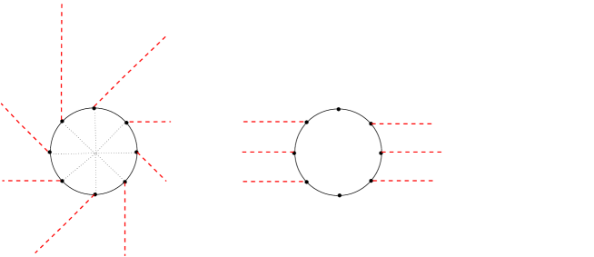
Figure 9: Configurations of D-rays, for fixed $\sigma$ (left) and supersymmetric (right).

The D1-branes ending on the NS5-branes are just the special case $\hat{\jmath}=0$ of the previous D3-branes. So they have the following one-point function:

$$\langle\ V_{j^{\prime}m\bar{m}jw_{L}w_{R},{\bf p}}^{(s_{i})\ (\bar{s}_{i})}\ \rangle_{\hat{\jmath},\psi_{0},\hat{s}_{i},{\bf\hat{y}}}=\frac{\nu_{k}^{\frac{1}{2}-j}}{\pi k\sqrt{2}}\ (-)^{kw}\ \delta_{m,\bar{m}}\delta_{m+2kw_{L},\bar{m}-2kw_{R}}\ \delta_{s_{1},\bar{s_{1}}}\delta_{s_{2},-\bar{s_{2}}}\delta_{s_{3},\bar{s_{3}}}\delta_{s_{4},-\bar{s_{4}}}\,\delta(p^{5})$$

$$e^{i\sum_{i=0}^{4}p^{i}\hat{y}^{i}}e^{i\frac{\pi}{2}\sum_{i}s_{i}\hat{s}_{i}}\ \sqrt{\sin\frac{\pi(1+2j^{\prime})}{k}}\ e^{\frac{i\pi(\hat{n}^{\prime}-\hat{n})\tilde{n}}{k}}$$

$$\Gamma\left(2-2j\right)\Gamma\left(\frac{1-2j}{k}\right)\frac{\Gamma\left(j+\frac{\tilde{n}-s_{4}}{2}+kw\right)}{\Gamma\left(1-j+\frac{\tilde{n}-s_{4}}{2}+kw\right)}\left[e^{i\sigma(1-2j)}+(-)^{\tilde{n}-s_{4}}e^{-i\sigma(1-2j)}\right]$$

and the open string spectrum is the same as (89) by replacing $N^{j}_{\hat{\jmath}\ \hat{\jmath\,}^{\prime}}\to\delta_{j,0}$. Thus it consists only in continuous representations of $SL(2,\mathbb{R})/U(1)\$, with a non-trivial density of states. Asymptotically these D-branes are D0-branes of $SU(2)$ times Neumann D-branes of the linear dilaton. In the semi-classical analysis there was another class of these D1-branes, avoiding the ring of NS5-branes. They are obtained from descent of dS₂ D-branes of Euclidean AdS₃ and a candidate boundary state was found using the modular bootstrap method in [52]. However up to now there is no check of factorization constraints for those D-branes.

4.6.1 The anomalous creation of branes

These D3-branes of the second type are the natural D3-branes to consider the Hanany-Witten effect of anomalous creation of D1-branes. Indeed it is clear from the previous analysis – see fig. 8 and eq. (44) – that such D3-branes of label $\hat{\jmath}$ trap $(2\hat{\jmath}+1)$ NS5-branes inside their worldvolume. It has been argued in [16] from the study of the theory living on the worldvolume of the D3-branes that in such a configuration D1-branes are created whenever the D3-brane crosses a stack of $n$ NS5-branes and traps them. Because the D3-branes are repelled by the NS5-branes a long tube is formed when the D3-branes are pushed far away, and corresponds effectively to a stack of $n$ D1-branes with one end on the NS5-stack and the other end on the D3-brane.

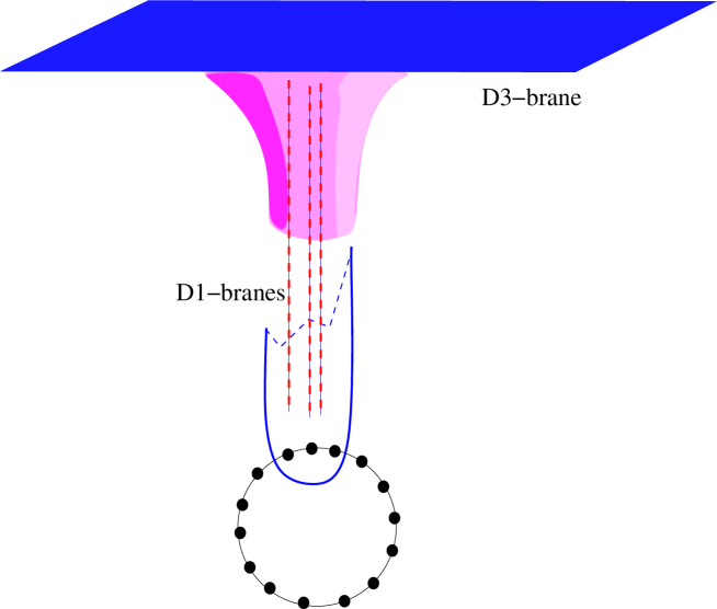
Figure 10: Hanany-Witten configuration with creation of D1-branes.

As was shown in [54], in the supergravity approximation, for coincident NS5-branes it gives simply a cone in the near-horizon limit. In the setup of the ring of NS5-branes that we consider we can have a handle on the worldsheet theory which is weakly coupled, and the distribution of fivebranes is ”resolved”. It allows to show explicitly the link between the label $\hat{\jmath}$ of the D2-brane of $SU(2)$ and the number of NS5-branes trapped by the D3-brane (because we know exactly the shape of the D3-branes around the NS5-branes), and to construct the exact boundary state for this configuration. As it is well known [31, 44] a D2-brane of SU(2) of label $\hat{\jmath}$ can be constructed as a bound state of $(2\hat{\jmath}+1)$ D0-branes. Translated to our setup it means that we can construct our D3-brane trapping $(2\hat{\jmath}+1)$ N55-branes as a bound state of $(2\hat{\jmath}+1)$ D-rays. This fits perfectly with the Hanany-Witten picture. Note that in the near-horizon limit we see only the tip of the tube – made with the D1-branes that have been created – and so it is natural that the D3-brane we consider in the CFT analysis is made only of a bound state of D1-branes. The D3-brane itself lives in the asymptotically flat region that is absent from the double scaling limit considered in this paper, see fig. 10. It would be interesting to find explicitly the supersymmetric solution of the DBI action, in the full asymptotically flat spacetime, corresponding to this D3-brane geometry.

For the first class of D3-branes (the ”cylindrical” D-branes of section 4.4) the story is actually very different. This configuration should be thought – after adding the asymptotic flat region  – as a configuration of two parallel D3-branes widely separated, which are on both sides of the NS5-branes ring. They are connected by a tube of D1-strings going through (for $r_{0}=0$) the ring of fivebranes, see fig. 11.

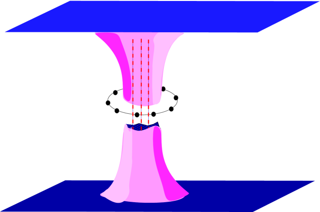
Figure 11: Configuration of two D3-branes linked by a tube of D1-branes going through the ring of fivebranes.

In the double scaling limit considered here we focus on the portion of the tube near the ring of fivebranes. However in this case we can move the D3-brane continuously out of the ring of five-brane in the plane $(x^{8},x^{9})$ by changing the parameter $r_{0}$ of the D3-brane. Indeed as we saw in the section of the D3-brane in this plane is simply a straight line, whose minimal distance to the stack of fivebranes is $\rho_{0}\sinh r_{0}$. At the level of the exact CFT nothing dramatic happens for $r_{0}=0$, i.e. when the tube is indeed lassoed by the fivebranes ring. It corresponds simply to a particular value of the density of states in the open string partition function of eq. (81). It would be interesting to understand such a (Euclidean) wormhole-like configuration from the point of view of the worldvolume gauge theory on the D3-branes.

4.6.2 Hypermultiplets on D3-branes associated to NS5-branes

There is an interesting issue that has been addressed in [16] in the low-energy limit. Configurations of D3-branes ending on NS5-branes were studied (it is simply a T-dual of our setup of D1-branes along the directions $x^{1,2}$) and it was argued that when two stacks of D3-branes ending on two sides of a NS5-brane become ”aligned”, a new massless hypermultiplet appears in the low energy effective action on the D-branes. We would like to study such a phenomenon in our setup, see fig. 12.

aaaaaaaaaaaaaaaaaaaaaaaa

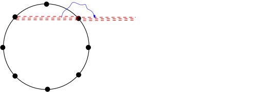
Figure 12: Configuration of two D3-brane stacks ending on both sides of an NS5-brane, with an open string stretched between them.

The stacks of D3-branes are parallel in the $(x^{6},x^{7})$ plane, coincident in the plane $(x^{8},x^{9})$ and at a distance $\delta$ in the directions $x^{3,4,5}$ longitudinal to the NS5-branes. We are interested in computing the spectrum of open strings stretched between a suspended D3-brane of parameters $(\hat{\jmath},\hat{n}=0,\hat{s}=0)$ and a semi-infinite D3-brane of parameters $(\sigma,\hat{n}=0,\hat{s}=0)$. This D-brane setup is supersymmetric. The value of $\sigma$ that we will choose is expected to correspond to aligned D3-branes, thus giving a massless hypermultiplet.

Let us consider for convenience the configuration of D1-branes obtained by T-duality in the directions $x^{1,2}$. The overlap of boundary states for a suspended D1-brane of parameter $\hat{\jmath}$ and a semi-infinite D1-brane of parameter $\sigma$ give, in the closed string channel:

$$Z_{closed}^{\textsc{hyper}}(\tilde{\tau})=\sqrt{\frac{2}{k}}\int d^{5}p\ \frac{\tilde{q}^{\frac{1}{2}{\bf p}^{2}}}{\eta(\tilde{\tau})^{4}}\ e^{i{\bf p\cdot(\hat{y}-\hat{y}^{\prime})}}$$

$$\frac{1}{2}\sum_{a,b=0}^{1}\sum_{\{\nu_{i}\}\in(\mathbb{Z}_{2})^{4}}(-)^{a}(-)^{b(1+\sum_{i}\nu_{i})}\chi^{(a+2\nu_{1})}\chi^{(a+2\nu_{2})}\sum_{2j^{\prime}=0}^{k-2}\sum_{m\in\mathbb{Z}_{2k}}S_{\hat{\jmath}}^{\ j^{\prime}}\mathcal{C}_{m}^{j^{\prime}\ (a+2\nu_{3})}(\tilde{\tau})$$

$$\int dj\ \frac{1}{\sin\pi(j-\frac{m-a}{2})}\sum_{w\in\mathbb{Z}}\left[e^{i\sigma(1-2j)}+(-)^{m-a}e^{-i\sigma(1-2j)}\right]\ ch^{(a+2\nu_{4})}(j,\frac{m}{2}+kw,\tilde{\tau}).$$

(92)

and this expression contains indeed poles for the discrete representations, in contrast to the D2-D2 overlap for integer $k$. The overlap does not contain ”‘bulk” poles at zero radial momentum $j=1/2$ corresponding to infinite volume divergences, which is natural since at the end we will find localized open string states. The integral $\int dj$ contains both and integral over the continuous representations $j=\nicefrac{{1}}{{2}}+iP$ and contributions from the discrete representation whenever there is a pole with non-zero residue. The poles in this expression arises whenever $j-(m-a)/2\in\mathbb{Z}$, i.e. we have a pole for each discrete representation appearing in the closed string spectrum. In the following we will assume that the parameter $\sigma$ is quantized as:

$$\sigma=\frac{\pi(2J-1)}{k}\ ,\ \ 2J\in\mathbb{N}\ ,\ \ \nicefrac{{1}}{{2}}<J<\nicefrac{{k+1}}{{2}}$$ (93)

As we argued earlier for the D1-branes of the trumpet, each of the bracketed terms in eq. (92) correspond to one semi-infinite D1-brane. So let us consider only the first term. Then, using the modular transformation of the extended discrete characters given in appendix A, we find that the contribution from the poles of this expression (together with the continuous couplings) comes from the following discrete spectrum in the open string channel:

$$Z^{\textsc{hyper}}_{\text{open}}=\sqrt{-i\tau}\ \frac{q^{\frac{1}{2}\left(\frac{\delta}{2\pi}\right)^{2}}}{\eta(\tau)^{4}}\sum_{\{\upsilon_{i}\}\in(\mathbb{Z}_{2})^{4}}\frac{1}{2}\sum_{a,b=0}^{1}(-)^{b}(-)^{a(1+\sum_{i}\upsilon_{i})}\chi^{(b+2\upsilon_{1})}\chi^{(b+2\upsilon_{2})}$$

$$\sum_{n\in\mathbb{Z}_{k}+\frac{b}{2}}\mathcal{C}^{\hat{\jmath}\ (b+2\upsilon_{3})}_{2n}(\tau)\ Ch_{d}^{(b+2\upsilon_{4})}(J,n-J;\tau)$$

Let us assume that the D1-branes are coincident in the directions $x^{1,2,3,4,5}$. Then – using a similar analysis as for the suspended D1-branes – this spectrum contains one massless hypermultiplet if $J=\hat{\jmath}+1$, which is perfectly consistent with our geometrical picture. Indeed the massless hypermultiplet corresponds to the open string sectors stretched between the aligned D1-branes of the bell and the trumpet. In the present case we have chosen $\sigma=\nicefrac{{\pi}}{{2}}-\theta_{0}$ and the two D1-branes indeed end on the same NS5-brane according to the geometrical picture given in the previous sections for the various D-branes.

We have then proven that when the D3-branes ending on both sides of the NS5-brane are coincident, a new massless hypermultiplet in the bifundamental appears. This constitutes a worldsheet CFT demonstration of the property understood in [16].

5 Non-BPS D-branes

In this section we comment briefly on the non-BPS D-branes in this background. Some of the relevant boundary states have already be given in [15] but we would like to focus on geometrical aspects, and discuss in some more detail the non-compact branes. As we have seen in the previous sections, the BPS D-branes in the NS5-brane background are, for the non-trivial $SL(2,\mathbb{R})/U(1)\$and $SU(2)/U(1)$ factors, either of A-A type or of B-B type in the T-dual backgrounds. In this case the projection induced by the $\mathbb{Z}_{k}$ orbifold will translate into a spectrum of odd-integral N=2 charges in the open string channel, thus into a space-time supersymmetric spectrum. Apart from the obvious D-branes of wrong dimensionality (i.e. odd-dimensional in type IIA and even-dimensional in type IIB) the non-BPS D-branes are of type A-B or B-A for the CFT of the transverse directions to the five-branes.

5.1 Compact D2-branes

Using the procedure that is by now familiar, we start from D-branes in the T_ψ-dual geometry (17), i.e. the orbifold of the cigar times the T-bell. We can construct a first non-BPS D-brane by starting with a D1-brane of the T-bell and a D0-brane of the cigar CFT (in type IIB). After T-duality, we obtain in type IIA superstrings a non-BPS D2-brane in the NS5-brane background of embedding equations and gauge field:

$$r = 0\ ,\ \ \theta<\theta_{0}$$

$$F = \frac{k}{2\pi}\ \frac{\tan\theta\cos\theta_{0}}{\sqrt{\cos^{2}\theta-\cos^{2}\theta_{0}}}d\theta\wedge d\psi$$ (94)

They correspond to D2-branes of finite size, living in the plane $x^{8}=x^{9}=0$ where the fivebrane sit. Their worldvolume are discs defined by $\theta<\theta_{0}$, contained inside the ring of fivebranes.

Their one-point function is:

$$\langle\ V_{j^{\prime}m\bar{m}jw_{L}w_{R},{\bf p}}^{(s_{i})\ (\bar{s}_{i})}\ \rangle_{\hat{\jmath},\hat{n},\hat{s}_{i},{\bf\hat{y}}}=\sqrt{\frac{2}{k}}\ \nu_{k}^{\frac{1}{2}-j}\ \delta_{m,-\bar{m}}\delta_{m+2kw_{L},\bar{m}-2kw_{R}}\ \delta_{s_{1},\bar{s_{1}}}\delta_{s_{2},-\bar{s_{2}}}\delta_{s_{3},-\bar{s_{3}}}\delta_{s_{4},-\bar{s_{4}}}\,\delta(p^{5})$$

$$e^{i\sum_{i=0}^{4}p^{i}\hat{y}^{i}}e^{i\frac{\pi}{2}\sum_{i}s_{i}\hat{s}_{i}}\ \ \frac{\sin\pi\frac{(1+2j^{\prime})(1+2\hat{\jmath})}{k}}{\sqrt{\sin\pi\frac{1+2j^{\prime}}{k}}}\ \frac{\Gamma\left(j-\frac{s_{4}}{2}+kw\right)\Gamma\left(j+\frac{s_{4}}{2}-kw\right)}{\Gamma(2j-1)\Gamma(1-\frac{1-2j}{k})}.$$

and are normalized with a factor of $\sqrt{2k}$ w.r.t. the BPS suspended D1-branes to satisfy the Cardy condition. Their overlap give the following non-supersymmetric amplitude in the open string channel:

$$Z^{\textsc{w}}_{\text{open}}=\sqrt{-i\tau}\ \frac{q^{\frac{1}{2}\left(\frac{\bf\hat{y}-\hat{y}^{\prime}}{2\pi}\right)^{2}}}{\eta(\tau)^{4}}\sum_{\{\upsilon_{i}\}\in(\mathbb{Z}_{2})^{4}}\frac{1}{2}\sum_{a,b=0}^{1}(-)^{b}(-)^{a(1+\sum_{i}\upsilon_{i})}\chi^{(b+2\upsilon_{1}+\hat{s}_{1}^{\prime}-\hat{s}_{1})}\chi^{(b+2\upsilon_{2}+\hat{s}_{2}^{\prime}-\hat{s}_{2})}$$

$$\sum_{2j=0}^{k-2}\sum_{n\in\mathbb{Z}_{2k}}N^{j}_{\hat{\jmath}\ \hat{\jmath\,}^{\prime}}\ \mathcal{C}^{j\ (b+2\upsilon_{3}+\hat{s}_{3}^{\prime}-\hat{s}_{3})}_{n}(\tau)\ \sum_{r\in\mathbb{Z}_{k}+\frac{b}{2}}Ch_{\mathbb{I}}^{(b+2\upsilon_{4}+\hat{s}_{3}^{\prime}-\hat{s}_{3})}(r;\tau),$$

In this open string spectrum the non-integral part of the N=2 charges of the two coset models are uncorrelated, thus the spectrum is not supersymmetric and contains tachyons (see also [15]). This is related to the instability of the D2-brane of $SU(2)/U(1)$ towards moving to the boundary of the disc.

5.2 Non-BPS non-compact D4-branes

This non-compact D4-brane of type IIA is obtained from the T_ψ-dual background (17), out of a D1-brane of the cigar and a D2-brane of the T-bell. Using the same T-duality techniques as for the BPS D-branes, it gives a non-BPS D4-brane with a non-trivial gauge field:

$$A=\frac{k}{2\pi}\left[\arcsin\left(\frac{\sin\theta_{0}}{\sin\theta}\right)-\theta_{0}\right]\left[d\phi-d\left(\arcsin\frac{\sinh r_{0}}{\sinh r}\right)\right]+\frac{k}{2\pi}\left[\arcsin\left(\frac{\sinh r_{0}}{\sinh r}\right)+\psi_{0}\right]d\psi$$ (96)

whose worldvolume is restricted to the region $r>r_{0}$ and $\theta>\theta_{0}$. For large $r$, all these D4-branes asymptote symmetry-breaking D3-branes of $SU(2)$ (i.e. a B-brane, see [22]) of gauge field

$$A=\frac{k}{2\pi}\left[\arcsin\left(\frac{\sin\theta_{0}}{\sin\theta}\right)-\theta_{0}\right]d\phi$$ (97)

covering the region $\theta>\theta_{0}$, times a Neumann D-brane of the linear dilaton.

The one-point function for these D4-branes is quite similar to the one-point function for cylindrical D3-branes, and is given by:

$$\langle\ V_{j^{\prime}m\bar{m}\,jw_{L}w_{R},{\bf p}}^{(s_{i})\ (\bar{s}_{i})}\ \rangle^{D3}_{\hat{\jmath},\theta_{0},r_{0},\hat{s}_{i},{\bf\hat{y}}}=\sqrt{\frac{k}{2}}\ \nu_{k}^{\frac{1}{2}-j}\ \delta_{m,\bar{m}}\delta_{m+2kw_{L},-\bar{m}+2kw_{R}}\ \delta_{s_{1},\bar{s_{1}}}\delta_{s_{2},-\bar{s_{2}}}\delta_{s_{3},-\bar{s_{3}}}\delta_{s_{4},\bar{s_{4}}}\,\delta(p^{5})$$

$$e^{i\bf{p\cdot y}}e^{i\frac{\pi}{2}\sum_{i}s_{i}\hat{s}_{i}}\ e^{-2ik\psi_{0}w}\frac{\sin\pi\frac{(1+2j^{\prime})(1+2\hat{\jmath})}{k}}{\sqrt{\sin\pi\frac{1+2j^{\prime}}{k}}}\left[e^{-r_{0}(1-2j)}+(-)^{s_{4}}e^{r_{0}(1-2j)}\right]$$

$$\frac{\Gamma(1-2j)\Gamma(1+\frac{1-2j}{k})}{\Gamma(1-j-kw+\frac{s_{4}}{2})\Gamma(1-j+kw-\frac{s_{4}}{2})}.$$

Thus giving in the open string channel the following non-supersymmetric partition function:

$$Z_{open}=\sqrt{-i\tau}\ \frac{q^{\frac{1}{2}\left(\frac{\bf\hat{y}-\hat{y}^{\prime}}{2\pi}\right)^{2}}}{\eta(\tau)^{4}}$$

$$\sum_{\{\upsilon_{i}\}}\frac{1}{2}\sum_{a,b=0}^{1}(-)^{b}(-)^{a(1+\sum_{i}\upsilon_{i})}\chi^{(b+2\upsilon_{1}+\hat{s}_{1}^{\prime}-\hat{s}_{1})}\chi^{(b+2\upsilon_{2}+\hat{s}_{2}^{\prime}-\hat{s}_{2}))}\sum_{j=0}^{k-2}\sum_{n\in\mathbb{Z}_{2k}}N^{j}_{\hat{\jmath}\ \hat{\jmath\,}^{\prime}}\mathcal{C}^{j\ (b+2\upsilon_{3}+\hat{s}_{3}^{\prime}-\hat{s}_{3})}_{n}$$

$$\int_{0}^{\infty}dP\ \sum_{N\in\mathbb{Z}}\left\{\frac{\partial\log\frac{R(P|r_{0},r_{0}^{\prime})}{R(P|r_{\ast},r_{\ast}^{\prime})}}{2i\pi\partial P}\,ch_{c}^{(b+2\upsilon_{4}+\hat{s}_{4}^{\prime}-\hat{s}_{4})}\left(P,\frac{N}{2}-\frac{k(\psi_{0}^{\prime}-\psi_{0})}{2\pi}\right)\right.\qquad$$

$$+\left.\frac{\partial\log\frac{R(P|r_{0},-r_{0}^{\prime})}{R(P|r_{\ast},-r_{\ast}^{\prime})}}{2i\pi\partial P}\,ch_{c}^{(b+2\upsilon_{4}+2+\hat{s}_{4}^{\prime}-\hat{s}_{4})}\left(P,\frac{N}{2}-\frac{k(\psi_{0}^{\prime}-\psi_{0})}{2\pi}\right)\right\}$$

(99)

Second type of non-BPS D4-branes

These D4-branes are constructed from the alternative T_ϕ-dual background (18). Then our D4-brane is constructed out of a D2-brane of the bell and a D1-brane of the trumpet. It gives a D4-brane with the following gauge field:

$$A=\frac{k}{2\pi}\left[\arcsin\left(\frac{\cos\theta_{0}}{\cos\theta}\right)-\frac{\pi}{2}+\theta_{0}\right]\left\{d\left(\arcsin\frac{c}{\cosh r}\right)-d\psi\right\}$$

$$+\frac{k}{2\pi}\left[\arcsin\left(\frac{c}{\cosh r}\right)+\phi_{0}-\psi\right]d\phi$$ (100)

which also asymptotes a D3 symmetry-breaking brane of SU(2) covering the region $\theta<\theta_{0}$. For the case $c=\sin\sigma$ (the “cut” branes), the open string partition function is similar to the eq. (99) with the replacement $r_{o}\to i\sigma$.

Besides all these static non-BPS D-branes, interest was raised recently for the time-dependent D-branes in the NS5-background following [55] (see also [56]). The works [57, 58, 59] have already investigated the exact CFT description. It would be interesting to study these setups further.

6 Conclusions

The T_ψ,ϕ-duals to the doubly scaled Neveu-Schwarz five-brane background are orbifolds of products of two cosets, see eqs (17,18). One coset is equivalent to an $N=2$ minimal model, while the other corresponds to a non-rational $N=2$ $SL(2,\mathbb{R})/U(1)$ conformal field theory. We used our extended knowledge of both coset backgrounds to construct branes in the Neveu-Schwarz five-brane geometry. In particular, since we have a good understanding of both the semi-classical geometry of branes in the cosets and their exact conformal field theory description, we were able to construct examples of highly non-trivial configuration of D3-branes in NS5-brane backgrounds, and their exact boundary state description. The techniques we used can be extended to other examples of branes in the doubly scaled NS5-brane background. In this work we have constructed the D-branes that are expressed simply in the T-dual geometry as product of D-branes in the cosets $SL(2,\mathbb{R})/U(1)\$and $SU(2)/U(1)$.

We have given a precise analysis of both the full exact boundary states, and the semi-classical geometry, and we made the links between them manifest. The subtle issues concerning the quantization of the D-branes parameters in the $SL(2,\mathbb{R})/U(1)\$and $SU(2)/U(1)$ cosets have a nice geometrical interpretation. We were able to identify a type of D3-brane orthogonal to the NS5-branes giving a realization of the effect of anomalous creation of D1-branes. We showed how this effect translates into the properties of the boundary conformal field theory. We also find that with another kind of D3-branes – that can be also described in the boundary CFT – we can construct wormhole-like configuration of two D3-branes linked by a tube of D1-branes going through the ring of NS5-branes. It would be very interesting to understand this configuration from the point of view of the field theory living on the D3-branes.

We also analyzed in detail the D-branes stretching between NS5-branes. We constructed the D1-branes that are the W-bosons of the type IIB little string theory (which are at fixed mass in the double scaling limit) These can be viewed as fractional branes in the T-dual orbifold singularity. Our boundary state construction, and the analysis of the open string annulus amplitude allows for a precise verification of the open string spectrum on these branes, from first principles. We verified the massless spectrum on branes between NS5-branes [16], as well as the appearance of new massless hypermultiplets when D-branes end on the same point on the worldvolume of NS5-branes from different sides. In our exact boundary CFT analysis we constructed the full massive tower of open strings that completes the spectrum at high energies.

Making use of the fact that the NS5-brane backreacts when we attach D4-branes and that the backreaction encodes the beta-function of $N=2$ super Yang-Mills theory, we demonstrated that the D4-brane one-point function (which can be argued to induce the closed string backreaction) also encodes the beta-function. We did a qualitative computation to confirm this claim.

To obtain further non-trivial information on Little String Theory, it would be useful to obtain the open string field theory on the D1-branes stretching between NS5-branes. The spectrum is known, but we would need to determine the interactions between these open strings, which requires more work on boundary non-rational conformal field theory (see e.g. [60]). We expect that open string field theory to give a good handle on the physics of Higgsed little string theory. We proposed that the low-energy effective field theory on these D1-branes in the appropriate regime describes dynamics of higgsed $\mathcal{N}=(1,1)$ Little String Theory.

Appendix A Modular data

We gather in this appendix some conventions and modular properties of characters that we use abundantly in the bulk of the paper, and in particular in the transformations of the annulus amplitude from open to closed string channels.

Free fermions

We define the theta-functions as:

$$\vartheta{a\atopwithdelims[ ]b}(\tau,\nu)=\sum_{n\in\mathbb{Z}}q^{\frac{1}{2}(n+\frac{a}{2})^{2}}e^{2i\pi(n+\frac{a}{2})(\nu+\frac{b}{2})},$$

where $q=e^{2\pi i\tau}$. In the following, we will assume that $a,b\in\{0,1\}$ for convenience. The theta-functions modular transform as follows:

$$\vartheta{a\atopwithdelims[ ]b}(-1/\tau,\nu/\tau)=e^{i\pi(-\frac{ab}{2}+\frac{\nu^{2}}{\tau})}\vartheta{b\atopwithdelims[ ]a}(\tau,\nu)\ ,\ \ \vartheta{a\atopwithdelims[ ]b}(\tau+1,\nu)=e^{\frac{i\pi}{4}a}\vartheta{a\atopwithdelims[ ]a+b+1}(\tau,\nu).$$ (101)

Recall that the chiral partition functions for fermions with Neveu-Schwarz or Ramond boundary conditions, and possibly weighted by the fermion number $\mathbb{Z}_{2}$ operator $(-1)^{F}$ where $F$ denotes worldsheet fermion number are given by:

$$Z^{a}_{b}(\tau) = \frac{1}{\eta(\tau)}\vartheta{a\atopwithdelims[ ]b}(\tau,\nu)$$ (102)

where $a=0,1$ indicates the NS or R-sector respectively, and $b=0,1$ denotes whether we did not or did insert the operator $(-1)^{F}$ into the chiral partition sum. It will be convenient to split the states inside the R and NS sectors according to their fermion number, and to define characters as follows:

$$\begin{array}[]{ccllll}\chi^{(0)}&=&\frac{1}{2\eta}\left\{\theta{0\atopwithdelims[ ]0}-\theta{0\atopwithdelims[ ]1}\right\}&=&\frac{\Theta_{0,2}}{\eta}\\ \chi^{(2)}&=&\frac{1}{2\eta}\left\{\theta{0\atopwithdelims[ ]0}+\theta{0\atopwithdelims[ ]1}\right\}&=&\frac{\Theta_{2,2}}{\eta}\\ \chi^{(1)}&=&\frac{1}{2\eta}\left\{\theta{1\atopwithdelims[ ]0}-i\theta{1\atopwithdelims[ ]1}\right\}&=&\frac{\Theta_{1,2}}{\eta}\\ \chi^{(3)}&=&\frac{1}{2\eta}\left\{\theta{1\atopwithdelims[ ]0}+i\theta{1\atopwithdelims[ ]1}\right\}&=&\frac{\Theta_{3,2}}{\eta}\\ \end{array}$$ (103)

in terms of the theta functions of $\hat{\mathfrak{su}}(2)$ at level $2$:

$$\Theta_{m,k}(\tau,\nu)=\sum_{n\in\mathbb{Z}}q^{k\left(n+\frac{m}{2k}\right)^{2}}e^{2i\pi\nu k\left(n+\frac{m}{2k}\right)}.$$

It is natural that we can rewrite the characters of two fermions in this way, since we can bosonize two fermions and obtain a compact boson at radius $R=\sqrt{\alpha^{\prime}/2}$, to which is associated an extended chiral $U(1)$ algebra at level $2$. The modular transformation property is then:

$$\chi^{(s)}(-1/\tau,\nu/\tau)=\frac{1}{2}e^{i\pi\nu^{2}/\tau}\sum_{s^{\prime}\in\mathbb{Z}_{4}}e^{-i\pi ss^{\prime}/2}\chi^{(s^{\prime})}(\tau,\nu).$$ (104)

We will often work in terms of these characters for fermions in NS or R sector, projected onto even or odd fermion number states.

N=2 minimal models

The N=2 minimal models correspond to the supersymmetric gauged WZW model $SU(2)_{k}/U(1)$, and are characterized by the level $k$ of the supersymmetric WZW model. The $N=2$ minimal models characters are determined implicitly through the identity:

$$\sum_{m\in\mathbb{Z}_{2k}}\mathcal{C}^{j}_{m}{a\atopwithdelims[ ]b}\Theta_{m,k}=\chi^{j}\vartheta{a\atopwithdelims[ ]b},$$ (105)

where $\chi^{j}$ denote the characters for $SU(2)_{k-2}$ at level $k-2$. Since we have the modular transformation properties:

$$\Theta_{m,k}(-1/\tau,\nu/\tau) = \frac{\sqrt{-i\tau}}{\sqrt{2k}}\sum_{m^{\prime}\in\mathbb{Z}_{2k}}e^{-\pi im^{\prime}m/k}e^{\pi ik\nu^{2}/2\tau}\Theta_{m^{\prime},k}(\tau,z)$$

$$\chi^{j}(-1/\tau) = \sum_{2j^{\prime}=0}^{k-2}\sqrt{\frac{2}{k}}\sin\pi\frac{(1+2j)(1+2j^{\prime})}{k}\chi^{j^{\prime}}(\tau),$$ (106)

we can derive:

$$\mathcal{C}^{j}_{m}{a\atopwithdelims[ ]b}(-1/\tau,0)=\frac{1}{\sqrt{2k}}\ e^{-i\pi\frac{ab}{2}}\sum_{2j^{\prime}=0}^{k-2}S^{j}_{\ j^{\prime}}\sum_{m^{\prime}\in\mathbb{Z}_{2k}}e^{i\pi\frac{mm^{\prime}}{k}}\mathcal{C}^{j^{\prime}}_{m^{\prime}}{b\atopwithdelims[ ]a}(\tau,0),$$

in terms of the modular S-matrix of SU(2):

$$S^{j}_{\ j^{\prime}}=\sqrt{\frac{2}{k}}\sin\pi\frac{(1+2j)(1+2j^{\prime})}{k}.$$ (107)

Note also that the fusion rules of $SU(2)$ are given by:

$$N_{\hat{\jmath}\hat{\jmath\,}^{\prime}}^{j}=1\ \text{for}\ |\hat{\jmath}-\hat{\jmath\,}^{\prime}|\leqslant j\leqslant\text{min}\{\hat{\jmath}+\hat{\jmath\,}^{\prime},k-\hat{\jmath}-\hat{\jmath\,}^{\prime}\}\ \text{and}\ j+\hat{\jmath}+\hat{\jmath\,}^{\prime}\in\mathbb{Z}\ ,\quad 0\ \text{otherwise.}$$ (108)

Similarly we can define characters through the decomposition:

$$\sum_{m\in\mathbb{Z}_{2k}}\mathcal{C}^{j\ (s)}_{m}\Theta_{m,k}=\chi^{j}\Theta_{s,2}\,,$$ (109)

In this case the characters are labeled by the triplet $(j,m,s)$. The following identifications apply:

$$(j,m,s) \sim (j,m+2k,s)$$

$$(j,m,s) \sim (j,m,s+4)$$

$$(j,m,s) \sim (k/2-j-1,m+k,s+2)$$

as well as the selection rule

$$2j+m+s=0\mod 2$$ (110)

The weights of the primaries states are as follows:

$$\begin{array}[]{cccccc}h&=&\frac{j(j+1)}{k}-\frac{m^{2}}{4k}+\frac{s^{2}}{8}&\text{for}&\ -2j\leqslant m-s\leqslant 2j\\ h&=&\frac{j(j+1)}{k}-\frac{m^{2}}{4k}+\frac{s^{2}}{8}+\frac{m-s-2j}{2}&\text{for}&\ 2j\leqslant m-s\leqslant 2k-2j-2\\ \end{array}$$ (111)

We have the following modular S-matrix for these characters:

$$S^{j\,m\,s}_{\quad j^{\prime}\,m^{\prime}\,s^{\prime}}=\frac{1}{2k}\sin\pi\frac{(1+2j)(1+2j^{\prime})}{k}\ e^{i\pi\frac{mm^{\prime}}{k}}\ e^{-i\pi ss^{\prime}/2}.$$ (112)

That concludes our review of the minimal model characters.

Supersymmetric $SL(2,\mathbb{R})/U(1)$

The characters of the $SL(2,\mathbb{R})/U(1)$ super-coset at level $k$ come in different categories corresponding to the classes of irreducible representations of the $SL(2,\mathbb{R})$ algebra in the parent theory. In all cases the quadratic Casimir of the representations is $c_{2}=-j(j-1)$.

Firstly we consider continuous representations, with $j=1/2+ip$, $p\in\mathbb{R}^{+}$. The characters are denoted by $ch_{c}(p,m){a\atopwithdelims[ ]b}$, where the $N=2$ superconformal $U(1)_{R}$ charge of the primary is $Q=2m/k$, $m\in\mathbb{Z}/2$. Explicitely they are given by:

$$ch_{c}(p,m;\tau,\nu){a\atopwithdelims[ ]b}=q^{\frac{p^{2}+m^{2}}{k}}e^{4i\pi\nu\frac{m}{k}}\frac{\vartheta{a\atopwithdelims[ ]b}(\tau,\nu)}{\eta^{3}(\tau)}$$ (113)

We can define characters labeled by a $\mathbb{Z}_{4}$ valued quantum number for $SL(2,\mathbb{R})/U(1)$, following the method we used to define these characters for the free fermions. In other words, we define these characters by summing over untwisted and twisted NS or R sectors with the appropriate signs.

Then we have discrete representations with $\nicefrac{{1}}{{2}}\leqslant j\leqslant\nicefrac{{k+1}}{{2}}$, of characters $ch_{d}(j,r){a\atopwithdelims[ ]b}$, where the $N=2$ $U(1)_{R}$ charge is $Q=(2j+2r+a)/k$, $r\in\mathbb{Z}$. The characters read:

$$ch_{d}(j,r;\tau,\nu){a\atopwithdelims[ ]b}=q^{\frac{-(j-1/2)^{2}+(j+r+a/2)^{2}}{k}}e^{2i\pi\nu\frac{2j+2r+a}{k}}\frac{1}{1+(-)^{b}\,e^{2i\pi\nu}q^{1/2+r+a/2}}\frac{\vartheta{a\atopwithdelims[ ]b}(\tau,\nu)}{\eta^{3}(\tau)}$$ (114)

In the text we will take the convenient convention that this character is identically zero if $r$ is non-integer. The primaries in the NS sector are:

$$|j,m=j+r\rangle = |0\rangle_{\textsc{ns}}\otimes|j,m=j+r\rangle_{\textsc{bos}}\quad r\geqslant 0$$

$$|j,m=j+r\rangle = \psi^{-}_{-\frac{1}{2}}|0\rangle_{\textsc{ns}}\otimes(J^{-}_{-1})^{-r-1}|j,j\rangle_{\textsc{bos}}\quad r<0$$

Thus in the $\mathbb{Z}_{4}$ formalism the former are in the $s=0$ sector and the latter in the $s=2$ sector. These primary states have weights

$$h = \frac{j(2r+1)+r^{2}}{k}\quad\ \ \qquad\qquad r\geqslant 0$$

$$h = \frac{j(2r+1)+r^{2}}{k}-r-\frac{1}{2}\qquad r<0$$

The Ramond sector is obtained by one-half spectral flow.

The third category corresponds to the finite representations, with $j=(u-1)/2$ and where $u=1,2,3,\dots$ denotes the dimension of the finite representation. These representations are not unitary except for the trivial representation with $u=1$. The character for this identity representation we denote by $ch_{\mathbb{I}}(r){a\atopwithdelims[ ]b}$. It is given by:

$$ch_{\mathbb{I}}(r;\tau,\nu){a\atopwithdelims[ ]b}=\frac{(1-q)\ q^{\frac{-1/4+(r+a/2)^{2}}{k}}e^{2i\pi\nu\frac{2r+a}{k}}}{\left(1+(-)^{b}\,e^{2i\pi\nu}q^{1/2+r+a/2}\right)\left(1+(-)^{b}\,e^{-2i\pi\nu}q^{1/2-r-a/2}\right)}\frac{\vartheta{a\atopwithdelims[ ]b}(\tau,\nu)}{\eta^{3}(\tau)}$$ (115)

The primaries in the NS sector for this identity representation are as follows. First we have the identity operator $|j=0,r=0\rangle\otimes|0\rangle_{\textsc{ns}}$ belonging to the sector $s=0$. The other primary states are:

$$|r\rangle = \psi^{+}_{-\frac{1}{2}}|0\rangle_{\textsc{ns}}\otimes(J^{+}_{-1})^{r-1}|0,0\rangle_{\textsc{bos}}\quad r>0$$

$$|r\rangle = \psi^{-}_{-\frac{1}{2}}|0\rangle_{\textsc{ns}}\otimes(J^{+}_{-1})^{-r-1}|0,0\rangle_{\textsc{bos}}\quad r<0$$

They belong to the sector $s=2$ and have weights

$$h = \frac{r^{2}}{k}+r-\frac{1}{2}\quad r>0$$

$$h = \frac{r^{2}}{k}-r-\frac{1}{2}\quad r<0$$

It is often convenient to define extended characters by summing over the spectral flow by $k$ units (for $k$ integer). These characters correspond to an extended chiral algebra which can be constructed along the line of the extended chiral algebra for a $U(1)$ boson at rational radius squared. For example, for the continuous characters we define the corresponding extended characters (denoted by capital letters) by:

$$Ch_{c}(p,n){a\atopwithdelims[ ]b}=\sum_{w\in\mathbb{Z}}ch_{c}(p,n+kw){a\atopwithdelims[ ]b}.$$ (116)

They carry a $\mathbb{Z}_{2k}$ charge given by $2n$. In contrast with standard characters, their modular transformations involve only a discrete set of $N=2$ charges. We omit the details but record their modular properties. For instance, the extended character associated to the trivial representation (in the $\mathbb{Z}_{4}$ formalism for fermions) transform as [14]

$$Ch_{\mathbb{I}}^{(s)}(r;-1/\tau,0)\ =\sum_{w}ch_{\mathbb{I}}^{(s)}(r+kw;-1/\tau,0)\hskip 142.26378pt$$

$$=\frac{1}{k}\sum_{s^{\prime}\in\mathbb{Z}_{4}}e^{-i\pi\frac{ss^{\prime}}{2}}\left\{\int_{0}^{\infty}dp^{\prime}\,\sum_{m^{\prime}\in\mathbb{Z}_{2k}}e^{-2i\pi\frac{rm^{\prime}}{k}}\frac{\sinh 2\pi p^{\prime}\,\sinh 2\pi p^{\prime}/k}{\cosh 2\pi p^{\prime}+\cos\pi(m^{\prime}+s^{\prime})}\,Ch_{c}^{(s^{\prime})}(p^{\prime},\frac{m^{\prime}}{2};\tau,0)\right.\qquad$$

$$\left.+\sum_{2j^{\prime}=2}^{k}\sum_{r^{\prime}\in\mathbb{Z}_{k}}\sin\left(\pi\frac{1-2j}{k}\right)\,e^{-i2\pi\frac{r(2j^{\prime}+2r^{\prime})}{k}}\,Ch_{d}^{(s^{\prime})}(j^{\prime},r^{\prime},\tau,0)\right\}.$$

The extended characters of the discrete representations have a quite similar modular transformation law. It reads [14, 61]:

$$Ch_{d}^{(s)}(j,r;-1/\tau,0)\ =\sum_{w}ch_{d}^{(s)}(j,r+kw;-1/\tau,0)\hskip 142.26378pt$$

$$=\frac{1}{2k}\sum_{s^{\prime}\in\mathbb{Z}_{4}}e^{-i\pi\frac{ss^{\prime}}{2}}\left\{\int_{0}^{\infty}dp^{\prime}\,\sum_{m^{\prime}\in\mathbb{Z}_{2k}}e^{2i\pi\frac{(j+r)m^{\prime}}{k}}\frac{\cosh\pi\left(p^{\prime}\frac{k+2(1-2j)}{k}+i\frac{m^{\prime}+s^{\prime}}{2}\right)}{\cosh\pi(p^{\prime}+i\frac{m^{\prime}+s^{\prime}}{2})}\,Ch_{c}^{(s^{\prime})}(p^{\prime},\frac{m^{\prime}}{2};\tau,0)\right.$$

$$\left.+\ i\sum_{2j^{\prime}=2}^{k}\sum_{r^{\prime}\in\mathbb{Z}_{k}}e^{-i\pi\frac{(2j+2r)(2j^{\prime}+2r^{\prime})}{k}}e^{-i\pi\frac{(2j-1)(2j^{\prime}-1)}{k}}\,Ch_{d}^{(s^{\prime})}(j^{\prime},r^{\prime},\tau,0)\right.$$

$$\left.+\frac{1}{2}\sum_{r^{\prime}\in\mathbb{Z}_{k}}e^{-i\pi\frac{(2j+2r)(2r^{\prime}+1)}{k}}\left[Ch_{d}(\nicefrac{{1}}{{2}},r^{\prime};\tau,0)-Ch_{d}(\nicefrac{{k+1}}{{2}},r^{\prime};\tau,0)\right]\right\}$$

Finally we will also use the modular transform of the unextended continuous characters:

$$ch_{c}^{(s)}(p,m;-1/\tau,0)=$$

$$\frac{2}{k}\sum_{s^{\prime}\in\mathbb{Z}_{4}}e^{-i\pi\frac{ss^{\prime}}{2}}\ \int_{-\infty}^{+\infty}dm^{\prime}\ e^{4i\pi\frac{m^{\prime}m}{k}}\ \int_{0}^{\infty}dp^{\prime}\ \cos\left(\frac{4\pi pp^{\prime}}{k}\right)ch_{c}^{(s^{\prime})}(p^{\prime},m^{\prime};\tau,0).$$ (119)

Reflection amplitude

In the course of the transformation of the annulus amplitude from closed to open string channel, we need the boundary reflection amplitude for two (Euclidean) $AdS_{2}$ branes in (Euclidean) $AdS_{3}$. It corresponds to the non-trivial part of the boundary two-point function in the presence of two $AdS_{2}$ branes of parameters $(r,r^{\prime})$ It is given, for a boundary field of momentum $P$, by [50]:

$$R(P|r,r^{\prime})=\frac{S_{k}^{(0)}\left(\frac{k}{2\pi}(r+r^{\prime})+P\right)}{S_{k}^{(0)}\left(\frac{k}{2\pi}(r+r^{\prime})-P\right)}\frac{S_{k}^{(1)}\left(\frac{k}{2\pi}(r-r^{\prime})+P\right)}{S_{k}^{(1)}\left(\frac{k}{2\pi}(r-r^{\prime})-P\right)}\frac{S_{k}^{(0)}(-P)}{S_{k}^{(0)}(P)}\,,$$ (120)

in terms of the special functions:

$$\log S^{(0)}_{k}(x) = i\int_{0}^{\infty}\frac{dt}{t}\left(\frac{\sin 2tx/k}{2\sinh t\,\sinh t/k}-\frac{x}{t}\right)$$ (121)

$$\log S^{(1)}_{k}(x) = i\int_{0}^{\infty}\frac{dt}{t}\left(\frac{\cosh t\,\sin 2tx/k}{2\sinh t\,\sinh t/k}-\frac{x}{t}\right)$$ (122)

The reflection amplitude has extra $(r,r^{\prime})$-independent terms but they cancel from the relative open string partition function.

Appendix B Free fermion boundary states

In this appendix, we show in some familiar cases how the formalism in which the fermion characters are labeled by a $\mathbb{Z}_{4}$ quantum number operates in practice. These are warm-up exercises to acquaint ourselves and the reader with the formalism that is extensively used in the bulk of the text.

For a free complex fermion, with characters $\chi^{s}=\eta^{-1}\Theta_{s,2}$, the A-type one-point function, which has left-moving momentum equal to right-moving momentum in the boundary state, is:

$$\langle V^{(s,\bar{s})}\rangle_{A,\hat{s}}=\frac{1}{\sqrt{2}}\delta_{s,\bar{s}}e^{-i\pi\frac{s\hat{s}}{2}}.$$ (123)

The phase factor follows from a standard construction of Cardy states from modular transformation matrices in rational conformal field theories. Let us consider a theory with diagonal bulk partition function, i.e. $Z=\sum_{s}\chi^{(s)}\bar{\chi}^{(s)}$. Then the overlap between two A-type boundary states labeled by $\hat{s}$ and $\hat{s}^{\prime}$ is:

$$\frac{1}{2}\sum_{s}e^{i\pi\frac{s(\hat{s}^{\prime}-\hat{s})}{2}}\chi^{(s)}(\tau)=\chi^{(\hat{s}^{\prime}-\hat{s})}(-1/\tau).$$ (124)

The B-type one-point function, where the left-moving momentum is equal to minus the right-moving momentum in the Ishibashi state is:

$$\langle V^{(s,\bar{s})}\rangle_{B,\hat{s}}=\delta_{s,-\bar{s}}\ e^{-i\pi\frac{s\hat{s}}{2}}.$$ (125)

Therefore the overlap between two boundary states $\hat{s}$ and $\hat{s}^{\prime}$ is:

$$\sum_{s=0,2}e^{i\pi\frac{s(\hat{s}^{\prime}-\hat{s})}{2}}\chi^{(s)}(\tau)=\sum_{s^{\prime}\in\mathbb{Z}_{4}}\frac{1+(-)^{\hat{s}^{\prime}-\hat{s}-s^{\prime}}}{2}\chi^{(s^{\prime})}(\tilde{\tau})=\sum_{\epsilon=0,1}\chi^{(\hat{s}^{\prime}-\hat{s}+2\epsilon)}.$$ (126)

We have used the fact that only the states with $s=0=-\bar{s}$ or $s=2=-\bar{s}$ satisfy both the constraint of having opposite momentum while simultaneously belonging to the particular bulk partition function that we chose.

Branes in flat space

In this subsection, we show how the formalism applies to branes in flat space. Note first of all that in the $\mathbb{Z}_{4}$ formalism, the GSO-projected partition function for the fermions (only) of the type IIB superstring is:

$$\frac{1}{2}\sum_{a,b\in\mathbb{Z}_{2}}\sum_{\{\eta_{i}\}\in(\mathbb{Z}_{2})^{4}}(-)^{a}(-)^{b(1+\sum_{i}\eta_{i})}\prod_{i}\chi^{(a+2\eta_{i})}$$

$$\times\frac{1}{2}\sum_{\bar{a},\bar{b}\in\mathbb{Z}_{2}}\sum_{\{\bar{\eta}_{i}\}\in(\mathbb{Z}_{2})^{4}}(-)^{\bar{a}}(-)^{\bar{b}(1+\sum_{i}\bar{\eta}_{i})}\prod_{i}\bar{\chi}^{(\bar{a}+2\bar{\eta}_{i})}.$$ (127)

The factor $(-1)^{a}$ is due to spin-statistics while the factor $(-1)^{b}$ is due to a ghost contribution to the fermion number. The labels $\eta_{i}$ label terms in the projector onto even worldsheet fermion number. The type IIA partition function is similar, but with an extra phase $(-)^{\bar{a}\bar{b}}$ inverting the right GSO projection for the spacetime spinors.

We concentrate on the fermions only in the following since it is the fermionic part of the boundary state that incorporates most of the properties we wish to highlight, and which are typical of the formalism. We remind the reader that we work in light-cone gauge, where the light-cone directions are implicit and have Dirichlet boundary conditions. Let us define the AAAA-type boundary states through the one-point function:

$$\langle V^{s_{i},\bar{s}_{i}}\rangle^{A}_{\hat{s}_{i}}=\prod_{i=1}^{4}e^{-i\pi\frac{\pi s_{i}\hat{s}_{i}}{2}}\ \delta_{s_{i},\bar{s}_{i}}.$$ (128)

Then the overlap between two of them in the GSO-projected theory is, in the diagonal type IIB theory:

$$\frac{1}{2^{5}}\sum_{a,b\in\mathbb{Z}_{2}}(-)^{a}\sum_{\{\eta_{i}\}\in(\mathbb{Z}_{2})^{4}}(-)^{b(1+\sum_{i}\eta_{i})}\ \prod_{i}\ e^{i\frac{\pi}{2}(a+2\eta_{i})(\hat{s}_{i}^{\prime}-\hat{s}_{i})}\ \chi^{(a+2\eta_{i})}(\tau).$$ (129)

In the open string channel we find:

$$\frac{1}{2}\sum_{a,b\in\mathbb{Z}_{2}}(-)^{b}\sum_{\{\nu_{i}\}\in(\mathbb{Z}_{2})^{4}}(-)^{a(1+\sum_{i}\nu_{i})}e^{-i\pi ab/2}\ \prod_{i}\ \chi^{(b+2\nu_{i}+\hat{s}_{i}^{\prime}-\hat{s}_{i})}(-1/\tau).$$ (130)

We need to impose the constraint that all four pairs of fermions in the open string channel are either NS or R: this amounts to setting $\hat{s}_{i}^{\prime}-\hat{s}_{i}=0\mod 2$, $\forall i$. Then, the open string spectrum is supersymmetric and consistent with spin statistics provided that $\sum_{i}(\hat{s}_{i}^{\prime}-\hat{s}_{i})=0\mod 4$ as can be seen by shifting the $\nu_{i}$ summation variables appropriately. We can interpret this result as follows. Four A-type boundary conditions are for example appropriate for a $D(-1)$-brane or a $D7$-brane (as one can see by relating the boundary conditions on the fermions via worldsheet supersymmetry to the boundary conditions on the bosons on the worldsheet). We thus find that odd dimensional branes are consistent with supersymmetry in type IIB string theories.

Let us now consider a D-brane of the type AAAB still in type IIB superstrings. The relevant one-point function is:

$$\langle V^{s_{i},\bar{s}_{i}}\rangle^{A}_{\hat{s}_{i}}=2\prod_{i=1}^{3}e^{-i\pi\frac{\pi s_{i}\hat{s}_{i}}{2}}\ \delta_{s_{i},\bar{s}_{i}}.e^{-i\pi\frac{\pi s_{4}\hat{s}_{4}}{2}}\ \delta_{s_{4},-\bar{s}_{4}}$$

The B-type Ishibashi states will impose the constraint $a+2\eta_{4}=-\bar{a}-2\bar{\eta}_{4}\mod 4$ on the left- and rightmoving momenta, with solutions: $a=0,\ \eta_{4}=\bar{\eta}_{4}$ or $a=1,\ 1+\eta_{4}=\bar{\eta}_{4}\mod 2$, where we assumed that only NSNS and RR sectors are present in the boundary states. In the case $a=1$, the condition is never compatible with the chiral GSO projections (because if $\sum\eta_{i}$ is odd, it implies that $\sum\bar{\eta}_{i}$ is even which is inconsistent with the chiral type IIB GSO projection in which these have the same parity), so the R sector is not present in the closed string channel annulus amplitude. Therefore the cylinder amplitude will be non-zero and the spectrum in the open string channel will be non-supersymmetric. This can be checked explicitly using the techniques described above. By contrast, in type IIA superstrings, while $\sum\eta_{i}$ is odd, $\sum\bar{\eta}_{i}$ is even, so the AAAB boundary conditions are compatible with the GSO projections, leading to supersymmetric branes of even dimension. Thus we have shown in a few basic examples how the formalism operates.

Appendix C On NS5-branes localization from instanton corrections

We mentioned in Section 2 that the factor $\Lambda_{k}$ that takes into account the localization of the NS5 branes along the circle must come from instanton corrections when the background is obtained by T-duality.

For the case of an infinite array of NS5-branes along a line, (or equivalently, a single NS5-brane in a transverse space compactified to $S^{1}\times\mathbb{R}^{3}$), the T dual space is the Taub-NUT background, and the localization phenomenon has been studied in [62], and rigorously proved in [18]. Although we do not study in detail here the way these instantons corrections arise in our geometry, we will support our claim of an instantonic origin for $\Lambda_{k}$, by showing that in a certain limit our background becomes that studied in [62, 18], and the instanton corrections take the same form.

Let us define $\psi=\frac{\xi}{k}$ and consider the background of the $k$ NS5-branes in a circle:

$$ds^{2} = \eta_{\mu\nu}dx^{\mu}dx^{\nu}+H\left(d\rho^{2}+\frac{\rho^{2}}{k^{2}}d\xi^{2}+dR^{2}+R^{2}d\phi^{2}\right)$$ (131)

where the harmonic function is either

$$H_{h} = 1+\frac{\alpha^{\prime}k}{2\rho\rho_{0}\sinh y}$$ (132)

for an homogeneous distribution, with $y$ defined in (5), or

$$H_{l} = 1+\sum_{a=0}^{k-1}\frac{\alpha^{\prime}}{R^{2}+\rho^{2}+\rho_{0}^{2}-2\rho_{0}\rho\cos(\frac{2\pi a}{k}-\frac{\xi}{k})}$$ (133)

$$= \frac{\alpha^{\prime}k}{2\rho\rho_{0}\sinh y}\left(1+\sum_{\pm}\sum_{m=1}^{\infty}e^{-mky\pm imk\psi}\right)$$ (134)

for the $k$ NS5 branes localized at equally spaced points along the circle.

We consider an observer situated between two consecutive localized NS5-branes. Since he only sees the periodicity $\psi\sim\psi+\frac{2\pi}{k}$, we let $\xi=k\psi\in[0,2\pi)$. We want to take a limit where the NS5-branes in the circle become an infinite array of NS5-branes along a line. This corresponds to the background of a single NS5, where one of the transverse directions, $\xi$, has been compactified. This limit is obtained by defining $\rho=\rho_{0}+t$, and taking

$$k,\rho,\rho_{0} \rightarrow \infty$$

$$\frac{\rho}{k}=\frac{\rho_{0}}{k} = 1$$ (135)

where we keep the coordinate distance $t$ to the NS5-branes fixed. Note that we had $\rho>0$ but $t\in\mathbb{R}$. The space transverse to the NS5’s becomes conformal to flat $S^{1}\times\mathbb{R}^{3}$,

$$ds^{2} = \eta_{\mu\nu}dx^{\mu}dx^{\nu}+H\left(dt^{2}+d\xi^{2}+dR^{2}+R^{2}d\phi^{2}\right)$$ (136)

Let $u$ be the radial direction in the three transverse non-compact directions, i.e., $u^{2}=t^{2}+R^{2}$. Then the harmonic functions become, in the limit (135),

$$H_{h}^{li} = 1+\frac{\alpha^{\prime}}{2u}\,,$$ (137)

$$H_{l}^{li} = 1+\sum_{n\in\mathbb{Z}}\frac{\alpha^{\prime}}{u^{2}+(\xi-2\pi n)^{2}}$$ (138)

$$= 1+\frac{\alpha^{\prime}}{2u}\left(1+\sum_{m=1}^{\infty}\sum_{\pm}e^{-mu\pm im\xi}\right)$$

Let us see now what happens in the T-dual side. We can always choose a gauge where the B field has only components of $B_{\xi,*}$ type. Before taking the limit (135), a T duality of (131) along $\xi$ yields in the homogeneous case:

$$ds^{2} = H_{h}\left(d\rho^{2}+dR^{2}+R^{2}d\phi^{2}\right)+\frac{k^{2}}{\rho^{2}H_{h}}\left(d\tilde{\xi}+B_{\tilde{\xi}\rho}d\rho+B_{\tilde{\xi}\phi}d\phi+B_{\tilde{\xi}R}dR\right)^{2}$$

$$\tilde{\Phi} = \Phi_{0}-\log(\rho/k)$$ (139)

and no $B$ field. Taking now the limit (135), we get the Taub-NUT ALF metric

$$ds^{2} = H_{h}^{li}d\mathbf{r}\cdot d\mathbf{r}+\frac{1}{H_{h}^{li}}\left(d\tilde{\xi}+\mathbf{B}\cdot d\mathbf{r}\right)^{2}$$ (140)

When making a T-duality back along $\tilde{\xi}$ in this background, it was shown in [18] how instanton corrections generate the infinite sum in the second line of (138), thus correcting $H_{h}^{li}$ to $H_{l}^{li}$. Our claim is that a similar phenomenon occurs before taking the limit (135), so that the T-duality of (139) leads to (131), but with $H_{h}$ to corrected to $H_{l}$. Just notice that the background in (139) is dilatonic, so the techniques of [18] have to be adapted along the lines of [63].

Remark on instantons corrections and D-branes

The function $\Lambda_{k}$, whose geometric meaning is to keep track of the discrete positions of the five-branes are reinterpreted as the instantons corrections to the effective action of the null coset $[SU(2)\times SL(2,\mathbb{R})]/U(1)^{2}$. If that is accurate we might expect that we can extract from it information about the exact shape of D-branes.

Let us first consider background in the plane $r=0$. Then from solution (12) we obtain the background of the vector coset $SU(2)/U(1)$, i.e. the bell. Thus we propose that the exact effective action of the D1-brane should be written in terms of the following closed string background:

/ds22k $$= \left[1+2\sum_{m=1}^{\infty}\sin^{km}\theta\cos(mk\psi)\right]\left\{d\theta^{2}+\tan^{2}\theta d\psi^{2}\right\}$$

$$e^{2\phi} = \frac{k}{\cos\theta}\left[1+2\sum_{m=1}^{\infty}\sin^{km}\theta\cos(mk\psi)\right]$$ (141)

In particular we observe that when we approach the singularity of the classical action of the bell ($\theta\to\pi/2$) the instanton corrections becomes $\frac{2\pi}{k}\sum_{n}\delta(\psi-\frac{2\pi n}{k})$ such that the singularity is replaced by $k$ punctures on the boundary of the disc as we expect from the CFT analysis. However, these instantons corrections have no effect on the Dirac-Born-Infeld action for the suspended D1-branes living in this plane. Indeed in appropriate coordinates, we obtain:

$$S_{D1}=\tau_{1}\int d\tau d\sigma e^{-\Phi}\sqrt{\det g}=\tau_{1}\ e^{-\Phi_{0}}\int d\tau d\sigma\ \sqrt{\frac{u^{2}-1}{\Lambda_{k}(u,\psi)}}\ \sqrt{\Lambda_{k}(u,\psi)\frac{u_{\sigma}^{2}+u^{2}\psi_{\sigma}^{2}}{u^{2}-1}}$$ (142)

And we obtain also straight lines as solutions. However since the metric and the dilaton blows up at the boundary of the disc, the DBI effective action is no longer trustworthy.

We can further discuss the background geometry, by focusing on the limit $\theta\to 0$ of the background geometry in (12). We find the cigar solution and at the same time $\Lambda_{k}\to 1$. This is consistent with the fact that the $U(1)$ isometry of the cigar is unbroken and that the supersymmetric cigar effective action is just the classical action.

Another region of interest in the closed string background is the plane $\theta=\pi/2$, where semi-infinite D1-branes have been constructed. It gives a corrected solution of the trumpet, i.e. the vector gauging $SL(2,\mathbb{R})/U(1)\$. In that case we now that instantons corrections appear, first because the non-conservation of windings in the cigar maps to a breaking of the $U(1)$ isometry in the trumpet in the strong coupling region. We know also that the exact effective action for the supersymmetric trumpet should be the N=2 Liouville. We find the following form for the closed string background seen by the D1-branes (after a change of coordinates):

$$ds^{2} = \frac{\left(1-e^{-\sqrt{\frac{k}{2}}\,Z+\bar{Z}}\right)e^{\sqrt{\frac{2}{k}}(Z+\bar{Z})}\ dZd\bar{Z}}{\left(1-e^{-\sqrt{\frac{k}{2}}\,Z}\right)\left(1-e^{-\sqrt{\frac{k}{2}}\,\bar{Z}}\right)\left(e^{\sqrt{\frac{2}{k}}(Z+\bar{Z})}-1\right)}$$

$$e^{2\Phi} = \frac{e^{2\Phi_{0}}\left(1-e^{-\sqrt{\frac{k}{2}}\,Z+\bar{Z}}\right)}{\left(1-e^{-\sqrt{\frac{k}{2}}\,Z}\right)\left(1-e^{-\sqrt{\frac{k}{2}}\,\bar{Z}}\right)\left(e^{\sqrt{\frac{2}{k}}(Z+\bar{Z})}-1\right)}$$ (143)

and all the corrections are given in terms of the N=2 Liouville potential.

Appendix D D2-branes of the cigar for integer level

The exact D2-branes of the supersymmetric coset $SL(2,\mathbb{R})/U(1)\$were found in [35] in a similar way as for the bosonic coset in [28]. In a careful analysis it was found that the boundary state coupling leads to an open string partition function containing a contribution from the trivial representation, with negative multiplicities. However whenever the level $k$ is integer – this is the case in the present context – these unwanted features disappear as we shall see below.

The one-point function for the D2-branes covering all the cigar are obtained from the known H₂-branes of Euclidean AdS₃ (and are therefore consistent with part of the conformal bootstrap):

$$\langle\Phi^{j\ (s)}_{nw}(z,\bar{z})\rangle^{D2}_{\sigma,\hat{s}}=\delta_{n,0}\ \delta_{s,0\,\text{mod}\,2}\frac{\Psi_{\sigma}(j,w)}{|z-\bar{z}|^{\Delta_{j,w}}}\ ,\quad\text{with}\ :\\ \Psi_{\sigma}(j,w)=\frac{1}{\sqrt{k}}\ \nu^{\frac{1}{2}-j}\ e^{i\pi\frac{s\hat{s}}{2}}\frac{\Gamma(j+\frac{kw}{2}-\frac{s}{2})\Gamma(j-\frac{kw}{2}+\frac{s}{2})}{\Gamma(2j-1)\Gamma(1-\frac{1-2j}{k})}\\ \frac{e^{i\sigma(1-2j)}\sin\pi(j-\frac{kw}{2}+\frac{s}{2})+e^{-i\sigma(1-2j)}\sin\pi(j+\frac{kw}{2}-\frac{s}{2})}{\sin\pi(1-2j)\sin\pi\frac{1-2j}{k}}$$ (144)

For generic $k$ this one point function has poles corresponding to the discrete representations, and therefore will couple both to localized and asymptotic states. This is expected on general grounds since these D2-branes carry D0-brane charge.

The annulus partition function in the closed string channel, for general Casimir labeled by $j$, becomes:

$$Z^{D2}_{\sigma\sigma^{\prime}}(-1/\tau,\nu/\tau) =-\ \int dj\sum_{w\in\mathbb{Z}}\sum_{\nu=0}^{1}(-)^{\nu(\hat{s}^{\prime}-\hat{s})}\ \frac{ch^{(2\nu)}\left(j,\frac{kw}{2};-1/\tau,\nu/\tau\right)}{\sin\pi(1-2j)\sin\pi\frac{(1-2j)}{k}}$$

$$\left\{2\cos(\sigma+\sigma^{\prime})(1-2j)-2\cos(\sigma-\sigma^{\prime})(1-2j)\cos 2\pi j\phantom{\frac{1}{2}}\right.$$

$$\left.+\ \frac{2\cos(\sigma-\sigma^{\prime})(1-2j)\sin^{2}2\pi j}{\cos\pi kw-\cos 2\pi j}-\frac{2i\sin(\sigma-\sigma^{\prime})(1-2j)\sin 2\pi j\sin\pi kw}{\cos\pi kw-\cos 2\pi j}\right\}$$ (145)

However for k integer it can be recast in a simpler form:

$$Z^{D2}_{\sigma\sigma^{\prime}}(-1/\tau,\nu/\tau) =-2\ \int dj\sum_{w\in\mathbb{Z}}\sum_{\nu=0}^{1}(-)^{\nu(\hat{s}^{\prime}-\hat{s})}\ \frac{ch^{(2\nu)}\left(j,\frac{kw}{2};-1/\tau,\nu/\tau\right)}{\sin\pi(1-2j)\sin\pi\frac{(1-2j)}{k}}$$

$$\left[\cos(\sigma+\sigma^{\prime})(1-2j)+(-)^{kw}\cos(\sigma-\sigma^{\prime})(1-2j)\phantom{\frac{1}{2}}\right]$$ (146)

and thus there are no couplings at all to the discrete representations. The generic problem of negative multiplicities disappears for this particular case. Operationally, this is because the residues at the poles vanish. After a modular transformation we obtain the following relative amplitude in the open string channel:

$$Z^{D2}_{\sigma\sigma^{\prime}}(\tau,\nu)=\sum_{t\in\mathbb{Z}_{4}}\frac{1+(-)^{\hat{s}^{\prime}-\hat{s}+t}}{2}\int dP\ \left\{\frac{\partial}{2i\pi\partial P}\log\frac{R(P|i\frac{\sigma+\sigma^{\prime}}{2})}{R(P|i\frac{\sigma_{0}+\sigma_{0}^{\prime}}{2})}\sum_{n\in\mathbb{Z}}ch^{(t)}_{c}(P,n;\tau,\nu)\right.\phantom{aaaaa}$$

$$+\left.\frac{\partial}{2i\pi\partial P}\log\frac{R(P|i\frac{\sigma-\sigma^{\prime}}{2})}{R(P|i\frac{\sigma_{0}-\sigma_{0}^{\prime}}{2})}\sum_{n\in\mathbb{Z}}ch_{c}^{(t)}(P,n+\frac{k}{2};\tau,\nu)\right\}$$

which is perfectly consistent. So we conclude that the D2-brane is consistent for $k$ integer.

References

- [1] J. M. Maldacena, The large N limit of superconformal field theories and supergravity, Adv. Theor. Math. Phys. 2 (1998) 231–252, [hep-th/9711200].
- [2] G. ’t Hooft, Dimensional reduction in quantum gravity, gr-qc/9310026.
- [3] L. Susskind, The world as a hologram, J. Math. Phys. 36 (1995) 6377–6396, [hep-th/9409089].
- [4] O. Aharony, M. Berkooz, D. Kutasov, and N. Seiberg, Linear dilatons, NS5-branes and holography, JHEP 10 (1998) 004, [hep-th/9808149].
- [5] N. Seiberg, New theories in six dimensions and matrix description of m- theory on and , Phys. Lett. B408 (1997) 98–104, [hep-th/9705221].
- [6] J. Callan, Curtis G., J. A. Harvey, and A. Strominger, World sheet approach to heterotic instantons and solitons, Nucl. Phys. B359 (1991) 611–634.
- [7] C. Kounnas, M. Porrati, and B. Rostand, On N=4 extended superLiouville theory, Phys. Lett. B258 (1991) 61–69.
- [8] A. Giveon and D. Kutasov, Little string theory in a double scaling limit, JHEP 10 (1999) 034, [hep-th/9909110].
- [9] D. Israel, C. Kounnas, A. Pakman, and J. Troost, The partition function of the supersymmetric two- dimensional black hole and little string theory, JHEP 06 (2004) 033, [hep-th/0403237].
- [10] K. Sfetsos, Branes for Higgs phases and exact conformal field theories, JHEP 01 (1999) 015, [hep-th/9811167].
- [11] S. Elitzur, A. Giveon, D. Kutasov, E. Rabinovici, and G. Sarkissian, D-branes in the background of NS fivebranes, JHEP 08 (2000) 046, [hep-th/0005052].
- [12] W. Lerche, On a boundary CFT description of nonperturbative N = 2 Yang-Mills theory, hep-th/0006100.
- [13] E. Gava, K. S. Narain, and M. H. Sarmadi, Little string theories in heterotic backgrounds, Nucl. Phys. B626 (2002) 3–25, [hep-th/0112200].
- [14] T. Eguchi and Y. Sugawara, Modular bootstrap for boundary N = 2 liouville theory, JHEP 01 (2004) 025, [hep-th/0311141].
- [15] T. Eguchi and Y. Sugawara, Conifold type singularities, N = 2 liouville and SL(2;R)/U(1) theories, JHEP 01 (2005) 027, [hep-th/0411041].
- [16] A. Hanany and E. Witten, Type IIB superstrings, BPS monopoles, and three-dimensional gauge dynamics, Nucl. Phys. B492 (1997) 152–190, [hep-th/9611230].
- [17] E. Witten, Solutions of four-dimensional field theories via M-theory, Nucl. Phys. B500 (1997) 3–42, [hep-th/9703166].
- [18] D. Tong, NS5-branes, T-duality and worldsheet instantons, JHEP 07 (2002) 013, [hep-th/0204186].
- [19] E. Kiritsis, C. Kounnas, P. M. Petropoulos, and J. Rizos, Five-brane configurations, conformal field theories and the strong-coupling problem, hep-th/0312300.
- [20] C. Bachas, A. Fotopoulos, M. Petropoulos, and S. Ribault, unpublished notes, .
- [21] S. Ribault, Strings and D-branes in curved space-times. (in french), hep-th/0309272.
- [22] J. M. Maldacena, G. W. Moore, and N. Seiberg, Geometrical interpretation of D-branes in gauged WZW models, JHEP 07 (2001) 046, [hep-th/0105038].
- [23] A. Fotopoulos, Semiclassical description of D-branes in SL(2)/U(1) gauged WZW model, Class. Quant. Grav. 20 (2003) S465–S472, [hep-th/0304015].
- [24] K. P. Yogendran, D-branes in 2D lorentzian black hole, JHEP 01 (2005) 036, hep-th/0408114.
- [25] N. Toumbas and J. Troost, A time-dependent brane in a cosmological background, JHEP 11 (2004) 032, [hep-th/0410007].
- [26] J. Simon, T-duality and effective D-brane actions, hep-th/9812095.
- [27] A. Giveon, A. Konechny, E. Rabinovici, and A. Sever, On thermodynamical properties of some coset CFT backgrounds, JHEP 07 (2004) 076, [hep-th/0406131].
- [28] S. Ribault and V. Schomerus, Branes in the 2-D black hole, JHEP 02 (2004) 019, [hep-th/0310024].
- [29] I. R. Klebanov and J. M. Maldacena, Superconformal gauge theories and non-critical superstrings, Int. J. Mod. Phys. A19 (2004), [hep-th/0409133].
- [30] S. Ribault, D3-branes in NS5-branes backgrounds, JHEP 02 (2003) 044, [hep-th/0301092].
- [31] C. Bachas, M. R. Douglas, and C. Schweigert, Flux stabilization of D-branes, JHEP 05 (2000) 048, [hep-th/0003037].
- [32] A. Hanany, N. Prezas, and J. Troost, The partition function of the two-dimensional black hole conformal field theory, JHEP 04 (2002) 014, [hep-th/0202129].
- [33] T. Eguchi and Y. Sugawara, SL(2,R)/U(1) supercoset and elliptic genera of non-compact calabi-yau manifolds, JHEP 05 (2004) 014, [hep-th/0403193].
- [34] C. Ahn, M. Stanishkov, and M. Yamamoto, One-point functions of N = 2 super-Liouville theory with boundary, Nucl. Phys. B683 (2004) 177–195, [hep-th/0311169].
- [35] D. Israel, A. Pakman, and J. Troost, D-branes in N = 2 Liouville theory and its mirror, Nucl. Phys. B710 (2005) 529–576, [hep-th/0405259].
- [36] M. B. Green and M. Gutperle, Light-cone supersymmetry and D-branes, Nucl. Phys. B476 (1996) 484–514, [hep-th/9604091].
- [37] M. R. Gaberdiel, Lectures on non-BPS Dirichlet branes, Class. Quant. Grav. 17 (2000) 3483–3520, [hep-th/0005029].
- [38] M. R. Douglas, Enhanced gauge symmetry in M(atrix) theory, JHEP 07 (1997) 004, [hep-th/9612126].
- [39] D. E. Diaconescu, M. R. Douglas and J. Gomis, Fractional branes and wrapped branes, JHEP 02 (1998) 013, [arXiv:hep-th/9712230].
- [40] M. R. Douglas and G. W. Moore, D-branes, quivers, and ALE instantons, hep-th/9603167.
- [41] T. Banks, W. Fischler, S. H. Shenker, and L. Susskind, M theory as a matrix model: A conjecture, Phys. Rev. D55 (1997) 5112–5128, [hep-th/9610043].
- [42] O. Aharony, M. Berkooz, S. Kachru, N. Seiberg, and E. Silverstein, Matrix description of interacting theories in six dimensions, Adv. Theor. Math. Phys. 1 (1998) 148–157, [hep-th/9707079].
- [43] D.-E. Diaconescu, D-branes, monopoles and Nahm equations, Nucl. Phys. B503 (1997) 220–238, [hep-th/9608163].
- [44] A. Y. Alekseev, A. Recknagel, and V. Schomerus, Brane dynamics in background fluxes and non-commutative geometry, JHEP 05 (2000) 010, [hep-th/0003187].
- [45] O. Aharony, A. Giveon, and D. Kutasov, LSZ in LST, Nucl. Phys. B691 (2004) 3–78, [hep-th/0404016].
- [46] P. Di Vecchia et. al., Classical p-branes from boundary state, Nucl. Phys. B507 (1997) 259–276, [hep-th/9707068].
- [47] M. Bertolini et. al., Fractional D-branes and their gauge duals, JHEP 02 (2001) 014, [hep-th/0011077].
- [48] S. Kuperstein and J. Sonnenschein, Non-critical supergravity (d 1) and holography, JHEP 07 (2004) 049, [hep-th/0403254].
- [49] M. Alishahiha, A. Ghodsi, and A. E. Mosaffa, On isolated conformal fixed points and noncritical string theory, JHEP 01 (2005) 017, [hep-th/0411087].
- [50] S. Ribault, Two AdS(2) branes in the euclidean AdS(3), JHEP 05 (2003) 003, [hep-th/0210248].
- [51] B. Ponsot, V. Schomerus, and J. Teschner, Branes in the euclidean AdS(3), JHEP 02 (2002) 016, [hep-th/0112198].
- [52] A. Fotopoulos, V. Niarchos, and N. Prezas, D-branes and extended characters in SL(2,R)/U(1), Nucl. Phys. B710 (2005) 309–370, [hep-th/0406017].
- [53] D. Israel, C. Kounnas, and M. P. Petropoulos, Superstrings on NS5 backgrounds, deformed AdS(3) and holography, JHEP 10 (2003) 028, [hep-th/0306053].
- [54] O. Pelc, On the quantization constraints for a D3 brane in the geometry of NS5 branes, JHEP 08 (2000) 030, [hep-th/0007100].
- [55] D. Kutasov, D-brane dynamics near NS5-branes, hep-th/0405058.
- [56] A. Ghodsi and A. E. Mosaffa, D-brane dynamics in RR deformation of NS5-branes background and tachyon cosmology, Nucl. Phys. B714 (2005) 30–50, hep-th/0408015.
- [57] Y. Nakayama, Y. Sugawara, and H. Takayanagi, Boundary states for the rolling D-branes in NS5 background, JHEP 07 (2004) 020, [hep-th/0406173].
- [58] B. Chen, M. Li, and B. Sun, Dbrane near NS5-branes: With electromagnetic field, JHEP 12 (2004) 057, [hep-th/0412022].
- [59] Y. Nakayama, K. L. Panigrahi, S.-J. Rey, and H. Takayanagi, Rolling down the throat in NS5-brane background: The case of electrified D-brane, JHEP 01 (2005) 052, hep-th/0412038.
- [60] B. Ponsot and J. Teschner, Boundary Liouville field theory: Boundary three point function, Nucl. Phys. B622 (2002) 309–327, [hep-th/0110244].
- [61] D. Israel, A. Pakman, and J. Troost, Extended SL(2,R)/U(1) characters, or modular properties of a simple non-rational conformal field theory, JHEP 04 (2004) 045, [hep-th/0402085].
- [62] R. Gregory, J. A. Harvey, and G. W. Moore, Unwinding strings and T-duality of Kaluza-Klein and H- monopoles, Adv. Theor. Math. Phys. 1 (1997) 283–297, [hep-th/9708086].
- [63] K. Hori and A. Kapustin, Duality of the fermionic 2d black hole and N = 2 Liouville theory as mirror symmetry, JHEP 08 (2001) 045, [hep-th/0104202].