Quantum cosmologies with varying speed of light and the $\Lambda$ problem

Abstract

In quantum cosmology the closed universe can spontaneously nucleate out of the state with no classical space and time. For the universe filled with a vacuum of constant energy density the semiclassical tunneling nucleation probability can be estimated as $\emph{P}\sim\exp(-\alpha^{2}/\Lambda)$ where $\alpha$=const and $\Lambda$ is the cosmological constant, so once it nucleates, the universe immediately starts the de Sitter inflationary expansion. The probability P will be large for values of $\Lambda$ that are large enough, whereas $\Lambda$ of our Universe is definitely small. Of course, for the early universe filled with radiation or another ”matter” the mentioned probability is large nevertheless ($\emph{P}\sim 1$) but in this case we have no inflation which is a standard solution for the flatness and horizon problems. In the other hand, the alternative solution of these problems can be obtained in framework of cosmologies with varying speed of light $c(t)$ (VSL). We show that, as a matter of principle, such quantum VSL cosmologies exist that $\emph{P}\sim 1$, $\rho_{{}_{\Lambda}}/\rho_{c}\sim 0.7$ ($\Lambda$-problem) and both horizon and flatness problems are solvable without inflation.

I Introduction

One of the major requests concerning the quantum cosmology is a reasonable specification of initial conditions in early universe, that is in close vicinity of the Big Bang. There are known the three common ways to describe quantum cosmology: the Hartle-Hawking wave function 4 , the Linde wave function 5 , and the tunneling wave function 6 . In the last case the universe can tunnel through the potential barrier to the regime of unbounded expansion. Following Vilenkin 7 lets consider the closed ($k=+1$) universe filled with radiation ($w=1/3$) and $\Lambda$-term ($w=-1$). One of the Einstein’s equations can be written as a law of a conservation of the (mechanical) energy: $P^{2}+U(a)=E$, where $P=-a\dot{a}$, $a(t)$ is the scale factor, the ”energy” $E=$ const and the potential

$$U(a)=c^{2}a^{2}\left(1-\frac{\Lambda a^{2}}{3}\right),$$

where $c$ is the speed of light; see Fig.1

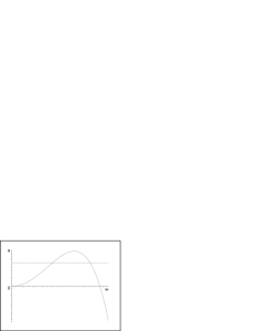
Figure 1: Vilenkin potential with $c=$const.

The maximum of the potential $U(a)$ is located at $a_{e}=\sqrt{3/2\Lambda}$ where $U(a_{e})=3c^{2}/(4\Lambda)$. The tunneling probability in WKB approximation can be estimated as

$$\emph{P}\sim\exp\left(-\frac{2c^{2}}{8\pi G\hbar}\int_{a^{\prime}_{i}}^{a_{i}}da\sqrt{U(a)-E}\right),$$ (1)

where $a^{\prime}_{i}<a_{i}$ are two turning points. The universe can start from $a=0$ singularity, expand to a maximum radius $a^{\prime}_{i}$ and then tunnel through the potential barrier to the regime of unbounded expansion with the semiclassical tunneling probability (1). Choosing $E=0$ one gets $a^{\prime}_{i}=0$ and $a_{i}=\sqrt{3/\Lambda}$. The integral in (1) can be calculated. The result can be written as

$$\emph{P}\sim\exp\left(-\frac{2c^{3}}{8\pi G\hbar\Lambda}\right).$$ (2)

For the probability to be of reasonable value, for example $\emph{P}=1/{\rm e}\sim 0.368$, one has to put $\Lambda\sim 0.3\times 10^{65}\,\,{\rm sm}^{-2}$ (see (2)). In other words, the $\Lambda$-term must be large. However, despite this problem, we does acquire one prise: Once nucleated, the universe immediately begins a de Sitter inflationary expansion. Therefore the tunneling wave function results in inflation. And the $\Lambda$-term problem, which arises in this approach is usually being gotten rid of via the anthropic principle.

Besides, there exists another way to estimate the (1). If the ”energy” is a random variable, one can consider P as a function from both $\Lambda$ and $E$. Then, assuming $E\sim U(a_{e})=3c^{2}/4\Lambda$ we quickly come to conclusion that the integral in (1) goes to zero and $\emph{P}\to 1$. Such universe don’t experience the inflation, therefore we are unable to classically solve the flatness and other problems. What can be said about $\Lambda$-term? For this to answer we’ll introduce the dimensionless variable $z_{0}={\tilde{a}}_{0}\sqrt{\Lambda}$ where ${\tilde{a}}_{0}=10^{28}$ sm is the widely accepted modern value of the scale factor. Assuming $H_{0}{\tilde{a}}_{0}=c$ ($H_{0}$ is the modern value of the Hubble parameter) allows to extract from the Einstein equation the biquadratic equation $4z_{0}^{4}-24z_{0}^{2}+9=0,$ therefore $z_{0}=2.366$ (the second positive root $z^{\prime}_{0}=0.634$ is less then $z_{e}=1.225$ which approximately corresponds to the initial value of the scale factor). Since the contribution of $\Lambda$ to the density is $\rho_{{}_{\Lambda}}=\Lambda c^{2}/8\pi G$, we can calculate the value $\Omega_{{}_{\Lambda}}=\rho_{{}_{\Lambda}}/\rho_{c}$, where $\rho_{c}=3H_{0}^{2}/8\pi G$ is the critical density. Upon doing this we get $\Omega_{{}_{\Lambda}}=z_{0}^{2}/3=1.866$ instead of observed $\Omega_{{}_{\Lambda}}=0.7$.

One can sum up all the premises as follows: (i) The semiclassical tunneling probability for the universe to nucleate into the inflation phase is very small for the small values of the $\Lambda$-term; (ii) the tunneling nucleation probability is large ($\emph{P}\sim 1$) for the universe which is filled with ”matter” (radiation ad hoc) - but with the total loss of inflation. Thus we have two different ways for the further inquiries: either to prefer the inflation and then go on with the anthropic principle or to find some kind of the inflation’s alternates.

Among such alternatives in physics nowadays one of the most interesting are certainly the cosmological models with varying speed of light (VSL) 1 , 2 (In fact, there are many articles about this matter. But we’d like to restrict ourselves to consider only these ones which has been used in this work.). In simplest case the speed of light $c=c(t)$ varies as some power of the expansion scale factor: $c(t)=sa^{n}(t)$, where constant $s>0$. Summarizing some of the promising positive features of these models: (a) It can solve the horizon and flatness problems if $n\leq n_{{}_{fl}}=-(3w+1)/2$; (b) in case of $n<n_{{}_{\Lambda}}=-3(w+1)/2$ the VSL models can solve the $\Lambda$-problem in a early universe while inflation models can’t handle it without the aid of the anthropic principle.

Of course, these VSL models result in some shortcomings and unusual (unphysical?) features as well 3 : (1) It is not clear how to solve the isotropy problem; (2) the quantum wavelengths of massive particle states and the radii of primordial black holes can grow sufficiently fast to exceed the scale of the particle horizon; (3) the entropy problem: Entropy can decrease with increasing time.

Keeping in mind all the above-mentioned problems we’d like, nevertheless, to consider VSL quantum cosmology. One of interesting observations is that the probability to find the finite universe short after it’s tunneling through the potential barrier is $\emph{P}\sim\exp(-\beta\Lambda^{\alpha})$ with $\alpha>0$ and $\beta>0$ for the special values of $n$ (see below). This means that the difference between P in VSL and usual quantum cosmology can be very significant.

The plan of the paper looks as follows: in the next Section we’ll consider the simplest VSL model: model of Albrecht-Magueijo-Barrow. In Sec. III we’ll study the case of nonsingular potentials $U(a)$ (the case A, with $n>n_{{}_{fl}}(w)$, see below). Although such a potentials are not fit to solve the cosmological problems in framework of classical VSL cosmology, they can be of interest in framework of quantum cosmology. In particular, as we will see, these potentials are easily result in $\Omega_{{}_{\Lambda}}\sim 0.7$. In Sec. IV and V we’ll study the models with singular potentials: the cases B ($n_{{}_{\Lambda}}(w)<n<n_{{}_{fl}}(w)$) and C ($n<n_{{}_{\Lambda}}(w)$). We’ll show that only potentials of the case B do have the ground state and therefore do have the physical meaning. Another interesting feature of the case B (Sec. V) is that it allows to solve the horizon and flatness problems without the aid of inflation. However, the $\Lambda$-problem can’t be solved in this case (on the classical level) but quantum cosmology predict $\Omega_{{}_{\Lambda}}\sim 0.7$ if ${\tilde{a}}_{0}=10^{28}$ sm with $\emph{P}\sim 1$! Unfortunately, in the case B we can’t obtain the universe with $w>1/9$ just after nucleation and this is probably the major shortcoming of the model. Despite the fact that the case C has no clear physical meaning it will be briefly considered in Sec. V, in hope that the string theory can breathe new life into these models (see the discussion in Sec. V). As an another reason can be named the interesting classical behavior of this model (see Appendix) while far from the singularity $a=0$. In Sec. VI we’ll consider two peculiar cases when $n=n_{{}_{fl}}$ and $n=n_{{}_{\Lambda}}$. It will be shown that the ground state is admitted for the first case only.

II Albrecht-Magueijo-Barrow VSL model

Lets start with the Friedmann and Raychaudhuri system of equations with $k=+1$ (we assume that $G$=const):

$$\begin{array}[]{cc}\displaystyle{\frac{\ddot{a}}{a}=-\frac{4\pi G}{3}\left(\rho+\frac{3p}{c^{2}}\right)+\frac{\Lambda c^{2}}{3},}\\ \\ \displaystyle{\left(\frac{\dot{a}}{a}\right)^{2}=\frac{8\pi G\rho}{3}-\left(\frac{c}{a}\right)^{2}+\frac{\Lambda c^{2}}{3},}\\ \\ \displaystyle{c=c_{0}\left(\frac{a}{a_{0}}\right)^{n}=sa^{n},\qquad p=wc^{2}\rho,}\end{array}$$ (3)

where $a=a(t)$ is the expansion scale factor of the Friedmann metric, $p$ is the fluid pressure, $\rho$ is the fluid density, $k$ is the curvature parameter, $\Lambda$ is the cosmological constant, $c_{0}$ is the modern value of the speed of light ($3\times 10^{10}$ sm/sec) and $a_{0}$ is the modern value of the scale factor. Usually, this value is estimated as $10^{28}$ sm. However, keeping in mind that the speed of light in our model is effectively decreasing, in fact we will choose $a_{0}=N\times 10^{28}$ sm with some $N>0$.

Using (3) we get

$$\dot{\rho}=-\frac{3\dot{a}}{a}\left(\rho+\frac{p}{c^{2}}\right)+\frac{{\dot{c}}c(3-a^{2}\Lambda)}{4\pi Ga^{2}}.$$ (4)

After the (4) solving we receive

$$\rho=\frac{M}{a^{3(w+1)}}+\frac{3s^{2}na^{2(n-1)}}{4\pi G(2n+3w+1)}-\frac{s^{2}n\Lambda a^{2n}}{4\pi G(2n+3w+3)},$$ (5)

where $M$ is a constant characterizing the amount of ”matter” with given $w$. It is clear from the (5) that the flatness problem can be solved in early universe by an interval of VSL evolution if $n<n_{{}_{fl}}(w)=-(1+3w)/2$, whereas the problem of $\Lambda$-term can be solved only if $n<n_{{}_{\Lambda}}(w)=n_{{}_{fl}}(w)-1=-3(w+1)/2$. The evolution equation for the scale factor $a$ (the second equation in system (3)) can be written as

$$P^{2}+U(a)=E,$$ (6)

where $P=-\dot{a}a^{-n_{{}_{fl}}(w)}$ is the momentum conjugate to $a$, $E=8\pi GM/3$ and

$$U(a)=s^{2}a^{2(n-n_{{}_{fl}}(w))}\left(\frac{3w+1}{2(n-n_{{}_{fl}}(w))}-\frac{\Lambda(w+1)a^{2}}{2(n-n_{{}_{\Lambda}}(w))}\right).$$ (7)

The expressions (5), (7) are valid if $n\neq n_{{}_{fl}}(w)$ and $n\neq n_{{}_{\Lambda}}(w)$. These cases will be considered separately.

The potential $U(a)$ is the ”quantum” potential from the Wheeler-DeWitt equation. To obtain the model with the nonzero quantum tunneling nucleation probability we should have the potential with the maximum. If we restrict ourselves to working only with the positive $\Lambda$ then the case $n_{{}_{fl}}(w)<0$ (i.e. $w>-1/3$) will get us one maximum at $a=a_{e}=\sqrt{(3w+1)/\Lambda(w+1)}$, where the function $U(a)$:

$$U(a_{e})=\frac{s^{2}(3w+1)}{2(n-n_{{}_{fl}}(w))(n-n_{{}_{\Lambda}}(w))}\left(\frac{3w+1}{\Lambda(w+1)}\right)^{n-n_{{}_{fl}}(w)}.$$ (8)

Next, as can be easily seen from the pictures, there exists three distinguishable cases: case (A) $n>n_{{}_{fl}}(w)$, see Fig. 2; case (B) $n_{{}_{\Lambda}}(w)<n<n_{{}_{fl}}(w)$, see Fig. 3; and case (C) $n<n_{{}_{\Lambda}}(w)$, see Fig.4.

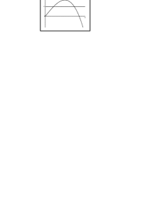
Figure 2: The case $n>n_{{}_{fl}}(w)$.

Figure 3: The case $n_{{}_{\Lambda}}(w)<n<n_{{}_{fl}}(w)$.

III The case A: $n>n_{{}_{fl}}(w)$

This case is seemingly the one that is favorable the least. In fact, since $n_{{}_{\Lambda}}(w)<n_{{}_{fl}}(w)$ then for $n>n_{{}_{fl}}(w)$ we can solve neither flatness nor $\Lambda$ problems while working in the framework of the Barrow approach. However, as we shall see, even such $n$ allows the $\Lambda$ problem to be solved - but solved in framework of quantum cosmology.

The equation (6) is quite similar to equation concerning particle of energy $E$ that is moving in potential (7), hence the universe in quantum cosmology can start at $a\sim 0$, expand to a maximum radius $a^{\prime}_{i}$ and then tunnel through the potential barrier to the regime of unbounded expansion with ”initial” value $a=a_{i}$. The semiclassical tunneling probability can be estimated as

$$\emph{P}\sim\exp\left(-2\int_{a^{\prime}_{i}}^{a_{i}}{\mid{\tilde{p}(a)}\mid}da\right),$$ (9)

with

$$\begin{array}[]{cc}{\mid{\tilde{p}(a)}\mid}=\left(8\pi G\hbar\right)^{(n_{{}_{fl}}(w)-1)/2}c^{(1-3n_{{}_{fl}}(w))/2}\mid P(a)\mid,\\ \\ \mid P(a)\mid=\sqrt{U(a)-E},\end{array}$$

where $E\leq U(a_{e})$. It is convenient to write $E=U(a_{e})\sin^{2}\theta$, with $0<\theta<\pi/2$. After calculation of this one we get

$$\begin{array}[]{cc}\displaystyle{\emph{P}\sim\exp\left(-\frac{\sqrt{2}}{\sqrt{(n-n_{{}_{fl}}(w))(n-n_{{}_{\Lambda}})}}\left(8\pi G\hbar\right)^{(n_{{}_{fl}}(w)-1)/2}s^{3(1-n_{{}_{fl}}(w))/2}\Lambda^{(3n+2)(n_{{}_{fl}}(w)-1)/4}W(w,\theta,n)\right)},\\ \\ \displaystyle{W(w,\theta,n)=\int_{z^{\prime}_{i}}^{z_{i}}\frac{dz}{z^{n(3n_{{}_{fl}}(w)-1)/2}}\sqrt{z^{2(n-n_{{}_{fl}}(w))}\left((n-n_{{}_{\Lambda}}(w))(3w+1)-(n-n_{{}_{fl}}(w))(w+1)z^{2}\right)-\kappa(w,\theta,n)},}\\ \\ \displaystyle{\kappa(w,\theta,n)=\frac{(3w+1)^{(n-n_{{}_{\Lambda}}(w))}\sin^{2}\theta}{(w+1)^{n-n_{{}_{fl}}(w)}}}\end{array}$$ (10)

where $z=a\sqrt{\Lambda}$, $z^{\prime}_{i}<z_{i}$ are the roots of expression under the integral. As we can see, for the $-(1+3w)/2<n<-2/3$ the probability P is increasing when $\Lambda\to 0$! In fact, the equations (6) apply the restriction on the values of $\Lambda$: the $\Lambda$ can’t be too small.

To show this, lets consider the case $w=1/3$ (radiation). If $n=0$ (i.e. $c$=const) the probability P does not vanish in the limit of $E\to 0$, when there is no radiation and the size of the initial universe shrinks to zero. In our situation this is not the case: the probability $\emph{P}=0$ at $E=0$. Therefore a newborn universe will inevitably be filled with the radiation.

In fact, for the small $E$ the (10) can be estimated as

$$\emph{P}=\exp\left(-\frac{s^{3}I(n,\theta)}{\pi G\hbar(4(n+1)^{3(n+1)/2})}\left(\frac{3(n+2)}{\Lambda}\right)^{(3n+2)/2}\right),$$

where

$$I(n,\theta)=\int_{x^{\prime}_{i}(n,\theta)}^{\pi/2}dx\left((\sin x)^{3n+1}-(\sin x)^{3(n+1)}\right),$$

with

$$x^{\prime}_{i}(n,\theta)=\arcsin\left((\sin\theta)^{1/(n+1)}\sqrt{\frac{n+1}{(n+2)^{(n+2)/(n+1)}}}\right).$$

Choosing $\theta=0.1$ and $n=-0.9$ one get $\emph{P}=\exp\left(-0.176\times 10^{149}\sqrt{\Lambda}\right)$, so this probability will be $\emph{P}\sim 1/{\rm e}\sim 0.37$ for the $\Lambda\sim 0.3\times 10^{-296}$ ${\rm sm}^{-2}$. But it is impossible due to the equation of motion (6). Choosing $E\sim 0$, we get

$$\Lambda=\frac{3(n+2)^{2}}{2(n+1)}\sim 18.15\,\,{\rm sm}^{-2},$$ (11)

for the $n=-0.9$, therefore $\emph{P}\sim\exp\left(-0.75\times 10^{149}\right)\sim 0$.

Thus, the probability P will be largest for $E\sim U(a_{e})$ (of course, if $E>U(a_{e})$ there is no quantum tunneling at all). So, we can choose $\theta\sim\pi/2$. In this case $z^{\prime}_{i}\sim z_{i}$ and the integral $W(w,\theta\sim\pi/2,n)\sim 0$, hence $\emph{P}\sim 1$. If, for example, $w=1/3$ then

$$\emph{P}\sim\exp\left(-\frac{3\sqrt{2}\epsilon^{2}s^{3}\Lambda^{-(3n+2)/2}}{8\pi G\hbar(n+1)(n+2)}\left(\frac{3}{2}\right)^{3n/2}\right),$$

where $\epsilon=\pi/2-\theta\ll 1$.

Lets consider the equation (6) with $w=1/3$. It leads us to equation

$$\begin{array}[]{cc}\displaystyle{(a{\dot{a}})^{2}+s^{2}a^{2(n+1)}\left(\frac{1}{n+1}-\frac{2\Lambda a^{2}}{3(n+2)}\right)=}\\ \\ \displaystyle{\frac{s^{2}}{(n+1)(n+2)}\left(\frac{3}{2\Lambda}\right)^{n+1}},\end{array}$$ (12)

with $\sin\theta\sim 1$. Substituting $a=a_{0}=Nc_{0}/H_{0}=N\times 10^{28}$ sm, where $H_{0}$ is the Hubble root we get

$$z_{0}+\frac{1}{(n+1)z_{0}^{n+1}}=\left(n+2\right)\left(N^{2}+\frac{1}{n+1}\right),$$ (13)

where $z_{0}=2\Lambda a_{0}^{2}/3$. The modern contribution of $\Lambda$ into the density is $\rho_{{}_{\Lambda}}=\Lambda c_{0}^{2}/(8\pi G)$. We can define the quantities $\Omega_{{}_{\Lambda}}=\rho_{{}_{\Lambda}}/\rho_{c}$, where $\rho_{c}=3H_{0}^{2}/(8\pi G)$ is the critical density and $\Omega_{{}_{R}}=\rho_{{}_{R}}/\rho_{c}$ where $\rho_{{}_{R}}$ is the radiation contribution. The simple calculation results in

$$\Omega_{{}_{\Lambda}}=\frac{z_{0}}{2N^{2}},\qquad\Omega_{{}_{R}}=\frac{z_{0}^{-(n+1)}}{(n+1)(n+2)N^{2}}.$$ (14)

Note, that in the beginning $z_{i}\sim 1$. Now we can solve (13) for any given $n$ (from the interval $-1<n<-2/3$) and $N$ in order to find $z_{0}$ which should be next substituted into the (14). The explicit results are presented in Table 1.

Table 1: The table of values of $z_{0}$, $\Omega_{{}_{\Lambda}}$ and $\Omega_{{}_{R}}$ for some of the $n$ from the interval $(-1;-2/3)$ and a few values of $N$. The most of values of $\Omega_{{}_{\Lambda}}$ are adjacent to the range $0.7$, and that is quite consistent with the observational data.

n	N	$z_{0}$	$\Omega_{{}_{\Lambda}}$	$\Omega_{{}_{R}}$
-0.9	1	3.2	1.6	8.09
-0.9	2	7.19	0.899	1.87
-0.9	3	13.7	0.732	0.78
-0.9	4	21.23	0.664	0.42
-0.9	5	31.42	0.628	0.25
-0.9	10	114.78	0.574	0.06
-0.9	100	1.1$\times 10^{4}$	0.55	0.36$\times 10^{-3}$
-0.8	1	3.25	1.63	3.29
-0.8	2	7.45	0.93	0.7
-0.8	3	13.84	0.77	0.27
-0.8	4	22.52	0.7	0.14
-0.8	5	33.52	0.67	0.08
-0.8	10	124.09	0.62	0.02
-0.8	100	1.2$\times 10^{4}$	0.6	6$\times 10^{-5}$
-0.7	1	3.3	1.65	1.79
-0.7	2	7.73	0.97	0.35
-0.7	3	14.54	0.81	0.13
-0.7	4	23.85	0.75	0.06
-0.7	5	35.69	0.71	0.04
-0.7	10	133.57	0.67	6$\times 10^{-3}$
-0.7	100	1.3$\times 10^{4}$	0.65	6$\times 10^{-5}$

For all the cases the value $\Lambda\sim 10^{-55}$ ${\rm sm}^{-2}$, which is much less then (11).

As we can see, the values of $\Omega_{{}_{\Lambda}}$ lies in most near the range $0.7$. And this is in quite good consent with the observational data.

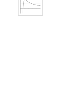
Figure 4: The case $n<n_{{}_{\Lambda}}(w)$.

IV An existence of ground states for singular potentials (The case B)

It is interesting to ask: what can be said about the value of $U(a)$ when $a=0$? It is easy to see from (7), that (depending on the values of $w$ and $n<0$), the potential $U(a)$ can take on one of two different values: either $0$ (Fig. 2) or $-\infty$, (Fig. 3 and Fig. 4). Since we consider only $w>-1/3$ values, the second case is valid for every $n$ satisfying the inequality $n<n_{{}_{fl}}(w)<0$. Thus, it leads us to another question: what can be the possible meaning of the potential which at $a\to 0$ is unbounded from below? It seems that such universe is able to just roll down towards small values of $a$ (where the potential is tending to minus infinity) instead of any tunneling to large values.

This situation can in fact be alleviated if the considered potential $U(a)$ has the ground state. Indeed, one can imagine the fictitious particle with some energy and coordinate $a(t)$ in the potentials (7) (see Fig.3 and Fig. 4) rolling down towards small values of $a$. The main problem is: whether the quantum mechanical energy spectrum of $U(A)$ is unbounded below? If not, then it does admits the ground state and hence can have the physical meaning.

To find such a potential lets suppose that our fictitious particle is located in a small region $a$ near the singularity $a=0$, with the momentum $P$. One can use the Heisenberg uncertainty relation as

$$P\,a\sim\left(8\pi G\hbar\right)^{(1-n_{{}_{fl}}(w))/2}c^{(3n_{{}_{fl}}(w)-1)/2}.$$ (15)

Using (15), and (3) (or (6)) one get for the $a\to 0$

$$\begin{array}[]{cc}\displaystyle{E=P^{2}+U(a)\to}\\ \\ \displaystyle{\to\frac{Z^{2}}{a^{2-n(3n_{{}_{fl}}(w)-1)}}+\frac{s^{2}n_{{}_{fl}}(w)}{(n_{{}_{fl}}(w)-n)a^{2(n_{{}_{fl}}(w)-n)}}},\end{array}$$

where $Z^{2}=\left(8\pi G\hbar\right)^{1-n_{{}_{fl}}}s^{3n_{{}_{fl}}-1}$, and

$$n<n_{{}_{fl}}(w)<0.$$ (16)

Therefore the energy spectrum will be bounded below if

$$\left(3n+2\right)\left(n_{{}_{fl}}(w)-1\right)<0.$$ (17)

and (16) are valid. This situation is represented graphically on the Fig. 5.

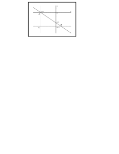
Figure 5: The ground state exists for $w$ and $n$ from the interior of the triangle ABC.

It is easy to see that the conditions of ground state existence can be satisfied by case B only (see Fig. 3). It is also important to note that the left side of the (17) (accurate to the coefficient $1/4$) is actually the power of $\Lambda$ in the probability (10)^[1] . But doesn’t it means that those sensible potentials which are unbounded from below at $a\to 0$ all result in semiclassical tunneling nucleation probability, strongly suppressed for small values of $\Lambda$, just as in the models with $c$=const? In reality, the through examination of the model shows that the situation is much better than it first looks. As we shall see, the universes which have nucleated with the probability $\emph{P}\sim 1$ would have the $\Omega_{{}_{\Lambda}}\sim 0.7$ for the $N\sim 1$!

To show this, lets choose $w=0$ (unfortunately, the case $w=1/3$ is inaccessible for the case B, since the maximum value is $w=1/9$, see Fig. 5) and $E=U(a_{e})\cosh\theta$. It is obvious that $\emph{P}\sim 1$ for sufficiently small $\theta$. Choosing $\theta\to 0$ one can estimate the probability as

$$\emph{P}\sim\exp\left(\frac{4s^{9/4}\theta^{2}}{(2n+1)(2n+3)\left[8\pi G\hbar\Lambda^{(3n+2)/2}\right]^{3/4}}\right).$$

Now, lets consider the equation (6) with $w=0$. We get

$$N^{2}+\frac{1}{2n+1}=\frac{1}{2n+1}\left(z_{0}^{2}+\frac{2}{(2n+3)z_{0}^{2n+1}}\right),$$ (18)

where

$$z_{0}=\frac{Nc_{0}\sqrt{\Lambda}}{H_{0}}=a_{0}\sqrt{\Lambda}.$$

The equation (18) is the analog of the (13) for the case $w=0$. Finally, $\Omega_{{}_{\Lambda}}=z_{0}^{2}/(3N^{2})$. It is necessary to remember that for case $w=0$ we have

$$-\frac{2}{3}<n<-\frac{1}{2}.$$

Since $2n+1<0$ the value $N$ is bounded above $N<N_{max}(n)$ (see (18)). For example $N_{max}(-0.65)=1.826$, $N_{max}(-0.6)=2.236$, $N_{max}(-0.55)=3.162$. Solving (18) for given $n$ and $N$ one get $z_{0}$ and $\Omega_{{}_{\Lambda}}$ (see Tabl. 2)

Table 2: A table of values of $z_{0}$ and $\Omega_{{}_{\Lambda}}$ for some $n$ from the interval $(-2/3;-1/2)$ and a few values of $N$.

n	N	$z_{0}$	$\Omega_{{}_{\Lambda}}$
-0.65	1	1.416	0.669
-0.65	1.4	1.298	0.286
-0.65	1.8	1.115	0.128
-0.6	1	1.411	0.663
-0.6	1.5	1.313	0.255
-0.6	2	1.16	0.112
-0.55	1	1.411	0.663
-0.55	2	1.296	0.14
-0.55	3	1.077	0.043

It is really astonishing that case $N=1$ (i.e. $a_{0}=10^{28}$ sm) results in $\Omega_{{}_{\Lambda}}\sim 0.7$, this result being strikingly consent with the observational data. Besides, one can choose to put $\Omega_{{}_{\Lambda}}=0.7$ instead and then solve (18) to find $N(n)$. As a result one will get $N(-0.65)=0.98$, $N(-0.6)=0.976$, $N(-0.55)=0.975$. Thus, in contrast to the case A, the universe bearing a maximum probability of nucleation via quantum tunneling and with the modern value of scale factor near $10^{28}$ sm must has $\Omega_{{}_{\Lambda}}\sim 0.7$.

In conclusion to this section, we should discuss one point of the model, that can be somehow of disturbance for us. The problem that is at issue arises from the fact, that $\emph{P}\sim 1$ if $\theta\sim 0$, i.e. $E\sim U(a_{e})<0$. This means that the constant characterizing the amount of ”matter” with $w=0$ (”the mass of dust”) is negative. We have full right to ask whether such statement is physically consistent. To be more exact, one can be afraid of facing the violation of the weak energy condition $\rho>0$, $\rho+p/c^{2}>0$. Fortunately, in case of the considered example such misgivings tends to be groundless. Using (4) we can get

$$\rho_{0}=\frac{c_{0}^{2}\Lambda\left(3z_{0}^{-2n}+6n^{2}z_{0}+9nz_{0}-n(2n+1)z_{0}^{3}\right)}{4\pi G(2n+1)(2n+3)z_{0}^{3}},$$

where $\rho_{0}$ is a modern value of total density. Using the Tabl. 2 one can verify that for those values of $n$ and $w$ that are of interest for us $\rho_{0}>0$.

V The case C

As we have shown, the conditions of the ground state existence for singular at $a\to 0$ potentials can only be satisfied for potentials from the case B. With this in account, we can come to a very uncomfortable conclusion that the case C (and a rest of case B) has no any physical meaning.

However, in order to make these potentials physical, there still exists but one loophole. This loophole follows from a strings theory prediction that states the existence of $a_{min}$ – the minimal spatial scale. Due to the strings theory, there is no sense in considering the physics at $a<a_{min}$. If this is true, then we should not deny the possibility of potentials $U(a)$ with $n<n_{{}_{fl}}(w)<0$ to be the physical potentials with existing ground state - this, of course, being just a speculation. Keeping this in mind, let us now consider the model with $w=1/3$, $n_{{}_{fl}}=-1$, $n=-1-m$, and $m>0$.

In this case the semiclassical tunneling probability has a form $\emph{P}\sim\exp(-S)$ with

$$S=\frac{s^{3}\Lambda^{(3m+4)/2}}{4\pi G\hbar 3^{(m+1)/2}\sqrt{m(m+1)}}\int_{z^{\prime}_{i}}^{z_{i}}\frac{dz\sqrt{F_{m}(z,\theta)}}{z^{3m+5}},$$

where

$$F_{m}(z,\theta)=-2^{m+1}\sin^{2}\theta\,z^{2(m+1)}+2\times 3^{m}(m+1)z^{2}-m3^{m+1},$$

$z$ is a dimensionless quantity and $z^{\prime}_{i}$, $z_{i}$ are the turning points, i.e. two real positive solutions of the equation $F_{m}(z,\theta)=0$ for given $\theta$ (it is easy to see that the equation $F_{m}(z,\theta)=0$ does have two such solutions at $0<\theta<\pi/2$).

If $m$ is the whole number then the expression for the P has more simple form. For example

$$\emph{P}_{1}\sim\exp\left(-\frac{s^{3}\Lambda^{7/2}\sin\theta}{6\pi G\hbar\sqrt{2}}\int_{z^{\prime}_{i}}^{z_{i}}\frac{dz}{z^{8}}\sqrt{(z^{2}-{z^{\prime}_{i}}^{2})(z_{i}^{2}-z^{2})}\right),$$

with

$$z^{\prime}_{i}=\frac{\sqrt{3}}{2\cos(\theta/2)},\qquad z^{\prime}_{i}=\frac{\sqrt{3}}{2\sin(\theta/2)}.$$

This expression can be calculated exactly:

$$\emph{P}_{1}\sim\exp\left(-\frac{s^{3}\Lambda^{7/2}\sin\theta J(\theta)}{6\sqrt{2}\pi G\hbar}\right),\qquad J(\theta)=\frac{1}{105}\left(\frac{2\sin(\theta/2)}{\sqrt{3}}\right)^{5}\left[\Delta(\theta)\Pi\left(\mu^{2};\frac{\pi}{2}{\backslash}\arcsin\mu\right)-2\left(2\lambda^{4}-\lambda^{2}+2\right)\textrm{K}(\mu^{2})\right],$$

with $\mu^{2}=\cos\theta/\cos^{2}(\theta/2)$, $\lambda=\cot(\theta/2)$, $\Delta(\theta)=(8\lambda^{4}-13\lambda^{2}+8)/\cos^{2}(\theta/2)$, $\Pi$ and K are complete elliptic integrals of the first and third kinds correspondingly (see 8 )

Similarly, $\emph{P}_{2}\sim\exp(-S_{2})$, with

$$S=\frac{s^{3}\Lambda^{5}\sin\theta}{18\pi G\hbar}\int_{z^{\prime}_{i}}^{z_{i}}\frac{dz}{z^{11}}\sqrt{(z^{2}+z_{1}^{2})(z^{2}-{z^{\prime}_{i}}^{2})(z_{i}^{2}-z^{2})},$$

where

$$\begin{array}[]{cc}\displaystyle{z_{1}=\sqrt{\frac{3}{\sin\theta}\cos\left(\frac{\theta}{3}-\frac{\pi}{6}\right)},\qquad z^{\prime}_{i}=\sqrt{\frac{3}{\sin\theta}\sin\frac{\theta}{3}},}\\ \\ \displaystyle{z_{i}=\sqrt{\frac{3}{\sin\theta}\cos\left(\frac{\theta}{3}+\frac{\pi}{6}\right)}},\end{array}$$

and so on.

Since the case C is still questionable, we will restrict ourselves to the examples above. Note, however, that such models can be quite interesting in classical (non-quantum) cosmology (see Appendix). Another example of such calculations can be found in Yurov .

VI Peculiar cases

If $n=-(3w+1)/2$ then

$$U(a)=s^{2}\left(1+(3w+1)\log(\lambda\sqrt{\Lambda}a)-\frac{\Lambda(1+w)a^{2}}{2}\right),$$ (19)

with $P=-{\dot{a}}/a^{n}$, and some $\lambda$, that is dimensionless.

Similarly, if $n=-3(w+1)/2$ the potential $U(a)$ takes form:

$$U(a)=-s^{2}\left(\frac{3w+1}{2a^{2}}+\Lambda\left(\frac{1}{3}+(w+1)\log(\lambda\sqrt{\Lambda}a)\right)\right),$$ (20)

with $P=-{\dot{a}}/a^{n+1}$. Now we should study these potentials concerning the existence of the ground state. The calculations result in following conclusions: The potential (19) does have a ground state for the $-1/3<w<1/9$ whereas the potential (20) is missing it wholly. Thus, we’ll further consider only the case (19). This potential has one maximum at $a_{e}=\sqrt{(3w+1)/(1+w)\Lambda}$ and

$$U(a_{e})=\frac{s^{2}}{2}\left(1-3w+(1+3w)\log\frac{\lambda^{2}(1+3w)}{1+w}\right).$$

Substituting $E\sim U(a_{e})$ (in order to obtain $\emph{P}\sim 1$) into the (6) we get the following equation

$$(1+w)z_{0}^{2}-(1+3w)\log\frac{z_{0}^{2}}{z_{e}^{2}}=2N^{2}+1+3w,$$ (21)

where $z_{0}=\sqrt{\Lambda}N\times 10^{28}$, $z_{e}=\sqrt{(3w+1)/(w+1)}$. The value of $a_{e}=z_{e}/\sqrt{\Lambda}$ is the initial value of scale factor (after the tunneling) to high precisions. Now we can solve (21) for given $w$ and $N$. The results of such a calculation are presented in Tabl. 3.

Table 3: A table of values of $z_{0}/z_{e}$ and $\Omega_{{}_{\Lambda}}$ for some $w$ from the interval $(-1/3;1/9)$ and a few values of $N$. All calculations are done for potential (19).

w	N	$z_{0}/z_{e}$	$\Omega_{{}_{\Lambda}}$
-0.3	1	4.918	1.152
-0.3	5	22.52	0.966
-0.3	10	44.89	0.957
-0.3	100	447.2	0.952
-0.2	1	2.844	1.349
-0.2	5	11.44	0.872
-0.2	10	22.52	0.845
-0.2	100	223.6	0.834
-0.1	1	2.361	1.446
-0.1	5	8.762	0.796
-0.1	10	17.1	0.758
-0.1	100	169	0.741
0	1	2.123	1.502
0	5	7.417	0.733
0	10	14.36	0.688
0	100	141.5	0.677
0.1	1	1.98	1.536
0.1	5	6.57	0.681
0.1	10	12.7	0.63
0.1	100	124.1	0.607

We can see that $\Omega_{{}_{\Lambda}}\sim 0.7$ when $w=-0.1$, $N>100$; $w=0$, $N\sim 5-10$; $w=0.1$, $N\sim 3-5$.

VII Conclusion

As we have seen, the semiclassical tunneling nucleation probability in the VSL quantum cosmology is really different from the one in the quantum cosmology with $c$=const. The most interesting distinction lies in capability of the VSL model to provide via the quantum nucleation the flat universe with $\emph{P}\sim 1$ and the horizon problem solved. Moreover, the VSL model here is the only tool of obtaining the solution of both the flatness and horizon problems without the aid of inflation, since it is not quite clear how to obtain the inflation in universe where the ”matter” energy density is greatly exceeding those of the vacuum. And as the additional prize of the model we get $\Omega_{{}_{\Lambda}}\sim 0.7$ without much of an effort.

However, it would be too prematurely to say that VSL quantum cosmology is indeed the actual panacea for the $\Lambda$-mystery and another cosmological problems as well. First of all, as we have seen, the case B, that is the most promising one, fails to describe quantum tunneling into the classical state with $w=1/3$. The validity of the WKB wave function in general is the model’s second problem. And also there are the omitted pre-exponential factors which can be nevertheless essential for the analysis of the vicinities of the turning points.

But, even with this in account, the shown difference of P in the VSL and the usual quantum cosmology seems very interesting and also very significant.

Appendix A

Lets take $w=1/3$, $n=-2-m$, for the $m\geq 0$. Surely, in this case we have no ground state. In spite of this sad circumstance we’ll still consider this model far from the $a=0$ where this model looks as a wholly satisfactory one.

Substitution of the (5) into the first equation of system (3) yields

$${\ddot{a}}=\frac{1}{a^{3}}\left[-E+\frac{s^{2}}{a^{2m}}\left(-\frac{m+2}{(m+1)a^{2}}+\frac{2(m+1)\Lambda}{3m}\right)\right].$$ (22)

Thus we have the following situations:
1. If

$$0<a^{2}\ll\frac{3m(m+2)}{2\Lambda(m+1)^{2}},$$

then the curvature term is the dominating one and ${\ddot{a}}<0$.
2. If

$$\frac{3m(m+2)}{2\Lambda(m+1)^{2}}\ll a^{2}\ll{\tilde{a}}^{2}\equiv\left(\frac{2s^{2}(m+1)\Lambda}{3mE}\right)^{1/m},$$ (23)

then the dominating term is $\Lambda$-term and $\ddot{a}>0$ during this time.
3. If

$$a^{2}\gg\left(\frac{2s^{2}(m+1)\Lambda}{3mE}\right)^{1/m},$$

then the radiation term is the dominating one and ${\ddot{a}}<0$.

There are two way to interpret the region (A2). The first way is to conclude that we have cosmological inflation in early universe. This is possible when $0<m\ll 1$. In this case we can evaluate the number of e-foldings $\Delta N$ during the region (A2) as

$$\log m\sim-2m\Delta N,\qquad\Lambda\gg\frac{3Em}{2s^{2}}\sim\frac{3Em}{2c_{0}^{2}a_{0}^{4}}.$$ (24)

If $\Delta N\sim 60$ then $m\sim 0.029$; if $\Delta N\sim 100$ then $m\sim 0.0197$. To evaluate $E$ one can use the well-known expression for the Friedmann integrals Cher ,

$$A(w)=\left[\left(\frac{1+3w}{2}\right)^{2}E\right]^{1/(1+3w)}.$$

Since $A(1/3)=3\times 10^{36}$ ${\rm sm}^{2}/{\rm sec}$, we get $E=0.9\times 10^{73}$ ${\rm sm}^{4}/{{\rm sec}^{2}}$. The substitution of $A(1/3)$ into the (24) results in

$$\Lambda\gg 0.435\times 10^{-61}\,\,{\rm sm}^{-2},\qquad\Lambda\gg 0.296\times 10^{-61}\,\,{\rm sm}^{-2},$$

for the $\Delta N=60$ and $\Delta N=100$.

But do we really need inflation in the VSL models? The question is not quite clear. On the one hand, VSL models can solve fundamental cosmological problems (horizon and flatness problems) without inflation - and what is more, these models can solve $\Lambda$-problem whereas inflations can’t do it without the anthropic principle. On the other hand, the simplest case of VSL cosmological models, which is the subject of this article, is facing with the isotropy problem 3 . But, as we have seen, VSL model results in inflation with exit naturally so it will be incorrect to oppose VSL models and the inflation.

Another way to interpret the region (23) is to identify this region with the modern acceleration of universe. This is possible if $m$ is sufficiently large. Let us make a crude guess. According to modern observations we can write ${\ddot{a}_{0}}/a_{0}=5.6\pi G\rho_{c}/3$ where $\rho_{c}=10^{-29}$ ${\rm{gramme/sm^{3}}}$. If the modern value of $a_{0}\sim{\tilde{a}}$ (see the inequality (23)) then

$$\Lambda=\frac{3mE}{3c_{0}^{2}(m+1)a^{4}_{0}}.$$ (25)

From the (22) we have

$$\ddot{a}_{0}\sim\frac{2(m+1)\Lambda s^{2}}{3ma^{2m+3}_{0}}$$

if the $\Lambda$-term is dominating one. Substituting (25) gets us

$$\Omega_{{}_{\Lambda}}=\frac{\Lambda c_{0}^{2}}{8\pi G\rho_{c}}\sim\frac{0.35m}{m+1},\qquad a_{0}\sim{}^{4}\sqrt{\frac{3E}{5.6\pi G\rho_{c}}}.$$

Thus, if $m\gg 1$ then $\Omega_{{}_{\Lambda}}\sim 0.35$, $\Lambda\sim 0.2\times 10^{-56}$ ${\rm sm}^{-2}$, $a_{0}\sim 10^{27}$ sm. And these values are seems to be quite reasonable.

References

1. J.B. Hartle and S.W. Hawking, Phys. Rev. D28, 2960 (1983).
2. A.D. Linde, Lett. Nuovo Cimento 39, 401 (1984).
3. A. Vilenkin, Phys. Rev. D30, 509 (1984); A. Vilenkin, Phys. Rev. D33, 3560 (1986).
4. A. Vilenkin, gr-qc/0204061.
5. A. Albrecht and J. Magueijo, Phys. Rev. D 59, 043516 (1999).
6. J.D. Barrow, Phys. Rev. D 59, 043515 (1999).
7. J.D. Barrow, gr-qc/0211074.
8. M. Abramowitz and I. Stegun, “Handbook of Mathematical Functions.” Dover Publications Inc., New York, 1046 p., (1965).
9. A.V. Yurov and V.A. Yurov, [hep-th/0410231].
10. A.D. Chernin, Nature, 220, 250 (1968); A.D. Chernin, astro-ph/0101532.
11. T.Harko , H.Q.Lu , M.K.Mak and K.S.Cheng, Europhys.Lett., 49 (6), 814 (2000).