Statistics of $M$ theory Vacua.


B.S. Acharya^a , F. Denef^b and R. Valandro<sup>c

a</sup> Abdus Salam ICTP, Strada Costiera 11,
34014 Trieste, ITALIA
^b New High Energy Theory Center,
Rutgers University, Piscataway.
NJ 08554 USA
^c International School for Advanced Studies (SISSA/ISAS),
Via Beirut 2-4, 34014 Trieste, ITALIA

Abstract

We study the vacuum statistics of ensembles of $M$ theory compactifications on $G_{2}$ holonomy manifolds with fluxes, and of ensembles of Freund-Rubin vacua. We discuss similarities and differences between these and Type IIB flux landscapes. For the $G_{2}$ ensembles, we find that large volumes are strongly suppressed, and for both, unlike the IIB case, the distribution of cosmological constants is non-uniform. We also argue that these ensembles typically have exponentially more non-supersymmetric than supersymmetric vacua, and show that supersymmetry is virtually always broken at a high scale.

1 Introduction and Summary

String theory has long held the promise to provide us with a complete and final description of the laws of physics in our universe. Yet from the start it was clear that the theory allows many vacua we clearly do not live in — ten dimensional Minkowski space being the simplest example. Over the past two decades, the existence of an infinite set of distinct stable vacua in which we obviously do not reside was firmly established. For some of those, such as Type IIB string theory on ${\rm AdS}_{5}\times S^{5}$ with flux, we even have complete nonperturbative descriptions. The vast majority of these well understood vacua have unbroken supersymmetry and come either with massless scalars or a negative cosmological constant of the order of the KK scale, all properties we certainly do not observe. Moreover, even though constructing vacua with light charged particles is fairly straightforward, typically such vacua are very different from the standard model at low energies.

The implicit assumption, of course, was that at least one vacuum should exist with broken supersymmetry, with just the standard model at low energies, and a couple of rather astonishing hierarchies between the cosmological, electroweak and Planck scales. One could hope that some deep dynamical mechanism uniquely selects such a vacuum, with all its peculiarities, rather than one from the enormous set of consistent vacua already firmly established, or from the presumably even much more enormous set of vacua that do not satisfy the rather artificial constraint of being under our full computational control at the present stage of theoretical development. Thus far however, no indication whatsoever has emerged that this is indeed the case, and anyway there is no realistic hope that the “correct” vacuum could be computed from such hypothetical dynamical principles with what we currently know about string theory.

It thus seems more modest and productive to follow the historically successful approach of trying to construct models that are compatible both with experimental and theoretical constraints. Whilst progress is continually being made in the program of constructing string theory vacua which meet rough observational requirements such as obtaining the standard model spectrum at low energies, no massless scalars or a small positive cosmological constant, no explicit model has been constructed combining all of these features. Clearly though, the examples studied thus far represent only an infinitesimal part of the tip of the iceberg, as computational complexity quickly turns into a major obstacle. The iceberg in question has been called the string theory landscape, and the problem we face is to find places in this landscape that could describe our universe.

Before embarking on this program however, it would evidently be useful to know what our chances of success are. For example it could save us a lot of time and effort if we managed to exclude large regions of the landscape, or more precisely large classes of models, before attempting to find realistic string theory vacua there. Traditionally the approach has been to focus on the most easily controllable constraints such as light charged particle spectra, while ignoring issues such as moduli stabilization, supersymmetry breaking or the cosmological constant. However these constraints are equally important, and it would be very useful to estimate how much they reduce the set of possibilities. For instance, one could propose a certain compactification with just the standard model living on a set of branes, and with very large compactification volume to explain the hierarchy between the electroweak and Planck scales, along the lines of [1]. This would already seem like a considerable triumph. A courageous model builder might then go on and try to turn on various fluxes to stabilize all moduli within the required region of moduli space, following the scenario of [2] or [3]. But this theorist will plausibly end his project disillusioned, finding not a single vacuum with volume even remotely close to what is required for this model to work. Indeed, it is generally true in these scenarios that flux vacua rapidly become more scarce at larger compactification volumes, and completely cease to exist even at very modest sizes. Clearly, our model builder would have benefited greatly from some simple estimates of distributions of actual vacua over the parameter space of the model.

In [4], it was furthermore pointed out that a sufficiently fine “discretuum” of string theory vacua could accommodate an extremely small but nonzero cosmological constant. To find out whether this idea can be realized in a given ensemble of vacua, and more generally to analyze how strongly constraints on various parameters reduce the number of possibilities within a given class of models (possibly down to zero as in the example above), one would like to have an estimate of how many vacua with certain properties lie in a given region of the landscape. In other words, one needs to study the statistics of vacua in this region (where “statistics” does not refer to any probability measure, but simply to number distributions on parameter space). This program was initiated in [5] and has been developed, thus far mainly for Type IIB flux vacua, in [6, 7, 8, 9, 10, 11, 12, 13, 14, 15, 16]. A number of ideas on the important question of distributions of supersymmetry breaking scales were proposed in [17, 18, 19], and subsequently significantly qualified in [20]. Further considerations on this topic have been made from an effective field theory point of view in [21, 22]. Distributions of gauge groups and particle spectra were studied in detail in [23, 24]. A number of effective field theory models of the landscape and phenomenological consequences have been analyzed in [25, 26, 27, 28], and some aspects of the statistics of string vacua beyond critical theories have been explored in [29]. Finally, more critical viewpoints of the string landscape have appeared in [30, 31].

One class of vacua that are interesting from a phenomenological point of view are $M$ theory compactifications on manifolds of $G_{2}$ holonomy [32]. Because of string duality there are presumably at least as many such vacua as there are heterotic string vacua on Calabi-Yau threefolds. It is thus important to get an idea of how moduli, compactification volumes, cosmological constants and supersymmetry breaking scales are distributed within this class of models. This will be the subject of the main part of this paper.

Although guidance for model building already provides enough motivation for statistical studies, one could be more ambitious and try to infer general properties of distributions of string theory vacua from statistical analysis of particular regions of the landscape combined with genericity arguments. To get some confidence in such results, one would need to explore and compare as many regions of the landscape as possible. Thus far however, only Type IIB flux vacua have been analyzed in detail. Because of string duality, one might optimistically hope that such IIB flux vacua could be representative — in the sense that they constitute a significant fraction of all string vacua, perhaps constrained to have some additional properties such as supersymmetry in the UV. However, it should be noted that the studies in [6] - [16] are limited to vacua described as Calabi-Yau orientifolds at moderately large volume and moderately weak string coupling, and strictly speaking these represent only a corner of the string theory landscape. In principle, distributions of observables could change dramatically as one explores different regions of the landscape. It was suggested in [33] that the set of four dimensional string and $M$ theory vacua with ${\cal N}=1$ or no supersymmetry is a disconnected space whose different components represent qualitatively different low energy physics, and this could translate into very different statistical properties. This gives us additional motivation to study the statistics of $G_{2}$ vacua and compare to the IIB case.

Another branch of the landscape whose statistical analysis we initiate here is the set of Freund-Rubin vacua [34], i.e. $M$ theory compactifications on Einstein manifolds with positive scalar curvature. Their properties are quite different from more familiar compactifications on special holonomy manifolds, and as we will see, this is reflected in their vacuum distributions which are very different as well.

Finally, one could take things one step further and altogether discard the idea that some mysterious dynamical mechanism has uniquely selected our vacuum and in particular picked the bizarre and exceedingly nongeneric scale hierarchies which just happen to be also necessary to make structure formation and atoms other than hydrogen or helium possible [35, 36, 37, 38, 28]. Instead, one could start with the hypothesis that a “multiverse” exists in which a huge number of vacua is actually realized, and in particular that we observe ourselves to be in a vacuum with such large scale hierarchies simply because this is needed for structure and atoms, and therefore observers, to exist. To make direct predictions from just string theory in such a framework, one would need to know the probability measure on at least the part of the landscape compatible with a number of basic requirements. There is no established way of computing these probabilities at this time, but as an additional working hypothesis one might assign for example in a given ensemble of flux vacua approximately the same probability to every choice of flux. One could refine this by restricting this equal probability postulate to subsets of vacua with fixed values of parameters relevant for cosmology, such as the vacuum energy, as one does for microstates with equal energy in the microcanonical ensemble of statistical mechanics. Different choices of these relevant parameters might then be weighted by cosmological considerations (up to the extent that this is needed, as some will be effectively fixed by environmental requirements). Under such hypotheses, suitable number distributions can be interpreted as probability distributions, and one can test the hypotheses that went in by Bayesian inference.

It should be emphasized that this framework is significantly more predictive than the traditional model building approach of simply considering any model compatible with current observations. Under these simple hypotheses, the landscape picture together with a few rough environmental principles gives a new notion of naturalness for effective field theories, which translates into a set of rules for model building. This turns out to lead to very distinct models which do not need contrived engineering to fit known data, and which moreover give very specific predictions, including many unambiguous signatures at LHC [38, 39, 28].

More theoretical data on number distributions obtained from string theory would obviously be very useful to make further progress in this area, and although as we discussed there are several other motivations for studying the statistics of string and $M$ theory vacua, we consider this to be a very important one.

The analysis of the $M$ theory vacua we study in this paper is somewhat technical, so for the ease of the reader, in the remainder of this introduction, after a brief review of the Type IIB flux landscape, we present a summary of our main results.

1.1 Review of Type IIB statistics

For comparison, let us briefly review what is known about the statistics of IIB flux vacua of Calabi-Yau orientifolds. There is a natural splitting of Kähler and complex structure moduli in this context. Turning on flux induces a superpotential [40] which only depends on the complex structure moduli. In suitable circumstances the Kähler moduli can be stabilized by nonperturbative effects, along the lines of [2, 41]. It is reasonable to ignore the Kähler moduli altogether as far as vacuum statistics is concerned, because (1) the main contribution to vacuum multiplicities comes from the huge number of different fluxes, (2) at sufficiently large volume the Kähler moduli do not influence the positions in complex structure moduli space significantly, and (3) practically, the Kähler sector of is less under control and more difficult to treat systematically.

The results for the distributions of moduli, cosmlogical constants, volumes and supersymmetry breaking scales for IIB flux vacua are roughly as follows.

1. The number of supersymmetric vacua in a region ${\cal R}$ of complex structure moduli space is estimated by [6]

   $${\cal N}_{\rm vac}({\cal R})=\frac{(2\sqrt{\pi}L)^{b_{3}}}{b_{3}!}\int_{\cal R}\det(R+\omega{\bf 1})$$ (1.1)

   where $L$ is the induced D3 brane charge by O3, O7 and D7 branes, $b_{3}$ is the third Betti number of the Calabi-Yau manifold, $R$ is the curvature form on the moduli space and $\omega$ the Kähler form. Actually this expression gives an index rather than an absolute number — it counts vacua with signs, so it is strictly speaking a lower bound. Essentially this expression implies that vacua are uniformly distributed over moduli space, except when the curvature part becomes important, which is the case near conifold degenerations. The above result was verified by Monte Carlo experiments in [10, 14].

2. The cosmological constant for supersymmetric vacua is $\Lambda=-3e^{K}|W|^{2}$. Its distribution for values much smaller than the string scale was found in [9] to be essentially uniform, i.e.

   $$d{\cal N}\sim{\cal N}_{\rm tot}\,d\Lambda.$$ (1.2)

   Here ${\cal N}_{\rm tot}\sim L^{b_{3}}/b_{3}!$ is the total number of flux vacua.

3. The compactification volume $V$ is stabilized by nonperturbative D3-instanton effects and/or gaugino condensates, both of which give contributions $\sim e^{-cV^{2/3}}$ to the superpotential, where $c<1$ decreases when $b_{3}$ increases. In the scenario of [2], these have to balance against the contribution $W_{0}$ from the fluxes. That is, at sufficiently large $V$ (or equivalently sufficiently small $W_{0}$), $e^{-cV^{2/3}}\sim W_{0}$. Since $|W_{0}|^{2}\sim\Lambda$ is uniformly distributed according to (1.2), this gives the volume distribution

   $$d{\cal N}\sim{\cal N}_{\rm tot}\,e^{-2cV^{2/3}}d(V^{2/3}).$$ (1.3)

   Large volumes are therefore exponentially suppressed, and for reasonable values of $L$ and $b_{3}$, the maximal volume will be of the order $V_{\rm max}\sim\left(\frac{\log{\cal N}_{\rm tot}}{2c}\right)^{3/2}\sim(b_{3}/c)^{3/2}$. One could also interpret the IIB complex structures fixed by the fluxes to be mirror to IIA Kähler moduli. Then the distribution of IIA compactification volumes can be shown to be [44]

   $$d{\cal N}\sim\frac{(kL)^{b_{3}}}{b_{3}!}\,d(V_{IIA}^{-b_{3}/6})$$ (1.4)

   for $V_{IIA}\gg 1$. Here $k$ is a constant weakly decreasing with increasing $b_{3}$. Again, large volumes are suppressed, now bounded by $V_{IIA}<(ekL/b_{3})^{6}$.

4. The flux potential has nonsupersymmetric minima as well. The supersymmetry breaking scale $F=e^{K/2}|DW|=M_{\rm susy}^{2}$ for $F\ll 1$ is distributed as [20]

   $$d{\cal N}\sim{\cal N}_{\rm tot}\,dF$$ (1.5)

   if no further constraints are imposed, and

   $$d{\cal N}\sim{\cal N}_{\rm tot}\,F^{5}dF\,d\Lambda$$ (1.6)

   if one requires the cosmological constant $\Lambda$ to be much smaller than $F^{2}$. Scenarios in which supersymmetry breaking is driven by D-terms were also considered in [20], and it was pointed out that in the special case of supersymmetry breaking by an anti-D3 brane at the bottom of a conifold throat, low scales are more natural. Since we work in the large radius regime, there is no counterpart of this scenario in the M-theory compactifications we will study, so we will not get into details here. We should also point out that large classes of string compactifications have been proposed in [45] where supersymmetry is broken at the KK scale.

Next we summarise our results on the statistics of Freund-Rubin vacua.

1.2 Freund-Rubin statistics

Freund-Rubin vacua of $M$ theory have geometry ${\rm AdS}_{4}\times X_{7}$, with $X_{7}$ a positively curved Einstein manifold, and can be understood as arising from the near-horizon geometry of $N$ coincident M5-branes, which become $N$ units of $G_{4}$-flux in the AdS-space. The compactification volume is fixed and depends on $N$ and the choice of $X_{7}$. Typically, these geometries cannot really be considered as compactifications on $X_{7}$ in the usual sense, because the Kaluza-Klein scale tends to be of the same order as the AdS scale.

Nevertheless we can study the distributions of AdS cosmological constants $\Lambda$ and compactification volumes $V$. We will do this in section 2 for a model ensemble with $X_{7}=X/\mathbb{Z}_{k}$, where we vary $k$ and $N$. This ensemble is extremely simple, and is therefore additionally useful as a simple toy model for testing counting methods.

At fixed $k$ ie for a fixed topology of the extra dimensions, we find the following distributions for $\Lambda$ and $V$:

$$d{\cal N}(\Lambda)\sim d\Lambda^{-2/3},\qquad d{\cal N}(V)\sim dV^{6/7}.$$ (1.7)

This already shows a dramatic difference compared to IIB flux vacua. First, there are an infinite number of vacua, since $N$ is arbitrary. Secondly, the distribution of $\Lambda$ is not uniform near zero, but diverges. Finally, large volumes are not suppressed — the larger $N$, the larger the volume becomes.

Allowing both $k$ and $N$ to vary ie by sampling the topology of the extra dimensions as well, these results significantly change. Now

$$d{\cal N}(\Lambda)\sim d\Lambda^{-2},\qquad d{\cal N}(V)\sim dV^{6}.$$ (1.8)

The qualitative features are the same though: smaller cosmological constants and larger volumes are favored. We also obtain the joint distribution for $V$ and $\Lambda$:

$$d{\cal N}(V,\Lambda)\sim\Theta(V,\Lambda)\,\frac{dV}{V^{4}}\,\frac{d\Lambda}{\Lambda^{4}}$$ (1.9)

where $\Theta(V,\Lambda)=1$ when $V^{-3}\leq\Lambda\leq V^{-9/7}$ and zero otherwise (see also fig. 1). One interesting feature that can be read off from this distribution is that at fixed $\Lambda$, $V$ actually accumulates at smaller values, opposite to what we found for the unconstrained case. This is possible because the step function $\Theta$ allows $\Lambda$ to vary over a larger domain when $V$ increases. This illustrates the importance of constraints for statements about which parameters are favored. Such issues become especially important if one wishes to interpret number distributions as probability distributions, since through such correlations, the dependence of these probabilities on one parameter may strongly influence the likelihood of values of the other.

1.3 ${\bf G_{2}}$ holonomy statistics

The main part of this paper is devoted to the study of $G_{2}$ holonomy vacua. These have ${\cal N}=1$ supersymmetry and as usual come with many massless moduli. In [3], a mechanism was proposed to stabilize all geometric moduli, basically by combining $G_{4}$-fluxes (which alone do not lead to any stable vacua) with a contribution to the potential induced by nonabelian degrees of freedom living on a codimension four singularity in the $G_{2}$ manifold. In the low energy effective theory this has simply the effect of adding a complex constant $c=c_{1}+ic_{2}$ to the flux induced superpotential, given by a complex Chern-Simons invariant on the singular locus. The physics of this is presumably related to the Myers effect on D6-branes in type IIA, although this remains to be clarified. Anyway, regardless of its actual realization, this is also the simplest modification of the flux superpotential one can imagine and which leads to stable vacua.

Unfortunately, no explicit constructions of $G_{2}$ manifolds with the required properties are known (since $G_{2}$ manifolds themselves are technically difficult to make), so we will just take these ensembles of flux superpotentials shifted with a constant as our starting point. Another problem is that not much is known about the metric on $G_{2}$ moduli spaces, apart from the fact that they are derived from a Kähler potential $K=-3\log V$. To get around this problem, we follow two approaches. One, detailed in section 3, is to keep the Kähler potential completley arbitrary and get general results. This will allow us to get quite far already. For some purposes however, more information is needed. In section 4, we introduce an ensemble of model Kähler potentials which satisfy all known constraints for $G_{2}$ moduli spaces. The models turn out to be exactly solvable, in the sense that all supersymmetric and nonupersymmetric vacua can be found explicitly, and we push the vacuum statistics analysis to the end.

The results we find for general ensembles are as follows.

1. The number of supersymmetric vacua in a region ${\cal R}$ of moduli space is, for large $c_{2}$:

   $${\cal N}_{\rm susy}\sim c_{2}^{b_{3}}\,\mbox{Vol}({\cal R}).$$ (1.10)

   Here $b_{3}$ is the third Betti number of the $G_{2}$ manifold, which is the number of moduli as well as the number of fluxes. Thus, vacua are distributed uniformly, at least in the large radius region of moduli space, where classical geometry and our analysis are valid. Note in particular that despite the absence of a tadpole constraint like in IIB, the number of vacua in the region of moduli space where our analysis is valid is finite. The result is quite similar to what was found for IIB flux vacua, with $c_{2}$ playing the role of the tadpole cutoff $L$.

2. The distribution of volumes $V$ (measured in 11d Planck units) is given by

   $$d{\cal N}=(kc_{2})^{b_{3}}dV^{-3b_{3}/7}.$$ (1.11)

   Here $k$ is a constant weakly decreasing with increasing $b_{3}$. Thus, as in the IIB ensemble and its IIA mirror, large volumes are suppressed, and strongly so if $b_{3}$ is large. An upper bound on $V$ is given by

   $$V<(kc_{2})^{7/3}.$$ (1.12)

3. It can be shown that in a supersymmetric vacuum

   $$\Lambda\sim\frac{c_{2}^{2}}{V^{3}},$$ (1.13)

   where $\Lambda$ is expressed in 4d Planck units. The distribution of supersymmetric cosmological constants is therefore entirely determined by the distribution of volumes:

   $$d{\cal N}=(kc_{2}^{5/7})^{b_{3}}d\Lambda^{b_{3}/7}.$$ (1.14)

   In particular for large $b_{3}$, small cosmological constants are strongly suppressed, and bounded below by $\Lambda>1/c_{2}^{5}k^{7}$. This is radically different from the IIB case, where this distribution is uniform, and cosmological constants can be obtained as low as $1/{\cal N}_{\rm tot}$. The underlying reason for this difference is that in the IIB ensembles which have been studied, there are four times more fluxes than moduli, while in our $G_{2}$ ensemble there are only as many fluxes as moduli. This means there is much more discrete tunability in the IIB case, which makes it possible to tune the cosmological constant to a very small value.

   At this point the reader may wonder if this does not blatantly contradict what one would expect from string duality. This is not so, because our $G_{2}$ ensemble is not dual to the standard IIB ensemble with both NS and RR 3-form fluxes. On both sides, some of the flux degrees of freedom do not have a counterpart as flux degrees of freedom on the other side. In favorable circumstances these are dual instead to discrete geometric deformations away from special holonomy, although this has not been established in general [48]. In any case, this shows that neither of the two ensembles is “complete”. Conceivably, relaxing the $G_{2}$ holonomy condition to something weaker could allow the cosmological constant in the $M$ theory ensemble to be much more finely tuned, and one could imagine that one would then get a uniform distribution again, although this is by no means certain. It would be very interesting to verify this, but at present a detailed description of such would be vacua is unknown.

4. The distribution of supersymmetry breaking scales is similarly quite different from the IIB case, again essentially because of the lack of discrete tunability. Because there are as many fluxes as moduli, one can express all flux quanta as a function of the susy breaking parameters $F_{i}$ at a given point in moduli space. The equation $V^{\prime}=0$ at that point thus becomes a complicated quadratic equation in the $F_{i}$, whose solutions, apart from the supersymmetric $F=0$, are not tunably small. This means the analysis of [20] does not apply, and general, complete computations of distributions become hard.

   A number of simple observation can be made though. Since we have a system of $b_{3}$ quadratic equations in $b_{3}$ variables $F_{i}$, the number of nonsupersymmetric branches, for a fixed choice of flux can be up to $2^{b_{3}}$ (minus the supersymmetric vacuum). In the model ensembles of section 4, we show that this number can actually be obtained. Since essentially all of these break supersymmetry at a high scale, this is further support for the idea that string theory has many more $F$-breaking flux vacua with high scale breaking than with low scale.

   More precisely, we show that in these ensembles, any vacuum with cosmological constant $\Lambda\sim 0$ (assuming it exists) has supersymmetry breaking scale

   $$M^{2}_{\rm susy}=\frac{rc_{2}}{V^{3/2}}\,m_{p}^{2},$$ (1.15)

   where $r\approx 0.1$. Thus, as for the cosmological constant, the scale of susy breaking is set by the volume $V$, and similarly its distribution will largely be determined by the distribution of $V$. Using the volume bound (1.12), this gives a lower bound on the supersymmetry breaking scale:

   $$M^{2}_{\rm susy}>k^{-7/2}c_{2}^{-5/2}m_{p}^{2}.$$ (1.16)

   For moderate values of $c_{2}$ (recalling that $k$ is decreasing with increasing $b_{3}$), the supersymmetry breaking scale will therefore always be high in these ensembles.

   This behavior is quite different from Type IIB and the generic ensembles studied in [20], which again can be traced back to the fact that there is limited discrete tunability because there are only as many fluxes as moduli. It is conceivable that adding discrete degrees of freedom, by allowing deformations away from special holonomy, would bring the distribution of supersymmetry breaking scales closer to the results of [20]. In any case this would not change the qualitative conclusion that higher superymmetry breaking scales are favored.

Finally, in section 4 we present and study a class of models defined by Kähler potentials which give a direct product metric on moduli space. Though very rich, the semi-classical, supergravity vacuum structure of these models can be solved exactly, allowing us to explicitly verify our more general results. Vacua are labeled by $(N_{i},\sigma_{i})$, $i=1,\ldots,b_{3}$, where the $N_{i}$ are the fluxes and $\sigma_{i}=\pm 1$. Putting all $\sigma_{i}=+1$ gives a supersymmetric AdS vacuum, the $2^{b_{3}}-1$ other choices correspond to nonsuperymmetric vacua. As the fluxes are varied, we find that these are uniformly distributed over the moduli space and that there are roughly an equal number of de Sitter vs. anti de Sitter vacua. Not all of these vacua exist within the supergravity approximation and we analyse the conditions under which they do, finding that an exponentially large number survive. Finally, after analysing the stability of these vacua we found that all de Sitter vacua are classically unstable whilst an exponentially large number of non-supersymmetric anti de Sitter vacua are metastable. As expected on general grounds, the supersymmetry breaking scale is typically high.

These model ensembles are reminiscent of the effective field theory landscapes recently considered in [28]. In particular, at large $b_{3}$, the distributions we find are sharply peaked, see e.g. fig. 6 and fig. 7 for examples of distributions of cosmological constants and supersymmetry breaking scales. The cosmological constant in these ensembles does not scan near zero; there is a cutoff at $\Lambda\sim-c_{2}^{-5}$. It is conceivable though that this would change for more complicated Kähler potentials which do not lead to direct product metrics.

2 Freund-Rubin Statistics

In this section we will study the statistics of Freund-Rubin vacua. We will study a model ensemble for which the basic distributions of cosmological constants and volumes are extremely simple compared to say IIB flux vacua or $G_{2}$-holonomy vacua. After a brief review of Freund-Rubin vacua, included for completeness, we describe the distributions. Note that, since 4d Freund-Rubin vacua are dual to three dimensional CFT’s, we are equivalently studing the statistics of such theories.

2.1 Freund-Rubin basics

Freund-Rubin vacua [34] are near horizon geometries of brane metrics in which there is an AdS factor. We will focus on the $M$2-brane case for which the Freund-Rubin metric takes the form

$$g_{10+1}=g_{4}({{\rm AdS}_{a}})+a^{2}g_{0}(X)$$ (2.1)

Here ${\rm AdS}_{a}$ is four dimensional anti de Sitter spacetime with radius $a$ and $X$ is a compact 7-manifold, and $g_{0}(X)$ is an Einstein metric on $X$ with positive scalar curvature.:

$$R_{ij}(g_{0})=6g_{0ij}$$ (2.2)

Since the actual metric on the seven compact dimensions is rescaled by $a^{2}$, the scalar curvature of $X$ and the four dimensional AdS is of order $a^{-2}$.

This means that if the volume of $X$ as measured by $g_{0}(X)$ is order one compared to that of a round unit 7-sphere, then the masses of Kaluza-Klein modes are of order the gravitational mass in AdS (i.e. the inverse AdS radius). In this case, there is no meaningful low energy limit in which one can ignore the dynamics of the Kaluza-Klein particles.

However, if the radii of $X$ in the $g_{0}(X)$ metric are smaller than one [50], there will be a mass gap between the gravitational fluctuations and Kaluza-Klein modes. In this situation there is a meaningful low energy limit.

Freund-Rubin vacua can be both supersymmetric or non-supersymmetric. In fact, for every ${\cal N}=1$ Freund-Rubin vacuum there exists a semi-classically stable, non-supersymmetric Freund-Rubin vacuum. This is obtained by simply changing the $M$2-branes to anti $M$2-branes, or equivalently by changing the sign of $G$. This was known in the Kaluza-Klein supergravity literature as “skew-whiffing” [49]. In fact, there are presumably many more non-supersymmetric Freund-Rubin vacua, since the Einstein equations with positive curvature are a well posed problem, and this is irrespective of supersymmetry. Unfortunately, for a general, non-supersymmetric Freund-Rubin solution, semi-classical stability of the vacuum can only be determined on a case by case basis. The “skew-whiffed” solutions are always stable.

Finally, it was pointed out only recently that Freund-Rubin vacua in four dimensions can have chiral fermions [50]. The mechanism for this — which evades Witten’s no go theorem [51] is that the chiral fermions are wrapped membranes localised at singularities, precisely as in the $G_{2}$-holonomy case studied in [52, 53]. The possibilities for realistic particle physics phenomena in this context are little explored at the present time and certainly deserve further investigation. Some suggestions for the construction of more realistic models were given in [50].

2.1.1 Quantization of $a$

The Freund-Rubin metric has one parameter $a$. On the other hand, brane metrics also have one parameter, $N$ the number of branes. Therefore, the two parameters are related. The relation is

$$a^{6}={N\over V_{0}}$$ (2.3)

where $V_{0}$ is the number of Planck volumes of $X$ as measured by $g_{0}(X)$. A Planck volume is $L_{p}^{7}$ where $L_{p}$ is the eleven dimensional Planck length.

To show that (2.3) is correct we need the formula for the $G$-flux in the vacuum. This is

$$G\sim{1\over a}d\,{\rm Vol}({\rm AdS}_{a}).$$ (2.4)

The charge or number of branes is measured by integrating the flux $*G$ around the brane, i.e. over $X$:

$$N=\int_{X}*\;G=a^{6}\;V_{0}.$$ (2.5)

This reproduces (2.3). We will write physical quantities in terms of $N$ rather than $a$.

The four dimensional Planck scale $m_{p}$ is related to the eleven dimensional $M_{p}$ via

$${m_{p}^{2}\over M_{p}^{2}}\sim a^{7}V_{0}\sim{N^{7\over 6}\over V_{0}^{1\over 6}}$$ (2.6)

This is the volume of $X$ in 11d Planck units. The vacuum energy is

$$\Lambda\sim-{M_{p}^{2}\over a^{2}}m_{p}^{2}\sim-{V_{0}^{1\over 2}\over N^{3\over 2}}m_{p}^{4}$$ (2.7)

2.2 Statistics

Obviously at the classical level $N$ is an arbitrary integer and there are hence an infinite number of vacua. Clearly however as $N$ tends to infinity the volume of $X$ and the radius of AdS also tend to infinity, and the cosmological constant goes to zero. A more sensible question is therefore how many vacua are there with compactification volume $V_{X}\leq V_{*}$?

Since $V_{X}\sim{N^{7/6}\over V_{0}^{1/6}}$, $V_{*}$ is ${N_{\rm max}^{7/6}\over V_{0}^{1/6}}$. So this question has the simple answer:

$${\cal N}^{0}_{\rm vac}(V_{X}\leq V_{*})=N_{\rm max}\sim V_{0}^{1/7}V_{*}^{6/7}.$$ (2.8)

Similarly the number of vacua with $|\Lambda|\leq\Lambda_{*}$ is infinite. However, since $|\Lambda|\sim V_{0}^{1/2}N^{-3/2}$ the number of vacua with $|\Lambda|\geq\Lambda_{*}$ in 4d Planck units is

$${\cal N}^{0}_{\rm vac}(|\Lambda|\geq\Lambda_{*})\sim V_{0}^{1/3}\Lambda_{*}^{-2/3}.$$ (2.9)

These results are valid for a fixed Einstein manifold with normalized volume $V_{0}$. We can also ask: how do these numbers change if we vary the Einstein manifold $X$? We can construct simple examples of ensembles of vacua in which $X$ itself is also varying as follows.

If $X$ has a $U(1)$ symmetry then we can quotient by a discrete subgroup ${\bf Z_{k}}\subset U(1)$. The quotient $X/{\bf Z_{k}}$ has volume $V_{0}({X\over{\bf Z_{k}}})={V_{0}(X)\over k}$, but is still Einstein with the same cosmological constant. There are many examples of such families. A very simple one has $X$ $=$ $S^{7}$ the round 7-sphere, regarded as the sphere in ${\bf C^{4}}$. This solves the equations of motion. If the coordinates of ${\bf C^{4}}$ are denoted by $z_{i}$, then ${\bf Z_{k}}:z_{i}\rightarrow e^{2\pi i\over k}z_{i}$ acts freely on $S^{7}$. The quotients ${S^{7}\over{\bf Z_{k}}}$ provide a family of topologically distinct Freund-Rubin solutions labeled by $k$.

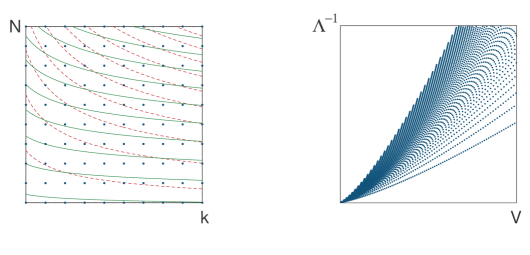
Figure 1: Left: Lattice of vacua in $(k,N)$-space. The green solid lines have constant $V$ and the red dashed lines constant $\Lambda^{-1}$. Both are increasing with $N$ and $k$. Right: Vacua mapped to $(V,\Lambda^{-1})$-space with $V\leq 200,\Lambda^{-1}\leq 2000$. The lower and upper boundaries correspond to $k=1$ resp. $N=1$.

For such a set of vacua labeled by $(N,k)$ we have (from the formulas in section 2.1.1)

$$kN^{3}=\Lambda^{-2}$$ (2.10)

$$kN^{7}=V^{6}.$$ (2.11)

We may now ask what the number of vacua is in a given region of $(V,\Lambda)$-space. This amounts to counting lattice points in the corresponding region in $(k,N)$-space, as illustrated in fig. 1. For sufficiently large regions, an estimate of this number is given by the area in $(k,N)$-space. Such an estimate is in general better for higher dimensional lattices and convex regions, but gives a reasonable approximation in this two-dimensional case as well, at least for sufficiently large regions, as we will demonstrate below.

Instead of computing the area in $(k,N)$ space, one can integrate a suitable vacuum number density over the region in $(V,\Lambda)$-space. This density is given by

$$d{\cal N} = dk\,dN\,\Theta(k-1)\,\Theta(N-1)$$ (2.12)

$$= d(V^{-9/2}\Lambda^{-7/2})\,d(V^{3/2}\Lambda^{1/2})\,\Theta(V^{-9/2}\Lambda^{-7/2}-1)\,\Theta(V^{3/2}\Lambda^{1/2}-1)$$

$$= \frac{3}{V^{4}\Lambda^{4}}\,dV\,d\Lambda\,\Theta(1-V^{9}\Lambda^{7})\,\Theta(V^{3}\Lambda-1)$$

$$= \frac{3(\Lambda^{-1})^{2}}{V^{4}}\,dV\,d\Lambda^{-1}\,\Theta(\Lambda^{-1}-V^{9/7})\,\Theta(V^{3}-\Lambda^{-1})$$ (2.13)

Here $\Theta(x)$ denotes the step function, equal to $1$ if $x\geq 0$ and $0$ otherwise. The last line is included for comparison with the discrete density in the $(V,\Lambda^{-1})$-plane shown in the figure.

We see for example that at fixed $\Lambda$, the density of vacua $d{\cal N}\sim dV/V^{4}$ is higher towards smaller volumes. However, this does not mean that in total there are more vacua at smaller volumes, as the step functions cut out an allowed region for $\Lambda$ that grows when $V$ increases. Going back to the original parametrization in terms of $k$ and $N$ (which is more useful to compare to the exact discrete distribution), we get that in the continuum approximation, the total number of vacua with bounded volume is given by

$${\cal N}_{\rm vac}(V_{X}\leq V_{*})=\int_{1}^{\infty}dN\int_{1}^{\infty}dk\,\Theta({V_{*}^{6}\over N^{7}}-k)$$ (2.14)

where the step function enforces the condition that we count $N$’s and $k$’s such that the volume is bounded by $V_{*}$ (i.e. the area under a solid green line in fig. 1). This integral gives the answer

$${\cal N}_{\rm vac}(V_{X}\leq V_{*})={V_{*}^{6}\over 6}+1-{7V_{*}^{6/7}\over 6}\sim V_{*}^{6}.$$ (2.15)

The subleading terms can be dropped since the continuum approximation requires $V_{*}\gg 1$. The leading term here arises from the small $N$ region so most of the vacua are here, as can be seen in the figure as well. So we find that the total number of vacua actually grows with the volume, in contrast to the decreasing $dV/V^{4}$ density at fixed $\Lambda$. Note that this $V_{*}^{6}$ growth is also quite different from the number of vacua with $V_{X}\leq V_{*}$ at fixed $k$, given by (2.8), which scales as $V_{*}^{6/7}$. Therefore, sampling topologies of the extra dimensions significantly changes the distribution of vacua.

These observations illustrate the obvious but important fact that the distribution of a quantity can depend strongly on the constraints and ensembles considered.

Another important issue is the validity of the continuum approximation. Thanks to the simplicity of this ensemble, we can compare our result (2.15) with the exact answer:

$$N_{\rm vac}(V_{X}\leq V_{*})=\sum_{k,N\geq 1}\Theta({V_{*}^{6}\over N^{7}}-k)\approx\sum_{1\leq N\leq V_{*}^{6/7}}\frac{V_{*}^{6}}{N^{7}}.$$ (2.16)

The approximation we made here (neglecting integrality of $k_{\rm max}$) becomes asymptotically exact in the large $V_{*}$ limit. In the same limit, the sum over $N$ gives a factor $\zeta(7)$, so

$$N_{\rm vac}(V_{X}\leq V_{*})\approx\zeta(7)V_{*}^{6}.$$ (2.17)

Since $\zeta(7)\approx 1.008$, this is about a factor 6 larger than the continuum result (2.15). The reason for this discrepancy is the fact that the region under consideration in the $(k,N)$-plane is very elongated along the $k$-direction, and most contributing lattice points are at the boundary $N=1$ (see fig. 1), so the integral is not a very accurate approximation of the sum. The continuum approximation will be better for regions in $(V,\Lambda)$-space that stay away from the boundary. Even in the case at hand though, the power of $V_{*}$ itself is correct, and since the coefficient is irrelevant at the level of accuracy we are working at anyway, the continuum approximation is satisfactory for our purposes.

Similarly we could ask how many vacua are there with $\Lambda\geq\Lambda_{*}$ (the other way around obviously gives a divergent answer). This is

$${\cal N}_{\rm vac}(\Lambda\geq\Lambda_{*})=\int_{1}^{\infty}dN\int_{1}^{\infty}dk\,\Theta({1\over\Lambda_{*}^{2}N^{3}}-k)\sim\Lambda_{*}^{-2}$$ (2.18)

Again this is a stronger growth than the fixed $k$ distribution (2.9).

¿From the joint distribution (2.12), one gets the distribution of one variable given the other one. As noted before, at fixed $\Lambda$, vacua accumulate towards the lower bound on the volume $V$, which is opposite to what one has for the distribution without constraint on $\Lambda$. For instance, when $\Lambda_{*}^{-2}\leq V_{*}^{6}$ and $\Lambda_{*}^{-2/3}\geq V_{*}^{6/7}$, one finds that ${\cal N}_{vac}(V\geq V_{*};\Lambda\geq\Lambda_{*})\sim\Lambda_{*}^{-3}V_{*}^{-3}$ which favors both small volume and cosmological constant.

In summary: we have shown that sampling the topology of the extra dimensions drastically changes the distribution of cosmological constants and volumes (i.e. eleven dimensional Planck scales). A priori, Freund-Rubin vacua statistically congregate in large volume, small cosmological constant regions. However, we saw that strong correlations between cosmological constant and volume exist, causing the effective distribution of one quantity to depend significantly on the constraints imposed on the other. For example at fixed cosmological constant, vacua actually prefer the lower volumes within the allowed range. Finally, we stressed that there exist at least as many non-supersymmetric, meta-stable Freund-Rubin vacua than supersymmetric.

One important point to keep in mind is that we have sampled a very simple set of Einstein manifolds. One would certainly like to know how representative the distribution of volumes and vacuum energies for the $(N,k)$ ensembles we studied is in the ensemble of all Einstein manifolds with positive scalar curvature. Some more complicated ensembles of Einstein 7-manifolds are described in [58, 59] and [58] gives a formula for the volumes which could be used to study the distributions of vacua as we have done here.

3 $\mathbf{G_{2}}$ Holonomy Statistics I: general results

$G_{2}$-holonomy vacua are compactifications of $M$ theory to four dimensions which, in the absence of flux classically give 4d ${\cal N}=1$ vacua with zero cosmological constant. These classical vacua have $b_{3}(X)$ complex moduli, of which the real parts are axions $t_{i}$ and the other half $s_{i}$ are the massless fluctuations of the metric on $X$.

The addition of fluxes when $X$ is smooth does not stabilise these moduli, as the induced potential is positive definite and runs down to zero at infinite volume. However, if $X$ has an orbifold singularity along a 3-manifold $Q$, additional non-Abelian degrees of freedom arise from massless membranes [57]. Nonabelian flux for these degrees of freedom then gives an additional contribution to the potential which can stabilise all the moduli if $Q$ admits a complex, non-real Chern-Simons invariant [3]. This is the case if, for instance, $Q$ is a hyperbolic manifold.

The vacua studied in [3] were supersymmetric with negative cosmological constant. In fact, it was shown that in the large radius approximation, for a given flux within a certain range, there is a single supersymmetric vacuum (in addition to an unstable de Sitter vacuum). In principle however there could be other, non-supersymmetric, vacua and one of our aims here is to study this possibility. One might wonder if any of these vacua could be metastable de Sitter. We will answer this question to a certain extent.

One of the difficulties in studying $G_{2}$-holonomy compactifications is that $G_{2}$-holonomy manifolds are technically very difficult to produce. For instance, we still do not know whether or not there exists a $G_{2}$-holonomy manifold with a non-real Chern-Simons invariant. So how can we hope to study the statistics of such vacua? As we will see below the superpotential of these $G_{2}$-compactifications with flux is very simple and does not contain much information about $X$. Instead, this information comes through the Kähler potential on moduli space, which could be a quite complicated function in general, of which very little is concretely known. One approach then is to try to obtain general results for an arbitrary Kähler potential. We will do this in the next section by extending some of the general techniques which were developed in the context mainly of IIB flux vacua in [6, 9, 20]. Secondly we could study particular ensembles of model Kähler potentials and hope that the results are representative in general. We will follow this approach in section 4, where we study a particular class of model Kähler potentials which allow explicit construction of all supersymmetric and nonsupersymmetric vacua.

3.1 $\mathbf{G_{2}}$ compactifications with fluxes and Chern-Simons invariants

Let $X$ be the $G_{2}$ holonomy compactification manifold. The complexified moduli space ${\cal M}$ of $X$ has dimension $n=b^{3}(X)$ and has holomorphic coordinates $z^{i}$, defined by

$$z^{i}=t^{i}+is^{i}=\frac{1}{\ell_{M}^{3}}\int C+i\varphi,$$ (3.1)

where $\varphi$ is the $G_{2}$-invariant 3-form on $X$ and $\ell_{M}$ is given by ${1/2\kappa_{11}^{2}}={2\pi/\ell_{M}^{9}}$. The metric on ${\cal M}$ is Kähler, derived from the Kähler potential [54]

$$K(z,\bar{z})=-3\ln\left(4\pi^{1/3}V_{X}(s)\right),$$ (3.2)

where $V_{X}\equiv\mbox{Vol}(X)/\ell_{M}^{7}$ is a homogeneous function of the $s^{i}$ of degree $7/3$. This classical metric will receive quantum corrections, but at large enough volumes such corrections can be argued to be small.

We turn on 4-form flux

$$G/\ell_{M}^{3}=N_{i}\rho^{i},$$ (3.3)

where $N_{i}\in\mathbb{Z}$ and $\rho^{i}$ is a basis of $H^{4}(X,\mathbb{Z})$, and also assume the presence of a complex Chern-Simons contribution as described above. This induces a superpotential [55, 56, 54, 3]

$$W(z)={1\over\kappa_{4}^{3}}(N_{i}z^{i}+c_{1}+ic_{2})$$ (3.4)

on ${\cal M}$, where $c_{1}$ and $c_{2}$ are the real and imaginary parts of the Chern-Simons invariant.

The corresponding potential is obtained from the standard four dimensional supergravity expression (for dimensionless scalars):

$$V=\kappa_{4}^{2}e^{K}\left(g^{i\bar{j}}F_{i}\bar{F}_{\bar{j}}-3|W|^{2}\right),$$ (3.5)

where

$$F_{i}\equiv D_{z^{i}}W\equiv(\partial_{z^{i}}+\partial_{z^{i}}K)W=N_{i}+\frac{1}{2i}\partial_{s^{i}}K\,W.$$ (3.6)

We will put $\kappa_{4}=1$ in what follows.

Since we are working in the large radius regime, the axions $t^{i}$ essentially decouple from the moduli $s^{i}$, and all nontrivial structure resides in the latter sector. This is seen as follows. Writing

$$W\equiv W_{1}(t)+i\,W_{2}(s),\qquad K_{i}\equiv\partial_{s^{i}}K(s),\qquad K_{ij}\equiv\partial_{s^{i}}\partial_{s^{j}}K=4g_{i\bar{j}}$$ (3.7)

and so on, the potential (3.5) becomes

$$V = e^{K}\left(4K^{ij}(\mbox{Re }F_{i})(\mbox{Re }F_{j})+K^{ij}K_{i}K_{j}W_{1}^{2}-3W_{1}^{2}-3W_{2}^{2}\right)$$ (3.8)

$$= e^{K}\left(4K^{ij}(\mbox{Re }F_{i})(\mbox{Re }F_{j})-3W_{2}(s)^{2}+4W_{1}(t)^{2}\right).$$

In the last line we used the fact that the volume $V_{X}$ is homogeneous of degree 7/3, which implies the following identities:

$$K_{i}s^{i}=-7,\qquad K_{ij}s^{j}=-K_{i}.$$ (3.9)

The second is obtained from the first by differentiation.

Since $W_{1}=N_{i}t^{i}+c_{1}$ and everything else in (3.8) depends only on $s$, it is clear that any critical point of $V$ will fix

$$N^{i}t_{i}+c_{1}=0$$ (3.10)

and therefore $W_{1}=\mbox{Im }F=0$. Apart from this, the $t^{i}$ are left undetermined, and they decouple from the $s^{i}$. From now on we will work on this slice of moduli space, so we can write

$$V=e^{K}\left(4K^{ij}F_{i}F_{j}-3W_{2}^{2}\right)$$ (3.11)

with

$$F_{i}=D_{s^{i}}W_{2}\equiv(\partial_{s^{i}}+\frac{1}{2}K_{i})W_{2}=N_{i}+\frac{1}{2}K_{i}(N_{j}s^{j}+c_{2}).$$ (3.12)

The geometry of the real moduli space ${\cal M}$ parametrized by the $s^{i}$ is the real analog of Kähler, often called Hessian, with metric $K_{ij}$.

3.2 Distribution of supersymmetric vacua over moduli space

The aim of this section is to find the distribution of vacua over ${\cal M}$, along the lines of [6, 9, 20]. The condition for a supersymmetric vacuum in the above notations is

$$D_{s^{i}}W_{2}(s)=0$$ (3.13)

In what follows we will drop the index $2$ to avoid cluttering. The number of solutions in a region ${\cal R}$ of ${\cal M}$, for all possible fluxes $G$ but at fixed $c_{2}$, is given by

$$N_{\rm susy}(c_{2},{\cal R})=\sum_{N\in\mathbb{Z}^{n}}\int_{{\cal R}}d^{n}s\,\delta^{n}(D_{i}W)|\det\partial_{i}D_{j}W|.$$ (3.14)

The determinant factor ensures every zero of the delta-function argument is counted with weight 1. An approximate expression ${\cal N}_{\rm susy}$ for the exact number of vacua $N_{\rm susy}$ is obtained by replacing the discrete sum over $N$ by a continuous integral, which is a good approximation if the number of contributing lattice points is large (which will be the case for sufficiently large $c_{2}$). Thus

$${\cal N}_{\rm susy}=\int_{{\cal R}}d^{n}s\int d^{n}N\,\delta^{n}(D_{i}W)|\det\partial_{i}D_{j}W|.$$ (3.15)

Differentiating (3.12) and using (3.13) and (3.9), one gets

$$\partial_{i}D_{j}W=\biggl{(}\frac{1}{2}K_{ij}-\frac{1}{4}K_{i}K_{j}\biggr{)}W=\frac{1}{2}K_{ik}\biggl{(}\delta^{k}_{j}+\frac{1}{2}s^{k}K_{j}\biggr{)}W$$ (3.16)

One eigenvector of the matrix in brackets is $s^{j}$, with eigenvalue $-5/2$ (this follows again from (3.9)). On the orthogonal complement $\{v|K_{j}v^{j}=0\}$, the matrix is just the identity, so all other eigenvalues are $1$. Thus,

$$|\det\partial_{i}D_{j}W|=\frac{5|W|^{n}}{2^{n+1}}\det K_{ij}$$ (3.17)

Furthermore, by contracting (3.12) with $s^{i}$, we get at $F_{i}=0$:

$$W=-\frac{2}{5}c_{2}.$$ (3.18)

To compute (3.15), we change variables from $N_{i}$ to $F_{i}$. The Jacobian is

$${\rm Jac}=|\det\partial_{N_{i}}F_{j}|^{-1}=|\det(\delta^{i}_{j}+\frac{1}{2}K_{j}s^{i})|^{-1}=2/5.$$ (3.19)

Putting everything together, we get

$${\cal N}_{\rm susy} = \int_{{\cal R}}d^{n}s\int d^{n}F\,\delta^{n}(F)\,\biggl{(}\frac{c_{2}}{5}\biggr{)}^{n}\det K_{ij}$$ (3.20)

$$= \biggl{(}\frac{c_{2}}{5}\biggr{)}^{n}\int_{{\cal R}}d^{n}s\det K$$ (3.21)

$$= \biggl{(}\frac{4c_{2}}{5}\biggr{)}^{n}\mbox{Vol}(\widehat{{\cal R}})$$ (3.22)

where $\widehat{{\cal R}}$ is the part of the complexified moduli space projecting onto ${\cal R}$ (i.e. the direct product of ${\cal R}$ with the $n$-torus $[0,1]^{n}$ swept out by the axions $t^{i}$), and the volume is measured using the Kähler metric $g_{i\bar{j}}=K_{ij}/4$ on this space.

Thus, supersymmetric vacua are distributed uniformly over moduli space. This result is similar to the Type IIB orientifold case studied in [9], but simpler: the Type IIB vacuum number density involves curvature terms as well, and in order to get a closed form expression for $n>1$, it was necessary there to count vacua with signs rather than their absolute number.

Note that in any finite region of moduli space, the number of vacua is finite, because $c_{2}$ is finite despite the absence of a tadpole cutoff on the fluxes. In particular, the total number of vacua in the large radius region of moduli space (where our computation is valid) is finite. For IIB vacua on the other hand, finiteness is only obtained after imposing the tadpole cutoff $\int F\wedge H\leq L_{*}=\chi/24$ on the fluxes. In a way, the Chern-Simons invariant $c_{2}$ plays the role of $L_{*}$ here.

Example

The simplest example is the case $n=1$. Then homogeneity fixes $V_{X}\sim s^{7/3}$, so $K_{ss}=\frac{7}{s^{2}}$, and

$${\cal N}_{\rm susy}(c_{2},s\geq s_{*})=\frac{c_{2}}{5}\int_{s_{*}}^{\infty}ds\,\frac{7}{s^{2}}=\frac{7}{5}\frac{c_{2}}{s_{*}}.$$ (3.23)

Thus, vacua become denser towards smaller volume of $X$, and from this equation one would estimate there are no vacua with $s>7c_{2}/5$, which is where ${\cal N}_{\rm susy}$ drops below 1. Indeed, it is easily verified that the exact critical point solution is $s=-7c_{2}/5N$, so the largest possible value of $s$, obtained at $N=-1$, is precisely $7c_{2}/5$. Better even, from the explicit solution it easily follows that the approximate distribution (3.23) becomes in fact exact by rounding off the right hand side to the nearest smaller integer.

3.3 Large volume suppression

Although the precise form of the metric for $n>1$ is unfortunately not known, one general feature is easy to deduce: flux vacua with large compactification volume are suppressed, and strongly so if the number of moduli is large. This follows from simple scaling. If $s\to\lambda s$, $K$ shifts with a constant, so $K_{ij}\to\lambda^{-2}K_{ij}$ and the measure $d^{n}s\det K\to\lambda^{-n}\,d^{n}s\det K$. Thus we have for example

$${\cal N}_{\rm susy}(c_{2},s^{i}\geq s_{*})=(c_{2}/s_{*})^{n}\,{\cal N}_{\rm susy}(1,s^{i}\geq 1),$$ (3.24)

and

$${\cal N}_{\rm susy}(c_{2},V_{X}\geq V_{*})=k_{n}\left(c_{2}/V_{*}^{3/7}\right)^{n},$$ (3.25)

where $k_{n}$ is independent of $c_{2}$ and $V_{*}$. Hence large compactification volume is strongly suppressed when $n$ is large.

To get an estimate for the absolute number of vacua with $V_{X}\geq V_{*}$, one would need to estimate $k_{n}$ in (3.25). This would be quite hard in general even if the metric was explicitly known, so to get an idea let us do this for a simple toy model, taking the volume to be the following homogeneous function of degree $7/3$:

$$V_{X}(s)=\biggl{(}\sum_{i}s_{i}^{2}\biggr{)}^{7/6}.$$ (3.26)

Then $K=-\frac{7}{2}\log(s^{2})$,

$$K_{ij}=\frac{7}{s^{2}}\biggl{(}2\frac{s_{i}s_{j}}{s^{2}}-\delta_{ij}\biggr{)},$$ (3.27)

and

$$|\det K|=\biggl{(}\frac{7}{s^{2}}\biggr{)}^{n}.$$ (3.28)

This metric is actually not positive definite for $n>1$ and therefore unphysical, but let us proceed anyway. A more sensible model will be presented in the next section. We have $V_{X}\geq V_{*}$ iff $|s|\geq s_{*}$, with $s_{*}\equiv V_{*}^{3/7}$. Thus

$${\cal N}_{\rm susy}(c_{2},V_{X}\geq V_{*}) = \biggl{(}\frac{7c_{2}}{5}\biggr{)}^{n}\int_{|s|\geq s_{*}}d^{n}s\,\frac{1}{s^{2n}}$$ (3.29)

$$= \biggl{(}\frac{7c_{2}}{5}\biggr{)}^{n}\Omega_{n-1}\frac{1}{ns_{*}^{n}},$$ (3.30)

where $\Omega_{n-1}=\frac{2\pi^{n/2}}{\Gamma(n/2)}$ is the area of the $(n-1)$-dimensional sphere of radius 1. So

$${\cal N}_{\rm susy}(c_{2},V_{X}\geq V_{*}) = \biggl{(}\frac{7c_{2}}{5}\biggr{)}^{n}\frac{\pi^{n/2}}{(n/2)!}\frac{1}{s_{*}^{n}}$$ (3.31)

$$\approx \biggl{(}\frac{7\sqrt{2\pi e}}{5}\frac{c_{2}}{s_{*}\sqrt{n}}\biggr{)}^{n}\approx\biggl{(}\frac{6\,c_{2}}{\sqrt{n}s_{*}}\biggr{)}^{n}.$$ (3.32)

In going from the first to the second line we used Stirling’s approximation $m!\approx(m/e)^{m}$, valid for large $m$.

This confirms the general result based on scaling, but now we also have information about the absolute numbers. In particular, this formula suggests all vacua for this toy model must have compactification volume approximately bounded by

$$V_{X}<\biggl{(}\frac{6\,c_{2}}{\sqrt{n}}\biggr{)}^{7/3}.$$ (3.33)

Similar bounds can be expected for other models, as we confirm in section 4. In general, large extra dimension scenarios with, say, micrometer scale compactification radii are therefore excluded in these ensembles unless $c_{2}$ is exceedingly large.

3.4 Distribution of supersymmetric cosmological constants

The vacuum energy in a supersymmetric vacuum is, in 4d Planck units, using (3.18):

$$\Lambda=-3e^{K}|W|^{2}=-\alpha{c_{2}^{2}\over V_{X}^{3}}$$ (3.34)

where $\alpha=3/400\,\pi\approx 0.002$. Therefore, the only way to get a small cosmological constant is to have large compactification volume. This contrasts with the ensemble of type IIB flux vacua, where very small cosmological constants can be obtained at arbitrary complex structure (i.e. arbitrary mirror IIA volume). The underlying reason is the fact that in IIB, there are four times as many fluxes as equations $D_{i}W=0$, so at a given point, there is still a whole space of (real) fluxes solving the equations. This freedom can be used to tune the cosmological constant to a small value. Here on the other hand, there is only one flux per equation, so at a given $s$, the fluxes are completely fixed, and no freedom remains to tune the cosmological constant. This would likely change however if more discrete data were turned on, such as the $M$ theory duals of IIA RR 2-form flux or IIB NS 3-form flux. Unfortunately these are difficult to describe systematically in $M$ theory in a way suitable for statistical analysis.

Let us compute the distribution of cosmological constants more precisely. Equation (3.34) implies that this follows directly from the distribution of volumes. Using (3.25), we get

$${\cal N}_{\rm susy}(c_{2},|\Lambda|\leq\lambda_{*})=k_{n}\biggl{(}{c_{2}^{5}\lambda_{*}\over\alpha}\biggr{)}^{n/7}.$$ (3.35)

The corresponding distribution density is therefore

$$d{\cal N}/d\lambda\sim\lambda^{(n-7)/7}.$$ (3.36)

In particular, for $n<7$, the distribution diverges at $\lambda=0$, while for $n>7$, the density goes to zero. In the toy model, from (3.33), we get an expected bound:

$$|\Lambda|>{\alpha\,n^{7/2}\over 6^{7}c_{2}^{5}}.$$ (3.37)

For large $n$, this is much larger than the naive $1/{\cal N}_{\rm susy}$ which was found to be a good estimate in the Type IIB case, where the cosmological constants of supersymmetric vacua are always distributed uniformly near zero [9].

Because $G_{2}$ manifolds with many moduli are much more numerous than those with only a few, we can thus conclude that small cosmological constants are (without further constraints) strongly suppressed in the ensemble of all supersymmetric $G_{2}$ flux vacua.

3.5 Nonsupersymmetric vacua

A vacuum satisfies $V^{\prime}=0$, and metastability requires $V^{\prime\prime}>0$. Thus, the number of all metastable vacua in a region ${\cal R}$ is given by

$$N_{vac}=\sum_{N}\int_{{\cal R}}d^{n}s\,\delta(V^{\prime})\,|\det V^{\prime\prime}|\,\Theta(V^{\prime\prime}).$$ (3.38)

In principle one could again approximate the sum over $N$ by an integral and try to solve the integral by changing to appropriate variables, as we did for the supersymmetric case in section 3, and as was done in [20] for supersymmetry breaking scales well below the fundamental scale. In practice, we will encounter some difficulties doing this for $G_{2}$ vacua.

By differentiating equation (3.11), one gets

$$\partial_{i}V=e^{K}(8(D_{i}D_{j}W)D^{j}W-6\,WD_{i}W)$$ (3.39)

where $D_{i}$ denotes the Hessian Levi-Civita plus Kähler covariant derivative. The matrix $M_{ij}\equiv D_{i}D_{j}W$ is related to the fermionic mass matrix, and with this notation the critical point condition becomes

$$M_{ij}F^{j}=\frac{3}{4}WF_{i}.$$ (3.40)

In [20], a similar equation was interpreted at a given point in moduli space as a linear eigenvalue equation for the supersymmetry breaking parameters $F$, assuming the matrix $M$ (denoted $Z$ there) to be independent of $F$. This is indeed the case for the Type IIB flux ensemble, but it is not true for the $G_{2}$ ensemble. The reason is again the fact that there are only as many fluxes as moduli here, so a complete set of variables parametrizing the fluxes $N_{i}$ is already given by the $F_{i}$ (affinely related to the $N_{i}$ as expressed in (3.12)). Therefore, all other quantities such as $W$ and $M_{ij}$ and so on must be determined by the $F_{i}$. Indeed, a short computation gives:

$$W = -\frac{2}{5}(s^{i}F_{i}+c_{2})$$ (3.41)

$$M_{ij} = \frac{1}{2}\bigl{(}(K_{ij}-\frac{1}{2}K_{i}K_{j})W+K_{i}F_{j}+K_{j}F_{i}-K^{k}_{ij}F_{k}\bigr{)}$$ (3.42)

This means that at a given point in moduli space, (3.40) is actually a complicated system of quadratic equations in $F$, with in general only one obvious solution, the supersymmetric one, $F=0$. In total one can expect up to $2^{n}$ solutions for $F$. The nonsupersymmetric solutions will generically be of order $c_{2}$. In particular it is not possible to tune fluxes to make $F$ parametrically small, so it is not possible to use the analysis of [20] here, and there is no obvious perturbation scheme to compute (3.38).

Example

As a simple example we take the case $n=1$. As noted in section 3.2, homogeneity then forces $K=-7\ln s$, hence $M_{ss}=(7c_{2}-5Fs)/2s^{2}$, and (3.40) (considered as an equation for $F$ at fixed $s$) has solutions $F=0$ and $F=\frac{14\,c_{2}}{s}$. Neglecting the metastability condition, the continuum approximated number density of nonsupersymmetric vacua is given by

$$d{\cal N}_{\rm nonsusy} = \int dN\,\delta(F-\frac{14\,c_{2}}{s})\,|\partial_{s}(F-\frac{14\,c_{2}}{s})|\,ds$$ (3.43)

$$= \int\frac{2}{5}\,dF\,\delta(F-\frac{14\,c_{2}}{s})\,\frac{35\,c_{2}}{2\,s^{2}}\,ds$$

$$= \frac{7\,c_{2}}{s^{2}}\,ds.$$

We changed variables from $N$ to $F$ in the integral using the Jacobian (3.19). This result should be compared to the supersymmetric density implied by (3.23):

$$d{\cal N}_{\rm nonsusy}=5\,d{\cal N}_{\rm susy}.$$ (3.44)

This does not mean that for a given flux, there are on average five nonsupersymmetric critical points for every supersymmetric one. In fact, as we will see below, and as was already pointed out in [3], for $n=1$, there is exactly one nonsupersymmetric critical point for every supersymmetric one: the supersymmetric minimum is separated from $s=\infty$ by a barrier, whose maximum is the (de Sitter, unstable) nonupersymmetric critical point. Equation (3.44) only expresses that in a given region of moduli space (at large $s^{i}$), there are on average 5 times more nonsupersymmetric vacua then supersymmetric ones. This is simply because in the region of moduli space under consideration, the nonsupersymmetric critical points are located at five times the value of $s$ of the supersymmetric critical points.

3.6 Supersymmetry breaking scales

For more moduli, things become more complicated. A few useful general observations can be made though. If we require $V=0$ (which remains a good approximation for what follows as long as $|V|\ll e^{K}c_{2}^{2}$) we can make a fairly strong statement about the value of the supersymmetry breaking scale. Contracting (3.40) with $s^{i}$ and using (3.41)-(3.42) and (3.9), we get

$$25\,F^{2}-3(s\cdot F)^{2}-8\,c_{2}(s\cdot F)=0.$$ (3.45)

Together with $V\sim 4F^{2}-3W^{2}=0$, this gives a system of two equations in two variables, $s\cdot F$ and $F^{2}$, with solutions:

$$F^{2}=\frac{3c_{2}^{2}}{4},\qquad s\cdot F=\frac{3c_{2}}{2}.$$ (3.46)

The physical supersymmetry breaking scale for such vacua (assuming they exist) is

$$M_{\rm susy}^{2}\equiv m_{p}^{2}\sqrt{4e^{K}K^{ij}F_{i}F_{j}}=\frac{\sqrt{3}\,c_{2}\,m_{p}^{2}}{8\sqrt{\pi}\,V_{X}^{3/2}}\sim\frac{M_{p}^{3}c_{2}}{m_{p}},$$ (3.47)

where $m_{p}\equiv 1/\kappa_{4}$ and $M_{p}$ are the 4- and 11-dimensional Planck scales.

Let us plug in some numbers to get an idea of the implications. If we identify $M_{p}$ with the unification scale $M_{\rm unif}\sim 10^{16}\,{\rm Gev}$, this means that $M_{\rm susy}\sim\sqrt{c_{2}}\,10^{14.5}\,{\rm GeV}$, and the gravitino mass $M_{g}\sim M_{\rm susy}^{2}/m_{p}\sim c_{2}\,10^{10}\,{\rm GeV}$. Since $c_{2}$ is at least of order 1, this estimate implies (under the given assumptions) that in this ensemble supersymmetry is always broken at a scale much higher than what would be required to get the electroweak scale $M_{\rm ew}\sim 100\,{\rm GeV}$ without fine tuning.

In fact a slight extension of this calculation shows that even if one allows the addition of an arbitrary constant to the potential to reach $V=0$ (e.g. to model D-terms or contributions from loop corrections), the supersymmetry breaking scale in this ensemble is still bounded from below by the scale $c_{2}M_{p}^{3}/m_{p}$.

One could of course question the identification $M_{p}\sim M_{\rm unif}$. Lowering the 11d Planck scale down to $M_{p}\sim 10^{13}\,{\rm Gev}$ for example (which requires $V_{X}\sim 10^{12}$) gives a supersymmetry breaking scale $M_{\rm susy}\sim\sqrt{c_{2}}\,10^{10}\,{\rm Gev}$ and gravitino mass $m_{g}\sim c_{2}\,10\,{\rm Gev}$, which for $c_{2}$ not too large would give low energy supersymmetry.

Note however that in analogy with the supersymmetric case, and based on general considerations, we expect suppression of vacua at large volume and therefore also suppression of low energy supersymmetry breaking scales in this ensemble. This is further confirmed by the exactly solvable models we will present in section 4. In particular we get a lower bound on the supersymmetry breaking scale from the upper bound on the volume $V_{X}$, which in general we expect to be of the form (3.33), i.e. $V_{X}<(c_{2}/r_{n})^{7/3}$, with $r_{n}$ weakly growing with $n$. Using the relation (3.47) between $M_{\rm susy}$ and $V_{X}$, this implies the following lower bound for the supersymmetry breaking scale

$$M_{\rm susy}/m_{p}>\frac{r_{n}^{7/4}}{c_{2}^{5/4}}.$$ (3.48)

Getting $M_{\rm susy}$ below $10^{12}\,{\rm Gev}$ in the case of many moduli would thus require $c_{2}$ to be at least of order $10^{6}$.

Using the volume distribution (3.25), we furthermore get an estimate for the distribution of supersymmetry breaking scales (in 4d Planck units):

$$d{\cal N}_{\rm nonsusy}\sim\tilde{k}_{n}\,c_{2}^{5n/7}d(M_{\rm susy}^{4n/7})/m_{p}^{4n/7},$$ (3.49)

where $\tilde{k}_{n}$ is a constant independent of $c_{2}$ and $M_{*}$.

Here we have not yet taken into account the tuning required to get a tiny cosmological constant: $|\Lambda|\sim|4F^{2}-3W^{2}|/V_{X}^{3}<\Lambda_{*}$. For a given volume $V_{X}$ (or equivalently a given supersymmetry breaking scale), this requires tuning the fluxes such that $|4F^{2}-3W^{2}|<\Lambda_{*}V_{X}^{3}$, which can be expected to at least add another suppression factor $\Lambda_{*}V_{X}^{3}\sim\Lambda_{*}/M_{\rm susy}^{4}$. The suppression may in fact be stronger, if the distribution of cosmological constants is not uniform but more like a Gaussian sharply peaked away from $\Lambda=0$. Such distributions are quite plausible in these ensembles, as will be illustrated by the model ensemble we will study in section 4. Another potentially important factor which we are neglecting in this analysis is the metastability constraint (this was found in [20] to add another factor $M_{\rm susy}^{4}$ to the distribution in the ensembles studied there).

Finally, when one also takes into account the observed value of the electroweak scale $M_{\rm ew}$, there is an additional expected tuning factor presumably of order $M_{\rm ew}^{2}m_{p}^{2}/M_{\rm susy}^{4}$ (in the region of parameter space where this is less than 1) [17, 18, 19]. Putting everything together, this gives (for $m_{p}^{2}>M_{\rm susy}^{2}>M_{\rm ew}m_{p}$):

$$d\,{\cal N}\sim\tilde{k}_{n}\,\Lambda_{*}\,M_{\rm ew}^{2}\,c_{2}^{5n/7}|d\,M_{\rm susy}^{4(n/7-2)}|/m_{p}^{4n/7-2}$$ (3.50)

So we see that for $n<14$, the Higgs mass and cosmological constant tunings tilt the balance to lower scales, while for $n>14$ higher scales are favored, and strongly so if $n$ is large. For $n<14$ we should keep in mind however that there is an absolute lower bound on the supersymmetry breaking scale, given by (3.48), which will further be increased by the additional tunings of cosmological constant and Higgs mass. We should also not forget that this is only a naive analysis; in principle a full computation of the measure should be done along the lines of [20], but as we discussed, this does not seem possible in the present context, because of the absence of a small parameter.

Nevertheless, the above consideration indicate clearly that low energy supersymmetry is typically disfavored in $G_{2}$ flux ensembles, and even excluded if $c_{2}$ is less than $10^{6}$.

4 $\mathbf{G_{2}}$ statistics II: model Kähler potentials and exact solutions

In the previous section we obtained a number of general results about distributions of $G_{2}$ flux vacua, independent of the actual form of the Kähler potential. For nonsupersymmetric vacua the results were less detailed, mainly because the constraint $V^{\prime}=0$ is quadratic in $F$, and, unlike the situation in [20], no regime exists in which the equations can be linearized. To make further progress, we will now study a class of model Kähler potentials for which all vacua can be computed explicitly.

In general, at large volume, the Kähler potential is given by (3.2): $K=-3\log(4\pi^{1/3}V_{X})$, where $V_{X}$ is the volume of $X$ regarded as a function of the moduli $s_{i}$. Unlike the case of a Calabi-Yau, where the volume function is always a third order homogeneous polynomial in the Kähler moduli, no strong constraints on $V_{X}$ are known for $G_{2}$ holonomy manifolds — just that the volume function is homogeneous of degree $7/3$ and that minus its logarithm is convex, i.e. the second derivative of $K$, which gives the kinetic energies of the moduli, is positive definite. In general it is difficult to find simple candidate volume functions which satisfy this positivity constraint. The most general homogeneous degree $7/3$ function is of the form

$$V_{X}=\prod_{k=1}^{n}s_{k}^{a_{k}}f(s_{i})$$ (4.1)

with $\{a_{k}\}$ such that

$$\sum_{k=1}^{n}a_{k}=\frac{7}{3}.$$ (4.2)

and $f(s_{i})$ invariant under scaling. If we now suppose that we are in a region of moduli space where $f(s_{i})$ is approximately constant then we can take

$$V_{X}=\prod_{k=1}^{n}s_{k}^{a_{k}},$$ (4.3)

and this in fact gives a positive moduli space metric. This justifies this particular choice of Kahler potentials.

The above choice of $V_{X}$ gives a simple geometry to the moduli space which is quite natural. The Kähler metric is

$$ds^{2}=\sum_{i=1}^{n}\frac{3a_{i}}{4s_{i}^{2}}dz_{i}d\bar{z}_{i}=\sum_{i=1}^{n}\frac{3a_{i}}{4s_{i}^{2}}(dt_{i}^{2}+ds_{i}^{2})$$ (4.4)

This is locally the metric of the product of $n$ hyperbolic planes $\mathbf{H}^{2}$, which is:

$$ds^{2}=\frac{1}{\l^{2}x^{2}}(dx^{2}+dy^{2})$$ (4.5)

where $\l$ is connected to the curvature tensor by

$$\hat{R}_{12}=-\l^{2}e_{1}\wedge e_{2}$$ (4.6)

So locally the moduli space is $\mathbf{H}^{2n}$. Globally it is given by $\mathbf{H}^{2n}/\mathbb{Z}^{n}$, because the axions $t_{i}$ are periodic variables. In this class of $n$-parameter Kähler potentials labeled by $a_{i}$, all the information about $X$ is contained in the values of the $a_{i}$. Since the moduli space metric (equivalently moduli kinetic terms) is singular if $a_{i}=0$ and the moduli have the wrong sign kinetic terms if $a_{i}<0$, we take $a_{i}>0$. We will not restrict to any other particular values for the $a_{i}$ if it is not necessary to do so.

The potential on the moduli space is given by (3.8):

$$V=\frac{c_{2}^{2}}{48\pi\,V_{X}^{3}}\biggl{(}3+\sum_{j=1}^{n}a_{j}\nu_{j}s_{j}(\nu_{j}s_{j}-3)\biggr{)}+\frac{1}{48\pi\,V_{X}^{3}}(\vec{N}\cdot\vec{t}+c_{1})^{2}.$$ (4.7)

where $\nu_{j}\equiv-\frac{N_{j}}{c_{2}a_{j}}$.

4.1 Description of the Vacua

We now describe the vacua ie the critical points of $V$. The equations for the axions give

$$\vec{N}\cdot\vec{t}+c_{1}=0$$ (4.8)

which fixes this particular linear combination of axions. We are not concerned with fixing the remaining axions, since they are compact fields and will be fixed by any non-perturbative corrections. Our interest is in the moduli $s_{i}$. The equations of motion for the $s_{i}$ reduces to a system of $n$ quadratic equations. For the case at hand these are equivalent to:

$$\sum_{j=1}^{n}3a_{j}h_{j}(h_{j}-3)-2h_{i}^{2}+3h_{i}+9=0,$$ (4.9)

where we defined $h_{j}\equiv\nu_{j}s_{j}$ (no sum). Note that this system separates in $n$ quadratic equations in one variable $h_{i}$. The solutions are therefore of the form

$$h_{i}=\frac{3}{4}+m_{i}H$$ (4.10)

where $m_{i}=+1$ or $-1$, and $H$ is determined by substituting this in (4.9). This results in a single quadratic equation:

$$5H^{2}-\frac{9}{2}AH-\frac{27}{16}=0.$$ (4.11)

where

$$A\equiv\vec{a}\cdot\vec{m}.$$ (4.12)

A priori therefore, $H$ can take two possible values:

$$H^{\pm}_{(\vec{m})}=\frac{3}{20}\left(3A\pm\sqrt{9A^{2}+15}\right)$$ (4.13)

However, because

$$H^{+}_{(\vec{m})}=-H^{-}_{(-\vec{m})}$$ (4.14)

we only ever need to consider, say, the negative branch of the square root to get all solutions in (4.10). In total, therefore, the number of vacua for a fixed choice of fluxes is $2^{n}$. We choose the following parametrisation: take all $2^{n}$ choices for $\vec{m}$. Then

$$h^{(\vec{m})}_{i}={3\over 4}+m_{i}H_{(\vec{m})}$$ (4.15)

with $H\equiv H^{-}$.

We can thus think of the vacua as the states of a system with $n$ “spins” $m_{i}$. When all spins are aligned with the “external field” $\vec{a}$, that is if all $m_{i}=+1$, we have

$$A=7/3,\quad h_{i}={3\over 5}$$ (4.16)

When all spins are anti-aligned ($m_{i}=-1$), this becomes

$$A=-7/3,\quad h_{i}=3.$$ (4.17)

The first of these can be shown to be the supersymmetric AdS vacuum discussed in [3] whilst the second is the unstable de Sitter vacuum also discussed there. The remaining $2^{n}-2$ are all non-supersymmetric and could be either de Sitter or anti de Sitter. The metastability of these vacua will be analyzed in section 4.2.

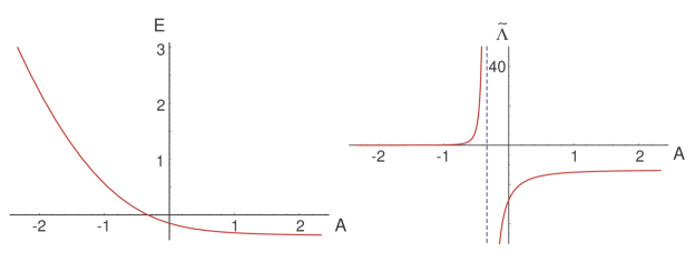
Figure 2: Left: $E$ as a function of $A\equiv\vec{a}\cdot\vec{m}$. Here $E(-7/3)=3$ and $E(7/3)=-9/25$. Right: dependence of $\tilde{\Lambda}$ on $A$. At $A=-7/3$, $\tilde{\Lambda}\approx 10^{-3}$, and at $A=7/3$, $\tilde{\Lambda}\approx-13$. The divergence at $A=-1/3$ is due to the vanishing of the volume there.

Substituting (4.15) in (4.7), we get that the energy of these vacua is given by $V=\frac{c_{2}^{2}}{48\pi V_{X}^{3}}E$ with $E=\frac{2}{3}H^{2}-\frac{3}{8}$. At fixed volume, the vacuum energy varies only through $E$. The dependence of $E$ on $A$ is shown on the left in fig. 2. However, the volume depends on $\vec{m}$ as well:

$$V_{X}=\prod_{i=1}^{n}s_{i}^{a_{i}}=\prod_{i=1}^{n}\left(\frac{c_{2}a_{i}}{|N_{i}|}\right)^{a_{i}}\prod_{i=1}^{n}|h_{i}|^{a_{i}},$$ (4.18)

so the total vacuum energy is, up to $\vec{m}$-independent factors:

$$\Lambda\sim\tilde{\Lambda}\equiv E\,\prod_{i=1}^{n}|h_{i}|^{-3a_{i}}=E\,\bigl{|}\frac{3}{4}+H\bigr{|}^{-\frac{7}{2}-\frac{3A}{2}}\,\bigl{|}\frac{3}{4}-H\bigr{|}^{-\frac{7}{2}+\frac{3A}{2}}.$$ (4.19)

The dependence of this on $A$ is shown on the right in fig. 2. The divergence at $A=-1/3$ is due to the vanishing of the volume there, as all $h_{i}$ with $m_{i}=+1$ vanish at this point. Obviously the supergravity approximation breaks down in this regime. One notable fact is further that the smallest positive cosmological constant is obtained when all spins are down, while the smallest negative cosmological constant (in absolute value) is obtained when all spins are up, i.e. at the supersymmetric critical point.

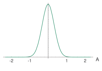
Figure 3: Distribution of $A$ values for $a_{i}=7n/3$, $n=50$.

At large $n$, the vast majority of vacua will be “halfway” the extrema. More precisely, if say all $a_{i}=a=7/3n$, the variable $A$ will be binomially distributed around $A=0$, as illustrated in 3. At large $n$ this distribution asymptotes to the continuous normal density

$$d{\cal N}[A]\approx\frac{2^{n}}{\sqrt{2\pi}\sigma}\exp\bigl{(}-\frac{A^{2}}{2\sigma^{2}}\bigr{)}\,dA;\qquad\sigma=\frac{7}{3\sqrt{n}}.$$ (4.20)

For large $n$ this is sharply peaked around $A=0$, for which $E=-3/20$ and $|F|^{2}=\frac{119}{80}c_{2}^{2}$, so the majority of vacua are AdS and break supersymmetry at a scale $M_{\rm susy}^{2}=|F|/V_{X}^{3/2}\sim c_{2}M_{p}^{3}/m_{p}$.

Thus far we have considered solutions in terms of $h_{i}$. The actual values of the moduli are given by

$$s_{i}=-\frac{c_{2}a_{i}h_{i}}{N_{i}}.$$ (4.21)

Since the moduli fields $s_{i}$ are positive in the supergravity approximation, the signs of the $h_{i}$ and flux quanta $N_{i}$ must be correlated. Without loss of generality we take $c_{2}$ to be positive. Then $N_{i}$ and $h_{i}$ must have opposite signs. Now as long as $A>-1/3$, every $h_{i}$ is automatically positive, so any such vacuum must have negative $N_{i}$. When $A<-1/3$, $h_{i}$ is positive if $m_{i}=-1$ and negative if $m_{i}=+1$, so these vacua must have $\mbox{sign }N_{i}=\mbox{sign }m_{i}$. Recall that the condition $A<-1/3$ is also the condition to have $E>0$.

Thus, for any given $\vec{m}$, there is a unique choice of sign for each $N_{i}$ which renders all $s^{j}$ positive for all choices of $|N_{i}|$.

On the other hand, not all given, fixed fluxes $N$ gives rise to the same number of vacua. The following cases can be distinguished:

• All $N_{i}<0$: set of vacua = $\{\vec{m}|A\equiv\vec{a}\cdot\vec{m}>-1/3\}\cup\{(-1,-1,\cdots,-1)\}$. All vacua in the first set are AdS. The additional one is dS (but is unstable, as we will discuss in the next section). There are of order $2^{n}$ such vacua (between $2^{n-1}$ and $2^{n}$ for example when all $a_{i}$ are equal as for the distribution of fig. 2).

• Some $N_{i}>0$, and $\vec{a}\cdot\mbox{sign}(\vec{N})<-1/3$: just one vacuum, given by $m_{i}=\mbox{sign}(N_{i})$. This vacuum is dS (but again will turn out to be unstable).

• Some $N_{i}>0$, and $\vec{a}\cdot\mbox{sign}(\vec{N})>-1/3$: no vacua.

As noted before, the choices of $\vec{m}$ for which $A$ is at or near $-1/3$ do not correspond to vacua within the region of validity of our computations for reasonable values of $c_{2}$, because some of the moduli, and hence the volume, will be at or near zero then.

4.2 Metastability

We now turn to the question of metastability. We found that all dS vacua (i.e. the vacua with $A<-1/3$) for our model ensembles have a tachyon and hence are perturbatively unstable. The proof can be found in appendix B. We therefore focus on AdS vacua in what follows.

In general the condition for the perturbative stability of an AdS vacuum is the Breitenlohner-Freedman bound [60], which is given by

$$\hat{\partial}_{i}\hat{\partial}_{j}V-\frac{3}{2}V\delta_{ij}\geq 0$$ (4.22)

where the derivatives are with respect to the canonically normalised scalars, or equivalently the Hessian is expressed in an orthonormal frame.

The details of the stability analysis are somewhat technical and are given in appendix B. We find that exponentially large numbers of the $2^{n}$ vacua are in fact metastable. Specifically, vacua for which $A>{1\over 3}$ are always metastable. Vacua with $-{1\over 3}<A<{1\over 3}$ can in principle also be metastable (and actually turn out to be local minima), but this is rather exceptional: they correspond to having only one of the $m_{i}$ equal to $+1$. In particular, since $\sum_{i}a_{i}=7/3$, this means that the corresponding $a_{i}$ must be greater than $1$, and thus there cannot be more than two such solutions.

Some lower bounds on the numbers of metastable vacua with $A\geq 1/3$ can be derived as follows. For simplicity, but without loss of generality, we put

$$a_{n}\geq a_{n-1}\geq\ldots\geq a_{1}.$$ (4.23)

When $a_{n}\geq\frac{4}{3}$, all solutions with $m_{n}=+1$ correspond to $A\geq\frac{1}{3}$, and we have

$$N_{\rm stab}\geq 2^{n-1}$$ (4.24)

one of which is the supersymmetric solution. When $a_{n}+a_{n-1}\geq\frac{4}{3}$ the number of stable vacua is at least

$$N_{\rm stab}\geq 2^{n-2}$$ (4.25)

and so on. So in a model with $a_{n}+a_{n-1}+\ldots+a_{n-j+1}\geq\frac{4}{3}$, but with $a_{n}+a_{n-1}+\ldots+a_{n-j}<\frac{4}{3}$, the number of stable vacua is at least

$$N_{\rm stab}\geq 2^{n-j}$$ (4.26)

Because of (4.23) and the fact that $\sum a_{i}={7\over 3}$, we cannot have $j>4n/7$. So for a model with $n$ moduli, the number of stable vacua is surely bigger than

$$N_{\rm stab}\geq 2^{n-4n/7}=2^{3n/7},$$ (4.27)

which is exponentially smaller than $2^{n}$ but still exponential in $n$.

Actually this number is very hard to reach and for generic models the number of stable vacua is much bigger than this. Take for example the case $a_{i}=3/7n$ of the figure, for which $\tilde{A}=\frac{3}{7}A$ is distributed according to (4.20) in the large $n$ limit. The number of vacua with $A>1/3$ is then given by integrating the distribution (4.20) from $A=1/3$ to $A=\infty$. At large $n$ this gives asymptotically

$$N_{\rm stab}/2^{n}\approx\frac{7}{\sqrt{2\pi n}}\exp(-n/98).$$ (4.28)

Again for large $n$ this is an exponentially small fraction, but still exponentially large in absolute number. In fact for $n=100$ the stable fraction is still about $10\%$. For $n=1000$, this goes down to about $10^{-6}$, but this is not a small number compared to the total number of vacua, which is $2^{1000}\sim 10^{300}$.

4.3 Distributions over moduli space

Let us fix $c_{2}$ and $\vec{m}$. We want to study the distributions of physical quantities over the space of vacua parametrized by $\vec{N}$. As discussed in section 4.1, the sign of each $N_{i}$ is completely determined by $\vec{m}$. We can therefore restrict to counting positive $\tilde{N}_{i}\equiv|N_{i}|$.

Let us start by finding the number of such vacua in a region $\mathcal{R}$ given by $s_{i}\geq s_{i}^{*}$. By the substitution $s_{i}=c_{2}a_{i}|h_{i}^{(\vec{m})}|/\tilde{N}_{i}$, this condition becomes

$$\tilde{N}_{i}\leq\frac{c_{2}a_{i}|h_{i}|}{s_{i}^{*}}.$$ (4.29)

So, in the large N approximation, the number of vacua at fixed $\vec{m}$ in this region is

$$\mathcal{N}_{(\vec{m})}(s_{i}\geq s_{i}^{*})=c_{2}^{n}\prod_{i=1}^{n}\frac{a_{i}|h_{i}|}{s_{i}^{*}}=\left(\frac{4c_{2}}{3}\right)^{n}\prod_{i=1}^{n}|h_{i}|\,\mbox{vol}(\hat{\mathcal{R}}).$$ (4.30)

As in (3.22), $\hat{\mathcal{R}}$ is the region of the complexified moduli space projecting to ${\cal R}$. In particular, the number of vacua in any finite region of moduli space is finite. Note that in the supersymmetric case $h_{i}=3/5$, this reproduces the general formula (3.22). More generally, we see that also nonsupersymmetric vacua are distributed uniformly with respect to the volume form in the supergravity approximation, but that their density relative to the supersymmetric vacua, given by $\prod_{i}(5h_{i}/3)$, is higher. Moreover, the density grows with increasing numbers of anti-aligned spins. The highest density is that of the dS vacua with all $m_{i}=-1$, which is $5^{n}$ higher than the density of supersymmetric vacua. Obviously, this does not mean that in total there are $5^{n}$ times more dS maxima as supersymmetric critical points, since we know there is a one-to-one correspondence between them (in the supergravity approximation). The density in a given region is higher simply because the nonsupersymmetric vacua sit at larger radii. Integrated over the entire moduli space in the supergravity approximation, we do not run into a paradox, because both numbers are then infinite. In the fully quantum corrected problem, the numbers presumably will be finite (by analogy of what happens for type II flux vacua due to worldsheet instanton corrections), but then of course also the relative densities will change.

In order to have a meaningful four dimensional effective theory, decoupled from the KK modes, we need the Kaluza-Klein radius to be smaller than the AdS radius. Taking all $s_{i}\sim s$, we have

$$R^{2}_{\rm AdS} \sim \frac{m_{p}^{2}}{\Lambda}\sim\frac{V_{X}^{3}}{c_{2}^{2}m_{p}^{2}}\sim\frac{s^{7}}{c_{2}^{2}m_{p}^{2}}$$ (4.31)

$$R^{2}_{\rm KK} \sim \frac{s^{2/3}}{M_{p}^{2}}\sim\frac{s^{3}}{m_{p}^{2}},$$ (4.32)

so $R_{\rm KK}<R_{\rm AdS}$ iff $s>c_{2}^{1/2}$.

This also ensures the validity of the supergravity approximation. The number of vacua at fixed $\vec{m}$ satisfying this condition is given by (4.30):

$$\mathcal{N}_{(\vec{m})}(s_{i}\geq c_{2}^{1/2})=c_{2}^{n/2}\prod_{i=1}^{n}a_{i}|h_{i}|$$ (4.33)

Finally, to get the total density for all possible $\vec{m}$ as well, we must sum (4.30) over all $\vec{m}$. Because of the absolute values and the nonlinear dependence of $h_{i}$ on $\vec{m}$, this is not easy to compute analytically even in special cases. But one can get numerical results without much effort. For example in the case with all $a_{i}=7/3n$, we get numerically that

$$\sum_{\vec{m}}\prod_{i}|h_{i}|\approx(3.328)^{n}.$$ (4.34)

This approximation becomes better for large $n$, but is quite good for smaller values as well. For $n=1$, the exact result is $3+3/5=3.6$, which is already not too far from this expression.

4.4 Distributions of volumes and cosmological constants

4.4.1 Fixed $\vec{m}$

Now, let us consider the distributions of the volumes $V_{X}$. For a given $\vec{m}$ the volume is given by (4.18):

$$V_{X} = {c_{2}}^{7/3}\prod_{j=i}^{n}\biggl{(}\frac{a_{j}|h_{j}|}{\tilde{N}_{j}}\biggr{)}^{a_{j}}$$ (4.35)

We see that as the $\tilde{N}_{j}$ go to infinity, $V_{X}$ tends to zero, so the density of vacua (strongly) increases with decreasing volume, i.e. large volumes are suppressed. This agrees with what we found earlier for the general supersymmetric case in section 3.3.

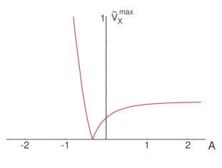
Figure 4: Dependence of $\tilde{V}_{X}^{\rm max}$ on $A$. At $A=7/3$, $\tilde{V}_{X}^{\rm max}=(3/5)^{7/3}\approx 0.3$, at $A=-7/3$, $\tilde{V}_{X}^{\rm max}=3^{7/3}\approx 13$, and the zero is at $A=-1/3$.

The maximal value that $V_{X}$ can assume is obtained when all $\tilde{N}_{j}=1$:

$$V_{X}^{\rm max}=c_{2}^{7/3}\prod_{j}a_{j}^{a_{j}}|h_{j}|^{a_{j}}\equiv c_{2}^{7/3}\prod_{j}a_{j}^{a_{j}}\,\tilde{V}_{X}^{\rm max}.$$ (4.36)

Here we isolated the $\vec{m}$-dependent product $\prod_{j}|h_{j}|^{a_{j}}$:

$$\tilde{V}_{X}^{\rm max}=\bigl{|}\frac{3}{4}+H\bigr{|}^{\frac{7}{6}+\frac{A}{2}}\,\bigl{|}\frac{3}{4}-H\bigr{|}^{\frac{7}{6}-\frac{A}{2}}.$$ (4.37)

The variation of $V_{X}^{\rm max}$ over different choices of $\vec{m}$ is entirely given by the dependence of this function on $A=\vec{a}\cdot\vec{m}$. This is shown in fig. 4.

When we take all $a_{i}=7/3n$, and we consider say the susy case $m_{i}=+1$ so $h_{i}=3/5$, (4.36) becomes

$$V_{X}^{\rm max}|_{\rm susy}=\biggl{(}\frac{7\,c_{2}}{5\,n}\biggr{)}^{7/3},$$ (4.38)

which is similar to the toy model result (3.33).

Using the usual continuum approximation for the fluxes, it is possible to get explicit expressions for the volume distribution of vacua at fixed $\vec{m}$. Taking as example again the case $a_{i}=7/3n$, we show in appendix C that for $v\equiv V_{X}/V_{X}^{\rm max}\leq 1$, at fixed $\vec{m}$ (or fixed $A$), the vacuum number density is

$$d{\cal N}_{A}[v]=\frac{\left(\frac{3n}{7}\right)^{n}}{(n-1)!}(-\ln v)^{n-1}\,v^{-\frac{3n}{7}-1}\,dv.$$ (4.39)

Therefore the total number of such vacua with $V_{X}\geq V_{*}$ goes as $V_{*}^{-3n/7}$, in agreement with the general estimates of section 3.3. Note that in addition here, the density of vacua vanishes to order $(n-1)$ near the cutoff $v=1$.

Thus, in accordance with general expectations, we see that large volumes are strongly suppressed, and more so when there are more moduli.

Analogous considerations can be made about the distribution of cosmological constants at fixed $\vec{m}$:

$$\Lambda=\frac{c_{2}^{2}\,E}{48\pi V_{X}^{3}},$$ (4.40)

with $E(A)$ as defined in section 4.1. Clearly, the distribution of $\Lambda$ is completely determined by the distribution of $V_{X}$. Thus, because large volumes are suppressed, we see that small cosmological constants are suppressed. In particular there is a lower bound on $|\Lambda|$:

$$|\Lambda|_{\rm min}=\frac{1}{48\pi}\,c_{2}^{-5}\prod_{j}a_{j}^{-3a_{j}}\,\frac{E}{(\tilde{V}_{X}^{\rm max})^{3}}=\frac{1}{48\pi}\,c_{2}^{-5}\prod_{j}a_{j}^{-3a_{j}}\,\tilde{\Lambda}$$ (4.41)

with $\tilde{\Lambda}$ as given by (4.19) and plotted in figure 2.

4.4.2 All $\vec{m}$

So far in this section, we have studied distributions at fixed $\vec{m}$, or equivalently at fixed $A$. To get complete statistics of all vacua, we need to combine these results with the distribution of solutions over values of $A$.

One general observation one can make is that since there are no metastable vacua at $A\leq-1/3$, the largest possible volume of a metastable vacuum is obtained at $A=7/3$ (and $N_{i}=1$), the supersymmetric solution. This can be seen from fig. 4. Therefore, the maximal volume for a metastable vacuum is $c_{2}^{7/3}\,\prod_{j}a_{j}^{a_{j}}\,(3/5)^{7/3}$. It is not hard to show further that $(7/3n)^{7/3}\leq\prod_{j}a_{j}^{a_{j}}\leq(7/3)^{7/3}$. The former corresponds to all $a_{i}$ equal, the latter to the limiting case $a_{i}\to 0$ for all but one $a_{i}$. Similar considerations hold for the cosmological constant. Thus we arrive at the result that for our ensembles:

$$V_{X}\leq 2.2\,c_{2}^{7/3}\,\hat{n}^{-7/3},\qquad|\Lambda|\geq 2.3\times 10^{-4}\,c_{2}^{-5}\,\hat{n}^{7}$$ (4.42)

where $1\leq\hat{n}\leq n$.

To get more refined results on the actual distributions, we need the precise distribution of solutions over $A$. This depends on the values of $a_{i}$. When all $a_{i}=7/3n$ for example, the distribution is binomial, peaked around $A=0$, which for sufficiently large $n$ is well approximated by the normal distribution given in (4.20). When all $a_{i}$ are approximately equal, the distribution will still be approximately binomial, and (4.20) is still a good approximation for large $n$. When say $a_{1}=1$ and all other $a_{i}=4/3n$ with $n$ large, the distribution will have two peaks, one at $A=1$, corresponding to $m_{1}=+1$, and the other one at $A=-1$, corresponding to $m_{1}=-1$. In the following we will work with the distribution given in (4.20).

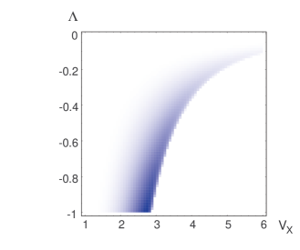
Figure 5: Density plot of the joint distribution of AdS vacua over $V_{X}$ and $\Lambda$, for $c_{2}=100$, $n=20$.

The joint distribution for $A$ and $V_{X}$ is then given by multiplying the distributions (4.20) and (4.39). Note that (4.39) depends on $A$ through $V_{X}^{\rm max}$. One can also change variables from $A$ to $E$ and thus write down a joint distribution for $E$ and $V_{X}$, or equivalently (and physically more relevantly) for $\Lambda$ and $V_{X}$, as we did for the Freund-Rubin ensemble. The explicit expressions are not very illuminating, so we will not get into details here. An example is plotted in fig. 5.

Clearly, $V_{X}$ and $\Lambda$ are correlated, as in the Freund-Rubin case. This follows directly of course from the relation $\Lambda\sim E/V_{X}^{3}$. In particular given one variable, we get a roughly Gaussian distribution of the other variable. Qualitatively this is somewhat similar to our Freund-Rubin ensemble (compare with fig. 1), although the details are different. For example in the Freund-Rubin case, at fixed $\Lambda$, the vacua accumulate near the lower bound on $V_{X}$, whereas in the $G_{2}$ case they accumulate near the upper bound. Without constraint on $\Lambda$ this gets reversed for both.

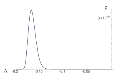
Figure 6: Distribution of cosmological constants $d{\cal N}=\rho(\Lambda)\,d\Lambda$. Here we took $a_{i}=7/3n$, $n=50$, $c_{2}=100$, and we restricted to stable vacua with $V_{X}\geq 5$.

Finally, one can get the distribution of cosmological constants for vacua with volume above some cutoff value by integrating the joint density over $V_{X}$. Again for the case with all $a_{i}=7/3n$, we obtain the distribution for $\Lambda$ shown in fig. 6 for $n=50$, $c_{2}=100$ and $V_{X}\geq 5$. The cutoff at smaller values of $|\Lambda|$ appears because of the lower cutoff we impose on the volume; the lower we take the volume cutoff, the lower the value of $\Lambda$ at which the density peaks. This is because $1/V_{X}^{3}$ sets the scale for $\Lambda$. The cutoff for small $|\Lambda|$ appears because the ensmemble does not contain vacua with arbitrarily large volume, as discussed at length before.

4.5 Supersymmetry breaking scales

Let us consider the distribution of the supersymmetry breaking scale, which for a fixed $\vec{m}$ is given by

$$M_{{\rm susy}(\vec{m})}^{2} = \left(\sqrt{e^{K}g^{i\bar{j}}DW_{i}\overline{DW_{j}}}\right)_{\vec{m}}$$ (4.43)

$$= \frac{c_{2}}{(48\pi)^{1/2}}\frac{G_{\vec{m}}^{1/2}}{V_{X}^{3/2}}$$

where

$$G_{\vec{m}}\equiv\left(\frac{7}{3}+\frac{9}{4}A^{2}\right)H^{2}+\frac{15}{8}AH+\frac{21}{64}$$ (4.44)

$G_{\vec{m}}$ is a decreasing function of $A$, which is positive for $-\frac{7}{3}\leq A<\frac{7}{3}$ and zero in the supersymmetric solution ($A=\frac{7}{3}$).

We see that the expression for $M_{\rm susy}^{4}$ is the same as that of the cosmological constant, but with $G_{\vec{m}}$ instead of $E_{\vec{m}}$. So the distribution of the supersymmetry breaking scale at fixed $\vec{m}$ is very similar to that of the cosmological constant:

• it is completely determined by the volume distribution;

• low supersymmetry breaking scales are suppressed (in line with the general expectations of section 3.6 );

• $M_{\rm susy}^{2}$ has a lower bound given by

  $$(M_{\rm susy}^{2})_{\rm min}=\frac{1}{(48\pi)^{1/2}}\,c_{2}^{-5/2}\prod_{j}a_{j}^{-3a_{j}/2}\,\frac{G^{1/2}}{(\tilde{V}_{X}^{\rm max})^{3/2}}$$ (4.45)

  with $\tilde{V}_{X}^{\rm max}$ defined in (4.37).

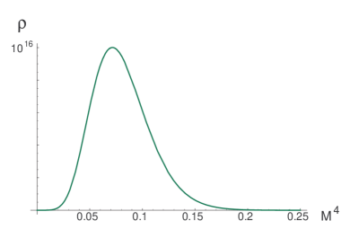
Figure 7: Distribution of supersymmetry breaking scales $d{\cal N}=\rho(M^{4})\,dM^{4}$, with $M\equiv M_{susy}/m_{p}$. Here we took $a_{i}=7/3n$, $n=50$, $c_{2}=100$, and we restricted to stable vacua with $V_{X}\geq 5$.

As for the $V_{X}$ and $\Lambda$ distributions, in order to get the complete statistic of all vacua, we need to consider the distribution of solutions over $A$, which depends on the $a_{i}$’s. Similar to what we did for $\Lambda$ in the previous subsection, we can compute the distribution of $\Lambda$ for vacua with volume bounded by some lower cutoff. This is illustrated in fig. 7. The cutoff at large values of $M_{\rm susy}$ appears because of the lower cutoff we impose on the volume, again because $1/V_{X}^{3}$ sets the scale for $M_{\rm susy}^{4}$. The lower cutoff is there because large volumes are absent.

5 Conclusions and Discussion

The potential importance of the emerging ideas surrounding the landscape, e.g. for the notion of naturalness, is clear. These ideas should therefore be tested both experimentally by verifying specific predictions and theoretically within the framework of string theory. To make progress in the latter, one should further scrutinize the proposed ensembles of string theory vacua, to establish whether or not these vacua truly persist after taking into account the full set of subtle consistency requirements, quantum corrections, and cosmological constraints [31]. Parallel to that one should develop techniques to analyze large classes of (potential) vacua without actually having to go through their detailed constructions. Only with both efforts combined can one hope to get to a satisfactory analysis of the implications of the landscape picture within string theory. If nothing else, the latter program will teach us a lot about what kind of physics is possible in string theory and assist in guiding explicit model builders, as our example in the introduction demonstrates.

The focus of our paper has been on the second program. To this end, we analyzed the statistics of Freund-Rubin and $G_{2}$ flux compactifications of $M$ theory, and compared this to known IIB results.

The statistics of Freund-Rubin vacua is very different from that of flux compactifications on special holonomy manifolds. Most notably, they can have arbitrarily high compactification volume, and accumulate near zero cosmological constant. On the other hand, these vacua typically do not have a large gap between the KK scale and the four dimensional AdS curvature scale, so they are not really compactifications in the usual sense. This is no longer true [50] if (in units in which the scalar curvature is one) the Einstein metric has all length scales much smaller than 1, but it remains a challenge to construct such manifolds with more than a modest scale hierarchy. Alternatively, one can imagine adding positive energy sources to lift the cosmological constant, perhaps even to small positive values, but no viable controlled scenario that would accomplish this is presently known. The problem is clear: in order to lift the cosmological constant to a positive value, one would have to add an energy source at or near the Kaluza-Klein scale, which makes 4d effective field theory unreliable and could easily destabilize the compactification. Adding such effects could also drastically change the distributions of vacua over parameter space. Therefore, the results we obtained for Freund-Rubin vacua should not be interpreted as showing there are parts of the landscape compatible with rough observational requirements that for example strongly favor large volumes. But our results do show that this is possible in principle, and constructing Freund-Rubin-like vacua which overcome the above mentioned problems would therefore be all the more interesting.

The statistics of $G_{2}$ flux vacua has a number of universal features. One is that the distribution of vacua over moduli space is uniform with respect to the Kähler metric on moduli space. In essence, because the large volume region of moduli space is small when its dimension $b_{3}$ is large, this implies that large compactification volumes are suppressed, and strongly so if $b_{3}$ is large. In particular there is an upper bound to the volume in a given ensemble, set by the Chern-Simons invariant $c_{2}$. This is true as well for IIB flux ensembles studied thus far and for their presumed IIA mirror counterparts, where the maximal size is set by the D3 tadpole cutoff $L$. Since both the IIB and the $G_{2}$ ensembles contain flux degrees of freedom that are not dual to flux degrees of freedom in the other ensemble, but are possibly dual to discrete geometrical deformations away from special holonomy, this suggests this behavior will persist when extending the ensembles to also sample non-flux discrete compactification data away from special holonomy. Our results on Freund-Rubin vacua on the other hand show that departure from special holonomy can produce the opposite behavior. So before general conclusions can be drawn, this question needs to be investigated in more general ensembles. Since the full 10d geometries of such extended ensembles tend to be hard to describe, an effective four dimensional field theory approach, as worked out in [46] and used for example in [47] to find ${\cal N}=2$ IIA flux vacua, would probably be the best way to make progress in this direction.

Essentially because of the limited discrete tunability of $G_{2}$ flux vacua, the scale of the cosmological constant is set by the volume, $\Lambda\sim m_{p}^{4}/V^{3}$. Since large volumes are strongly suppressed at large $b_{3}$, it follows that small cosmological constants are strongly suppressed as well. This contrasts with type IIB ensembles, where the distribution of cosmological constants is uniform near zero. Similarly, the scale of supersymmetry breaking is set by $m_{p}^{2}/V^{3/2}$, so small supersymmetry breaking scales are suppressed. For $b_{3}$ not too small, this remains true even when taking into account tuning of Higgs mass and cosmological constants. F-breaking IIB flux vacua similarly favor high susy breaking scales, although $M^{2}_{\rm susy}$ can be tuned to be small there, and the suppression was found to be independent of the number of moduli in the regime where $M_{\rm susy}^{2}$ is much smaller than the fundamental scale [20]. It is plausible that extending the $G_{2}$ ensembles as discussed above would allow the supersymmetry breaking scale to be tuned small as well, reproducing the statistics of the generic ensembles of [20] in this regime, but this would still favor higher scales. Another generalization which we did not consider in this work is D-term supersymmetry breaking. We refer to [20] for further discussion of this possibility.

The next step to take would be to embed standard-like models in these (and other) flux ensembles, and study the distributions of various couplings. In particular it would be interesting to analyze the impact of environmental constraints on these distributions, to see if for example the split supersymmetry scenario of [38] naturally emerges, and if these ensembles are “friendly neighborhoods” of the landscape, in the terminology of [28]. To get an idea of the possibly very important role of environmental constraints in determining the physically relevant distributions, consider the “atomic principle” [38], which, when the light Yukawa couplings are fixed, constrains the weak scale $v$ to lie in a narrow window set by the (naturally small) QCD scale. More generally, leaving the Yukawa couplings $y$ arbitrary, it is actually the combination $yv$ which is constrained to lie in a narrow window, so the environmental explanation of the smallness of $v$ would be lost if $y$ scans densely around zero in the ensemble. Now, in $M$ theory vacua where the quarks and leptons are localized at isolated points in the extra dimensions [52, 53], the Yukawa couplings are generated by $M$2-brane instantons wrapping 3-cycles containing these points [53] and are therefore roughly of order $e^{-s}$, with $s$ one of the geometric moduli we have worked with throughout our analysis. The values of $s$ vary over the ensemble, so the Yukawas scan many orders of magnitude [62], but not uniformly around zero: as we have seen, large values of $s$ are suppressed and bounded above. Hence these ensembles are precisely of the kind envisioned in [28] that would be sufficiently friendly to allow the atomic principle to play a role in explaining the smallness of $v$. In fact, it may even play a role in explaining the smallness of the light Yukawas. A priori, these ensembles favor smaller $s$ and therefore larger Yukawas. However, with smaller Yukawas, the Higgs is allowed to vary over a wider range. Taking this into account gives an enhancement of order $e^{s}$ in the number of vacua compatible with the atomic principle, and this could easily overpower the a priori $1/s^{k}$ suppression of large $s$. Apart from illustrating the potential power of environmental principles, this also shows that such constraints can strongly influence the physically relevant distributions. We plan to return to these and other issues in future work.

Acknowledgements

We would like to thank Nima Arkani-Hamed, Michael Dine, Mike Douglas, Shamit Kachru, Greg Moore, Sav Sethi and Eva Silverstein for valuable discussions.

Appendix A Normalizations

We defined

$$K=-3\ln\left(4\pi^{1/3}V_{X}\right);\qquad W_{flux}(z)={1\over\kappa_{4}^{3}}N_{i}z^{i}$$ (A.1)

The expression for the supergravity potential is the standard one for the case of dimensionless scalars:

$$V=\kappa_{4}^{2}\,e^{K}\,(g^{i\bar{j}}D_{i}W\bar{D}_{\bar{j}}\bar{W}-3|W|^{2})$$ (A.2)

Note that when expressed in terms of the moduli $z$, none of these effective four dimensional field theory quantities explicitly contains the fundamental scale $\ell_{M}$, only the four dimensional Planck scale $\kappa_{4}$, which is the directly measurable scale in four dimensions. To check our normalizations, it is sufficient to verify the tension of a domain wall corresponding to an M5 brane wrapped around a supersymmetric 3-cycle $\Sigma$, which is Poincaré dual to the jump in flux $\Delta G$ across the wall. Let’s take $C=0$ for simplicity. In the supergravity theory, we have

$$T_{DW} = 2e^{K/2}|\Delta W|$$

$$= {2\over V_{X}^{3/2}8\sqrt{\pi}\kappa_{4}^{3}}|\Delta N_{i}z^{i}|$$

$$= {2\pi\over(4\pi\kappa_{4}^{2}V_{X})^{3/2}\ell_{M}^{3}}|\int_{\Sigma}\varphi|$$

$$= {2\pi\over\ell_{M}^{6}}\mbox{vol}(\Sigma)$$

$$= T_{5}\mbox{vol}(\Sigma),$$

which is indeed the correct expression in $M$ theory.

Appendix B Stability analysis

The sign of the potential for a particular solution depends on the sign of $E$, with $E$ as defined in section 4.1. It is negative when $A\equiv\vec{a}\cdot\vec{m}>-1/3$ and it is positive when $A<-1/3$. We discuss these cases separately.

B.1 AdS vacua

An AdS critical point $s^{0}$ does not have to be a local minimum to be perturbatively stable. It suffices that the eigenvalues of the Hessian of $V$ are not too negative compared to the cosmological constant, and more precisely that Breitenlohner-Freedman bound is satisfied [60]:

$$\hat{\partial}_{i}\hat{\partial}_{j}V(s^{0})-\frac{3}{2}V(s^{0})\delta_{ij}\geq 0,$$ (B.1)

i.e. this matrix should be positive definite.

The derivatives are done with respect to the canonically normalized scalars. The relevant kinetic term expanded around the critical point $s^{0}$ is (in 4d Planck units):

$$g_{i\bar{j}}\partial_{\mu}z^{i}\partial^{\mu}\bar{z}^{\bar{j}} = \sum_{i}\frac{3a_{i}}{4(s_{i}^{0})^{2}}(\partial_{\mu}t_{i}\partial^{\mu}t_{i}+\partial_{\mu}s_{i}\partial^{\mu}s_{i})+\cdots$$ (B.3)

$$\equiv\sum_{i}\frac{1}{2}(\partial_{\mu}\hat{t}_{i}\partial^{\mu}\hat{t}_{i}+\partial_{\mu}\hat{s}_{i}\partial^{\mu}\hat{s}_{i})+\cdots$$

Hence the canonically normalized scalars are

$$\hat{s}_{i}=\sqrt{\frac{3a_{i}}{2}}\,\frac{s_{i}}{s_{i}^{0}}.$$ (B.4)

With this redefinition, the condition (B.1) becomes

$$\frac{2}{3}\frac{s_{i}^{0}s_{j}^{0}}{\sqrt{a_{i}a_{j}}}\partial_{i}\partial_{j}V(s^{0})-\frac{3}{2}V(s^{0})\delta_{ij}\geq 0$$ (B.5)

where

$$\partial_{i}\partial_{j}V = \frac{c_{2}^{2}}{48\pi V_{X}^{3}}\left(\frac{3a_{i}a_{j}}{s_{i}s_{j}}\left(3E-2(\nu_{i}^{2}s_{i}^{2}+\nu_{j}^{2}s_{j}^{2})+3(\nu_{i}s_{i}+\nu_{j}s_{j})\right)\right.$$ (B.6)

$$+\left.\frac{a_{i}}{s_{i}^{2}}\left(3E+2\nu_{i}^{2}s_{i}^{2}\right)\delta_{ij}\right)$$

$$V = \frac{c_{2}^{2}}{48\pi V_{X}^{3}}E$$

$$E = 3+\sum_{j=1}^{n}a_{j}\nu_{j}s_{j}(\nu_{j}s_{j}-3)$$

By substituting these expressions in (B.5), using the variables $h_{i}=\nu_{i}s_{i}$ and factoring out the common positive term $\frac{c_{2}^{2}}{48\pi V_{X}^{3}}$, the stability condition becomes:

$$M_{ij}\equiv\sqrt{a_{i}a_{j}}(6E-4(h_{i}^{2}+h_{j}^{2})+6(h_{i}+h_{j}))+\delta_{ij}(\frac{E}{2}+\frac{4}{3}h_{i}^{2})\geq 0$$ (B.7)

where

$$E=\frac{2}{3}H^{2}-\frac{3}{8}=-\frac{3}{100}\left(5-9A^{2}+3A\sqrt{9A^{2}+15}\right).$$ (B.8)

Let us evaluate (B.7) on our solutions.

• supersymmetric solution:

  $$\mathbf{M}=\frac{54}{25}\,\mathbf{q}+\frac{3}{10}\,\mathbf{1}$$ (B.9)

  where $q_{ij}=\sqrt{a_{i}a_{j}}$ is a rank$=1$ positive definite matrix. We see that $\mathbf{M}\geq 0$ and so that the supersymmetric solution is always stable.

• Other AdS ($A>-1/3$) solutions:

  $$\mathbf{M}=Q\,\mathbf{q}+S\,\mathbf{1}+T\,\mathbf{t}$$ (B.10)

  where

  $$Q=-6E,\qquad S=\frac{E}{2}+\frac{4}{3}\left(H+\frac{3}{4}\right)^{2},\qquad T=-4H$$ (B.11)

  $$t_{ij}=\frac{(1-m_{i})}{2}\delta_{ij}.$$ (B.12)

  The following relations are valid: $Q>0$, $T>0$ and $S+T>0$; so $Q\,\mathbf{q}$ and $T\,\mathbf{t}$ are always positive definite. $S$ has no definite sign. We have two cases:

  1. when $A\geq\frac{1}{3}$, $S\geq 0$; then $S\,\mathbf{1}$ and consequently $\mathbf{M}$ is positive, and the corresponding solutions are perturbatively stable;

  2. when $-\frac{1}{3}<A<\frac{1}{3}$, $S<0$; in this case the $\mathbf{M}$ matrix is not positive definite when $\vec{m}$ has more than one entry equal to $+1$ and the corresponding solutions are not stable. Actually, if $m_{h}=+1$ and $m_{k}=+1$, $\mathbf{M}$ has the $2\times 2$ minor

     $$Q\left(\begin{array}[]{cc}a_{h}&\sqrt{a_{h}a_{k}}\\ \sqrt{a_{h}a_{k}}&a_{k}\end{array}\right)+\left(\begin{array}[]{cc}S&0\\ 0&S\end{array}\right)$$ (B.13)

     which has $S<0$ as one of the two egenvalues.
     On the other hand, when $\vec{m}$ has exactly one entry equal to $+1$, the solution is a local minimum and so it is stable.

Let us prove that when $A>-\frac{1}{3}$ and exactly one $m_{i}$ is equal to $+1$, the corresponding solution is a local minimum.

Without loss of generality we choose $i=1$. $\partial^{2}V$ is proportional to $\mathbf{\hat{M}}\equiv\mathbf{q}+\frac{S^{\prime}}{Q}\mathbf{1}+\frac{T}{Q}\mathbf{t}$, where $S^{\prime}\equiv S+\frac{3}{2}E$ is negative for all considered values of $A$. Let us call $B=\frac{S^{\prime}+T}{Q}>0$, $C=-\frac{S^{\prime}}{Q}>0$, $v_{i}=\sqrt{a_{i}}$. So $|v|^{2}=7/3$, $v_{1}>1$ and

$$\mathbf{\hat{M}}=v\,v^{t}+\left(\begin{array}[]{cccc}-C&&&\\ &B&&\\ &&\ldots&\\ &&&B\end{array}\right)$$ (B.14)

By direct study of its eigenvalues, it can be shown that this matrix is positive definite for $n=2$. Now we prove by induction that this matrix is positive definite for each $n$.

Let us assume that $\forall y\in\mathbb{R}^{n}$

$$y^{t}\mathbf{\hat{M}}_{n}y=(v_{1}y_{1}+\tilde{v}\cdot\tilde{y})^{2}+B\tilde{y}^{2}-Cy_{1}^{2}>0$$ (B.15)

where $V=(V_{1},\tilde{V})$. Let $u$ be the extension of $v\in\mathbb{R}^{n}$ to $\mathbb{R}^{n+1}$, i.e. $u_{i}=\sqrt{a_{i}}$. Then $\forall x\in\mathbb{R}^{n+1}$ there exists $y\in\mathbb{R}^{n}$, such that

$$y_{1}=x_{1} \tilde{y}\cdot\tilde{v}=\tilde{x}\cdot\tilde{u} \tilde{y}^{2}=\tilde{x}^{2}$$ (B.16)

It follows that

$$x^{t}\mathbf{\hat{M}}_{n+1}x=(u_{1}x_{1}+\tilde{u}\cdot\tilde{x})^{2}+B\tilde{x}^{2}-Cx_{1}^{2}>0$$ (B.17)

QED.

B.2 dS vacua

The solutions with positive potential (i.e. $A<-1/3$) must be local minima to be metastable, and so the matrix $\mathbf{M^{\prime}}\equiv Q\,\mathbf{q}+S^{\prime}\,\mathbf{1}+T\,\mathbf{t}$ (in the notations introduced in the first part of this appendix) must be positive definite. We now show that this is never the case.

We have $\mathbf{q}=vv^{t}$, where $v_{i}=\sqrt{a_{i}}$ and so $|v|^{2}=7/3$. Let us consider the $n\times n$ matrix defined by $\mathbf{M^{\prime\prime}}\equiv Q\,\mathbf{q}+S^{\prime}\,\mathbf{1}+T\,\mathbf{1}$. If $\mathbf{M^{\prime}}$ is positive definite then $\mathbf{M^{\prime\prime}}$ is positive too. Clearly, its eigenvalues are $S^{\prime}+T$, which is positive for $A<-1/3$, and

$$\lambda=Q|v|^{2}+S^{\prime}+T=\frac{7}{3}Q+S^{\prime}+T.$$ (B.18)

By studying $\lambda$ as a function of $A$, one finds that it is positive for $A>-17/21$. So $\mathbf{M^{\prime\prime}}$ is not positive definite for $A<-17/21\approx-0.8095$ and so $\mathbf{M^{\prime}}$ is not positive for the same values.

Moreover one can study the $k\times k$ submatrix of $\mathbf{M^{\prime}}$ obtained by restriction to the subspace on which $m_{j}=+1$ ($k$ is the number of such $m_{j}$’s). This is equal to $Q\,vv^{t}+S^{\prime}\,\mathbf{1}_{k}$, where we are considering only $v_{j}$ corresponding to $m_{j}=+1$. Its eigenvalues are $S^{\prime}$, which is positive for $A<-1/3$, and

$$\mu=Q\sum_{i=1}^{n}\frac{(1+m_{i})}{2}a_{i}+S^{\prime}=Q(\frac{7}{6}+\frac{A}{2})+S^{\prime}.$$ (B.19)

By studing $\mu$ as a function of $A$, one finds that it is negative for $\alpha<A<-\frac{1}{3}$, where $\alpha\approx-1.44075$. For these values of $A$ we have a nonpositive minor and so $\mathbf{M^{\prime}}$ is not positive definite.

By combining these two results, we see that for no value of $A<-\frac{1}{3}$ the corresponding solution is a local minimum. Thus, all dS critical points are unstable in our model ensembles.

Appendix C Volume distribution

Here we give details on how to arrive at the distribution (4.39) of volumes $v=V_{X}/V_{X}^{\rm max}$ when all $a_{i}=a=7/3n$:

$$d{\cal N}[v]/dv = \sum_{\tilde{N_{i}}\geq 1}\delta(v-\prod_{i}\tilde{N}_{i}^{-a})$$

$$\approx \int_{\tilde{N}_{i}\geq 1}d^{n}\tilde{N}\,\delta(v-\prod_{i}\tilde{N}_{i}^{-a})$$

$$= \int_{U_{i}\geq 0}d^{n}U\,e^{\sum_{j}U_{j}}\,\delta(v-e^{-a\sum_{j}U_{j}})$$

$$= \frac{1}{a}\,e^{-(1+a)\frac{\ln v}{a}}\int d^{n}U\,\delta(\sum_{j}U_{j}+\frac{\ln v}{a})$$

$$= \frac{1}{a}\,v^{-(1+1/a)}\,\frac{(-\frac{\ln v}{a})^{n-1}}{(n-1)!}\,\Theta(1-v)$$

$$= \frac{\left(\frac{3n}{7}\right)^{n}}{(n-1)!}(-\ln v)^{n-1}\,v^{-\frac{3n}{7}-1}\,\Theta(1-v)$$

References

- [1] N. Arkani-Hamed, S. Dimopoulos and G. R. Dvali, “The hierarchy problem and new dimensions at a millimeter,” Phys. Lett. B 429 (1998) 263 [arXiv:hep-ph/9803315]. I. Antoniadis, N. Arkani-Hamed, S. Dimopoulos and G. R. Dvali, “New dimensions at a millimeter to a Fermi and superstrings at a TeV,” Phys. Lett. B 436 (1998) 257 [arXiv:hep-ph/9804398].
- [2] S. Kachru, R. Kallosh, A. Linde and S. P. Trivedi, “De Sitter vacua in string theory,” Phys. Rev. D 68 (2003) 046005 [arXiv:hep-th/0301240].
- [3] B. S. Acharya, “A moduli fixing mechanism in theory,” arXiv:hep-th/0212294.
- [4] R. Bousso and J. Polchinski, “Quantization of four-form fluxes and dynamical neutralization of the cosmological constant,” JHEP 0006, 006 (2000) [arXiv:hep-th/0004134].
- [5] M. R. Douglas, “The statistics of string / theory vacua,” JHEP 0305, 046 (2003) [arXiv:hep-th/0303194].
- [6] S. Ashok and M. R. Douglas, “Counting flux vacua,” JHEP 0401, 060 (2004) [arXiv:hep-th/0307049].
- [7] M. R. Douglas, “Statistics of string vacua,” arXiv:hep-ph/0401004.
- [8] M. R. Douglas, B. Shiffman and S. Zelditch, “Critical points and supersymmetric vacua,” Commun. Math. Phys. 252, 325 (2004) [arXiv:math.cv/0402326].
- [9] F. Denef and M. R. Douglas, “Distributions of flux vacua,” JHEP 0405, 072 (2004) [arXiv:hep-th/0404116].
- [10] A. Giryavets, S. Kachru and P. K. Tripathy, “On the taxonomy of flux vacua,” JHEP 0408, 002 (2004) [arXiv:hep-th/0404243].
- [11] M. R. Douglas, B. Shiffman and S. Zelditch, “Critical points and supersymmetric vacua, II: Asymptotics and extremal metrics,” arXiv:math.cv/0406089.
- [12] A. Misra and A. Nanda, “Flux vacua statistics for two-parameter Calabi-Yau’s,” arXiv:hep-th/0407252.
- [13] M. R. Douglas, “Basic results in vacuum statistics,” Comptes Rendus Physique 5, 965 (2004) [arXiv:hep-th/0409207].
- [14] J. P. Conlon and F. Quevedo, “On the explicit construction and statistics of Calabi-Yau flux vacua,” JHEP 0410 (2004) 039 [arXiv:hep-th/0409215].
- [15] J. Kumar and J. D. Wells, “Landscape cartography: A coarse survey of gauge group rank and stabilization of the proton,” Phys. Rev. D 71, 026009 (2005) [arXiv:hep-th/0409218].
- [16] O. DeWolfe, A. Giryavets, S. Kachru and W. Taylor, “Enumerating Flux Vacua with Enhanced Symmetries,” [arXiv:hep-th/0411061].
- [17] L. Susskind, “Supersymmetry breaking in the anthropic landscape,” arXiv:hep-th/0405189.
- [18] M. R. Douglas, “Statistical analysis of the supersymmetry breaking scale,” arXiv:hep-th/0405279.
- [19] M. Dine, E. Gorbatov and S. Thomas, “Low energy supersymmetry from the landscape,” arXiv:hep-th/0407043.
- [20] F. Denef and M. R. Douglas, “Distributions of nonsupersymmetric flux vacua,” arXiv:hep-th/0411183.
- [21] M. Dine, “Supersymmetry, naturalness and the landscape,” arXiv:hep-th/0410201.
- [22] M. Dine, D. O’Neil and Z. Sun, “Branches of the Landscape,” arXiv:hep-th/0501214.
- [23] T. P. T. Dijkstra, L. R. Huiszoon and A. N. Schellekens, “Supersymmetric standard model spectra from RCFT orientifolds,” arXiv:hep-th/0411129.
- [24] R. Blumenhagen, F. Gmeiner, G. Honecker, D. Lust and T. Weigand, “The statistics of supersymmetric D-brane models,” arXiv:hep-th/0411173.
- [25] G. Dvali, “Large hierarchies from attractor vacua,” arXiv:hep-th/0410286.
- [26] K. R. Dienes, E. Dudas and T. Gherghetta, “A calculable toy model of the landscape,” arXiv:hep-th/0412185.
- [27] M. Tegmark, “What does inflation really predict?,” arXiv:astro-ph/0410281.
- [28] N. Arkani-Hamed, S. Dimopoulos and S. Kachru, “Predictive landscapes and new physics at a TeV,” arXiv:hep-th/0501082.
- [29] E. Silverstein, “Counter-intuition and scalar masses,” arXiv:hep-th/0407202.
- [30] T. Banks, M. Dine and E. Gorbatov, “Is there a string theory landscape?,” JHEP 0408 (2004) 058 [arXiv:hep-th/0309170].
- [31] T. Banks, “Landskepticism or why effective potentials don’t count string models,” arXiv:hep-th/0412129.
- [32] E. Witten, “Deconstruction, G(2) holonomy, and doublet-triplet splitting,” arXiv:hep-ph/0201018; T. Friedmann and E. Witten, “Unification scale, proton decay, and manifolds of G(2) holonomy,” Adv. Theor. Math. Phys. 7 (2003) 577 [arXiv:hep-th/0211269].
- [33] B. S. Acharya, “Observations on the space of four dimensional string and theory vacua,” arXiv:hep-th/0406228.
- [34] P. G. O. Freund and M. A. Rubin, “Dynamics Of Dimensional Reduction,” Phys. Lett. B 97, 233 (1980).
- [35] S. Weinberg, “Anthropic Bound On The Cosmological Constant,” Phys. Rev. Lett. 59, 2607 (1987).
- [36] A. Vilenkin, “Predictions from quantum cosmology,” Phys. Rev. Lett. 74, 846 (1995) [arXiv:gr-qc/9406010].
- [37] V. Agrawal, S. M. Barr, J. F. Donoghue and D. Seckel, “The anthropic principle and the mass scale of the standard model,” Phys. Rev. D 57, 5480 (1998) [arXiv:hep-ph/9707380].
- [38] N. Arkani-Hamed and S. Dimopoulos, “Supersymmetric unification without low energy supersymmetry and signatures for fine-tuning at the LHC,” arXiv:hep-th/0405159.
- [39] N. Arkani-Hamed, S. Dimopoulos, G. F. Giudice and A. Romanino, “Aspects of split supersymmetry,” arXiv:hep-ph/0409232.
- [40] S. Gukov, C. Vafa and E. Witten, “CFT’s from Calabi-Yau four-folds,” Nucl. Phys. B 584 (2000) 69 [Erratum-ibid. B 608 (2001) 477] [arXiv:hep-th/9906070].
- [41] F. Denef, M. R. Douglas and B. Florea, “Building a better racetrack,” JHEP 0406, 034 (2004) [arXiv:hep-th/0404257].
- [42] V. Balasubramanian, P. Berglund, J. Conlon and F. Quevedo, “Systematics of Moduli Stabilisation in Calabi-Yau Flux Compactifications,” arXiv:hep-th/0502058.
- [43] V. Balasubramanian and P. Berglund, “Stringy corrections to Kaehler potentials, SUSY breaking, and the cosmological constant problem,” JHEP 0411, 085 (2004) [arXiv:hep-th/0408054].
- [44] F. Denef and M. Douglas, unpublished.
- [45] A. Saltman and E. Silverstein, “A new handle on de Sitter compactifications,” arXiv:hep-th/0411271.
- [46] T. Grimm and J. Louis, “The effective action of Type IIA orientifolds,” arxiv:hep-th/0412277
- [47] S. Kachru and A. K. Kashani-Poor, “Moduli potentials in type IIA compactifications with RR and NS flux,” arXiv:hep-th/0411279.
- [48] S. Kachru, M. B. Schulz, P. K. Tripathy and S. P. Trivedi, “New supersymmetric string compactifications,” JHEP 0303 (2003) 061 [arXiv:hep-th/0211182]. M. B. Schulz, “Calabi-Yau duals of torus orientifolds,” arXiv:hep-th/0412270; S. Gurrieri, J. Louis, A. Micu and D. Waldram, “Mirror symmetry in generalized Calabi-Yau compactifications,” Nucl. Phys. B 654 (2003) 61 [arXiv:hep-th/0211102].
- [49] M. J. Duff, B. E. W. Nilsson and C. N. Pope, “Spontaneous Supersymmetry Breaking By The Squashed Seven Sphere,” Phys. Rev. Lett. 50 (1983) 2043.
- [50] B. S. Acharya, F. Denef, C. Hofman and N. Lambert, “Freund-Rubin revisited,” arXiv:hep-th/0308046.
- [51] E. Witten, “Fermion Quantum Numbers In Kaluza-Klein Theory,” PRINT-83-1056 (PRINCETON)
- [52] M. Atiyah and E. Witten, “ theory dynamics on a manifold of G(2) holonomy,” Adv. Theor. Math. Phys. 6 (2003) 1 [arXiv:hep-th/0107177].
- [53] B. Acharya and E. Witten, “Chiral fermions from manifolds of G(2) holonomy,” arXiv:hep-th/0109152.
- [54] C. Beasley and E. Witten, “A note on fluxes and superpotentials in theory compactifications on manifolds of holonomy,” JHEP 0207, 046 (2002) [arXiv:hep-th/0203061].
- [55] S. Gukov, “Solitons, superpotentials and calibrations,” Nucl. Phys. B 574, 169 (2000) [arXiv:hep-th/9911011].
- [56] B. S. Acharya and B. Spence, “Flux, supersymmetry and theory on 7-manifolds,” arXiv:hep-th/0007213.
- [57] B. S. Acharya, “ theory, Joyce orbifolds and super Yang-Mills,” Adv. Theor. Math. Phys. 3, 227 (1999) [arXiv:hep-th/9812205]; B. S. Acharya, “On realising N = 1 super Yang-Mills in theory,” arXiv:hep-th/0011089.
- [58] A. Bergman and C. P. Herzog, “The volume of some non-spherical horizons and the AdS/CFT correspondence,” JHEP 0201, 030 (2002) [arXiv:hep-th/0108020].
- [59] J. P. Gauntlett, D. Martelli, J. F. Sparks and D. Waldram, “A new infinite class of Sasaki-Einstein manifolds,” arXiv:hep-th/0403038.
- [60] P. Breitenlohner and D. Z. Freedman, “Positive Energy In Anti-De Sitter Backgrounds And Gauged Extended Supergravity,” Phys. Lett. B 115, 197 (1982).
- [61] A. Lukas and S. Morris, “Moduli Kaehler potential for theory on a G(2) manifold,” Phys. Rev. D 69, 066003 (2004) [arXiv:hep-th/0305078].
- [62] B. S. Acharya, “Compactification with flux and Yukawa hierarchies,” arXiv:hep-th/0303234.