Accelerating universes driven by bulk particles

Abstract

We consider our universe as a 3d domain wall embedded in a 5d dimensional Minkowski space-time. We address the problem of inflation and late time acceleration driven by bulk particles colliding with the 3d domain wall. The expansion of our universe is mainly related to these bulk particles. Since our universe tends to be permeated by a large number of isolated structures, as temperature diminishes with the expansion, we model our universe with a 3d domain wall with increasing internal structures. These structures could be unstable 2d domain walls evolving to fermi-balls which are candidates to cold dark matter. The momentum transfer of bulk particles colliding with the 3d domain wall is related to the reflection coefficient. We show a nontrivial dependence of the reflection coefficient with the number of internal dark matter structures inside the 3d domain wall. As the population of such structures increases the velocity of the domain wall expansion also increases. The expansion is exponential at early times and polynomial at late times. We connect this picture with string/M-theory by considering BPS 3d domain walls with structures which can appear through the bosonic sector of a five-dimensional supergravity theory.

I Introduction

Following the recent ideas concerning extra-dimensions nima1 ; nima2 ; rs1 ; rs2 ; kr we consider our universe as a 3d domain wall embedded in a 5d dimensional space-time. We explore some current issues of the modern cosmology such as inflation and late time accelerating universes. Accelerating expansion can be modelled by considering a dynamical cosmological constant $\Lambda$ peebles ; steinhardt in the form of a scalar field with a scalar potential and a slowly varying energy density. This idea is currently called quintessence. In this paper we show how this mechanism can appear via bulk particles collisions with domain walls. These are 3d domain walls engendering an amount of internal structures increasing with time. Such structures can be unstable 2d domain walls evolving to fermi-balls which are candidates to cold dark matter macpherson ; bazmorris . This is an interesting alternative to understand acceleration of our universe as a consequence of bulk effects. This can be relevant to reproduce accelerating universes in string/M-theory cosmology vijay ; kklt ; kklmmt . Accelerating universes require violation of the strong energy condition that is not allowed by potentials obtained through compactifications from ten/eleven-dimensional down to four-dimensional supergravity theories nogoth1 ^[1]. However, these potentials can produce BPS solitonic solutions such as a BPS 3d domain wall (3-brane) inside a bulk nunez whose dynamics between the 3-brane and particles inside the bulk can play the crucial role of giving rise to accelerating universes on a 3-brane. In other words, a brane observer can “see” a potential on a BPS 3-brane induced by bulk particles collisions. This potential unlike the potentials coming from compactifications can violate the strong energy condition and then can be suitable to realize accelerating universes. In this scenario the dark energy effect needed to drive both early and late time acceleration can be recognized as the effect of “brane dark matter” plus “bulk particle collisions.” Such particles travelling the bulk can be associated with the 3-brane fluctuations effect itself or some exotic particles. We show that this scenario can also accommodate inflation in early time cosmology. Our scenario can be considered as a new perspective to accelerating universes in braneworlds cosmology scenarios dgp ; dg ; defayet ; ac-davis .

In this paper we follow a program we have considered in several contexts mackenzie ; morris97 ; bb97 ; etbb97 ; bbb ; bazbrito ; bb2000 ; bb2001 . This program concerns the issue of localization of defects inside other defects of higher dimensions in field theory. This was inspired by the idea of superconducting cosmic strings witten85 . Essentially one considers the fact that inside, i.e., near the core of a defect, a scalar or a vector field can develop a nonzero vacuum expectation value (v.e.v.). To provide structures formation such as domain walls inside another domain wall one has to consider a theory with a $Z_{2}\times Z_{2}$ symmetry. Thus, in our analysis, the appearance of a scalar field developing a v.e.v. inside a 3d domain wall, breaks a particular $Z_{2}$ symmetry favoring the formation of another domain wall with smaller dimension. These configurations of defects inside defects in field theory have some analog in braneworlds with warped geometry where one considers 3-branes inside higher dimensional spaces such as 5d anti-de-Sitter space-time ($AdS_{5}$) rs1 ; rs2 ; kr .

We shall consider here a 3d domain wall (a thick 3-brane) with internal structure such as other domain walls. We mainly address the problem of particle collision with a 3d domain wall embedded in 5d Minkowski space-time dgp ; dg . We calculate the reflection probability of these particles by considering they collide elastically with the domain wall. As we shall see, the total mass of the domain wall does not change as the number of internal structure increases. Thus we disregard absorbtion of bulk particles and also consider these particles are hitting the 3d domain wall orthogonally, i.e., there is no tangential momentum transfer to any individual structure inside the domain wall ^[2]. In our scenario the domain wall expands as it moves along the 5d space-time, and this motion is essentially due to the total momentum transferred by bulk particles. We consider two types of 3d domain wall solutions: (i) domain walls without internal structure and (ii) domain walls with internal structure. They appear as BPS solitonic solutions of the bosonic sector of a 5d supergravity theory.

We argue that 3d domain walls with internal structure colliding with bulk scalar particles can drive inflation in early time cosmology and accelerating expansion in late time universe. (Investigations concerning accelerating universes in scenarios with S-branes inside D-branes have been considered in edels ). The expansion is controlled by the amount of internal structures that increases with the time according to a power-law. At early times the reflection probability increases exponentially and then provides an inflationary period of our universe. At very late times the reflection probability saturates to a constant leading to a universe expanding according to a quadratic-law. Accelerating expansion in our universe is in agreement with recent cosmological observational data supernovae ; Ries .

The paper is organized as in the following. In Sec. II we find 2d domain walls inside a 3d domain wall as solitonic solutions of the bosonic sector of a 5d supergravity theory. In Sec. III we present the quantum mechanics problem of bulk particles interacting with Schroedinger potentials associated with the 3d domain walls. In Sec. IV we calculate the reflection probability and identify the number of 2d domain walls as a parameter of control. The 3d domain wall expansion is explored in detail in Sec. V. Final discussions are considered in Sec. VI.

II The model: walls inside wall

We consider the bosonic scalar sector of a five-dimensional supergravity theory obtained via compactification of a higher dimensional supergravity whose Lagrangian is cv ; dwolfe ; bcy ; cvlambert ; bbn

$$e^{-1}{\cal L}_{sugra}=-\frac{1}{4}\,{M_{*}}^{3}R_{(5)}+\,G_{AB}\,\partial_{\mu}\phi^{A}\,\partial^{\mu}\phi^{B}-\frac{1}{4}\,G^{AB}\,\frac{\partial W(\phi)}{\partial\phi^{A}}\frac{\partial W(\phi)}{\partial\phi^{B}}+\frac{1}{3}\frac{1}{{M_{*}}^{3}}\,W(\phi)^{2},$$ (1)

where $G_{AB}$ is the metric on the scalar target space and $e=|\det g_{\mu\nu}|^{1/2}$. $R_{(5)}$ is the 5d Ricci scalar and $1/M_{*}$ is the five-dimensional Planck length. Below we consider the limit $M_{*}\!\gg\!1$ (with $M_{*}\ll M_{Pl}$) where five-dimensional gravity is not coupled to the scalar field. In this limit the 3-brane is a classical 3d domain wall solution embedded in a 5d Minkowski space. The 4d gravity is induced on the brane via quantum loops of matter fields confined on the brane dgp ; dg . The Standard Model particles are localized on the brane via mechanisms described in nima1 ; nima2 — see also susy1SM for realizations in string models. We also restrict the scalar manifold to two fields only, i.e., $\phi_{A}=(\phi/\sqrt{2},\chi/\sqrt{2})$.

In order to have formation of domain walls inside domain walls, we consider a supersymmetric model with two coupled real scalar fields engendering a $Z_{2}\times Z_{2}$ symmetry (for now we consider this as an exact symmetry) described by the scalar sector of the Lagrangian (1), i.e.,

$$\mathcal{L}=\frac{1}{2}\partial_{\mu}\phi\partial^{\mu}\phi+\frac{1}{2}\partial_{\mu}\chi\partial^{\mu}\chi-V(\phi,\chi),$$ (2)

where the scalar potential is given in terms of the superpotential as

$$V(\phi,\chi)=\frac{1}{2}\left(\frac{\partial W}{\partial\phi}\right)^{2}+\frac{1}{2}\left(\frac{\partial W}{\partial\chi}\right)^{2}.$$ (3)

The most general form of a superpotential engendering a $Z_{2}\times Z_{2}$ symmetry bbb is

$$W=\lambda\left(\frac{\phi^{3}}{3}-a^{2}\phi\right)+\mu\phi\chi^{2}.$$ (4)

The physical meaning of the parameters $\lambda$ and $\mu$ will become clear later as we recognize $N=\sqrt{\mu/\lambda}$ as the number of internal structures inside the 3d domain wall. Using the superpotential above gives

$$V(\phi,\chi)=\frac{1}{2}\lambda^{2}(\phi^{2}-a^{2})^{2}+(2\mu^{2}+\lambda\mu)\phi^{2}\chi^{2}-\lambda\mu a^{2}\chi^{2}+\frac{1}{2}\mu^{2}\chi^{4}.$$ (5)

The equations of motion are

$$\partial_{\mu}\partial^{\mu}\phi+\frac{\partial V}{\partial\phi}=0$$ (6)

$$\partial_{\mu}\partial^{\mu}\chi+\frac{\partial V}{\partial\chi}=0.$$ (7)

For simplicity we look for one-dimensional static soliton solutions. By considering $\phi\equiv\phi(r)$ and $\chi\equiv\chi(r)$ the equations of motion (6) e (7) are given by

$$\frac{d^{2}\phi}{dr^{2}} = 2\lambda^{2}(\phi^{2}-a^{2})\phi+(4\mu^{2}+2\lambda\mu)\phi\chi^{2}$$ (8)

$$\frac{d^{2}\chi}{dr^{2}} = 2\mu^{2}(\chi^{2}-\frac{\lambda}{\mu}a^{2})\chi+(4\mu^{2}+2\lambda\mu)\phi^{2}\chi$$ (9)

Since this is a supersymmetric system, we can investigate this problem by using the first-order equation formalism

$$\frac{d\phi}{dr} = W_{\phi}=\lambda(\phi^{2}-a^{2})+\mu\phi\chi^{2}$$ (10)

$$\frac{d\chi}{dr} = W_{\chi}=2\mu\phi\chi$$ (11)

where the subscripts $\phi,\,\chi\,...$ mean derivatives with respect to these fields. The solutions of the first-order equations above are the well-known BPS solutions bazmauro ; brs96 ; bnrt ; shv ; bazbrito

i) Type I:

$$\phi = -a\tanh(\lambda ar)$$ (12)

$$\chi = 0$$

ii) Type II:

$$\phi = -a\tanh(2\mu ar)$$ (13)

$$\chi = \pm a\sqrt{\frac{\lambda}{\mu}-2}\,{\rm sech}(2\mu ar),$$

where $r$ is a fifth coordinate transverse to the 3d domain wall. The first pair of solutions represents a domain wall with no structure, whereas the second pair represents a domain wall with internal structure. The latter case has been consider in bgomes in the context of Bloch brane scenario. In both configurations the system has the same Bogomol’nyi energy $E_{B}=(4/3)\lambda a^{3}$ (i.e., the domain wall mass $M_{wall}\equiv E_{B}$), despite of the fact that in the second case one has internal structures while in the first case one has not. In the solution of the type II, as the field $\phi$ approaches to zero at the core of the $\phi$-domain wall, $\phi(z\approx 0)\approx 0$, the field $\chi$ develops its maximal value — see Fig. 1. In this regime the potential $V(\phi,\chi)$ given in (5) approaches effectively to the potential

$$V_{eff}(\chi)=\frac{1}{2}\mu^{2}\left(\chi^{2}-\frac{\lambda}{\mu}a^{2}\right)^{2}.$$ (14)

So we can conclude the dynamics inside the $\phi$-domain wall ($\phi\approx 0$) is governed by the effective Lagrangian

$$\mathcal{L}_{eff}=\frac{1}{2}\partial_{\mu}\chi\partial^{\mu}\chi-V_{eff}(\chi).$$ (15)

Given the potential (14), this Lagrangian can describe other domain walls. We can represent a particular domain wall by the kink/anti-kink solutions

$$\chi=\pm a\sqrt{\frac{\lambda}{\mu}}\tanh{\left(\mu\sqrt{\frac{\lambda}{\mu}}x_{i}\right)}$$ (16)

where $x_{i}$ stands for some coordinate extended along the $\phi$-domain wall. The 2d domain walls described by (16) are referred to as “$\chi$-domain walls”. To avoid the dangerous $\chi$-wall-dominated universe on the 3d domain wall we assume an approximated $Z_{2}$-symmetry in the effective Lagrangian (15). Upon this circumstance the 2d $\chi$-walls tend to collapse and then stabilize through trapping of fermion zero modes to become stable fermi-balls morris97 ; bb97 , which are candidates to cold dark matter macpherson ; bazmorris .

As we shall see, a scalar meson interacting with domain walls described by solutions of type II (13) can feel the degree of structure inside these domain walls, although they have the same energy of the domain walls without structure given by solutions of type I (12). This suggests the whole energy of the configuration type I appears distributed in building blocks in the configuration type II. Such building blocks are internal structures made of 2d $\chi$-domain walls given by (16).

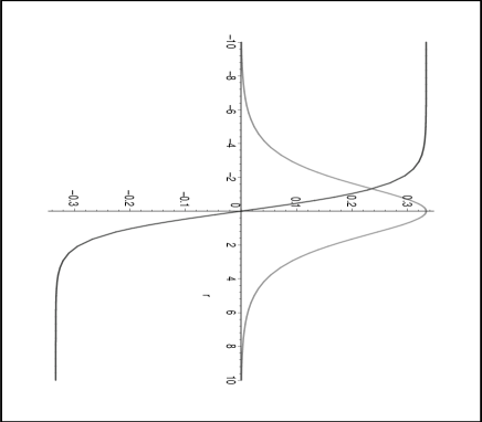
Figure 1: The field $\chi$ is localized inside ($\phi\approx 0$) the $\phi$-domain wall (anti-kink).

III Schroedinger-like equation for the fluctuations

Let us consider linear fluctuations around the solutions ${\phi}$ and ${\chi}$. Consider $\chi=\bar{\chi}+\zeta$ and $\phi=\bar{\Phi}$ where $\zeta$ is the fluctuation of the field $\chi$, $\bar{\Phi}$ and $\bar{\chi}$ are solutions of equations of motion (6) and (7), respectively. Expanding the equations of motion around the fluctuations we find

$$\partial_{\mu}\partial^{\mu}\zeta+\bar{V}_{\chi\chi}\zeta=0.$$ (17)

We consider the following Ansatz for the perturbation around a 3d domain wall extended along the coordinates $(x,y,z)$

$$\zeta=\zeta(r)e^{-i(\omega t-k_{x}x-k_{y}y-k_{z}z)}.$$ (18)

Now substituting this equation into (17) we have

$$-\partial_{r}^{2}\zeta(r)+[-\omega^{2}+k^{2}_{x}+k^{2}_{y}+k^{2}_{z}]\zeta(r)+\bar{V}_{\chi\chi}\zeta(r)=0,$$ (19)

which can be identified with a Schroedinger-like equation. We are interested in solving the quantum mechanics problem to obtain the reflection coefficient of particles as they reach the $\phi$- 3d domain wall of type II. We are only considering elastic collisions and that the particles are hitting the 3d domain wall orthogonally.

Let us consider the Schroedinger potential for the case I, i.e., the 3d domain wall without internal structure. Using equation (5) and the solutions given in (12) we have

$$\bar{V}_{\chi\chi}(r)=4\mu^{2}a^{2}-4\mu^{2}a^{2}(1+\frac{\lambda}{2\mu})\,{\rm sech}^{2}(\lambda ar).$$ (20)

Note that as $\chi=0$ one finds $\phi=\pm a$ (“far” from the wall). In this limit, $\bar{V}_{\chi\chi}(\pm\infty)=4\mu^{2}a^{2}$ is the mass of $\chi$-particles outside the wall, i.e., $m_{\chi}^{2}=4\mu^{2}a^{2}$, where we assume $\chi$ as being the field that describes the particles interacting with the field $\phi$. Thus we have the Schroedinger potential

$$\bar{V}_{\chi\chi}(r)=m_{\chi}^{2}-m_{\chi}^{2}(1+\frac{\lambda}{2\mu})\,{\rm sech}^{2}(\lambda ar).$$ (21)

It is useful to rewrite the righthand side of this equation as $m^{2}_{\chi}+U(r)$, such that we can write (19) as

$$-\partial_{r}^{2}\zeta(r)+[-\omega^{2}+k^{2}_{x}+k^{2}_{y}+k^{2}_{z}+m^{2}_{\chi}]\zeta(r)+U(r)\zeta(r)=0.$$ (22)

Setting $-k^{2}_{r}=-\omega^{2}+k_{x}^{2}+k_{y}^{2}+k_{z}^{2}+m_{\chi}^{2}$ we can write (22) simply as

$$\zeta^{{}^{\prime\prime}}(r)+k^{2}_{r}\zeta(r)-U_{I}(r)\zeta(r)=0,$$ (23)

where $k_{r}$ is the $r$-component of a bulk particle momentum and

$$U_{I}(r)=-m^{2}_{\chi}(1+\frac{\lambda}{2\mu})\,{\rm sech}^{2}(\lambda ar).$$ (24)

Finally let us consider the Schroedinger potential for the case II, i.e., the 3d domain walls with internal structure. Using (5) and the solutions given in (13) we have

$$\bar{V}_{\chi\chi}(r)=4\mu^{2}a^{2}-4\mu^{2}a^{2}(4-\frac{\lambda}{\mu})\,{\rm sech}^{2}(2\mu ar),$$ (25)

with $m_{\chi}^{2}=4\mu^{2}a^{2}$ and

$$\bar{V}_{\chi\chi}(r)=m^{2}_{\chi}-m^{2}_{\chi}(4-\frac{\lambda}{\mu})\,{\rm sech}^{2}(2\mu ar).$$ (26)

Just as in the previous case we have

$$\zeta^{{}^{\prime\prime}}(r)+k^{2}_{r}\zeta(r)-U_{II}(r)\zeta(r)=0,$$ (27)

where the Schroedinger potential now reads

$$U_{II}(r)=-m^{2}_{\chi}(4-\frac{\lambda}{\mu})\,{\rm sech}^{2}(2\mu ar).$$ (28)

We note that in both cases (24) and (28) we have the same $\chi$-particles with squared masses $m_{\chi}^{2}$. However, as $U_{I}$ has width $1/\lambda a$ and depth $-m_{\chi}^{2}(1+\lambda/2\mu)$ whereas $U_{II}$ has width $1/2\mu a$ and depth $-m_{\chi}^{2}(4-\lambda/\mu)$ the $\chi$-mesons clearly should feel different effects.

IV Reflection Probability

The reflection coefficient for potentials like $U(r)=-U_{0}\,{\rm sech}^{2}{\alpha r}$ is given by vilenkin

$$R=\frac{\cos^{2}{\beta}}{\sinh^{2}{\gamma}+\cos^{2}{\beta}}$$ (29)

with $\gamma=\pi k_{r}/\alpha$ and $\beta=(\pi/2)\sqrt{1+4U_{0}/\alpha^{2}}$. Let us now focus on the physics of the case II. Thus for the potential $U_{II}$ we have

$$R=\frac{\cos^{2}{\left(\frac{\pi}{2}\sqrt{17-\frac{4}{N^{2}}}\,\right)}}{\sinh^{2}{\left(\frac{\pi k_{r}\delta}{N^{2}}\right)}+\cos^{2}{\left(\frac{\pi}{2}\sqrt{17-\frac{4}{N^{2}}}\,\right)}}$$ (30)

where we identify $N=\sqrt{\mu/\lambda}$ with the number of $\chi$- 2d domain walls inside the $\phi$- 3d domain walls that have width $\simeq\delta=1/\lambda a$; and $k_{r}=2\pi/\lambda^{\prime}$ is the $r$-component of the wave propagation vector associated with a bulk $\chi$-particle. The estimative about the number $N$ is made by considering the fact that both solutions of type I and II have the same energy $E_{B}^{\phi(I,II)}=(4/3)\lambda a^{3}$, as we mentioned earlier. Note also that the solution of type II can be deformed to the solution of type I by setting $\lambda/\mu=2$. By distributing the whole energy of the $\phi$-3d domain wall of the case II in terms of energy of the internal structures, i.e., $\chi$-domain walls, we have $E_{B}^{\phi(II)}=NE_{B}^{\chi}$, where $E_{B}^{\chi}=(4/3)\lambda a^{3}\sqrt{\lambda/\mu}$ is the energy of a $\chi$-domain wall. This clearly reproduce the value of $N$ aforementioned.

On the one hand, if the wavelength $\lambda^{\prime}$ of the $\chi$-particles is much smaller than the width $\delta$ of the $\phi$-domain wall, thus $k_{r}\gg(\delta^{-1}\!=\!\lambda a)$ and $R$ is exponentially small. On the other hand, if $k_{r}\to 0$, $R\to 1$ and almost all $\chi$-particles are reflected. In Fig. 2 we see $R$ as a function of the number $N$ of $\chi$-domain walls. Note also that for $\lambda/\mu=2$ (domain wall without internal structure) we find $1/N^{2}=2$ and then $R=0$ which implies that there is no reflection.

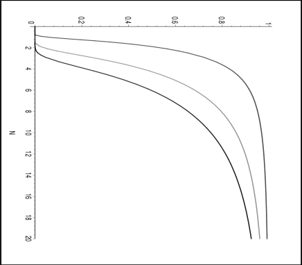
Figure 2: Reflection coefficient $R$ as function of the number of $\chi$-domain walls for a bulk $\chi$-particle colliding with a 3d domain wall with $k_{r}=1,\,5$ and 10 ($\delta=1$).

The behavior of the reflection coefficient can also be seen as a function of the momentum $k_{r}$ of a $\chi$-particle colliding with a $\phi$-3d domain wall fulfilled of $\chi$-domain walls — see Fig. 3.

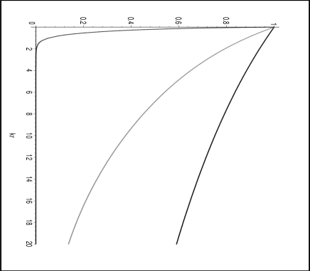
Figure 3: Reflection coefficient $R$ as a function of the momentum $k_{r}$ of a bulk $\chi$-particle colliding with a 3d domain wall with $N=1,\,5$ and 10 $\chi$-domain walls ($\delta=1$).

V Domain Wall Expansion

In this section we investigate how the 3d domain wall expands along its directions as bulk $\chi$-particles collide with it. We use the reflection probability to calculate the rate of momentum transfer of such particles to the domain wall. We can estimate the domain wall acceleration along the transverse coordinate $r$ due to elastic collisions as a function of the reflection coefficient $R$ via transversal force per unit area

$$F_{r}=M_{wall}\,\ddot{r}(t)\simeq\kappa R,$$ (31)

where $r(t)$ is the position (or “radius”) of the domain wall with respect to the origin $O$ into the bulk; $\kappa$ has dependence on the density of colliding bulk particles and their incoming momenta $k_{r}$, that we assume to be time independent.

To relate the size of the coordinates along the domain wall with its position $r(t)$ into the bulk ^[3] we have to make some assumptions. To guide ourselves let us first consider a simple example: a spherical 2d domain wall separating the bulk into two asymmetric regions. The line element on the 2d domain wall depends on $r(t)$ as $ds_{2}^{2}=r(t)^{2}(d\theta^{2}+\sin^{2}{\theta}d\varphi^{2})$; where $(\theta,\varphi)$ are angular coordinates on the surface of the 2d domain wall. In terms of co-moving coordinates we define $\vec{r}(t)=a(t)\vec{r}$ and the line element becomes $ds_{2}^{2}=a(t)^{2}r^{2}(d\theta^{2}+\sin^{2}{\theta}d\varphi^{2})=a(t)^{2}(dx^{2}+dy^{2})$, where $(x,y)$ are co-moving coordinates. The generalization to a 3d domain wall is straightforward: $ds_{3}^{2}=a(t)^{2}(dx^{2}+dy^{2}+dz^{2})$. Another example is considering a domain wall as the boundary of a cone whose size of the domain wall varies with the size of the cone. In our analyze below we consider only the former example.

Until now we have considered a flat 3d domain wall. Indeed, the analysis above is also valid for spherical walls as long as we are considering a regime where the wall radius is very large compared with the wall thickness — thin wall limit. Curved domain walls can be realized in field theory by breaking the $Z_{2}$-symmetry slightly via inclusion of a very small term, e.g., $\epsilon\phi^{3}$, into the original Lagrangian — see kolb . On this account let us consider our 4d universe as a 3d domain wall evolving in time and identify $\vec{r}(t)=a(t)\vec{x}$ with the radius of an expanding 3-sphere whose metric is

$$ds_{4}^{2}=dt^{2}-a(t)^{2}(dx^{2}+dy^{2}+dz^{2}),$$ (32)

where $a(t)$ is the scale factor of our universe and $\vec{x}=(x,y,z)$ are co-moving coordinates.

Now let us consider two important limits. By considering the number of internal structure increases with the time according to the law $N\sim(\beta t)^{\alpha}$ ($\alpha\geq 1$) and substituting into (31) we get to the power-law expansion of an accelerating 3d domain wall

$$a(t)\sim\frac{1}{2}\kappa t^{2},$$ (33)

which is the leading term for large times, i.e., $\beta t\gg k_{r}\delta$. This means an accelerating universe at late time cosmology. This fact agrees with current observations supernovae ; Ries .

Assuming the expansion of our universe, for a brane observer, is driven by an induced scalar field $\varphi$, confined on the 3d domain wall ^[4], depending only on the time coordinate, the $\varphi$ e.o.m and the Friedmann equation are given by

$$\ddot{\varphi}+3H\dot{\varphi}=-\frac{\partial V}{\partial\varphi},$$ (34)

$$3H^{2}\equiv 3\left(\frac{\dot{a}}{a}\right)^{2}=\frac{1}{2}\dot{\varphi}^{2}+V(\varphi).$$ (35)

For exponential potentials as

$$V(\varphi)\sim V_{0}e^{-2\frac{\varphi}{\varphi_{0}}},$$ (36)

which have been much explored in string/M-theory context odintsov ; ac-davis , one can find solutions satisfying (34) and (35):

$$a(t)=a_{0}\left({\beta}{t}\right)^{\frac{1}{2}\varphi_{0}^{2}},\qquad\varphi=\varphi_{0}\ln{\left({\beta}{t}\right)},$$ (37)

where

$$\beta^{-1}=\varphi_{0}\sqrt{\frac{1}{V_{0}}\left(\frac{3}{4}\varphi_{0}^{2}-\frac{1}{2}\right)}.$$ (38)

See, e.g., s.sen for other examples of scalar potentials. Comparing equation (37) with the scale factor $a(t)\sim t^{2}$ given in (33) we find $\varphi_{0}=2$ and $\beta^{-1}=\sqrt{10/V_{0}}$. A necessary requirement for the observed acceleration in the present universe is a power-law expansion $a(t)\sim t^{\alpha}$ with $\alpha>1$.

In the early time cosmology, inflation is a crucial phenomenon for solving several problems such as flatness of universe, monopole problem, etc. At this stage the universe expands according to an exponential-law $a(t)\sim e^{\alpha t}$ ($\alpha>0$). In our scenario for very early times $\beta t\ll k_{r}\delta$ the acceleration is such that the expansion behaves as

$${a}(t)\simeq\frac{1}{2}\kappa\,\beta^{2}t^{2}e^{-\frac{\alpha}{\beta^{2}t^{2}}},$$ (39)

which can be well approximated by an exponential-law $e^{\sqrt{\Lambda_{0}}t}$, for $\alpha=2\pi k_{r}\delta$ small enough (i.e., $k_{r}\delta$ small, that means bulk particles with low momenta $k_{r}$). This inflationary phase starts for $N^{2}>1/2$, i.e., as the number of internal structure becomes to play a fundamental role in the 3d domain wall expansion. This corresponds to the time $t>(1/\beta)(1/\sqrt{2})^{1/\alpha}$. Thus our scenario also reproduces the inflationary phase in the early time universe. The evolution of a dynamical cosmological constant peebles ; steinhardt on the 3d domain wall can be given by the Friedmann equation

$$\left(\frac{\dot{a}}{a}\right)^{2}\simeq\frac{\Lambda(t)}{3},$$ (40)

whose time dependence is $\Lambda(t)\simeq 12(\beta^{2}t^{2}+\alpha)^{2}/t^{6}\beta^{4}$. At early times ($\beta t\ll 1$) the cosmological constant becomes large, $\Lambda_{0}\simeq 12\alpha^{2}/\beta^{4}t^{6}$, and dominant in (40). As time goes larger the cosmological constant approaches to zero according to the power-law $\Lambda\simeq 12/t^{2}$. This goes like the exponent of the exponential factor in (39). For time large enough we should find a transition where the exponential factor is suppressed and the quadratic pre-factor in (39) reproduces the late time cosmology formula (33). If we consider this transition occurring around a time equals to the observed age of our universe, i.e., $t\sim 15$ billion of years we get to the cosmological constant

$$\Lambda\sim 10^{-34}s^{-2}\sim 10^{-119}M_{Pl}^{2}.$$ (41)

Or in terms of 4d Planck length $L_{Pl}=1/M_{Pl}\equiv(8\pi G_{N})^{1/2}$ we define the dimensionless quantity $\Lambda L_{Pl}^{2}\sim 10^{-119}$. According to the analysis above we get to the power-law $\Lambda\sim 1/t^{2}$. Thus we can infer that there is a tendency of having a null cosmological constant in our universe for a very long time. Following the philosophy of dynamical cosmological constant peebles ; steinhardt , or simply quintessence, we could argue that the “observed” cosmological constant assumes the value given in (41) because of the current age of our universe. Although this idea is not new, here it seems to be applicable in a very natural way. This is because the dynamical cosmological constant arises due to the physical effect of bulk particles colliding with a 3d domain wall (our universe), instead arising from a fine-tuned scalar potential — see weinberg ; padna for a review on the cosmological constant problems.

VI Discussions

In early times before inflation we have radiation dominance on the 3d domain wall. The expansion follows according to the power-law $a(t)\sim t^{1/2}$ and temperature decreases as $T\sim a(t)^{-1}$. As temperature decreases, symmetry breaking inside the 3d domain wall provides formation of internal structure favoring momentum transfer of bulk particles to the domain wall. Particles with larger momenta can be mainly reflected only later by a large amount of internal structures on the 3d domain wall while particles with lower momenta can be reflected by just a few number of internal structure and then they can transfer momentum to the domain wall earlier. Thus particles carrying low momenta “ignite” the inflationary expansion in its very beginning. Once this expansion is started the cooling process on the 3d domain wall favors even more the formation of internal structure with the time according to a power-law. At this time, particles with larger momenta also turn to participate of the process. Thus the probability of reflection quickly increases in early times and we find an exponential-law of expansion for our universe represented by the 3d domain wall. This is an inflationary period of our universe, as required by the current cosmology. The acceleration saturates at very late time universe according to a quadratic power-law of expansion. Accelerating universe conforms with current observations. It is a very active subject in the modern cosmology. Several scenarios addressing different problems in accelerating universes such as brane/string gas cosmology and quartessence have recently been considered in the literature — see e.g., brand and ioav , respectively. Our scenario concerning 3d domain walls with internal structures colliding with bulk particles can be considered as a complementary alternative to braneworlds cosmology scenarios dgp ; dg ; defayet ; ac-davis . This “complementarity” may shed some light on issues such as accelerating universes in string/M-theory vijay ; kklt ; kklmmt and the cosmological constant problems weinberg ; padna . A lot of issues concerning our scenario in brane cosmology of warped 5d space-time ac-davis should also be investigated.

- (1) N. Arkani-Hamed, S. Dimopoulos, G.R. Dvali, Phys. Lett. B429, 263 (1998); [arXiv:hep-ph/9803315].
- (2) I. Antoniadis, N. Arkani-Hamed, S. Dimopoulos, G.R. Dvali, Phys. Lett. B436, 257 (1998); [arXiv:hep-ph/9804398].
- (3) L. Randall and R. Sundrum, Phys. Rev. Lett. 83, 3370 (1999); [arXiv:hep-ph/9905221].
- (4) L. Randall and R. Sundrum, Phys. Rev. Lett. 83, 4690 (1999); [arXiv:hep-th/9906064].
- (5) A. Karch and L. Randall, JHEP 0105, 008 (2001); [arXiv:hep-th/0011156].
- (6) P.J.E. Peebles and B. Ratra, Astrophys. J. 325, L17 (1988); B. Ratra and P.J.E. Peebles, Phys. Rev. D37, 3406 (1988); C. Wetterich, Nucl. Phys. B302, 668 (1988).
- (7) R.R. Caldwell, R. Dave and P.J. Steinhardt, Phys. Rev. Lett. 80, 1582 (1998); [arXiv:astro-ph/9708069].
- (8) A.L. Macpherson and B.A. Campbell, Phys. Lett. B347, 205 (1995); [arXiv:hep-ph/9408387].
- (9) J.R. Morris and D. Bazeia, Phys. Rev. D54, 5217 (1996); [arXiv:hep-ph/9607396].
- (10) V. Balasubramanian, Class. Quant. Grav. 21, S1337 (2004); [arXiv:hep-th/0404075].
- (11) S. Kachru, R. Kallosh, A. Linde and S.P. Trivedi, Phys. Rev. D68, 046005 (2003); [arXiv:hep-th/0301240].
- (12) S. Kachru, R. Kallosh, A. Linde, J. Maldacena, L. McAllister and S.P. Trivedi, JCAP 0310, 013 (2003); [arXiv:hep-th/0308055].
- (13) G.W. Gibbons, Supersymmetry, Supergravity and Related Topics, eds. F. de Aguila, J.A. de Azcárraga and L.E. Ibañez (World Scientific, Singapore, 1985). J. Maldacena and C. Nuñez, Int. J. Mod. Phys. A16, 822 (2001); [arXiv:hep-th/0007018].
- (14) P.K. Townsend and M.N.R. Wohlfarth, Phys. Rev. Lett. 91, 061302 (2003); [arXiv:hep-th/0303097].
- (15) N. Ohta, Phys. Rev. Lett. 91, 061303 (2003); [arXiv:hep-th/0303238]. N. Ohta, Prog. Theor. Phys. 110, 269 (2003); [arXiv:hep-th/0304172].
- (16) P.K. Townsend, Cosmic acceleration and M-theory; [arXiv:hep-th/0308149]. E. Teo, A no-go theorem for accelerating cosmologies from M-theory compactifications; [arXiv:hep-th/0412164].
- (17) C.P. Burgess, C. Nuñez, F. Quevedo, G. Tasinato and I. Zavala, JHEP 0308, 056 (2003); [arXiv:hep-th/0305211].
- (18) G. Dvali, G. Gabadadze and M. Porrati, Phys. Lett. B485, 208 (2000); [arXiv:hep-th/0005016].
- (19) G. Dvali and G. Gabadadze, Phys. Rev. D63, 065007 (2001); [arXiv:hep-th/0008054].
- (20) C. Deffayet, Phys. Lett. B502, 199 (2001); [arXiv:hep-th/0010186].
- (21) P. Brax, C. van de Bruck, A.-C. Davis, Rept. Prog. Phys. 67 2183 (2004); [arXiv:hep-th/0404011].
- (22) R. MacKenzie, Nucl. Phys. B303, 149 (1988).
- (23) J.R. Morris, Int. J. Mod. Phys. A13, 1115 (1998); [arXiv:hep-ph/9707519].
- (24) F.A. Brito and D. Bazeia, Phys. Rev. D56, 7869 (1997); [arXiv:hep-th/9706139].
- (25) J.D. Edelstein, M.L. Trobo, F.A. Brito and D. Bazeia, Phys. Rev. D57, 7561 (1998); [arXiv:hep-th/9707016].
- (26) D. Bazeia, H. Boschi-Filho and F.A. Brito, JHEP 9904, 028 (1999); [arXiv:hep-th/9811084].
- (27) D. Bazeia and F.A. Brito, Phys. Rev. D61, 105019 (2000); [arXiv:hep-th/9912015].
- (28) D. Bazeia and F.A. Brito, Phys. Rev. D62, 101701 (2000); [arXiv:hep-th/0005045].
- (29) F.A. Brito and D. Bazeia, Phys. Rev. D64, 065022 (2001); [arXiv:hep-th/0105296].
- (30) E. Witten, Nucl. Phys. B249, 557 (1985).
- (31) P.S. Apostolopoulos and N. Tetradis, Brane cosmological evolution with a general bulk matter configuration, [arXiv:hep-th/0412246].
- (32) P.S. Apostolopoulos, N. Brouzakis, E.N. Saridakis and N. Tetradis, Mirage effects on the brane, [arXiv:hep-th/0502115].
- (33) J.D. Edelstein and J. Mas, JHEP 0406, 015 (2004); [arXiv:hep-th/0403179].
- (34) S. Perlmutter et al., Astrophys. J. 517, 565 (1999); [arXiv:astro-ph/9812133].
- (35) A.G. Riess et al., Astron. J. 116, 1009 (1998); [arXiv:astro-ph/9805201].
- (36) M. Cvetic, Int. J. Mod. Phys. A16, 891 (2001); [arXiv:hep-th/0012105].
- (37) O. DeWolfe, D.Z. Freedman, S.S. Gubser and A. Karch, Phys. Rev. D62, 046008 (2000); [arXiv:hep-th/9909134].
- (38) F.A. Brito, M. Cvetic and S.-C. Yoon, Phys. Rev. D64, 064021 (2001); [arXiv:hep-ph/0105010].
- (39) M. Cvetic and N.D. Lambert, Phys. Lett. B540, 301 (2002), [arXiv:hep-th/0205247].
- (40) D. Bazeia, F.A. Brito and J.R. Nascimento, Phys. Rev. D68, 085007 (2003); [arXiv:hep-th/0306284].
- (41) D. Cremades, L.E. Ibanez and F. Marchesano, Nucl. Phys. B643, 93 (2002); [arXiv:hep-th/0205074]. C. Kokorelis, Nucl. Phys. B677, 115 (2004); [arXiv:hep-th/0207234].
- (42) D. Bazeia, M.J. dos Santos and R.F. Ribeiro, Phys. Lett. A208, 84 (1995); [arXiv:hep-th/0311265].
- (43) D. Bazeia, R.F. Ribeiro and M.M. Santos, Phys. Rev. D54, 1852 (1996).
- (44) D. Bazeia, J.R.S. Nascimento, R.F. Ribeiro and D. Toledo, J. Phys. A30, 8157 (1997); [arXiv:hep-th/9705224].
- (45) M.A. Shifman and M.B. Voloshin, Phys. Rev. D57, 2590 (1998); [arXiv:hep-th/9709137].
- (46) D. Bazeia and A.R. Gomes, JHEP 0405, 012 (2004); [arXiv:hep-th/0403141].
- (47) A. Vilenkin and E.P.S Shellard, Cosmic Strings and other Topological Defects (Cambridge University Press, Cambridge/UK, 1994).
- (48) G. Dvali and S.-H. H. Tye, Phys. Lett. B450, 72 (1999); [arXiv:hep-ph/9812483].
- (49) E.W. Kolb and M.S. Turner, The Early Universe (Addison-Wesley Publishing Company, New York, 1990).
- (50) E. Elizalde, S. Nojiri and S.D. Odintsov, Phys. Rev. D70, 043539 (2004); [arXiv:hep-th/0405034].
- (51) S. Sen and A.A. Sen, Phys. Rev. D63, 124006 (2001); [arXiv:gr-qc/0010092].
- (52) S. Weinberg, The cosmological constant problems, [arXiv:astro-ph/0005265].
- (53) T. Padmanabhan, Phys. Rept. 380, 235 (2003); [arXiv:hep-th/0212290].
- (54) T. Biswas, R. Brandenberger, D.A. Easson and A. Mazumdar, Coupled Inflation and Brane Gases; [arXiv:hep-th/0501194].
- (55) R.R.R. Reis, M. Makler and I. Waga, Class. Quant. Grav. 22, 353 (2005); [arXiv:astro-ph/0501613].