CERN–PH–TH/2005–19

Scalar perturbations in regular two-component bouncing cosmologies

V. Bozza^a,b,c and G. Veneziano^d,e

^a Centro studi e ricerche “Enrico Fermi”, via Panisperna 89/A, Rome, Italy.
^b Dipartimento di Fisica “E. R. Caianiello”, Università di Salerno, I-84081 Baronissi, Italy.
^c Istituto Nazionale di Fisica Nucleare, Sezione di Napoli, Naples, Italy.
^d CERN, PH Dept., TH Unit, CH-1211, Geneva 23, Switzerland.
^e Collège de France, 11 place Marcelin-Berthelot, 75005 Paris, France.

We consider a two-component regular cosmology bouncing from contraction to expansion, where, in order to include both scalar fields and perfect fluids as particular cases, the dominant component is allowed to have an intrinsic isocurvature mode. We show that the spectrum of the growing mode of the Bardeen potential in the pre-bounce is never transferred to the dominant mode of the post-bounce. The latter acquires at most a dominant isocurvature component, depending on the relative properties of the two fluids. Our results imply that several claims in the literature need substantial revision.

PACS: 98.80.-k, 98.65.Dx, 98.80.Es, 11.25.Wx

Bouncing cosmologies have been proposed as possible alternatives to standard inflation in string-inspired (e.g. Pre-Big Bang [1], ekpyrotic/cyclic [2]) scenarios. In order to compare the predictions of these scenarios with observations, it is crucial to follow the evolution of cosmological perturbations from the initial vacuum-normalized state, through the bounce, all the way until decoupling. Nevertheless, there is no general agreement on the true influence of a bounce on cosmological perturbations. In particular, it is not clear whether the Pre-Bounce growing mode of the Bardeen potential leaves any trace in the Post-Bounce, or whether it just completely matches a decaying mode [3]. Only in the former case can the claim that the ekpyrotic/cyclic scenario is in agreement with CMB data be defended.

Studies of specific regular models apparently led to different results, suggesting that both possibilities can arise, depending on the specific model one assumes for the regular bounce. In spatially closed universes, a regular bounce from contraction to expansion can be triggered by the spatial curvature term in the Friedman equations [4]. In this case, the transfer matrix relating Post-Bounce modes to Pre-Bounce perturbations depends on the momentum scale $k$, suggesting that non-trivial matching conditions hold. These models have the advantage of being completely embedded into General Relativity, but they need fine-tuning in the initial conditions in order to have a sufficiently long collapse.

Alternatively, one can start from a spatially flat universe, avoiding the complications of spatial curvature. However, Friedman equations imply that a bounce from contraction to expansion necessarily violates the null energy condition (NEC). This violation can be induced by high energy and high curvature corrections to General Relativity or can be directly introduced by a ghost field dominating during the bounce. In this class of models, contradictory results have emerged up to now. Peter & Pinto-Neto [5] and Finelli [6] find some mixing between the growing and decay modes of the Bardeen potential, while Gasperini, Giovannini & Veneziano [7], Cartier [8], and Allen & Wands [9] find that the growing mode of the Bardeen potential in the Pre-Bounce exactly matches the decaying mode in the Post-Bounce.

In this letter we report the results of the study of a wide class of regular bouncing cosmological models, containing, as particular cases, all the above-mentioned two-source regular models. We confirm that the Pre-Bounce Bardeen growing mode matches the Post-Bounce decaying mode. The only possible mode mixing is between the two components that are present in the cosmological description, as a consequence of the normal interplay between adiabatic and isocurvature perturbations. We present hereafter the key arguments and give the main results, postponing most details to a later publication [10].

We consider a two-component cosmology, where the first component dominates at early and late times, while the secondary one has negative energy density and triggers the bounce from contraction to expansion in a fully regular fashion. It is well known that ghosts or negative energy density fluids induce instabilities at a quantum level, but this has nothing to do with the evolution of classical perturbations, which is completely under control, as we shall explicitly show. One may regard the secondary field as an effective term in our 4-dimensional Friedman equations simulating corrections from high energy, high curvature, extra-dimensions, finite string size, or whatever else one can imagine. One can then look at the regular bounce obtained in such an effective description at a classical level using the paradigm of General Relativity, without worrying about quantum instabilities which should be properly addressed only within a yet unavailable complete theory of the bounce. These considerations confer a huge interest to ghost-induced-bounces as the only effective models of spatially-flat bouncing cosmologies which can be investigated within the frame and with the instruments of General Relativity. In some sense, they are the only models worth speaking about at the effective level!

The background equations are

$$3\mathcal{H}^{2}=a^{2}\rho$$ (1)

$$\mathcal{H}^{2}+2\mathcal{H}^{\prime}=-a^{2}p$$ (2)

$$\rho^{\prime}+3\mathcal{H}(\rho+p)=0,$$ (3)

where a prime denotes derivative w.r.t. conformal time $\eta$, $a$ is the scale factor, $\mathcal{H}=a^{\prime}/a$, and we have set $8\pi G=1$. The total energy density is $\rho=\rho_{a}+\rho_{b}$ and the pressure is $p=p_{a}+p_{b}$. The two fluids satisfy the continuity equation (3) independently, i.e. we assume no interaction between the two fluids other than gravitational. We shall set $\eta=0$ at the bounce, i.e. when $\mathcal{H}$ changes sign. A typical background solution starts from a contraction driven by the first fluid, which ends when the secondary fluid’s density becomes of the same order as that of the first fluid. We will call this time $-\eta_{b}$ and normalize $\eta$ in such a way that $\eta_{b}\simeq 1$. As we are restricting ourselves to spatially-flat cosmologies, the null energy condition (NEC, hereafter) is necessarily violated, i.e. $\rho+p$ must change sign at some time $\eta_{\mathrm{NEC}}$, with $-1<\eta_{\mathrm{NEC}}<0$. After the bounce the NEC is restored, the secondary fluid becomes subdominant again, and an expansion phase dominated by the first fluid follows.

We shall consider only scalar perturbations, since these are both the most relevant and the most controversial. The perturbed line element takes the well-known form

$$ds^{2}= a^{2}(\eta)\left\{(1+2\phi)d\eta^{2}-2B_{,i}d\eta dx^{i}\right.$$ (4)

$$\left.-\left[(1-2\psi)\delta_{ij}+2E_{,ij}\right]dx^{i}dx^{j}\right\},$$

while the perturbed energy–momentum tensor of the first source reads:

$${{(T_{a})}^{\mu}}_{\nu}=\left(\begin{array}[]{cc}\rho_{a}+\delta\rho_{a}&-(\rho_{a}+p_{a})\mathcal{V}_{a,i}\\ (\rho_{a}+p_{a})\mathcal{V}_{a,i}&-(p_{a}+\delta p_{a})\delta_{ij}\\ \end{array}\right),$$ (5)

where $\mathcal{V}_{a}$ is its velocity potential. The same expression holds for the secondary fluid, the subscript $a$ being replaced by $b$.

In order to keep our treatment as general as possible, we introduce the following gauge-invariant relations among the perturbations of the sources:

$$\!\!\!\!\delta p_{a}=c_{a}^{2}\delta\rho_{a}+\alpha(\rho_{a}+p_{a})\mathcal{V}_{a};\;\;\alpha=\frac{p_{a}^{\prime}-c_{a}^{2}\rho_{a}^{\prime}}{\rho_{a}+p_{a}};\;\;\delta p_{b}=c_{b}^{2}\delta\rho_{b}.$$ (6)

Notice that if $c_{a}^{2}\neq p_{a}^{\prime}/\rho_{a}^{\prime}$, the additional dependence on the velocity potential generates an isocurvature mode

$$\tau_{a}\delta S_{a}=\delta p_{a}-(p_{a}^{\prime}/\rho_{a}^{\prime})\delta\rho_{a}=\alpha(\rho_{a}+p_{a})\left(\mathcal{V}_{a}-\delta\rho_{a}/\rho_{a}^{\prime}\right).$$ (7)

It is a trivial exercise to prove that a scalar field $\varphi$ with a self-interaction potential $V(\varphi)$ satisfies these relations with $c_{a}^{2}=1$ and $\alpha=-2a^{2}V_{,\varphi}/\varphi^{\prime}$. Therefore, these relations include perfect fluids and scalar fields as particular cases of a general class of sources and ensure a wide generality to our treatment. Allen & Wands’ model [9] is recovered with the scalar field choice for the first fluid and $c_{b}^{2}=1$. The perfect-fluid model studied by Finelli [6] is recovered setting $\alpha=0$, $c_{b}^{2}=2c_{a}^{2}+1/3$. The model by Peter & Pinto-Neto [5] corresponds to $\alpha=0$, $c_{a}^{2}=1/3$, $c_{b}^{2}=1$. The generalization to the case where an intrinsic isocurvature mode for the secondary fluid is present poses no major difficulties, but will not be considered here for simplicity.

The first subtlety in the study of perturbations in cosmological bounces is the choice of a gauge where all variables stay finite and small enough for the linear theory to apply. In particular, we have to be sure that the perturbative variables we are considering will not diverge at any point. From the physical point of view the requirement is that all components of the metric and of the energy–momentum tensor stay finite at least in one convenient gauge. If we assume that such a gauge exists (if it does not then the model under consideration cannot be a stable solution of Einstein equations), we deduce that $\phi$, $\psi$, $B$, $E$, $\delta\rho_{i}$, $\delta p_{i}$ and $(\rho_{i}+p_{i})\mathcal{V}_{i}$ stay finite and small in that gauge. We will refer to it as the regular gauge. Note that the total velocity potential $\mathcal{V}$ is allowed to diverge in the regular gauge at $\eta=\eta_{\mathrm{NEC}}$ when $\rho+p=0$ (NEC violation), since what matters is that the energy–momentum tensor components stay finite. Our attitude will be just to assume that such a regular gauge exists and to build gauge-invariant quantities out of perturbations in this gauge.

The Bardeen potential $\Psi=\psi+\mathcal{H}(E^{\prime}-B)$ is indeed a first regular combination. The widely used $\zeta=\psi+\mathcal{H}\mathcal{V}$ may diverge at $\eta_{\mathrm{NEC}}$. However, we can replace it by

$$\tilde{\zeta}=(\mathcal{H}^{2}-\mathcal{H}^{\prime})(\psi+\mathcal{H}\mathcal{V}),$$ (8)

which is guaranteed to be regular, since $2(\mathcal{H}^{2}-\mathcal{H}^{\prime})\mathcal{V}=a^{2}(\rho+p)\mathcal{V}$ is finite in the regular gauge. We then introduce individual gauge-invariant variables

$$\tilde{\zeta}_{a}=\frac{1}{2}a^{2}(\rho_{a}+p_{a})(\psi+\mathcal{H}\mathcal{V}_{a})$$ (9)

$$\Psi_{a}=\frac{1}{2}a^{2}(\rho_{a}^{\prime}\psi+\mathcal{H}\delta\rho_{a}),$$ (10)

and similarly for the $b$ fluid. All these variables are regular by construction. From the definition of $\tilde{\zeta}$ and the 00 component of the Einstein equations, we have

$$\tilde{\zeta}=\tilde{\zeta}_{a}+\tilde{\zeta}_{b};\;\;\;\;(3\tilde{\zeta}+k^{2}\Psi)\mathcal{H}+\Psi_{a}+\Psi_{b}=0.$$ (11)

The perturbations of the continuity equations of each fluid can be combined to give coupled second order equations for $\tilde{\zeta}_{a}$ and $\tilde{\zeta}_{b}$. Introducing the canonical (Sasaki–Mukhanov) variables [11] $v_{a}=\tilde{\zeta}_{a}/[c_{a}(\rho_{a}+p_{a})^{1/2}\mathcal{H}]$ and $v_{b}=\tilde{\zeta}_{b}/[c_{b}(\rho_{b}+p_{b})^{1/2}\mathcal{H}]$, we find

$$v_{a}^{\prime\prime}+\left(c_{a}^{2}k^{2}-z_{a}^{\prime\prime}/z_{a}\right)v_{a}=O(\rho_{b}/\rho_{a})^{1/2}$$ (12)

$$v_{b}^{\prime\prime}+\left(c_{b}^{2}k^{2}-z_{b}^{\prime\prime}/z_{b}\right)v_{b}=O(\rho_{b}/\rho_{a})^{1/2},$$ (13)

with $z_{a}=a^{2}(\rho_{a}+p_{a})^{1/2}/(c_{a}\mathcal{H})$ and $z_{b}=a^{(1+3c_{b}^{2})}(\rho_{b}+p_{b})^{1/2}/c_{b}$. These equations also identify $c_{a}^{2}$ and $c_{b}^{2}$ as the correct definitions of the sound speed for the two components.

These equations decouple only in the limit $\rho_{b}/\rho_{a}\rightarrow 0$. Both Mukhanov variables are normalized to vacuum fluctuations and thus are of order $1/\sqrt{2k}$ in the asymptotic past. However, we have $\tilde{\zeta}_{b}=\sqrt{(\rho_{b}+p_{b})/(\rho_{a}+p_{a})}\tilde{\zeta}_{a}$ and a hierarchy can therefore be established between these two variables in this limit. In this sense, the $O(\rho_{b}/\rho_{a})^{1/2}$ contains all terms that are irrelevant in the asymptotic past, including couplings between the two variables.

Although it is not necessary, let us assume for simplicity that the Pre-Bounce can be described by a power law $a(\eta)\simeq(-\eta)^{q}$. Defining $\Gamma=\frac{p^{\prime}}{\rho^{\prime}}$, the following general relations are implied by the background equations

$$q=\frac{2}{1+3\Gamma},\;\;\alpha\sim\frac{q(1+3c_{a}^{2})-2}{-\eta}.$$ (14)

If $\alpha=0$, we get $\Gamma=c_{a}^{2}$, which is the case of a perfect fluid. A well-known case of a source where $\alpha$ contributes to the background is the case of a scalar field with an exponential potential $e^{-\lambda\varphi}$. Then $c_{a}^{2}=1$, but $\Gamma$ can assume any value depending on $\lambda$. This case is discussed in Ref. [9]. A stiffer $\eta$-dependence for $\alpha$ would make it rapidly subdominant, while a softer one would render the vacuum normalization problematic and will not be considered.

The secondary field evolves according to its continuity equation $\rho_{b}\sim(-\eta)^{-3q(1+c_{b}^{2})}$. Exploiting the fact that the two fluids have comparable densities at time $\eta=-1$, at earlier times we find $\rho_{b}/\rho_{a}\simeq(-\eta)^{-q(1+3c_{b}^{2})+2}$.

In the power law regime, Eqs. (12) and (13) give

$$v_{a}= \sqrt{|\eta|}C_{a}H^{(1)}_{\nu_{a}}(c_{a}\sqrt{k}|\eta|)$$ (15)

$$v_{b}= \sqrt{|\eta|}C_{b}H^{(1)}_{\nu_{b}}(c_{b}\sqrt{k}|\eta|).$$ (16)

with $\nu_{a}=\frac{1}{2}-q$, $\nu_{b}=\frac{1}{2}(3c_{b}^{2}q-1-q)$ and $H_{\nu}^{(1)}$ is the Hankel function of the first kind; $C_{a}$ and $C_{b}$ are pure numbers of order 1. The initial conditions for $\tilde{\zeta}_{a}$, $\tilde{\zeta}_{b}$, $\Psi_{a}$ and $\Psi_{b}$ can be derived from those we just imposed on Mukhanov’s variables.

From the perturbations of the continuity equations, it is straightforward to write a set of first-order differential equations for $\tilde{\zeta}$, $\Psi$, $\tilde{\zeta}_{b}$ $\Psi_{b}$. However, it is more useful for our purposes to write these equations in their integral form

$$\!\!\!\!\!\!\!\!\Psi \!\!\!\!=\frac{\mathcal{H}}{a^{2}}\left[\frac{c_{1}(k)}{k^{2}}+\int\frac{a^{2}}{\mathcal{H}^{2}}\tilde{\zeta}d\eta\right]$$ (20)

$$\!\!\!\!\!\!\!\!\tilde{\zeta} \!\!\!\!=a^{2}(\rho_{a}+p_{a})\left[c_{2}(k)-\int\frac{c_{a}^{2}\mathcal{H}}{a^{2}(\rho_{a}+p_{a})}k^{2}\Psi d\eta\right.$$

$$\left.-\int\frac{\alpha}{a^{2}(\rho_{a}+p_{a})}\tilde{\zeta}_{b}d\eta+\int\frac{c_{b}^{2}-c_{a}^{2}}{a^{2}(\rho_{a}+p_{a})}\Psi_{b}d\eta\right]$$

$$\!\!\!\!\!\!\!\!\Psi_{b} \!\!\!\!=\frac{\mathcal{H}}{a^{1+3c_{b}^{2}}}\left[c_{3}(k)-\int\frac{a^{1+3c_{b}^{2}}k^{2}}{\mathcal{H}}\tilde{\zeta}_{b}d\eta\right.$$

$$\left.+\int\frac{a^{3+3c_{b}^{2}}(\rho_{b}+p_{b})}{2\mathcal{H}}k^{2}\Psi d\eta\right]$$

$$\!\!\!\!\!\!\!\!\tilde{\zeta}_{b} \!\!\!\!=a^{1+3c_{b}^{2}}\mathcal{H}(\rho_{b}+p_{b})\left[c_{4}(k)+\int\frac{c_{b}^{2}}{a^{1+3c_{b}^{2}}\mathcal{H}(\rho_{b}+p_{b})}\Psi_{b}d\eta\right.$$

$$\left.+\int\frac{a^{1-3c_{b}^{2}}}{2\mathcal{H}^{2}}\tilde{\zeta}d\eta\right]\,,$$

Now we are ready to analyse the evolution of the modes that are well outside the horizon at the bounce ($k\ll 1$). The discussion can be made in terms of the two parameters $\Gamma$ and $c_{b}^{2}$, which express the background evolution of the two fluids. Not all values of these two parameters are relevant to bouncing cosmologies. Indeed, as a first constraint, the condition that $\rho_{b}/\rho_{a}$ must grow during contraction (otherwise there is no bounce), excludes the half-plane $c_{b}^{2}<\Gamma$. A correct vacuum normalization requires $c_{a}^{2},c_{b}^{2}>0$. Finally, we require $\Gamma>-1/3$, in order to discard superinflationary backgrounds. For the sake of generality we do not impose the causality constraint $c_{a}^{2},c_{b}^{2}\leq 1$. In Fig. 1, we show the allowed regions in the cases $\alpha\neq 0$ and $\alpha=0$, the forbidden ones being shaded.

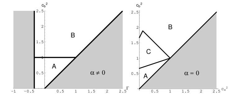
Figure 1: The parameter space in the general case (left) and in the perfect fluid case (right).

The four constants $c_{i}(k)$ can be determined by matching them to the long-wavelength limit of Eqs. (15),(16):

$$c_{1}(k)\sim k^{\nu_{a}},\;c_{2}(k)\sim k^{-\nu_{a}},\;c_{3}(k)\sim k^{-\nu_{b}},\;c_{4}(k)\sim k^{\nu_{b}}.$$ (21)

Now we have to compute the evolution of the individual terms in Eqs. (20)–(20) and find the dominant contribution at horizon re-entry after the bounce. We will discard any numerical factors of order 1, just keeping the dependences on $k$ and $\eta$, the only dimensional parameters in our analysis. In these equations, each variable is expressed as the sum of a “homogeneous” mode and several integrals, one for each coupling term. The homogeneous mode of each variable persists through the bounce and after the bounce, and thus poses no difficulty. To evaluate the integrals, we note that, far from the bounce, we can replace all the functions by their asymptotic power law behaviours . Thus each integrand $f(\eta)$ assumes the generic form $c_{i}(k)|\eta|^{s}$ and, for each integral, we generically have, in the Pre-Bounce:

$$\int\limits^{\eta}c_{i}(k)|\eta|^{s}d\eta\sim c_{i}(k)|\eta|^{s+1},\;\;\;\eta<-1,$$ (22)

where the integration constant is set to zero in order to match, in the far past, the asymptotic solutions implied by (15), (16).

To evaluate the integrals in the Post-Bounce, we can split the integration domain in three intervals, covering the full Pre-Bounce, the Bounce and the Post-Bounce separately. We have

$$\int\limits^{-1}c_{i}(k)|\eta|^{s}d\eta\sim c_{i}(k),\;\;\int\limits_{-1}^{1}f(\eta)d\eta\sim c_{i}(k),$$

$$\int\limits_{1}^{\eta}c_{i}(k)|\eta|^{s}d\eta\sim c_{i}(k)\left[1-\eta^{s+1}\right].$$ (23)

The first integral is just Eq. (22) evaluated at $\eta=-1$, while the third is evaluated using the power-law expansion for the integrand $f(\eta)$ in the Post-Bounce. More subtle is the bounce contribution. Since all the curvature and time scales are fixed by the time normalization choice $\eta_{b}=1$, the only scales that can be introduced by this contribution are $k$ and $\eta$. Yet, the integrand is a combination of $k$-independent backgrounds, and integration over the finite bounce interval eliminates $\eta$ from the final result. Hence the bounce contribution is of the same order as $c_{i}(k)$. An apparent complication comes from the divergence of some integrands in Eqs. (20)–(20) at the bounce. Of course, these divergences do not affect the regularity of the gauge-invariant variables, since all the integrals are multiplied by proper factors, which compensate these divergences. Mathematically we can further split the bounce integrals in two pieces, before and after $\eta=0$. The limiting value of the gauge-invariant variable at $0^{-}$ fixes the initial condition for the second integral starting from $0^{+}$ (recall that our integral equations are just another representation of differential equations, which admit a regular expansion for the solution at $\eta=0$). Afterwards, the dimensional argument can be applied safely.

At late times ($\eta\gg 1$) the dominant term depends on the value of $s$

$$\int\limits^{\eta}f(\eta)d\eta\sim\left\{\begin{array}[]{ll}c_{i}(k),&s<-1\\ c_{i}(k)\eta^{s+1},&s>-1.\end{array}\right.$$ (24)

Calculating all the integrals recursively, we can build a $k$-expansion for each of the four independent modes $c_{i}(k)$. Evaluating the solutions in this way obtained at the horizon re-entry $\eta\sim 1/k$, we can pick out the dominant contributions and read their spectra.

Let us first discuss the general case where $\alpha$ is different from zero. This includes bounces with tracking scalar fields and all asymmetric bounces. We can distinguish two regions in the plane ($\Gamma$,$c_{b}^{2}$), illustrated in the left panel of Fig. 1. In region A (defined by $c_{b}^{2}<1$), $\Psi$ and $\tilde{\zeta}$ develop a typical adiabatic spectrum, determined by the dominant fluid. We have $\Psi^{A}\sim\tilde{\zeta}^{A}\sim c_{1}(k)$. In region B, covering the rest of the plane, $\Psi$ and $\tilde{\zeta}$ acquire the spectrum of the secondary component, so that $\Psi^{B}\sim\tilde{\zeta}^{B}\sim c_{3}(k)$. The individual variables $\tilde{\zeta}_{a}$ and $\tilde{\zeta}_{b}$ follow the behaviour of $\tilde{\zeta}$. Notice that on the border line ($c_{b}^{2}=1$), the two spectra coincide. It was this line that was explored in Ref. [9]. In the particular case $\alpha=0$, we have $\Gamma=c_{a}^{2}$ and the bounce is always perfectly symmetric. This includes bounces with two perfect fluids or scalar fields dominated by their kinetic energy (compare Refs. [6, 5]). The time-reversal symmetry induces several cancellations in the integrals, allowing the creation of an intermediate region C, defined by $(2+c_{a}^{2})/3<c_{b}^{2}<min(5/3+2c_{a}^{2},2-c_{a}^{2})$. In this region, $\tilde{\zeta}_{a}$ and $\tilde{\zeta}_{b}$ keep their original spectrum, without mixing. Nevertheless, $\Psi$ and $\tilde{\zeta}$ are dominated by the first component, so that $\Psi^{C}\sim\tilde{\zeta}^{C}\sim c_{1}(k)$. Finally, in region B, $\Psi$ and $\tilde{\zeta}$ get an extra $k^{2}$ factor w.r.t. the case $\alpha\neq 0$.

In no case does the spectrum $k^{-2}c_{1}(k)\sim k^{-\frac{3}{2}-q}$ of the Pre-Bounce growing mode of $\Psi$ survive at the Post-Bounce horizon re-entry. All the above results have been confirmed by numerical integration of the equations [10]. Our results support the conclusion that a smooth bounce cannot generate a scale-invariant spectrum via the mode-mixing mechanism advocated in [2]. One can argue, of course, that the way string theory will actually describe the bounce has no resemblance to a regular bounce described by General Relativity. In that case, understanding the spectrum of perturbations in such models will have to wait until a full stringy treatment of the problem is found. On the other hand, claims that such a treatment will automatically lead to a flat spectrum through mode-mixing appear unjustified.

Some authors, working within specific models, have reached conclusions that appear to contradict our general analysis. In Ref. [5], Eq. (26) provides an analytical solution $f(\eta)=\eta/(1+\eta^{2})^{2}$ for perturbations outside the horizon which is valid both far from and through the bounce. However, the authors use an approximate form ($f_{app}(\eta)=1/\eta^{3}$) of this solution far from the bounce and then match $f_{app}$ to $f$ just before the bounce. Had they used $f$ from the beginning throughout the bounce, they would have found no mixing. No surprise, therefore, that the mixing they find is at order $\eta^{-5}$, which is just the next to leading order term in $f(\eta)$, which is missing in $f_{app}(\eta)$. Had they kept the $\eta^{-5}$ term in $f_{app}(\eta)$ they would have found mixing at the order $\eta^{-7}$. We thus conclude that the mixing they find is just an artifact of their matching procedure.

In the case of Ref. [6], the limit $\gamma\rightarrow 0$ ($k\rightarrow 0$ in our notation), used to evaluate the final spectrum, just selects the infrared modes at the bounce. However, the final spectrum should be evaluated at the horizon re-entry, after the decaying mode has gone away; it would correspond to $\gamma\rightarrow 0$ while keeping $\gamma z$ (our $k\eta$) of order 1. Finally, a recent paper [12] studying the slow contraction of the ekpyrotic model in the synchronous gauge agrees with our general conclusions. However, these authors ignore a possible divergence of the $\zeta$ variable at the NEC-violation point, and this appears to restrict significantly the applicability of their argument.

V.B. thanks the CERN Theory Unit for hospitality. We acknowledge useful discussions with F. Finelli, J. Hwang, V. Mukhanov, P. Peter and D. Schwarz.

References

- [1] G. Veneziano, Phys. Lett. B 265, 287 (1991); M. Gasperini and G. Veneziano, Astropart. Phys. 1, 317 (1993); R. Brustein, M. Gasperini, M. Giovannini, V. Mukhanov, and G. Veneziano, Phys. Rev. D 51, 6744 (1995); M. Gasperini and G. Veneziano, Phys. Rep. 373, 1 (2003).
- [2] J. Khouri, B. A. Ovrut, P. J. Steinhardt, and N. Turok, Phys. Rev. D 66, 046005 (2002); S. Gratton, J. Khoury, P. J. Steinhardt, and N. Turok, Phys. Rev. D 69, 103505 (2004); A. J. Tolley, N. Turok, and P. J. Steinhardt, Phys. Rev. D 69, 106005 (2004).
- [3] R. Brandenberger and F. Finelli, JHEP 0111, 056 (2001); J. Hwang, Phys. Rev. D 65, 063514 (2002); J. Hwang and H. Noh, Phys. Lett. B 545, 207 (2002); J. Martin, P. Peter, N. Pinto-Neto, and D.J. Schwarz, Phys. Rev. D 65, 123513 (2002); R. Durrer and F. Vernizzi, Phys. Rev. D 66, 083503 (2002).
- [4] J. Hwang and H. Noh Phys. Rev. D 65, 124010 (2002); C. Gordon and N. Turok Phys. Rev. D 67, 123508 (2003); J. Martin and P. Peter Phys. Rev. D 68, 103517 (2003); J. Martin and P. Peter Phys. Rev. Lett. 92, 061301 (2004).
- [5] P. Peter and N. Pinto-Neto, Phys. Rev. D 66, 063509 (2002).
- [6] F. Finelli, JCAP 0310, 011 (2003).
- [7] M. Gasperini, M. Giovannini, and G. Veneziano, Phys. Lett. B 569, 113 (2003); Nucl. Phys. B 694, 206 (2004).
- [8] C. Cartier, hep-th/0401036.
- [9] L. Allen and D. Wands, Phys. Rev. D 70, 063515 (2004).
- [10] V. Bozza and G. Veneziano, in preparation.
- [11] V.F. Mukhanov, H.A. Feldman, and R.H. Brandenberger, Phys. Rep., 215, 203 (1992).
- [12] P. Creminelli, A. Nicolis, and M. Zaldarriaga, hep-th/0411270.