[

Deconfinement Phase Transition in a 3D Nonlocal U(1) Lattice Gauge Theory

Abstract

We introduce a 3D compact U(1) lattice gauge theory having nonlocal interactions in the temporal direction, and study its phase structure. The model is relevant for the compact QED₃ and strongly correlated electron systems like the t-J model of cuprates. For a power-law decaying long-range interaction, which simulates the effect of gapless matter fields, a second-order phase transition takes place separating the confinement and deconfinement phases. For an exponentially decaying inter- action simulating matter fields with gaps, the system exhibits no signals of a second-order transition.

DOI: 10.1103/PhysRevLett.94.211601                   PACS numbers: 11.15.Ha, 12.38.Gc, 71.27.+a

]

The U(1) lattice gauge theory (LGT) in three dimensions (3D) coupled to matter fields describes various interesting physical systems. The compact QED₃ is just a such system and its phase structure has been studied by various methods[1]. In condensed matter physics, interesting observations were made that the strongly-correlated electron systems in two dimensions like the antiferromagnetic Heisenberg spin model, the t-J model of high-$T_{c}$ cuprates, and the fractional quantum Hall states are described by 3D U(1) gauge theories due to the introduction of auxiliary collective fields[2, 3, 4, 5].

For the case without matter-field couplings, Polyakov [6] showed that the 3D compact U(1) gauge theory is always in the confinement phase due to the monopole (instanton) condensation. For the case with couplings to matter fields, there is still no consensus on the question of whether the system in two spatial dimensions exhibits a phase transition into a deconfinement phase. Probably the answer depends on the properties of coupled matter fields. This question is important because the “fractionalization” of electrons may be interpreted as the deconfinement phenomenon of U(1) gauge dynamics. For the t-J model, the possibility of charge-spin separation (CSS) is of great interest since it may explain various anormalous behaviors of the metallic state of cuprates[7]. In Ref.[8] it was argued that the CSS takes place below certain critical temperature $(T)$ as a deconfinement (perturbative) phase of an effective U(1) LGT which is derived by the hopping expansion of spinons and holons in the slave-particle representation at finite $T$. In related works, Nagaosa[9] argued that the deconfinement phase is possible above some $T$, whereas Nayak[10] argued that deconfinement does not occur at any $T$. The deconfinement phase at $T=0$ for systems with gapless excitations are supported in Ref.[11] and denied in Ref.[12].

In this Letter, we introduce and study a LGT with nonlocal interactions in order to investigate the phase structure of compact U(1) gauge theories coupled to matter fields on the 3D lattice (2D system at $T=0$). We first consider the cases of massless and massive relativisitic matter fields. Then we apply the model to the nonrelativistic electron systems. The results of this paper for gapless excitations in electron systems shall complement our previous result of CSS[8] because the hopping expansion employed there may be inadequate for massless excitations at $T=0$.

Let us start with the path-integral representation of the partition funciton $Z$ of gauge field $U_{x\mu}$ and (bosonic and/or fermionic) matter fields $\phi_{x}$,

$$Z = \int\prod_{x}d\bar{\phi}_{x}d\phi_{x}\prod_{x,\mu}dU_{x\mu}\exp(A),$$ (1)

$$A = -\sum_{x,y}\bar{\phi}_{x}\Gamma_{xy}(U)\phi_{y}+A_{U},$$ (2)

$$A_{U} = q\sum_{x,\mu<\nu}(\bar{U}_{x\nu}\bar{U}_{x+\hat{\nu},\mu}U_{x+\hat{\mu},\nu}U_{x\mu}+c.c.),$$ (3)

where $x=(x_{0},x_{1},x_{2})$ is the site-index of the 3D lattice of the size $V=N_{0}N_{1}N_{2}$ with the periodic boundary condition, $\mu(=0,1,2)$ is the (imaginary) time and spatial direction index, $\phi_{x}$ is the matter field on $x$, $U_{x\mu}=\exp(i\theta_{x\mu})\;(-\pi<\theta_{x\mu}\leq\pi)$ is the $U(1)$ gauge variable on the link $(x,x+\hat{\mu})$, $\Gamma_{xy}(U)$ represents the local couplings of $\phi_{x}$ to $U_{x\mu}$.

By integrating over $\phi_{x}$, we obtain an effective gauge theory,

$$Z = \int\prod_{x,\mu}dU_{x\mu}\exp\Big{[}f\;{\rm Tr}\;\log\;\Gamma_{xy}(U)+A_{U}\Big{]},$$ (4)

where $f$ is a parameter counting the statistics and internal degrees of freedom of $\phi_{x}$. Due to the $({\rm Tr}\;\log)$ term, the effective gauge theory becomes nonlocal. For relativistic matter fields, it is expanded as a sum over all the closed random walks ${\cal R}$ (loops including backtrackings) on the 3D lattice which represent world lines of particles and antiparticles as

$${\rm Tr}\;\log\;\Gamma_{xy}(U)=\sum_{\cal R}\frac{\gamma^{L[{\cal R}]}}{L[{\cal R}]}\prod_{(x\mu)\in{\cal R}}U_{x\mu}.$$ (5)

$L[{\cal R}]$ is the length of ${\cal R}$, and $\gamma=(6+m^{2})^{-1}$ is the hopping parameter (6 is the number of links emanating from each site, and $m$ is the mass of the matter field in unit of the lattice spacing). For the constant gauge-field configuration $U_{x\mu}=1$, the expansion in (5) is logarithmically divergent $\sim\log m$ as $m\rightarrow 0$ due to the lowest-energy zero-momentum mode.

Below we shall study a slightly more tractable model than that given by Eq.(4). It is suggested from the formal hopping expansion (5), and obtained by retaining only the rectangular loops extending in the temporal direction in the loop sum and choosing their coefficients optimally as follows;

$$Z_{\cal T} = \int\prod_{x,\mu}dU_{x\mu}\exp(A_{\cal T}),$$ (6)

$$A_{\cal T} = g\sum_{x}\sum_{i=1}^{2}\sum_{\tau=1}^{N_{0}}c_{\tau}(V_{x,i,\tau}+\bar{V}_{x,i,\tau})+A_{S},$$ (7)

$$V_{x,i,\tau} = \bar{U}_{x+\tau\hat{0},i}\prod_{k=0}^{\tau-1}[\bar{U}_{x+k\hat{0},0}U_{x+\hat{i}+k\hat{0},0}]U_{xi},$$ (8)

$$A_{S} = g\lambda\sum_{x}(\bar{U}_{x2}\bar{U}_{x+\hat{2},1}U_{x+\hat{1},2}U_{x1}+c.c.).$$ (9)

$V_{x,i,\tau}$ is the product of $U_{x\mu}$ along the rectangular $(x,x+\hat{i},x+\hat{i}+\tau\hat{0},x+\tau\hat{0})$ of size $(1\times\tau)$ in the $(i-0)$ plane. In $A_{S}$, we have retained only the nearest-neighbor spatial coupling. For the nonlocal coupling constant $c_{\tau}$, we consider the following two cases;

$$c_{\tau} = \left\{\begin{array}[]{ll}\frac{1}{\tau},&{\rm power-law\ decay\ (PD)},\\ e^{-m\tau},&{\rm exponential\ decay\ (ED)}.\\ \end{array}\right.$$ (12)

The power $-1$ in the PD case in (12) reflects the effect of massless excitations. In fact, this $c_{\tau}$ generates a logarithmically divergent action for $U_{x\mu}=1$ explained below Eq.(5) as one can see from the relation, $\sum_{\tau}\exp(-m\tau)\tau^{-1}\simeq\log(1/m)$. The action for $m=0$ is then proportional to $\sum_{\tau}\tau^{-1}\simeq\log N_{0}$ for finite $N_{0}$. On the other hand, the ED model contains $m$ and simulates the case of massive matter fields[13].

We made Monte Carlo simulations to determine the phase structure of this model. We consider the isotoropic lattice, $N_{\mu}=N$, with the periodic boundary condition up to $N=32$, where the limit $N\rightarrow\infty$ corresponds to the system on a 2D spatial lattice at $T=0$. For the mass of the ED model, we set $m=1$. For the spatial coupling $\lambda$ scaled by $g$, we consider the two typical cases $\lambda=0$ (i.e., no spatial coupling) and $\lambda=1$.

First, we calculate the following average $E$ (“internal energy”) and the fluctuation $C$ (“specific heat”) of $A_{\cal T}$;

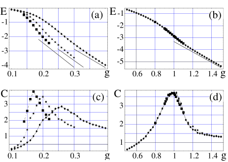
FIG. 1.: Internal energy $E$ and the fluctuation $C$ of the action with $\lambda=1$ vs non-local coupling $g$ for $N=8(\blacklozenge),16(\bigstar),24(\blacksquare)$; (a,c) PD model, (b,d) ED model. The solid lines in (a) and (b) are the large-$g$ expansion. In the PD model, strong $N$ dependence is observed in $E$ at large $g$ and in the developing peak of $C$. They indicate a second-order phase transition in the PD model.

$$E\equiv-\langle A_{\cal T}\rangle/V,\ \ C\equiv\langle(A_{\cal T}-\langle A_{\cal T}\rangle)^{2}\rangle/V.$$ (13)

For small $g$, the high-temperature expansion (HTE) gives $Z\simeq\exp[g^{2}(2Q_{2}+\lambda^{2})V]$ ($Q_{k}\equiv\sum_{\tau}c_{\tau}^{k}$), whereas for large $g$, the low-temperature expansion (LTE) around $V_{x,i,\tau}=1$ gives $Z\simeq\exp[(4gQ_{1}+2g\lambda-\log g)V]$.

In Fig.1, we present $E,C$ for $\lambda=1$ vs the nonlocal coupling $g$. They agree with the above HTE and LTE. In the PD model, $E$ of Fig.1(a) connects the HTE result and LTE result, showing that $V_{x,i,\tau}\sim 1$ for large $g$. $C$ of Fig.1(c) shows that its peak develops as $N$ increases. The finite-size scaling analysis shows $C$ of Fig.1(c) fits well in the form, $C(g,N)=N^{\sigma/\nu}\phi(N^{1/\nu}\epsilon),\epsilon=(g-g_{c})/g_{c}$ with $\nu=1.2\sim 1.3,\sigma/\nu=0.25\sim 0.26,g_{c}=0.10\sim 0.12.$ These results indicate that the PD model exhibits a second-order phase transition separating the disordered (confinement) phase and the ordered (deconfinement) phase at $g=g_{c}$. This transition will be confirmed later by the measurement of Polyakov lines. On the other hand, the peak of $C$ in the ED model does not develop as $N$ increases, showing no signals of a second-order transition. It may have a higher-order transition or just a crossover. Simulations of the models with $\lambda=0$ give similar behaviors of $E,C$, preserving the above phase structure for $\lambda=1$.

To study the nature of gauge dynamics, we calculated the spatial correlations of Polyakov lines $P_{x_{\bot}}$;

$$P_{x_{\bot}}=\prod_{x_{0}=1}^{N_{0}}U_{x_{\bot},x_{0},0},\ (x_{\bot}=(x_{1},x_{2})),$$ (14)

$$f_{P}(x_{\bot})=\langle\bar{P}_{x_{\bot}}P_{0}\rangle.$$ (15)

Since the present model (9) contains no long-range interactions in the spatial directions, $f_{P}(x_{\bot})$ is expected

FIG. 2.: Correlations of Polyakov lines, $f_{P}(x_{\bot})$, vs $|x_{\bot}|$. (a) PD ($\lambda=0$, N=16) with $g=0.4,0.3,0.2,0.1,0.02$ from above. (b) ED ($\lambda=0$, N=16) with $g=2.5,2.0,1.5,1.0,0.5$ from above. (c) and (d) show the order parameter $p=[f_{P}(x_{\bot}^{\rm MAX})]^{1/2}$ vs $g$ for the PD model; (c) $\lambda=0$ and (d) $\lambda=1$. They exhibit a long-range order for $g>g_{c}\simeq 0.15$ in the PD model.

to supply us with a good order parameter to detect a possible confinement-deconfinement transition. The deconfinement phase is characterized by small fluctuations of $U_{x\mu}$ and therefore by an order in $f_{P}(x_{\bot})$.

In Fig.2, we present $f_{P}(x_{\bot})$ with $\lambda=0$. The PD model of Fig.2(a) clearly exhibits an off-diagonal long-range order, i.e., $\lim_{x_{\bot}\rightarrow\infty}f_{P}(x_{\bot})\neq 0$ for $g\geq 0.20$, whereas the ED model of Fig.2(b) does not for all $g$’s. To see this explicitly, we plot in Fig.2(c,d) the order parameter $p\equiv[f_{P}(x_{\bot}^{\rm MAX})]^{1/2}$ for the PD model, where $x_{\bot}^{\rm MAX}\equiv N/\sqrt{2}$ is the distance at which $f_{P}$ becomes minimum due to the periodic boundary condition. $p$ starts to develop continuously from zero at $g=g_{c}\simeq 0.15$. The size dependence of $p$ shows a typical behavior of a second-order transition. Thus the gauge dynamics of the PD model is realized in the deconfinement phase for $g>g_{c}$, whereas it is in the confinement phase for $g<g_{c}$. In contrast, the ED model stays always in the confinement phase. These results including the value of $g_{c}$ are consistent with those derived from the data of $E,C$ in Fig.1.

To see the details of gauge dynamics, we measured the instanton density $\rho(x)$, an index for disorder of $U_{x\mu}$. We employ the definition of $\rho(x)$ in U(1) LGT by DeGrand and Toussaint [14]. For the local 3D compact U(1) LGT without matter fields, the average density $\rho=\langle\sum_{x}|\rho(x)|\rangle/V$ was measured in Ref.[15]. In Fig.3 we present $\rho$ vs $g$. It decreases as $g$ increases more rapidly in the PD model than in the ED model. This behavior of $\rho$ is consistent with the result that the PD model exhibits a second-order transition, while the ED model does not. The $\lambda$ coupling enhances the rate of decrease in $\rho$ as one expects since the spatial coupling favors the ordered deconfinement phase. In the ED model with $\lambda=1$, $\rho$ is fitted by $\propto\exp(-cg)$ with a constant $c$ in the dilute (large $g$) region, and the smooth increase for smaller $g$

FIG. 3.: Average instanton density $\rho$ vs $g$. (a)PD($\lambda=0$, $N=8$), (b)PD($\lambda=0$, $N=16$), (c)PD($\lambda=1$, $N=8$), (d)PD($\lambda=1$, $N=16$), (e)ED($\lambda=0$, $N=8,16$), (f)ED($\lambda=1$, $N=8,16$). The solid curve $\propto\exp(-cg)$ fits (f) at large $g$.

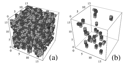
FIG. 4.: Snapshots of instanton configuration $\rho(x)$ for N=16. (a) PD($\lambda=1,g=0.15$) and (b) PD($\lambda=1,g=0.30$). The light cubes for $\rho(x)=1$ and the dark cubes for $\rho(x)=-1$.

indicates a crossover from the dilute gas of instantons to the dense gas, just the behavior similar to the case of pure and local LGT[6, 15].

In Fig.4 we show snapshots of $\rho(x)$ for the PD model with $\lambda=1$. Fig.4(a) is a dense gas and Fig.4(b) is a dilute gas. They are separated at $g_{c}\simeq 0.20$, the location of the peak of $C$ for $N=16$. In Fig.4(b), instantons mostly appear in dipole pairs at nearest-neighbor sites, $\rho(x)=1,\rho(x\pm\mu)=-1$, while in Fig.4(a), they appear densely and it is hard to determine their partners. In both cases, the distributions $\rho(x)$ have no apparent anisotoropies like column structures. However, the orientations of dipoles in Fig.4(b) are mostly ($\sim 92\%$) in the temporal direction as expected from Eq.(9).

For ordinary pure and local gauge systems, Wilson loop $W[{\cal C}]\equiv\langle\prod_{\cal C}U_{x\mu}\rangle$ along a closed loop ${\cal C}$ on the lattice is used as an order parameter to study the gauge dynamics; $W[C]$ obeys the area law in the confinement phase and the perimeter law in the deconfinement phase;

$$W[{\cal C}]\sim\left\{\begin{array}[]{ll}\exp(-aS[{\cal C}]),&{\rm area\ law},\\ \exp(-a^{\prime}L[{\cal C}]),&{\rm perimeter\ law},\end{array}\right.$$ (18)

where $S[{\cal C}]$ is the minimum area of a surface, the boundary of which is ${\cal C}$. For a local LGT containing matter fields, $W[{\cal C}]$ cannot be an order parameter because the matter fields generate the terms $\prod_{\cal C}U_{x\mu}$ with coeffcients $\sim\exp(-bL[{\cal C}])$ in the effective action. However, in the

FIG. 5.: Wilson loops ($N=32$) in the 1-2 plane at large $g$ vs $L[\cal C]$ or $S[\cal C]$. (a) PD($\lambda=1,g=0.25$), (b) ED($\lambda=1,g=1.5$). The PD model seems to prefer the perimeter law, whereas the ED model prefers the area law.

present model (9), the nonlocal terms are restricted only along the temporal direction, so it is interesting to measure $W[\cal C]$ for the loops lying in the spatial (1-2) plane.

In Fig.5, we plot $W[{\cal C}]$. For the PD model in Fig.5(a), the data at $g=0.25$ seem to prefer the perimeter law. For the ED model in Fig.5(b), the area law fits $W[{\cal C}]$ better than the perimeter law at $g=1.5$; a considerably larger value than $g\simeq 1.0$ at the peak of $C$. This suggests the area law holds in the ED model at all $g$. These observations are consistent with the previous results on the (non)existence of a phase transition. Wilson loops in the spatial plane are useful to study the gauge dynamics of the present model.

We have observed that the nonlocal couplings along the temporal direction in the PD model have sufficient effect of suppressing fluctuations of $U_{x\mu}$ to produce the deconfinement phase. This result strongly suggests a deconfinement transition in the original model (4) with massless matter fields, because the isotropically distributed nonlocal couplings of the original model should have similar effect. In such a possible deconfinement phase of the original model, perturbation theory may be applicable, which predicts the potential energy between two charges as $V(r)\sim r^{-1}$, a weaker one than the 3D Coulomb potential $V(r)\sim\log(r)$.

Let us turn to the nonrelativistic case. For the t-J model, by using the hopping expansion of holons and spinons at finite $T$ with the continuous imaginary time, we derived an effective gauge theory, which is highly nonlocal in the temporal direction. The obtained effective theory has a similar action as Eq.(9) with $c_{\tau}=$constant and $g\propto n$ where $n$ is the density of matter fields(holons and spinons)[8]. The nonlocal correlations of the effective gauge field like $c_{\tau}=$constant come from the fact that the nonrelativistic fermions contain a higher density of low-lying excitations compared to Dirac fermions, i.e., the existence of the Fermi surface (or line). Although the above effective gauge model is obtained for the system at finite $T$, we expect that a similar gauge model appears as an effective model at $T=0$. Then it is interesting and also important to investigate the gauge model (9) with $c_{\tau}=$constant, the nondecaying (ND) model. The ND model should shed some light on the anormalous normal state of cuprates because the Fermi line exists there.

We also made a Monte Caro simulation of the ND model, and obtained a phase transition similar to the PD model. However, the developing peak of $C$ shifts to smaller $g$ as $N$ increases more quickly than the PD model as $g_{c}\sim 0.1(N=8),0.045(N=16),0.03(N=24)$ for $\lambda=1$. It seems likely that $g_{c}\rightarrow 0$ as $N\rightarrow\infty$, that is, the deconfinement phase dominates for all $g(>0)$. This may be related with the diverging coefficient $Q_{2}(\propto N)$ in HTE, which implies that the radius of convergence is zero. This dominance of deconfienment phase of the ND model at $T=0$ may support the CSS at finite $T$, which is consistent with the result of Ref.[8]. In contrast to the ND model, the PD model has a finite limit of $Q_{2}(=1.645)$, and has a finite region $0\leq g\leq g_{c}$ of the confinement phase.

REFERENCES

-
[1]
J.B.Kogut and C.G.Strouthos,
Phys.Rev.D67, 034504
(2003) and references cited there in. -
[2]
G.Baskaran and P.W.Anderson, Phys.Rev.B37, 580(1988);
A.Nakamura and T.Matsui, Phys.Rev.B37, 7940(1988);
D.P. Arovas and A. Auerbach,
Phys.Rev.B38, 316(1988);
L.B.Ioffe and A.L.Larkin,Phys.Rev.B39, 8988(1989);
I.Ichinose and T.Matsui,Phys.Rev.B45, 9976(1992). - [3] I.Affleck and B.Marston, Phys.Rev.B37,3774(1988).
-
[4]
D.Yoshioka, G.Arakawa, I.Ichinose and T.Matsui,
Phys.Rev. B70, 174407(2004). - [5] I.Ichinose and T.Matsui, Phys.Rev.B68, 085322(2003) and references cited there in.
- [6] A.M.Polyakov, Nucl.Phys.B120, 429(1977).
- [7] P.W.Anderson, Phys.Rev.Lett.64,1839(1990).
-
[8]
I.Ichinose and T.Matsui,Nucl.Phys.B394, 281 (1993);
Phys.Rev.B51,11860(1995); Phys.Rev.Lett.86, 942(2001); I.Ichinose, T.Matsui and M.Onoda, Phys.Rev.B64, 104516 (2001). - [9] N.Nagaosa, Phys.Rev.Lett.71,4210(1993).
- [10] C.Nayak, Phys.Rev.Lett.85, 178(2000).
-
[11]
H.Kleinert, F.S.Nogueira, and A.Sudbø,
Phys.Rev.Lett.88, 232001(2002); Nucl.Phys.B666, 361(2003);
S. Kragset, A. Sudbø, and F. S. Nogueira, Phys. Rev. Lett. 92, 186403 (2004); K. Børkje, S. Kragset, and A. Sudbø, Phys. Rev. B 71, 085112 (2005);
F.S.Nogueira and H.Kleinert, cond-mat/0501022. -
[12]
I.F.Herbut and B.H.Seradjeh, Phys.Rev.Lett.91,
171601(2003); I.F.Herbut, B.H.Seradjeh, S.Sachdev, and G.Murthy, Phys.Rev.B68, 195110(2003); - [13] For the ED case, we used Eq.(12) instead of to make the comparison with the PD case more definitive.
- [14] T.A.DeGrand and D.Toussaint, Phys.Rev.D22,2478 (1980).
- [15] R.J.Wensley and J.D.Stack, Phys.Rev.Lett.63, 1764(1989).