Absorption and Emission Spectra of an higher-dimensional Reissner-Nordström black hole

Abstract

The absorption and emission problems of the brane-localized and bulk scalars are examined when the spacetime is a $(4+n)$-dimensional Reissner-Nordström black hole. Making use of an appropriate analytic continuation, we compute the absorption and emission spectra in the full range of particle’s energy. For the case of the brane-localized scalar the presence of the nonzero inner horizon parameter $r_{-}$ generally enhances the absorptivity and suppresses the emission rate compared to the case of the Schwarzschild phase. The low-energy absorption cross section exactly equals to $4\pi r_{+}^{2}$, two-dimensional horizon area. The effect of the extra dimensions generally suppresses the absorptivity and enhances the emission rate, which results in the disappearance of the oscillatory pattern in the total absorption cross section when $n$ is large. For the case of the bulk scalar the effect of $r_{-}$ on the spectra is similar to that in the case of the brane-localized scalar. The low-energy absorption cross section equals to the area of the horizon hypersurface. In the presence of the extra dimensions the total absorption cross section tends to be inclined with a positive slope. It turns out that the ratio of the missing energy over the visible one decreases with increase of $r_{-}$.

I Introduction

Black hole is an important physical system in a sense that we can formulate, test, and explore the quantum gravity, the untimate theory of physics, within this system. Although there is some doubt in the physical realization in the context of the information loss problem[1, 2], the most well-known quantum process in the black hole physics is a definitely Hawking radiation[3, 4]. Recently, therefore, there are various attempts to verify the Hawking effect by exploiting the analogue systems[5].

According to the Hawking formula the power spectrum, i.e. the energy emitted per unit time, is given by

$$\Gamma_{D}=\omega\frac{\sigma_{abs}(\omega)}{e^{\frac{\omega}{T_{H}}}\pm 1}\frac{d^{D-1}k}{(2\pi)^{D-1}}$$ (1)

where $D$ is a spacetime dimensions and $T_{H}$ is an Hawking temperature. The denominator is a Planck factor, and the upper and lower signs correspond to the fermion and boson, respectively. The appearance of the Planck factor in the emission spectrum indicates that the black hole is a thermal object. The numerator $\sigma_{abs}(\omega)$ is a total absorption cross section which is a sum of the partial absorption cross section $\sigma_{\ell}(\omega)$;

$$\sigma_{abs}(\omega)=\sum_{\ell}\sigma_{\ell}(\omega).$$ (2)

Although the summation index $\ell$ represents, in general, the set of all quantum numbers, this becomes the orbital quantum number for the spherically symmetric black holes, which is the case in this paper. The partial absorption cross section $\sigma_{\ell}(\omega)$ in $D$-dimensions is expressed in the form[6]

$$\sigma_{\ell}(\omega)=\tilde{A}_{H}\frac{2^{D-4}\Gamma^{2}\left(\frac{D-1}{2}\right)}{\pi(\omega vr_{H})^{D-2}}\frac{(2\ell+D-3)(\ell+D-4)!}{(D-3)!\ell!}{\cal T}_{\ell}(\omega)$$ (3)

where $\tilde{A}_{H}$ is an area of the horizon

$$\tilde{A}_{H}=\frac{2\pi^{\frac{D-1}{2}}}{\Gamma\left(\frac{D-1}{2}\right)}r_{H}^{D-2}.$$ (4)

The factor $v$ in Eq.(3) is a velocity factor defined $v=\sqrt{1-m^{2}/\omega^{2}}$, where $m$ is a particle mass. ${\cal T}_{\ell}(\omega)$ is a transmission coefficient, which is a transmission probability for the incident ingoing wave shooted from the asymptotic region. Since this factor should be dependent on the potential generated by the horizon structure, it encodes a valuable information for the nature of spacetime. Since, furthermore, ${\cal T}_{\ell}(\omega)\neq 1$ in general, this factor makes the black hole distinct from the black body. In this reason the factor is often called ‘greybody’ factor.

As Eq.(1) indicates, the absorption cross section plays an important role for understanding the emission spectrum. Many computational techniques for the calculation of the absorption cross section were developed about three decades ago[7, 8, 9, 10, 11, 12, 13]. The computational procedure most peoples adopted is a matching between the near-horizon and the asymptotic solutions. Following this procedure, Unruh[12] derived the low-energy absorption cross section analytically for the massive scalar and Dirac fermion in the $4d$ Schwarzschild background. For the scalar case the low-energy cross section $\sigma_{S}$ coincides with $\sigma_{S}=A_{H}/v$ when we take a s-wave, where $A_{H}$ is an area of horizon and $v$ is a velocity factor. This means the low-energy cross section for the s-wave is equal to the horizon area in the massless limit. It was also found by Unruh that the low-energy cross section $\sigma_{F}$ for the massive Dirac fermion bacomes $\sigma_{F}=\sigma_{S}/8$ when we take $j=1/2$, where $j$ is a total angular momentum. Recently, this ratio factor is generalized to $2^{(n-3)/(n+1)}$ in the $(4+n)$-dimensional Schwarzschild phase.

The fact that the low-energy absorption cross section for the s-wave massless scalar equals to the horizon area is generally proved in the higher-dimensional asymptotically flat and spherically symmetric black holes[14]. This universal property was re-examined in the $p$-brane-like object[15, 16, 17] and non-spherically symmetric black hole such as the three-dimensional BTZ black hole[19].

The absorption and emission problems for the full range of particle’s energy were also computed by applying the quantum mechanical scattering theories[13, 20, 21]. Adopting an appropriate numerical techniques, it was found that the total absorption cross section with respect to the particle’s energy generally exhibits a wiggly pattern, which implies that each partial absorption cross section has a peak in different energy scale. However, the total emission rate does not have the oscillatory pattern, which indicates that the Planck factor in general suppresses the contribution of the higher partial waves except s-wave. It turned out also that the scalar mass reduces the emission rate.

Besides the general relativity black holes are important physical laboratories in other theoretical branches such as the string theories and the brane-world scenarios. In string theories the attempt to understand the Bekenstein-Hawking entropy[22, 23], one quarter of the horizon, microscopically was initiated in Ref.[24]. Ref.[24] used the five-dimensional extremal black hole by counting the degeneracy of the Bogomol’ni-Prasad-Sommerfield(BPS)-saturated D-brane bound states. Later, this is extended to the certain near-extremal states[25]. Subsequently, the correspondence between the black hole and D-brane was focused to the decay-rate via the Hawking radiation[26]. In Ref.[27] five-dimensional Reissner-Nordström(RN) black hole carrying three different electric charges was chosen to test the correspondence. In particular, Ref.[27] showed the exact coincidence between the semi-classical black hole approach and D-brane approach in the absorption and emission rates of the neutral and charged scalars in the dilute gas region. These calculations were extended to the absorption and emission problems for the particles with arbitrary spin[28]. However, it is not clear whether the exact agreement between these two different approaches is maintained beyond the dilute gas region or not. The possibility for the disagreement was argued in Ref.[29] in the near-extremal range slightly different from the dilute gas region although the rigorous proof was not given yet.

The emergence for the TeV-scale gravity in the brane-world scenario such as the large extra dimensions[30, 31] or warped extra dimensions[32] opens the possibility to make tiny black holes factory in the future high-energy colliders[33, 34, 35, 36]. In this context it is important to study the absorption and emission problems of the higher-dimensional black holes for the future experiments. Recently, works along this direction were done[18, 37, 38, 39, 40, 41]. Especially, Ref.[18] showed that the ratio factor $\sigma_{F}/\sigma_{S}=1/8$[12] in the four-dimensional Schwarzschild black hole is changed into $\sigma_{F}/\sigma_{S}=2^{(n+3)/(n+1)}$ in $(4+n)$ dimension. Thus this ratio factor may give an evidence for the existence of the extra dimensions in the future black hole experiments.

In this paper we would like to compute the absorption and emission spectra numerically for the brane-localized scalar and bulk scalar in the full-range of energy when the spacetime is a $(4+n)$-dimensional RN black hole[42, 43]

$$ds^{2}=-\left[1-\left(\frac{\tilde{r}_{+}}{\tilde{r}}\right)^{n+1}\right]\left[1-\left(\frac{\tilde{r}_{-}}{\tilde{r}}\right)^{n+1}\right]dt^{2}+\frac{d\tilde{r}^{2}}{\left[1-\left(\frac{\tilde{r}_{+}}{\tilde{r}}\right)^{n+1}\right]\left[1-\left(\frac{\tilde{r}_{-}}{\tilde{r}}\right)^{n+1}\right]}+\tilde{r}^{2}d\Omega_{n+2}^{2}$$ (5)

where

$$d\Omega_{n+2}^{2}=d\theta_{n+1}^{2}+\sin^{2}\theta_{n+1}\Bigg{(}d\theta_{n}^{2}+\sin^{2}\theta_{n}\bigg{(}\cdots+\sin^{2}\theta_{2}\left(d\theta_{1}^{2}+\sin^{2}\theta_{1}d\varphi^{2}\right)\cdots\bigg{)}\Bigg{)}.$$ (6)

It is well-known that the mass $M$, charge $Q$, entropy $S$ and Hawking temperature $T_{H}$ of the spacetime (5) are

$$M = \frac{n+2}{16\pi}\Omega_{n+2}\left(r_{+}^{n+1}+r_{-}^{n+1}\right)$$ (7)

$$Q = \pm\left(r_{+}r_{-}\right)^{\frac{n+1}{2}}\sqrt{\frac{(n+1)(n+2)}{8\pi}}$$ (8)

$$S = \frac{1}{4}\Omega_{n+2}r_{+}^{n+2}$$ (9)

$$T_{H} = \frac{n+1}{4\pi r_{+}^{n+2}}\left(r_{+}^{n+1}-r_{-}^{n+1}\right)$$ (10)

where

$$\Omega_{n+2}=\frac{2\pi^{\frac{n+3}{2}}}{\Gamma\left(\frac{n+3}{2}\right)}$$ (11)

is the area of a unit $(n+2)$-sphere.

In this paper we will take an arbitrary $r_{-}$, which enables us to treat the Schwarzschild and extremal black holes as an unified way. Although our paper is strongly motivated by the recent brane-world scenarios, our treatment of the inner-horizon parameter $r_{-}$ may give some insight into the black hole-D-brane correspondence beyond the dilute gas domain.

This paper is organized as following. In section II the general properties of the scalar wave equation for the brane-localized scalar are examined. The effective potential, Wronskian between two independent solutions and any other physical quantities are explicitly computed. Two solutions which are convergent in the near-horizon and asymptotic regimes respectively are derived as an analytic form. In section III the absorption and emission spectra for the brane-localized scalar is computed numerically by applying the quantum mechanical scattering theories. To carry out a calculation the solution which has a convergent range around $r=b$ where is $b$ is some parameter is constructed. Using this solution the near-horizon solution is matched with asymptotc solution via the analytic continuation. It turns out that the presence of the nonzero inner horizon parameter $r_{-}$ generally enhances the absorptivity and suppresses the emission rate compared to the case of the Schwarzschild phase. The effect of the extra dimensions generally suppresses the absorption rate, which results in the disappearance of the oscillatory pattern in the total absorption cross section. In section IV the general properties of the wave equation for the bulk scalar is examined. As in section II all physical quantities are expressed in terms of the jost functions. The analytic near-horizon and asymptotic solutions are explicitly derived. The numerical approach for the absorption and emission spectra of the bulk scalar is discussed in next section. The effect of $r_{-}$ on the spectra is similar to that for the case of the brane-localized scalar. However, the universality of the s-wave cross section makes the oscillatory pattern in the total absorption cross section to be maintained. A remarkable fact in the presence of the extra dimensions is that the total absorption cross section tends to be inclined with a positive slope. The slope seems to increase with increasing $n$. In section VI the ratio of the missing energy, i.e. emission into the bulk, over the visible one are discussed. It turns out that this ratio factor decreases with increasing $r_{-}$. When $n$ is not too large, the ratio factor is smaller than unity, which indicates that the emission into the brane is dominant. This is consistent with the main result of Ref.[45]. If, however, $n$ is very large, the emission into the bulk can be dominant. In section VII a brief conclusion is given.

II wave equation for the brane-localized scalar

In this section we would like to examine the various properties of the wave equation for the brane-localized scalar $\Phi_{BR}$ minimally coupled to the spacetime (5). Thus we should assume that $\Phi_{BR}$ is a function of the brane worldvolume coordinate, i.e. $\Phi_{BR}=\Phi_{BR}(t,r,\theta\equiv\theta_{n+1},\varphi)$. Furthermore, we assume that the $3$-brane is located at $\theta_{1}=\theta_{2}=\cdots=\theta_{n}=\pi/2$, where $\theta_{1},\theta_{2},\cdots$ and $\theta_{n}$ are toroidally compactified extra dimensions. Thus the induced metric on the brane is

$$ds_{4}^{2}=-h_{n}(r)dt^{2}+\frac{1}{h_{n}(r)}dr^{2}+r^{2}(d\theta^{2}+\sin^{2}\theta d\varphi^{2})$$ (12)

where $h_{n}(r)=h_{n,+}(r)h_{n,-}(r)$ and $h_{n,\pm}(r)=1-(r_{\pm}/r)^{n+1}$.

Using a separability condition $\Phi_{BR}=e^{-i\omega t}R_{\ell}(r)Y_{\ell,\tilde{m}}(\theta,\varphi)$, it is easy to show that the wave equation $(\Box-m^{2})\Phi_{BR}=0$ reduces to the following radial equation

$$x(x^{n+1}-x_{+}^{n+1})^{2}(x^{n+1}-x_{-}^{n+1})^{2}\frac{d^{2}R}{dx^{2}}+(x^{n+1}-x_{+}^{n+1})(x^{n+1}-x_{-}^{n+1})$$ (13)

$$\hskip 14.22636pt\times\left[(n+1)x^{n+1}(2x^{n+1}-x_{+}^{n+1}-x_{-}^{n+1})-2n(x^{n+1}-x_{+}^{n+1})(x^{n+1}-x_{-}^{n+1})\right]\frac{dR}{dx}$$ (14)

$$\hskip 56.9055pt+\Bigg{[}x^{4n+5}-\ell(\ell+1)x^{2n+1}(x^{n+1}-x_{+}^{n+1})(x^{n+1}-x_{-}^{n+1})$$ (15)

$$\hskip 113.81102pt+\frac{m^{2}}{\omega^{2}v^{2}}x^{2n+3}\left\{x^{n+1}(x_{+}^{n+1}+x_{-}^{n+1})-x_{+}^{n+1}x_{-}^{n+1}\right\}\Bigg{]}R=0$$ (16)

where $v=\sqrt{1-m^{2}/\omega^{2}}$, $x\equiv\omega vr$ and $x_{\pm}\equiv\omega vr_{\pm}$. From now on we take the massless case ($m=0$) for simplicity.

From Eq.(13) it is straightforward to derive the following Schrödinger-like equation

$$-\frac{d^{2}\psi}{dr_{*}^{2}}+V_{eff}^{BR}\psi=\omega^{2}\psi$$ (17)

where $\psi\equiv rR$ and the tortoise coordinate $r_{*}$ is

$$r_{*}=\int\frac{dr}{h_{n}(r)}.$$ (18)

The effective potential $V_{eff}^{BR}$ in Eq.(17) is

$$V_{eff}^{BR}=\frac{h_{n}(r)}{r^{2}}\left[\ell(\ell+1)+(n+1)\left\{h_{n,+}(r)+h_{n,-}(r)-2h_{n}(r)\right\}\right].$$ (19)

Although it seems to be impossible to carry out the integration in Eq.(18) for the arbitrary $n$, we can easily infer the behavior of the tortoise coordinate in the near-horizon and asymptotic regimes

$$\lim_{r\rightarrow r_{+}}r_{*}\sim\frac{r_{+}}{(n+1)h_{n,-}(r_{+})}\ln(r-r_{+}),\hskip 56.9055pt\lim_{r\rightarrow\infty}r_{*}\sim r.$$ (20)

For $n=0$, $1$, and $2$ the explicit expressions of $r_{*}$ are

$$r_{*} = r+\frac{1}{r_{+}-r_{-}}\left[r_{+}^{2}\ln(r-r_{+})-r_{-}^{2}\ln(r-r_{-})\right]\hskip 108.12054pt\mbox{(n=0)}$$ (21)

$$r_{*} = r+\frac{1}{2(r_{+}^{2}-r_{-}^{2})}\left[r_{+}^{3}\ln\frac{r-r_{+}}{r+r_{+}}-r_{-}^{3}\ln\frac{r-r_{-}}{r+r_{-}}\right]\hskip 102.43008pt\mbox{(n=1)}$$ (22)

$$r_{*} = r+\frac{1}{3(r_{+}^{3}-r_{-}^{3})}\left[r_{+}^{4}\ln\frac{r-r_{+}}{\sqrt{r^{2}+r_{+}r+r_{+}^{2}}}-r_{-}^{4}\ln\frac{r-r_{-}}{\sqrt{r^{2}+r_{-}r+r_{-}^{2}}}\right]$$ (24)

$$\hskip 28.45274pt-\frac{1}{\sqrt{3}(r_{+}^{3}-r_{-}^{3})}\left[r_{+}^{4}\tan^{-1}\frac{2r+r_{+}}{\sqrt{3}r_{+}}-r_{-}^{4}\tan^{-1}\frac{2r+r_{-}}{\sqrt{3}r_{-}}\right].\hskip 28.45274pt\mbox{(n=2)}$$

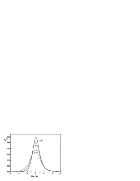
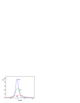
FIG. 1.: (a) Plot of the effective potential $V_{eff}^{BR}$ with respect to the tortoise coordinate $r_{*}$ for $r_{-}=0$, $0.4$ and $0.7$ when $n=1$, $\ell=0$ and $r_{+}=1$. This figure indicates the absorption cross section enhances when $r_{-}$ approaches to the extremal limit. This fact can be deduced also from the Hawking temperature. (b) Plot of the effective potential $V_{eff}^{BR}$ with respect to the tortoise coordinate $r_{*}$ for $n=0$, $1$ and $2$ when $r_{-}=0.4$, $r_{+}=1$ and $\ell=0$. This figure indicates that the absorption ability of black hole may be suppressed with increase of $n$. This can be understood from the monotonically decreasing behavior of the critical radius $r_{c}$ with respect to $n$.

Fig. 1(a) is a plot of $V_{eff}^{BR}$ at $r_{-}=0$, $0.4$, and $0.7$. This figure shows the barrier height becomes lower when the inner horizon parameter $r_{-}$ increases. This implies that the absorptivity of the black hole should enhance with increase of $r_{-}$. This fact can be conjectured by Hawking temperature in Eq.(7). The Hawking temperature with fixed $r_{+}$ has a maximum $(n+1)/4\pi r_{+}$ at the Schwarzschild limit and becomes lower and lower with increase of $r_{-}$, and eventually goes to zero in the extremal limit. Since the frozen matter in general absorbs something easily but does not emit well to move to the equilibrium state, one can understand Fig. 1(a) from the Hawking temperature. Fig. 1(b) is a plot of $V_{eff}^{BR}$ at $n=0$, $1$, and $2$ when $r_{-}=0.4$. This figure shows the barrier height becomes higher when the number of the extra dimensions increases, which indicates that the absorption cross section decreases with increase of $n$. This can be understood from the fact that the critical radius $r_{c}\equiv\sqrt{\sigma_{\infty}/\pi}$, where $\sigma_{\infty}$ is an high-energy limit of the total cross section, monotonically decreases with increase of $n$[45].

Another property of the radial equation (13) is its real nature: if $R$ is a solution of (13), $R^{*}$ is a solution too. The Wronskian of $R$ and $R^{*}$ can be evaluated from Eq.(13);

$$W[R^{*},R]_{x}\equiv R^{*}\frac{dR}{dx}-R\frac{dR^{*}}{dx}=\frac{C_{n}x^{2n}}{(x^{n+1}-x_{+}^{n+1})(x^{n+1}-x_{-}^{n+1})}$$ (25)

where $C_{n}$ is a $n$-dependent integration constant.

Now, we would like to derive the solutions of the radial equation (13). The solution which is convergent around the near-horizon region can be expanded as

$${\cal G}_{n,\ell}(x,x_{+},x_{-})=e^{\lambda_{n}\ln|x-x_{+}|}\sum_{N=0}^{\infty}d_{\ell,N}(x-x_{+})^{N}$$ (26)

where $\lambda_{n}$ is a $n$-dependent pure imaginary quantity

$$\lambda_{n}=-i\frac{x_{+}^{n+2}}{(n+1)(x_{+}^{n+1}-x_{-}^{n+1})}.$$ (27)

When $n=0$, $d_{\ell,N}$ satisfies the following recursion relation

$$\hskip 56.9055ptd_{\ell,N}\left[(x_{+}-x_{-})^{2}(N+\lambda_{0})^{2}+x_{+}^{4}\right]$$ (28)

$$+d_{\ell,N-1}\left[(N+\lambda_{0}-1)(2N+2\lambda_{0}-1)(x_{+}-x_{-})+4x_{+}^{3}-\ell(\ell+1)(x_{+}-x_{-})\right]$$ (29)

$$+d_{\ell,N-2}\left[(N+\lambda_{0}-1)(N+\lambda_{0}-2)+6x_{+}^{2}-\ell(\ell+1)\right]+4x_{+}d_{\ell,N-3}+d_{\ell,N-4}=0.$$ (30)

In appendix A we will present the recursion relation for $n=1$ case. Although similar relations can be derived for $n\geq 2$, they are very lengthy and thus the explicit expressions will not be given in this paper.

The solutions of Eq.(13) which are convergent in the asymptotic region can be also expanded as

$${\cal F}_{n,\ell(\pm)}(x,x_{+},x_{-})=(\pm i)^{\ell+1}e^{\mp ix}(x-x_{+})^{\pm\lambda_{n}}\sum_{N=0}^{\infty}\tau_{N(\pm)}x^{-(N+1)}$$ (31)

where ${\cal F}_{n,\ell(+)}$ and ${\cal F}_{n,\ell(-)}$ are ingoing and outgoing solutions respectively. It is worthwhile noting that ${\cal F}_{n,\ell(+)}$ is a complex conjugate of ${\cal F}_{n,\ell(-)}$. The coefficient $\tau_{N(-)}$ satisfies the following recursion relation when $n=0$:

$$\hskip 56.9055pt[C_{1}-2i(N+1)]\tau_{N(-)}+[N(N+1)-B_{1}N+C_{2}]\tau_{N-1(-)}$$ (32)

$$+[A_{1}(N-1)N-B_{2}(N-1)+C_{3}]\tau_{N-2(-)}+[A_{2}(N-2)(N-1)-B_{3}(N-2)+C_{4}]\tau_{N-3(-)}$$ (33)

$$\hskip 28.45274pt+[A_{3}(N-3)(N-2)-B_{4}(N-3)]\tau_{N-4(-)}+A_{4}(N-4)(N-3)\tau_{N-5(-)}=0$$ (34)

where $\tau_{0(-)}=1$, $\tau_{N(+)}=\tau_{N(-)}^{*}$, and

$$A_{1}=-2(x_{+}+x_{-})\hskip 85.35826ptA_{2}=x_{+}^{2}+4x_{+}x_{-}+x_{-}^{2}$$ (35)

$$A_{3}=-2x_{+}x_{-}(x_{+}+x_{-})\hskip 56.9055ptA_{4}=x_{+}^{2}x_{-}^{2}$$ (36)

$$B_{1}=2\left(1-i\frac{x_{+}^{2}-2x_{-}^{2}}{x_{+}-x_{-}}\right)\hskip 51.21504ptB_{2}=-3(x_{+}+x_{-})+2i\frac{x_{-}(x_{+}^{2}-3x_{+}x_{-}-x_{-}^{2})}{x_{+}-x_{-}}$$ (37)

$$B_{3}=(x_{+}^{2}+4x_{+}x_{-}+x_{-}^{2})+2i\frac{x_{+}x_{-}^{2}(x_{+}+2x_{-})}{x_{+}-x_{-}}\hskip 28.45274ptB_{4}=-x_{+}x_{-}(x_{+}+x_{-})-2i\frac{x_{+}^{2}x_{-}^{3}}{x_{+}-x_{-}}$$ (38)

$$C_{1}=-\frac{2x_{-}^{2}}{x_{+}-x_{-}}+2i\hskip 42.67912ptC_{2}=\left[\frac{x_{-}^{2}(2x_{+}^{2}-2x_{+}x_{-}-x_{-}^{2})}{(x_{+}-x_{-})^{2}}-\ell(\ell+1)\right]-i\frac{2x_{+}^{2}-3x_{-}^{2}}{x_{+}-x_{-}}$$ (39)

$$C_{3}=\left[\frac{2x_{+}x_{-}^{4}}{(x_{+}-x_{-})^{2}}+\ell(\ell+1)(x_{+}+x_{-})\right]+i\frac{x_{-}(2x_{+}^{2}-3x_{+}x_{-}-x_{-}^{2})}{x_{+}-x_{-}}$$ (40)

$$C_{4}=-\left[\frac{x_{+}^{2}x_{-}^{4}}{(x_{+}-x_{-})^{2}}+\ell(\ell+1)x_{+}x_{-}\right]+i\frac{x_{+}x_{-}^{3}}{x_{+}-x_{-}}.$$ (41)

The recursion relation for $n=1$ case is explicitly given in appendix A.

Using Eq.(25) it is easy to show

$$W[{\cal G}_{n,\ell}^{*},{\cal G}_{n,\ell}]_{x}\equiv{\cal G}_{n,\ell}^{*}\partial_{x}{\cal G}_{n,\ell}-{\cal G}_{n,\ell}\partial_{x}{\cal G}_{n,\ell}^{*}=\frac{-2i|g_{n,\ell}|^{2}x_{+}^{2}x^{2n}}{(x^{n+1}-x_{+}^{n+1})(x^{n+1}-x_{-}^{n+1})}$$ (42)

$$W[{\cal F}_{n,\ell(+)},{\cal F}_{n,\ell(-)}]_{x}\equiv{\cal F}_{n,\ell(+)}\partial_{x}{\cal F}_{n,\ell(-)}-{\cal F}_{n,\ell(-)}\partial_{x}{\cal F}_{n,\ell(+)}=\frac{2ix^{2n}}{(x^{n+1}-x_{+}^{n+1})(x^{n+1}-x_{-}^{n+1})}$$ (43)

where $g_{n,\ell}\equiv d_{\ell,0}$.

Now, we would like to show how the coefficient $g_{n,\ell}$ is related to the partial scattering amplitude. Since the real scattering solution, say $R_{n,\ell}$, should be ingoing wave at the near-horizon region and mixture of ingoing and outgoing waves at the asymptotic region, we can express it in the form

$$R_{n,\ell}\stackrel{{\scriptstyle x\rightarrow x_{+}}}{{\sim}}g_{n,\ell}(x-x_{+})^{\lambda_{n}}\left[1+O(x-x_{+})\right]$$ (44)

$$R_{n,\ell}\stackrel{{\scriptstyle x\rightarrow\infty}}{{\sim}}i^{\ell+1}\frac{2\ell+1}{2x}\left[e^{-ix+\lambda_{n}\ln|x-x_{+}|}-(-1)^{\ell}S_{n,\ell}(x_{+},x_{-})e^{ix-\lambda_{n}\ln|x-x_{+}|}\right]+O\left(\frac{1}{x^{2}}\right)$$ (45)

where $S_{n,\ell}$ is a partial scattering amplitude. If we define a phase shift $\delta_{n,\ell}$ as $S_{n,\ell}\equiv e^{2i\delta_{n,\ell}}$, the second equation of Eq.(44) can be written as

$$R_{n,\ell}\stackrel{{\scriptstyle x\rightarrow\infty}}{{\sim}}\frac{2\ell+1}{x}e^{i\delta_{n,\ell}}\sin\left[x+i\lambda_{n}\ln|x-x_{+}|-\frac{\pi}{2}\ell+\delta_{n,\ell}\right]+O\left(\frac{1}{x^{2}}\right).$$ (46)

Next let us consider the Wronskian $W[R_{n,\ell}^{*},R_{n,\ell}]_{x}\equiv R_{n,\ell}^{\ast}\partial_{x}R_{n,\ell}-R_{n,\ell}\partial_{x}R_{n,\ell}^{\ast}$. From the first equation of Eq.(44) it is straightforward to show $W[R_{n,\ell}^{*},R_{n,\ell}]_{x}=W[{\cal G}_{n,\ell}^{*},{\cal G}_{n,\ell}]_{x}$ while Eq.(46) makes the Wronskian in the form

$$W[R_{n,\ell}^{*},R_{n,\ell}]_{x}=\frac{-i(2\ell+1)^{2}x^{2n}}{(x^{n+1}-x_{+}^{n+1})(x^{n+1}-x_{-}^{n+1})}e^{-2\beta_{n,\ell}}\sinh 2\beta_{n,\ell}$$ (47)

where $\delta_{n,\ell}$ is assumed as $\delta_{n,\ell}\equiv\eta_{n,\ell}+i\beta_{n,\ell}$. Therefore, equating those two Wronskians yield a relation

$$|g_{n,\ell}|^{2}=\frac{\left(\ell+\frac{1}{2}\right)^{2}}{x_{+}^{2}}\left(1-e^{-4\beta_{n,\ell}}\right).$$ (48)

Since $1-e^{-4\beta_{n,\ell}}=1-|S_{n,\ell}(x_{+},x_{-})|^{2}$ is a transmission coefficient, we can compute the absorption cross section using Eq.(3) if we know $g_{n,\ell}$.

Next we would like to discuss how to compute $g_{n,\ell}$ by matching the asymptotic solution (31) with the near-horizon solution (26). In order to discuss it properly it is convenient[13, 21] to introduce a new wave solution $\tilde{R}_{n,\ell}(x,x_{+},x_{-})$, which differs from $R_{n,\ell}(x,x_{+},x_{-})$ in its normalization. It is normalized in such a way that

$$\tilde{R}_{n,\ell}(x,x_{+},x_{-})\stackrel{{\scriptstyle x\rightarrow x_{+}}}{{\sim}}(x-x_{+})^{\lambda_{n}}\left[1+O(x-x_{+})\right].$$ (49)

Since ${\cal F}_{n,\ell(\pm)}$ in Eq.(31) are two linearly independent solutions of the radial equation (13), one may write $\tilde{R}_{n,\ell}$ as a combination of them

$$\tilde{R}_{n,\ell}(x,x_{+},x_{-})=f_{n,\ell}^{(-)}(x_{+},x_{-}){\cal F}_{n,\ell(+)}(x,x_{+},x_{-})+f_{n,\ell}^{(+)}(x_{+},x_{-}){\cal F}_{n,\ell(-)}(x,x_{+},x_{-})$$ (50)

where the coefficients $f_{n,\ell}^{(\pm)}(x_{+},x_{-})$ are called the jost functions. Using Eq.(42) one can compute $f_{n,\ell}^{(\pm)}$ as following:

$$f_{n,\ell}^{(\pm)}(x_{+},x_{-}) = \pm\frac{(x^{n+1}-x_{+}^{n+1})(x^{n+1}-x_{-}^{n+1})}{2ix^{2n}}W[{\cal F}_{n,\ell(\pm)},\tilde{R}]_{x}$$ (51)

$$= \pm\frac{\omega(r^{n+1}-r_{+}^{n+1})(r^{n+1}-r_{-}^{n+1})}{2ir^{2n}}W[{\cal F}_{n,\ell(\pm)},\tilde{R}]_{r}.$$ (52)

Inserting the explicit form of ${\cal F}_{n,\ell(\pm)}$ into Eq. (50) and comparing it with the asymptotic expression of $R_{n,\ell}$ in Eq. (44), one can easily derive the following two relations

$$S_{n,\ell}(x_{+},x_{-}) = \frac{f_{n,\ell}^{(+)}(x_{+},x_{-})}{f_{n,\ell}^{(-)}(x_{+},x_{-})}$$ (53)

$$f_{n,\ell}^{(-)}(x_{+},x_{-}) = \frac{\ell+\frac{1}{2}}{g_{n,\ell}(x_{+},x_{-})}.$$ (54)

Thus once we know the jost functions, we can compute the scattering quantities such as $S_{n,\ell}(x_{+},x_{-})$ and $g_{n,\ell}(x_{+},x_{-})$. Combining Eq.(48) and (53), we can express the greybody factor in terms of the jost function

$$1-|S_{n,\ell}(x_{+},x_{-})|^{2}=\frac{x_{+}^{2}}{|f_{n,\ell}^{(-)}(x_{+},x_{-})|^{2}}.$$ (55)

Since the relation between the absorption cross section $\sigma_{n,\ell}^{BR}$ and the greybody factor for the brane-localized scalar is given in Eq.(3) with fixing $D=4$, it is easy to show

$$\sigma_{n,\ell}^{BR}=\frac{\pi}{\omega^{2}}(2\ell+1)\left[1-|S_{n,\ell}(x_{+},x_{-})|^{2}\right]=\frac{\pi(2\ell+1)r_{+}^{2}}{|f_{n,\ell}^{(-)}(x_{+},x_{-})|^{2}}.$$ (56)

Thus one can compute the absorption cross section from the jost function $f_{n,\ell}^{(-)}(x_{+},x_{-})$. In next section we will compute the jost functions numerically by applying the analytic continuation.

III Absorption and Emission for the brane-localized scalar

In this section we will compute the jost functions $f_{n,\ell}^{(\pm)}(x_{+},x_{-})$ numerically. The computational procedure is as following. Firstly, we note that $\tilde{R}_{n,\ell}(x,x_{+},x_{-})$ defined in Eq.(49) can be obtained from ${\cal G}_{n,\ell}(x,x_{+},x_{-})$ by $\tilde{R}_{n,\ell}(x,x_{+},x_{-})={\cal G}_{n,\ell}(x,x_{+},x_{-})|_{d_{\ell,0}=1}$. This can be understood from a convergent expansion around the near-horizon region. The other expression (50) is of course a convergent expansion around the asymptotic region. Since, however, the domains of convergence for those two expressions are different, we cannot use them directly for the computation of the jost functions. In other words, we need two expressions which have common domain of convergence. This is achieved by analytic continuation. The solution which is a power series in the neighborhood of an arbitrary point $x=b$ can be straightforwardly obtained from the radial equation (13), whose formal form is

$$\varphi_{n,\ell}(x,x_{+},x_{-})=(x-x_{+})^{\lambda_{n}}\sum_{N=0}^{\infty}D_{N}(x-b)^{N}.$$ (57)

For $n=0$ the coefficient $D_{N}$ satisfies the following recursion relation:

$$\tilde{A}_{4}(N+5)(N+6)D_{N+6}+\left[\tilde{A}_{3}(N+4)(N+5)+\tilde{B}_{3}(N+5)\right]D_{N+5}$$ (58)

$$\hskip 56.9055pt+\left[\tilde{A}_{2}(N+3)(N+4)+\tilde{B}_{2}(N+4)+\tilde{C}_{4}\right]D_{N+4}$$ (59)

$$\hskip 56.9055pt+\left[\tilde{A}_{1}(N+2)(N+3)+\tilde{B}_{1}(N+3)+\tilde{C}_{3}\right]D_{N+3}$$ (60)

$$+\left[(N+1)(N+2)+2(\lambda_{0}+1)(N+2)+\tilde{C}_{2}\right]D_{N+2}+\tilde{C}_{1}D_{N+1}+D_{N}=0$$ (61)

where

$$\tilde{A}_{1}=2\left[(b-x_{+})+(b-x_{-})\right]\hskip 28.45274pt\tilde{A}_{2}=(b-x_{+})^{2}+4(b-x_{+})(b-x_{-})+(b-x_{-})^{2}$$ (62)

$$\tilde{A}_{3}=(b-x_{+})^{2}(b-x_{-})^{2}\hskip 28.45274pt\tilde{B}_{1}=(2\lambda_{0}+3)(b-x_{+})+(4\lambda_{0}+3)(b-x_{-})$$ (63)

$$\tilde{B}_{2}=(b-x_{+})^{2}+4(\lambda_{0}+1)(b-x_{+})(b-x_{-})+(2\lambda_{0}+1)(b-x_{-})^{2}$$ (64)

$$\tilde{B}_{3}=(b-x_{+})(b-x_{-})\left[(b-x_{+})+(2\lambda_{0}+1)(b-x_{-})\right]\hskip 28.45274pt\tilde{C}_{1}=4b$$ (65)

$$\tilde{C}_{2}=\lambda_{0}(\lambda_{0}+1)+6b^{2}-\ell(\ell+1)$$ (66)

$$\tilde{C}_{3}=\left[\lambda_{0}-\ell(\ell+1)\right](b-x_{+})+\left[\lambda_{0}(2\lambda_{0}+1)-\ell(\ell+1)\right](b-x_{-})+4b^{3}$$ (67)

$$\tilde{C}_{4}=\lambda_{0}^{2}(b-x_{-})^{2}+\left[\lambda_{0}-\ell(\ell+1)\right](b-x_{+})(b-x_{-})+b^{4}.$$ (68)

The recursion relation for $n=1$ is explicitly given in appendix A. The recursion relation for each $n$ enables us to compute all the $D_{N}$’s ($N\geq 2$) in terms of $D_{0}$ and $D_{1}$. Since $D_{0}$ and $D_{1}$ are expressed in terms of $\varphi_{n,\ell}(b)$ and $\partial_{x}\varphi_{n,\ell}(b)$, the analytic continuation can be directly achieved. In actual computer calculation the asymptotic region is identified by $r\sim 1000$ and the analytic continuation procedure is repeated over and over to make a common domain of convergence.

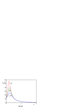
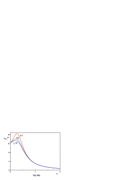
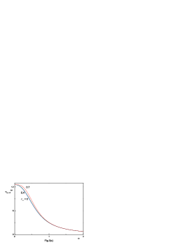
FIG. 2.: Plot of the partial absorption cross section for s-wave ($\ell=0$) when $r_{+}=1$ and $n=0$ (Fig. 2(a)), $r_{+}=1$ and $n=1$ (Fig. 2(b)), and $r_{+}=1$ and $n=2$ (Fig. 2(c)) with varying $r_{-}$. These figures show how the absorption cross section is enhanced with increasing $r_{-}$. Regardless of $n$ the low-energy absorption cross section equals to the horizon area $4\pi r_{+}^{2}$, which is an universal properties for the asymptotically flat and spherically symmetric black holes

Fig. 2 shows $r_{-}$-dependence of the partial absorption cross section for s-wave ($\ell=0$) when $n=0$, $1$ and $2$. As expected from the effective potential the absorption cross section is enhanced with increasing $r_{-}$. The sharp peaks in Fig. 2(a) ($n=0$ case) disappear in Fig. 2(c) ($n=2$ case). This seems to be because the presence of the extra dimensions strongly suppresses the absorptivity of the black hole, which is clear from Fig. 1(b) or Fig. 3. Regardless of $n$ the low-energy absorption cross section equals to $4\pi r_{+}^{2}$, which is an universal property for the asymptotically flat and spherically symmetric black holes[14].

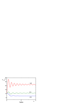
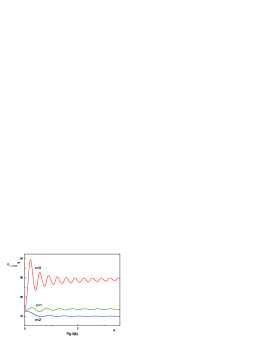
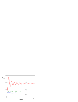
FIG. 3.: Plot of the total absorption cross section when $r_{+}=1$, and $r_{-}=0$ (Fig. 3(a)), $0.4$ (Fig. 3(b)), and 0.7 (Fig. 3(c)) with varying $n$. These figures show how the existence of the extra dimensions suppresses the absorption cross section. Regardless of $n$ and/or $r_{-}$ the low energy absorption cross section equals to the horizon area. This fact indicates that the higher partial waves ($\ell\geq 1$) have vanishing low-energy limits.

Fig. 3 shows the $n$-dependence of the total absorption cross section $\sigma_{T}^{BR}$ when $r_{-}=0$, $0.4$ and $0.7$. The oscillatory behavior of $\sigma_{T}^{BR}$ at $n=0$ indicates that each partial absorption cross section with different angular momentum $\ell$ has a peak in the different value of $\omega$. This oscillatory behavior, however, disappears with increase of $n$. This is because the presence of the extra dimensions removes the peak of the each partial absorption cross section as Fig. 2(c) exhibits. The fact that $\sigma_{T}^{BR}(\omega=0)=4\pi r_{+}^{2}$ indicates that the partial absorption cross sections for $\ell\geq 1$ vanish in the low-energy limit, which is in good agreement with Starobinsky’s formula[8].

From the Hawking formula (1) the brane emission, i.e. the energy emitted per unit time and energy interval $d\omega$, is given by

$$\Gamma_{D}^{BR}=\frac{\omega^{3}\sigma_{abs}}{2\pi^{2}\left(e^{\omega/T_{H}}-1\right)}d\omega$$ (69)

for the massless scalar localized on the brane. The effect of the extra dimensions is included in the absorption cross section $\sigma_{abs}$ and the Hawking temperature $T_{H}$. Since $\sigma_{abs}$ decreases and $T_{H}$ increases in the presence of the extra dimensions, the complete emission spectrum is determined by the competition between the greybody and Planck factors. Since, in addition, the inner horizon parameter $r_{-}$ generally increases $\sigma_{abs}$ and decreases $T_{H}$, the emission rate in the presence of nonzero $r_{-}$ is also determined by the competition between these two factor.

Since, in general, the effect of the Planck factor is dominant compared to the greybody factor in the emission problem, we expect that the presence of the extra dimensions enhances the emission spectrum. We also expect that contrary to the extra dimensions the presence of nonzero $r_{-}$ may decrease the emission spectrum of the black hole.

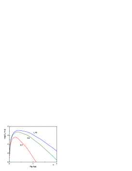
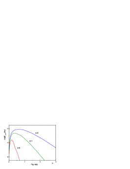
FIG. 4.: Log-plot of the emission rate when $r_{+}=1$ and $n=1$ with varying $r_{-}$ (Fig. 4(a)), and when $r_{+}=1$ and $r_{-}=0.4$ with varying $n$ (Fig. 4(b)). These figures shows the emission rate reduces with increasing $r_{-}$. However, the presence of the extra dimensions in general enhances the emission power. These facts indicate that the Planck factor is dominant compared to the greybody factor in the emission problem.

Fig. 4(a) is a $r_{-}$-dependence of the emission rate when $n=1$. As expected, the emission rate decreases with increase of $r_{-}$. As commented earlier the frozen black hole seems to have a poor ability in the emission. Contrary to the Wien’s type of displacement of the peak, the peak moves to the opposite direction with increasing $r_{-}$ in this figure. Fig. 4(b) is a $n$-dependence of the emission rate when $r_{-}=0.4$. As expected again, the existence of the extra dimensions enhances the emission rate.

IV wave equation for the bulk scalar

The scalar equation $(\Box-m^{2})\Phi_{BL}=0$ for the bulk scalar in the background of the spacetime (5) reduces to the following radial equation

$$x(x^{n+1}-x_{+}^{n+1})^{2}(x^{n+1}-x_{-}^{n+1})^{2}\frac{d^{2}R}{dx^{2}}+(x^{n+1}-x_{+}^{n+1})(x^{n+1}-x_{-}^{n+1})$$ (70)

$$\hskip 14.22636pt\times\left[(n+1)x^{n+1}(2x^{n+1}-x_{+}^{n+1}-x_{-}^{n+1})-n(x^{n+1}-x_{+}^{n+1})(x^{n+1}-x_{-}^{n+1})\right]\frac{dR}{dx}$$ (71)

$$\hskip 56.9055pt+\Bigg{[}x^{4n+5}-\ell(\ell+n+1)x^{2n+1}(x^{n+1}-x_{+}^{n+1})(x^{n+1}-x_{-}^{n+1})$$ (72)

$$\hskip 113.81102pt+\frac{m^{2}}{\omega^{2}v^{2}}x^{2n+3}\left\{x^{n+1}(x_{+}^{n+1}+x_{-}^{n+1})-x_{+}^{n+1}x_{-}^{n+1}\right\}\Bigg{]}R=0$$ (73)

where $x\equiv\omega vr$ and $x_{\pm}\equiv\omega vr_{\pm}$. Of course, we assumed the separability condition $\Phi_{BL}=e^{-i\omega t}R(r)\tilde{Y}(\Omega)$, where $\tilde{Y}$ is an higher-dimensional spherical harmonics. From now on we take the massless case ($m=0$) for simplicity.

From Eq.(70) it is straightforward to derive the following Schrödinger-like equation

$$-\frac{d^{2}\psi}{dr_{*}^{2}}+V_{eff}^{BL}\psi=\omega^{2}\psi$$ (74)

where the tortoise coordinate $r_{*}$ is given in Eq.(18) and $\psi=r^{(n+2)/2}R$. The effective potential $V_{eff}^{BL}$ is given by

$$V_{eff}^{BL}=\frac{h_{n}(r)}{r^{2}}\left[\ell(\ell+n+1)+\frac{n+2}{2}\left\{(n+1)(h_{n,+}(r)+h_{n,-}(r))-\frac{3n+4}{2}h_{n}(r)\right\}\right].$$ (75)

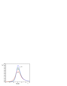
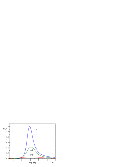
FIG. 5.: (a) Plot of the effective potential $V_{eff}^{BL}$ with respect to the tortoise coordinate $r_{*}$ for $r_{-}=0$, $0.4$ and $0.7$ when $n=1$, $\ell=0$ and $r_{+}=1$. This figure indicates the absorption cross section enhances with increase of $r_{-}$. This fact can be deduced also from the Hawking temperature. (b) Plot of the effective potential $V_{eff}^{BL}$ with respect to the tortoise coordinate $r_{*}$ for $n=0$, $1$ and $2$ when $r_{-}=0.4$, $r_{+}=1$ and $\ell=0$. This figure indicates that the absorptivity of black hole for the bulk scalar may be suppressed with increase of $n$.

Fig. 5 is a plot of $V_{eff}^{BL}$ with respect to the tortoise coordinate $r_{*}$. Since the $r_{*}$-dependence of $V_{eff}^{BL}$ is very similar to the $r_{*}$-dependence of $V_{eff}^{BR}$ in Fig. 1, the absorption spectrum seems to be enhanced with increasing $r_{-}$. Also Fig. 5(b) indicates that the absorptivity for the bulk scalar by a black hole may be suppressed with increase of $n$. As will be shown in the following section, however, the disappearance of the oscillatory pattern in the total absorption cross section occured in the case of the brane-localized scalar does not happen in this case although the amplitude of oscillation decreases in the presence of the extra dimensions.

The calculational procedure for the numerical computation of the absorption cross section for the bulk scalar in the full-range of energy is similar to that for the case of the brane-localized scalar. The Wronskian of $R$ and $R^{*}$ which are solutions of the radial equation (70) is

$$W[R^{*},R]_{x}\equiv R^{*}\frac{dR}{dx}-R\frac{dR^{*}}{dx}=\frac{C_{n}^{\prime}x^{n}}{(x^{n+1}-x_{+}^{n+1})(x^{n+1}-x_{-}^{n+1})}$$ (76)

where $C_{n}^{\prime}$ is a $n$-dependent integration constant. Comparing Eq.(76) with the corresponding equation (25) in the brane case, the only difference of the Wronskian is the power of $x$ in the numerator. However, this slight difference is crucial and makes completely different absorption and emission spectra from those for the case of the brane-localized scalar.

The solutions of the radial equation (70) which has a convergent range around the near-horizon region can be derived in the similar way to the brane-localized case

$${\cal G}_{n,\ell}(x,x_{+},x_{-})=e^{\lambda_{n}\ln|x-x_{+}|}\sum_{N=0}^{\infty}d_{\ell,N}(x-x_{+})^{N}$$ (77)

where $\lambda_{n}$ is given in Eq.(27). For $n=0$ the recursion relation which the coefficient $d_{\ell,N}$ obeys should be same with Eq.(28) because there is no distinction between the cases of bulk and brane. However, the recursion relations for $n\geq 1$ should be different from those in the brane-localized case. In appendix B the recursion relation of $d_{\ell,N}$ for $n=1$ is explicitly given. As in the case of the brane-localized scalar the recursion relations for $n\geq 2$ are not presented in the paper because they are too lengthy.

The solutions of Eq.(70) which are convergent in the asymptotic region can be expressed as[6]

$${\cal F}_{n,\ell(\pm)}(x,x_{+},x_{-})=(\pm i)^{\ell+1+\frac{n}{2}}\frac{e^{\mp ix}(x-x_{+})^{\pm\lambda_{n}}}{x^{\frac{n}{2}}}\sum_{N=0}^{\infty}\tau_{N(\pm)}x^{-(N+1)}$$ (78)

where ${\cal F}_{n,\ell(+)}$ and ${\cal F}_{n,\ell(-)}$ are ingoing and outgoing solutions respectively. The difference of Eq.(78) from Eq.(31) is a power of $x$ in the denominator, which is also crucial in the following calculation. As remaked just before, the recursion relation of $\tau_{N(\pm)}$ for $n=0$ should be same with Eq.(32). The recursion relation for $n=1$ is explicitly given in appendix B. Using Eq.(76) it is easy to show

$$W[{\cal G}_{n,\ell}^{*},{\cal G}_{n,\ell}]_{x}\equiv{\cal G}_{n,\ell}^{*}\partial_{x}{\cal G}_{n,\ell}-{\cal G}_{n,\ell}\partial_{x}{\cal G}_{n,\ell}^{*}=\frac{-2i|g_{n,\ell}|^{2}x_{+}^{n+2}x^{n}}{(x^{n+1}-x_{+}^{n+1})(x^{n+1}-x_{-}^{n+1})}$$ (79)

$$W[{\cal F}_{n,\ell(+)},{\cal F}_{n,\ell(-)}]_{x}\equiv{\cal F}_{n,\ell(+)}\partial_{x}{\cal F}_{n,\ell(-)}-{\cal F}_{n,\ell(-)}\partial_{x}{\cal F}_{n,\ell(+)}=\frac{2ix^{n}}{(x^{n+1}-x_{+}^{n+1})(x^{n+1}-x_{-}^{n+1})}$$ (80)

where $g_{n,\ell}\equiv d_{\ell,0}$.

The equation for the bulk scalar case corresponding to Eq(44) for the brane-localized case is[6]

$$R_{n,\ell}\stackrel{{\scriptstyle x\rightarrow x_{+}}}{{\sim}}g_{n,\ell}(x-x_{+})^{\lambda_{n}}\left[1+O(x-x_{+})\right]$$ (81)

$$R_{n,\ell}\stackrel{{\scriptstyle x\rightarrow\infty}}{{\sim}}\frac{i^{\ell+1+\frac{n}{2}}2^{\frac{n}{2}-1}}{\sqrt{\pi}x^{1+\frac{n}{2}}}\Gamma{(\frac{1+n}{2})}\frac{(2\ell+1+n)(\ell+n)!}{\ell!n!}$$ (82)

$$\hskip 51.21504pt\times\bigg{[}e^{-ix+\lambda_{n}\ln|x-x_{+}|}-(-1)^{\ell+\frac{n}{2}}S_{n,\ell}(x_{+},x_{-})e^{ix+\lambda_{n}\ln|x-x_{+}|}\bigg{]}+O\left(\frac{1}{x^{2+\frac{n}{2}}}\right)$$ (83)

where $R_{n,\ell}$ is a real scattering solution of Eq.(70) and $S_{n,\ell}$ is a partial scattering amplitude. If we define a phase shift $\delta_{n,\ell}$ as $S_{n,\ell}\equiv e^{2i\delta_{n,\ell}}$, the second equation of Eq.(81) can be written as

$$R_{n,\ell}\stackrel{{\scriptstyle x\rightarrow\infty}}{{\sim}} \frac{2^{\frac{n}{2}}}{\sqrt{\pi}x^{1+\frac{n}{2}}}\Gamma{(\frac{1+n}{2})}\frac{(2\ell+1+n)(\ell+n)!}{\ell!n!}e^{i\delta_{n,\ell}}$$ (85)

$$\times\sin\left[x+i\lambda_{n}\ln|x-x_{+}|-\frac{\pi}{2}(\ell+\frac{n}{2})+\delta_{n,\ell}\right]+O\left(\frac{1}{x^{2+\frac{n}{2}}}\right).$$

Following the same way of section II the Wronskian $W[R_{n,\ell}^{*},R_{n,\ell}]_{x}$ becomes in the form

$$W[R_{n,\ell}^{*},R_{n,\ell}]_{x} = -i\frac{2^{n}}{\pi}\Gamma^{2}{(\frac{1+n}{2})}\left(\frac{(2\ell+1+n)(\ell+n)!}{\ell!n!}\right)^{2}$$ (86)

$$\times \frac{x^{n}e^{-2\beta_{n,\ell}}}{(x^{n+1}-x_{+}^{n+1})(x^{n+1}-x_{-}^{n+1})}\sinh{2\beta_{n,\ell}}$$ (87)

where we assumed $\delta_{n,\ell}$ is a complex quantity, i.e. $\delta_{n,\ell}\equiv\eta_{n,\ell}+i\beta_{n,\ell}$. Since $R_{n,\ell}$ and ${\cal G}_{n,\ell}$ exhibit a same behavior around the near-horizon region, $W[R_{n,\ell}^{*},R_{n,\ell}]_{x}$ should be same with $W[{\cal G}_{n,\ell}^{*},{\cal G}_{n,\ell}]_{x}$, which is given in Eq.(79). Equating those two Wronskians yield a relation.

$$|g_{n,\ell}|^{2}=\frac{2^{n-2}}{\pi x_{+}^{n+2}}\Gamma^{2}{(\frac{1+n}{2})}\left(\frac{(2\ell+1+n)(\ell+n)!}{\ell!n!}\right)^{2}(1-e^{-4\beta_{n,\ell}})$$ (88)

As in the same way with section II we introduce $\tilde{R}_{n,\ell}(x,x_{+},x_{-})$, which is different from $R_{n,\ell}(x,x_{+},x_{-})$ in its normalization in such a way that

$$\tilde{R}_{n,\ell}(x,x_{+},x_{-})\stackrel{{\scriptstyle x\rightarrow x_{+}}}{{\sim}}(x-x_{+})^{\lambda_{n}}\left[1+O(x-x_{+})\right].$$ (89)

Expressing $\tilde{R}_{n,\ell}$ in terms of the jost functions

$$\tilde{R}_{n,\ell}(x,x_{+},x_{-})=f_{n,\ell}^{(-)}(x_{+},x_{-}){\cal F}_{n,\ell(+)}(x,x_{+},x_{-})+f_{n,\ell}^{(+)}(x_{+},x_{-}){\cal F}_{n,\ell(-)}(x,x_{+},x_{-}),$$ (90)

one can show easily that the jost functions $f_{n,\ell}^{(\pm)}$ are obtained by

$$f_{n,\ell}^{(\pm)}(x_{+},x_{-}) = \pm\frac{(x^{n+1}-x_{+}^{n+1})(x^{n+1}-x_{-}^{n+1})}{2ix^{n}}W[{\cal F}_{n,\ell(\pm)},\tilde{R}]_{x}$$ (91)

$$= \pm\frac{\omega^{n+1}(r^{n+1}-r_{+}^{n+1})(r^{n+1}-r_{-}^{n+1})}{2ir^{n}}W[{\cal F}_{n,\ell(\pm)},\tilde{R}]_{r}.$$ (92)

Inserting the explicit from of ${\cal F}_{n,\ell(\pm)}$ into Eq.(90) and comparing it with Eq.(81), one can derive the relations

$$S_{n,\ell}(x_{+},x_{-}) = \frac{f_{n,\ell}^{(+)}(x_{+},x_{-})}{f_{n,\ell}^{(-)}(x_{+},x_{-})}$$ (93)

$$f_{n,\ell}^{(-)}(x_{+},x_{-}) = \frac{2^{\frac{n}{2}-1}}{\sqrt{\pi}g_{n,\ell}(x_{+},x_{-})}\Gamma{(\frac{1+n}{2})}\frac{(2\ell+1+n)(\ell+n)!}{\ell!n!}.$$ (94)

Combining Eq.(88) and (93) enables us to express the greybody factor in terms of the jost function

$$1-|S_{n,\ell}(x_{+},x_{-})|^{2}=\frac{x_{+}^{n+2}}{|f_{n,\ell}^{(-)}(x_{+},x_{-})|^{2}}.$$ (95)

Thus making use of Eq.(3) with replacing ${\cal T}_{\ell}(\omega)$ by $1-|S_{n,\ell}(x_{+},x_{-})|^{2}$, the absorption cross section for the bulk scalar is expressed in the form

$$\sigma_{n,\ell}^{BL}=2^{n+1}\pi^{\frac{n+1}{2}}\Gamma{(\frac{n+3}{2})}\frac{(2\ell+n+1)(\ell+n)!}{(n+1)!\ell!}\frac{r_{+}^{n+2}}{|f_{n,\ell}^{(-)}|^{2}}.$$ (96)

Therefore we can compute the absorption spectrum completely if the jost function $f_{n,\ell}^{(-)}$ is computed. Once the absorption cross section is known, the emission spectrum is also computed with an aid of the Hawking formula (1).

V Absorption and Emission for the bulk scalar

In this section we will compute the jost functions $f_{n,\ell}^{(\pm)}(x_{+},x_{-})$ introduced in section IV (see Eq.(90)) numerically. Following the same way of section III we firstly derive a solution $\varphi_{n,\ell}(x,x_{+},x_{-})$ of the radial equation (70), which has a convergent range in the neighborhood of an arbitrary point $x=b$. Of course this solution is expressed as a power series in the form

$$\varphi_{n,\ell}(x,x_{+},x_{-})=(x-x_{+})^{\lambda_{n}}\sum_{N=0}^{\infty}D_{N}(x-b)^{N}.$$ (97)

Of course, when $n=0$, the recursion relation of $D_{N}$ is exactly same with Eq.(58) because there is no distinction between brane and bulk. The recursion relation for $n=1$ is given explicitly in appendix B. Then, as explained in section II, it is possible to compute the jost functions via the analytic continuation.

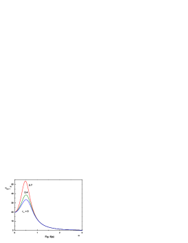
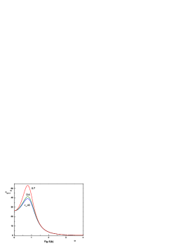
FIG. 6.: Plot of the partial absorption cross section for s-wave ($\ell=0$) for $n=r_{+}=1$ (Fig. 6(a)) and $n=2r_{+}=2$ (Fig. 6(b)) with varying $r_{-}$. Plot for $n=0$ is same with Fig. 2(a). These figures show how the absorption cross section is enhanced with increasing $r_{-}$. Regardless of $r_{-}$, the low-energy cross sections exactly equal to the area of the horizon hypersurface.

Fig. 6 shows $r_{-}$-dependence of the partial absorption cross section for $s$-wave ($\ell=0$) when $n=1$ (Fig. 6(a)) and $n=2$ (Fig. 6(b)). For the case of $n=0$ Fig. 2(a) should be reproduced as remarked earlier. Like a brane-localized case increasing $r_{-}$ enhances the absorption cross section, which can be understood from the Hawking temperature (7). Unlike a brane-localized case, however, the low-energy absorption cross sections are $2\pi^{2}r_{+}^{3}$ for $n=1$ and $8\pi^{2}r_{+}^{4}/3$ for $n=2$, which coincide with the area of the horizon hypersurfaces. While sharp peak disappears in Fig. 2 for large $n$, this property is not maintained in the bulk absorption problem.

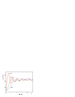
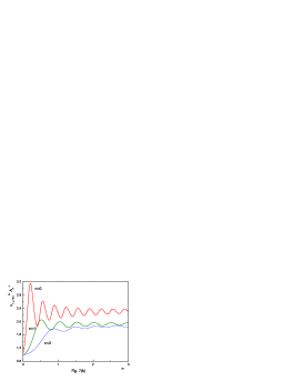
FIG. 7.: Plot of $\sigma_{T}^{BL}/A_{H}$ when $r_{+}=1$, and $r_{-}=0$ (Fig. 7(a)), $r_{-}=0.4$ (Fig. 7(b)) and $r_{-}=0.7$ (Fig. 7(c)) with varying $n$. Unlike Fig. 3 the oscillatory pattern does not disappear in the presence of nonzero $n$. For nonzero $n$ the total absorption cross section tends to be inclined with positive slope. This slope seems to increase with increasing $n$.

Fig. 7 shows the $n$-dependence of $\sigma_{T}^{BL}/A_{H}$ when $r_{-}=0$ (Fig. 7(a)), $0.4$ (Fig. 7(b)) and $0.7$ (Fig. 7(c)) where $\sigma_{T}^{BL}$ and $A_{H}$ are total absorption cross section and the horizon area, respectively. Unlike Fig. 3 for the brane-localized case the oscillatory behavior does not disappear regardless of $n$ in spite of the decrease of the oscillation amplitude. This fact indicates that the presence of the extra dimensions does not strongly suppress the absorptivity, which can be understood from Fig. 6. A remarkable fact appearing in Fig. 7 is that the total absorption cross section tends to be inclined with a positive slope in the course of oscillation when the extra dimensions exist. The slope seems to increase with increasing $n$. Similar behavior was found in the absorption of the dilaton-axion by an extremal D3-brane [46].

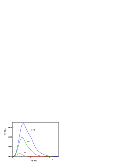
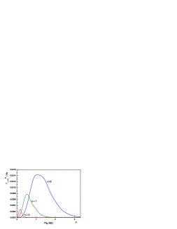
FIG. 8.: Plot of the emission rate when $r_{+}=n=1$ with varying $r_{-}$ (Fig. 8(a)), and when $r_{+}=1$ and $r_{-}=0.4$ with varying $n$ (Fig. 4(b)). Fig. 8(a) indicates that the emission rate is suppressed with increasing $r_{-}$. The presence of the extra dimensions generally enhances the emission rate as Fig. 8(b) indicates. These facts imply that the Planck factor is a dominant factor in the emission spectrum.

Finally let us discuss the emission problem for the bulk scalar. The Hawking formula (1) makes the bulk emission, i.e. the energy emitted to the bulk per unit time and energy interval $d\omega$ to be

$$\Gamma_{D}^{BL}=\left(2^{D-2}\pi^{\frac{D-1}{2}}\Gamma{(\frac{D-1}{2})}\right)^{-1}\frac{\omega^{D-1}\sigma_{abs}(\omega)}{e^{\frac{\omega}{T_{H}}}-1}d\omega$$ (98)

where $D$ is a spacetime dimensions. Since $T_{H}$ decreases with increasing of $r_{-}$, it is evident that the emission rate drastically decreases with increase of $r_{-}$. This is confirmed in Fig. 8(a) where $D$ and $r_{+}$ are fixed as $r_{+}=1$ and $D=5$. Since, in addition, $T_{H}$ increases in the presence of the extra dimensions, the emission rate should be enhanced with increasing $n$. This fact is also confirmed in Fig. 8(b), where $r_{+}$ and $r_{-}$ are fixed as $r_{+}=1$ and $r_{-}=0.4$.

VI Bulk versus Brane

In this section we would like to compare the emission spectra for the brane-localized and the bulk scalars, which was a main issue in Ref.[45, 47, 48]. From Eq.(69) and Eq.(98) the ratio of the emission spectra is

$$\gamma_{D}(\omega)\equiv\frac{\Gamma_{D}^{BL}/d\omega}{\Gamma_{D}^{BR}/d\omega}=\frac{\pi^{\frac{5-D}{2}}\omega^{D-4}}{2^{D-3}\Gamma\left(\frac{D-1}{2}\right)}\frac{\sigma_{T}^{BL}}{\sigma_{T}^{BR}}.$$ (99)

As expected $\gamma_{4}=1$ when $D=4$ due to $\sigma_{T}^{BL}=\sigma_{T}^{BR}$ when $n=0$. When $D=5$ and $6$, this ratio factor becomes

$$\gamma_{5}(\omega)=\frac{\omega}{4}\frac{\sigma_{T}^{BL}}{\sigma_{T}^{BR}}\hskip 56.9055pt\gamma_{6}(\omega)=\frac{\omega^{2}}{6\pi}\frac{\sigma_{T}^{BL}}{\sigma_{T}^{BR}}.$$ (100)

Thus in the low-energy region ($\omega<<1$) $\gamma_{5}\sim\pi r_{+}\omega/8\sim 0$ and $\gamma_{6}\sim r_{+}^{2}\omega^{2}/9\sim 0$. Thus in this region the emission into the brane is dominant compared to the emission into the bulk.

In the high-energy region ($\omega>>1$), however, the emission into the bulk becomes larger than that into the brane due to $\omega$ factor in Eq.(99).

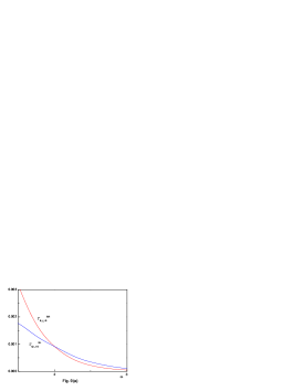
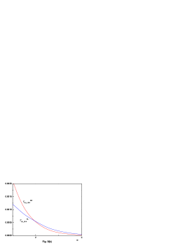
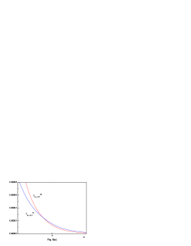
FIG. 9.: Plot of the emission rate for the bulk and brane-localized scalars at $D=6$ in the neighborhood of $\omega_{\ast}$, where $\Gamma_{6}^{BR}(\omega_{\ast})=\Gamma_{6}^{BL}(\omega_{\ast})$, when $r_{-}=0$ (Fig. 9(a)), $r_{-}=0.4$ (Fig. 9(b)) and $r_{-}=0.7$ (Fig. 9(c)). These figures show that $\Gamma_{6}^{BR}>\Gamma_{6}^{BL}$ when $\omega<\omega_{\ast}$ and $\Gamma_{6}^{BR}<\Gamma_{6}^{BL}$ when $\omega>\omega_{\ast}$. This fact indicates that the emission into the brane is dominant in the domain of low-energy and the emission into bulk is dominant in the domain of high-energy.

The low-energy and high-energy behavior of $\gamma_{D}(\omega)$ are confirmed in Fig. 9, where the emission spectra for the bulk and the brane-localized scalars are plotted simultaneously for $r_{-}=0$ (Fig. 9(a)), $r_{-}=0.4$ (Fig. 9(b)) and $r_{-}=0.7$ (Fig. 9(c)) when $D=6$. These figures are plotted in the neighborhood of a point where $\Gamma_{6}^{BR}$ and $\Gamma_{6}^{BL}$ coincide with each other. These figures shows that $\Gamma_{6}^{BL}-\Gamma_{6}^{BR}$ in the high-energy domain decreases with increasing $r_{-}$. This means the ratio of the total emission rate $\Gamma_{D}^{BL}/\Gamma_{D}^{BR}$ decreases with increasing $r_{-}$.

To confirm this fact we computed $\Gamma_{D}^{BL}$, $\Gamma_{D}^{BR}$ and their ratio for $r_{-}=0$, $r_{-}=0.4$, and $r_{-}=0.7$ when $n=0$ (Table 1), $n=1$ (Table 2), and $n=2$ (Table 3).

Table1: Comparision of bulk to brane emission in $n=0$

	$r_{-}=0$	$r_{-}=0.4$	$r_{-}=0.7$
$\Gamma_{4}^{BR}$	$0.000297531$	$0.0000522908$	$3.30229\times 10^{-6}$
$\Gamma_{4}^{BL}$	$0.000297531$	$0.0000522908$	$3.30229\times 10^{-6}$
$\Gamma_{4}^{BL}/\Gamma_{4}^{BR}$	$1$	$1$	$1$

Table2: Comparision of bulk to brane emission in $n=1$

	$r_{-}=0$	$r_{-}=0.4$	$r_{-}=0.7$
$\Gamma_{5}^{BR}$	$0.00266319$	$0.00141917$	$0.000223692$
$\Gamma_{5}^{BL}$	$0.00104967$	$0.000488455$	$0.0000478151$
$\Gamma_{5}^{BL}/\Gamma_{5}^{BR}$	$0.394$	$0.344183$	$0.213754$

Table3: Comparision of bulk to brane emission in $n=2$

	$r_{-}=0$	$r_{-}=0.4$	$r_{-}=0.7$
$\Gamma_{6}^{BR}$	$0.0107479$	$0.00841889$	$0.00224066$
$\Gamma_{6}^{BL}$	$0.00267917$	$0.00187831$	$0.000263698$
$\Gamma_{6}^{BL}/\Gamma_{6}^{BR}$	$0.249274$	$0.223107$	$0.117688$

These Tables indicate that the emission into the brane is dominant compared to emission into the bulk regardless of $r_{-}$ in the presence of extra dimensions, which is a main result of Ref.[45]. The ratio factor $\Gamma_{D}^{BL}/\Gamma_{D}^{BR}$ decreases with increasing $r_{-}$ as expected. Although the calculation is not explicitly carried out in this paper, the emission into bulk might be dominant compared to the emission into brane if our universe has sufficiently many extra dimensions. This is conjectured from the fact that the dominance of bulk emission in the high-energy domain can overwhelm the dominance of brane emission in the low-energy domain if $n$ is a sufficiently large due to the factor $\omega^{D-4}$ in Eq.(99).

Although our numerical computation supports the main claim of Ref.[45], i.e. black holes radiate mainly on the brane, there are several issues to consider seriously before we arrive at a conclusion for the dominant emissivity. Firstly, one should note that our computation presented in the Tables is restricted to the relative emission for the spin-$0$ field. Since the emission is in general highly dependent on the field spin, our result does not derive any conclusion to the dominant one between emission on the brane and off the brane when fields have higher spin. The emission for the higher spin particles manifestly need another detailed calculation.

Secondly, we have not considered in this paper the rotating effect of the black holes. Since the black holes produced by high-energy scattering are expected to be highly rotating due to non-zero impact parameter, it is very important to consider this effect. It is well-known that there exist the superradiance modes[49, 50] in the general relativistic rotating black holes, which means the amplification of the amplitude of the incident wave by making use of the energy extracted from a black hole. Recently, the existence of the superradiance modes in the brane world black holes has been shown analytically[51] and numerically[52, 53]. Also importance of the superradiance for the experimental signature in the colliders is stressed in Ref.[54, 55]. In Ref.[51] the existence of the superradiance for the bulk scalars incident on five-dimensional rotating black holes is proved analytically. In Ref.[52, 53] the effect of the superradiance for the brane-localized scalars has been studied numerically at $D=10$ and $D=6$, respectively. Since the effect of the superradiance is not taken into account in Ref.[45] and present paper, the debate on the dominant emissivity is not finished yet.

VII Conclusion

In this paper we examined the absorption and emission spectra for the brane-localized and bulk scalars when the spacetime is a ($4+n$)-dimensional RN black hole. In particular, the effects of the inner horizon parameter $r_{-}$ and the number of toroidally compactified extra dimensions $n$ are rigorously discussed throughout the paper. For calculational technique we adopt the numerical calculation introduced in Ref[13, 20, 21] for the computation of the absorption and emission spectra in the full-range of energy of the scalar particles.

For the case of the brane-localized scalar it turns out that the presence of $r_{-}$ generally enhances the absorptivity compared to the case of the Schwarzschild phase. This can be deduced from a fact that the Hawking temperature given in Eq.(7) decreases with increasing $r_{-}$. The low-energy absorption cross section exactly equals to $4\pi r_{+}^{2}$, which is an universality for the spherically symmetric and asymptotically flat black holes. The emission is generally reduced with increasing $r_{-}$, which indicates the the Planck factor is more dominant than the greybody factor in the emission problem. The presence of the extra dimensions suppresses the absorption spectrum and enhances the emission spectrum compared to those without the extra dimension. Especially, the oscillatory pattern of the total absorption cross section disappears when $n$ is large. The reason for this might be the fact that the suppression of the absorptivity in the presence of the extra dimensions is too strong.

For the case of the bulk scalar the effects of $r_{-}$ and $n$ in the absorption and emission spectra are similar to the case of the brane-localized scalar. Unlike the brane-localized case, however, the disappearance of the oscillatory pattern in the total absorption cross section does not manifestly happen in this case although the amplitude of oscillation decreases with increasing $n$. This means the presence of the extra dimensions does not suppress the absorptivity too much strongly. The total absorption cross section tends to be inclined with a positive slope when the extra dimensions exist. This slope seems to increase with increasing $n$. The low-energy absorption cross section is not dependent on $r_{-}$ and equals to the area of the horizon hypersurface, which is also universality for the spherically symmetric and asymptotically flat black holes.

Finally, we discussed the ratio of the brane emission to the bulk emission. It turns out that the brane emission is dominant in the low-energy domain while the bulk emission is larger than the brane emission in the high-energy domain. For comparatively small $n$ the total emission rate into the brane is much larger than that into the bulk. If, however, $n$ is sufficiently large, the bulk emission can be dominant because of $\omega$-dependent factor in Eq.(99). Our numerical calculation shows that the ratio factor $\Gamma_{D}^{BL}/\Gamma_{D}^{BR}$ decreases with increasing $r_{-}$.

It is interesting to extend our paper to the particles with spin. This is important when $n$ is large because the emission rate for the particles with higher spin is dominant in the higher-dimensional theories. We may use a Newman-Penrose formalism[56, 57] to derive a master equation. It is interesting to discuss the effect of the inner horizon parameter $r_{-}$ in the absorption and emission problems for the particles with spin.

Although this paper is strongly motivated by the recent brane-world scenarios, our computational techniques can be directly applied to the five-dimensional RN black hole carrying three different electric charges and the corresponding six-dimensional black string introduced in Ref.[27, 29] for the computation of the absorption and emission spectra in the full-range of energy. This calculation may give interesting results in the correspondence between the black hole and D-brane beyond the dilute gas region.

It is also important to extend our calculation to the rotating effect of black holes. Especially, as claimed in Ref.[51, 54, 55] the effect of the superradiance should be examined carefully to determine the dominant one between bulk and brane emission. Work on this issue is in progress and will be reported elsewhere.

Acknowledgement: This work was supported by the Kyungnam University Research Fund, 2004.

Appendix A

The recursion relation for $n=1$ which is correspondent to Eq.(28) for $n=0$ is

$$\left[(N+\lambda_{1})(N+\lambda_{1}-1)\alpha_{1}+(N+\lambda_{1})\beta_{1}+\gamma_{1}\right]d_{\ell,N}$$ (A.1)

$$+ \left[(N+\lambda_{1}-1)(N+\lambda_{1}-2)\alpha_{2}+(N+\lambda_{1}-1)\beta_{2}+\gamma_{2}\right]d_{\ell,N-1}$$ (A.2)

$$+ \left[(N+\lambda_{1}-2)(N+\lambda_{1}-3)\alpha_{3}+(N+\lambda_{1}-2)\beta_{3}+\gamma_{3}\right]d_{\ell,N-2}$$ (A.3)

$$+ \left[(N+\lambda_{1}-3)(N+\lambda_{1}-4)\alpha_{4}+(N+\lambda_{1}-3)\beta_{4}+\gamma_{4}\right]d_{\ell,N-3}$$ (A.4)

$$+ \left[(N+\lambda_{1}-4)(N+\lambda_{1}-5)\alpha_{5}+(N+\lambda_{1}-4)\beta_{5}+\gamma_{5}\right]d_{\ell,N-4}$$ (A.5)

$$+ \left[(N+\lambda_{1}-5)(N+\lambda_{1}-6)\alpha_{6}+(N+\lambda_{1}-5)\beta_{6}+\gamma_{6}\right]d_{\ell,N-5}$$ (A.6)

$$+ \left[(N+\lambda_{1}-6)(N+\lambda_{1}-7)\alpha_{7}+(N+\lambda_{1}-6)\beta_{7}+\gamma_{7}\right]d_{\ell,N-6}$$ (A.7)

$$+ \left[(N+\lambda_{1}-7)(N+\lambda_{1}-8)+2(N+\lambda_{1}-7)+\gamma_{8}\right]d_{\ell,N-7}+\gamma_{9}d_{\ell,N-8}+d_{\ell,N-9}=0$$ (A.8)

where

$$\alpha_{1}=4x_{+}^{3}(x_{+}^{2}-x_{-}^{2})^{2}\hskip 91.04872pt\alpha_{2}=8x_{+}^{2}(x_{+}^{2}-x_{-}^{2})(3x_{+}^{2}-x_{-}^{2})$$ (A.9)

$$\alpha_{3}=x_{+}(61x_{+}^{4}-50x_{+}^{2}x_{-}^{2}+5x_{-}^{4})\hskip 28.45274pt\alpha_{4}=85x_{+}^{4}-38x_{+}^{2}x_{-}^{2}+x_{-}^{4}$$ (A.10)

$$\alpha_{5}=14x_{+}(5x_{+}^{2}-x_{-}^{2})\hskip 65.44142pt\alpha_{6}=2(17x_{+}^{2}-x_{-}^{2})\hskip 28.45274pt\alpha_{7}=9x_{+}$$ (A.11)

$$\beta_{1}=4x_{+}^{3}(x_{+}^{2}-x_{-}^{2})^{2}\hskip 71.13188pt\beta_{2}=2x_{+}^{2}(x_{+}^{2}-x_{-}^{2})(13x_{+}^{2}-x_{-}^{2})$$ (A.12)

$$\beta_{3}=8x_{+}^{3}(9x_{+}^{2}-5x_{-}^{2})\hskip 65.44142pt\beta_{4}=10x_{+}^{2}(11x_{+}^{2}-3x_{-}^{2})$$ (A.13)

$$\beta_{5}=4x_{+}(25x_{+}^{2}-3x_{-}^{2})\hskip 65.44142pt\beta_{6}=2(27x_{+}^{2}-x_{-}^{2})\hskip 28.45274pt\beta_{7}=16x_{+}$$ (A.14)

$$\gamma_{1}=x_{+}^{9}\hskip 142.26378pt\gamma_{2}=x_{+}^{4}\left[9x_{+}^{4}-2\ell(\ell+1)(x_{+}^{2}-x_{-}^{2})\right]\hskip 28.45274pt$$ (A.15)

$$\gamma_{3}=x_{+}^{3}\left[36x_{+}^{4}-\ell(\ell+1)(11x_{+}^{2}-7x_{-}^{2})\right]\hskip 28.45274pt\gamma_{4}=x_{+}^{2}\left[84x_{+}^{4}-\ell(\ell+1)(25x_{+}^{2}-9x_{-}^{2})\right]$$ (A.16)

$$\gamma_{5}=x_{+}\left[126x_{+}^{4}-5\ell(\ell+1)(6x_{+}^{2}-x_{-}^{2})\right]\hskip 28.45274pt\gamma_{6}=126x_{+}^{4}-\ell(\ell+1)(20x_{+}^{2}-x_{-}^{2})$$ (A.17)

$$\gamma_{7}=7x_{+}\left[12x_{+}^{2}-\ell(\ell+1)\right]\hskip 28.45274pt\gamma_{8}=36x_{+}^{2}-\ell(\ell+1)\hskip 28.45274pt\gamma_{9}=9x_{+}.$$ (A.18)

The recursion relation for $n=1$ which is correspondent to Eq.(32) is

$$\tau_{N(-)}[-(N+1)\tilde{\beta}_{1}+\tilde{\gamma}_{1}]+\tau_{N-1(-)}[N(N+1)-N\tilde{\beta}_{2}+\tilde{\gamma}_{2}]$$ (A.19)

$$+\tau_{N-2(-)}[-(N-1)\tilde{\beta}_{3}+\tilde{\gamma}_{3}]+\tau_{N-3(-)}[(N-2)(N-1)\tilde{\alpha}_{1}-(N-2)\tilde{\beta}_{4}+\tilde{\gamma}_{4}]$$ (A.20)

$$+\tau_{N-4(-)}[-(N-3)\tilde{\beta}_{5}+\tilde{\gamma}_{5}]+\tau_{N-5(-)}[(N-4)(N-3)\tilde{\alpha}_{2}-(N-4)\tilde{\beta}_{6}+\tilde{\gamma}_{6}]$$ (A.21)

$$+\tau_{N-6(-)}[-(N-5)\tilde{\beta}_{7}+\tilde{\gamma}_{7}]+\tau_{N-7(-)}[(N-6)(N-5)\tilde{\alpha}_{3}-(N-6)\tilde{\beta}_{8}+\tilde{\gamma}_{8}]$$ (A.22)

$$+\tau_{N-8(-)}[-(N-7)\tilde{\beta}_{9}+\tilde{\gamma}_{9}]+\tau_{N-9(-)}[(N-8)(N-7)\tilde{\alpha}_{4}-(N-8)\tilde{\beta}_{10}]=0$$ (A.23)

where $\tau_{0(-)}=1$, $\tau_{N(+)}=\tau_{N(-)}^{*}$ and

$$\tilde{\alpha}_{1}=-2(x_{+}^{2}+x_{-}^{2})\hskip 142.26378pt\tilde{\alpha}_{2}=x_{+}^{4}+4x_{+}^{2}x_{-}^{2}+x_{-}^{4}$$ (A.24)

$$\tilde{\alpha}_{3}=-2x_{+}^{2}x_{-}^{2}(x_{+}^{2}+x_{-}^{2})\hskip 113.81102pt\tilde{\alpha}_{4}=x_{+}^{4}x_{-}^{4}$$ (A.25)

$$\tilde{\beta}_{1}=2i\hskip 56.9055pt\tilde{\beta}_{2}=2(1-\lambda_{1})\hskip 56.9055pt\tilde{\beta}_{3}=-2[\lambda_{1}x_{+}+2i(x_{+}^{2}+x_{-}^{2})]$$ (A.26)

$$\tilde{\beta}_{4}=-2[(x_{+}^{2}+x_{-}^{2})-\lambda_{1}(x_{+}^{2}+2x_{-}^{2})]\hskip 28.45274pt\tilde{\beta}_{5}=2i[(x_{+}^{4}+x_{-}^{4})+4x_{+}^{2}x_{-}^{2}]+2\lambda_{1}x_{+}(x_{+}^{2}+2x_{-}^{2})$$ (A.27)

$$\tilde{\beta}_{6}=-2\lambda_{1}x_{-}^{2}(2x_{+}^{2}+x_{-}^{2})\hskip 71.13188pt\tilde{\beta}_{7}=-2x_{+}x_{-}^{2}[2ix_{+}(x_{+}^{2}+x_{-}^{2})+\lambda_{1}(2x_{+}^{2}+x_{-}^{2})]$$ (A.28)

$$\tilde{\beta}_{8}=2x_{+}^{2}x_{-}^{2}[x_{+}^{2}+(1+\lambda_{1})x_{-}^{2}]\hskip 42.67912pt\tilde{\beta}_{9}=2x_{+}^{3}x_{-}^{4}[ix_{+}+\lambda_{1}]\hskip 42.67912pt\tilde{\beta}_{10}=-2x_{+}^{4}x_{-}^{4}$$ (A.29)

$$\tilde{\gamma}_{1}=2i(1-\lambda_{1})\hskip 99.58464pt\tilde{\gamma}_{2}=2(x_{+}^{2}+x_{-}^{2})-\ell(\ell+1)-\lambda_{1}(1-\lambda_{1})-2i\lambda_{1}x_{+}$$ (A.30)

$$\tilde{\gamma}_{3}=-2i[(x_{+}^{2}+x_{-}^{2})-\lambda_{1}(x_{+}^{2}+2x_{-}^{2})+i\lambda_{1}^{2}x_{+}]$$ (A.31)

$$\tilde{\gamma}_{4}=-(x_{+}^{4}+x_{-}^{4})-4x_{+}^{2}x_{-}^{2}+\ell(\ell+1)(x_{+}^{2}+x_{-}^{2})+\lambda_{1}^{2}(x_{+}^{2}-2x_{-}^{2})+\lambda_{1}x_{+}[2i(x_{+}^{2}+2x_{-}^{2})+x_{+}]$$ (A.32)

$$\tilde{\gamma}_{5}=-2\lambda_{1}x_{-}^{2}[i(2x_{+}^{2}+x_{-}^{2})+2\lambda_{1}x_{+}+x_{+}]$$ (A.33)

$$\tilde{\gamma}_{6}=\left\{x_{+}^{2}[2(x_{+}^{2}+x_{-}^{2})-\ell(\ell+1)]-\lambda_{1}^{2}(2x_{+}^{2}-x_{-}^{2})-\lambda_{1}[2ix_{+}(2x_{+}^{2}+x_{-}^{2})-x_{-}^{2}]\right\}x_{-}^{2}$$ (A.34)

$$\tilde{\gamma}_{7}=2x_{+}x_{-}^{2}(\lambda_{1}+ix_{+})[(x_{+}^{2}+x_{-}^{2})+\lambda_{1}x_{-}^{2}]\hskip 28.45274pt\tilde{\gamma}_{8}=-x_{+}^{2}x_{-}^{4}[x_{+}^{2}-\lambda_{1}^{2}+\lambda_{1}(1-2ix_{+})]$$ (A.35)

$$\tilde{\gamma}_{9}=-2x_{+}^{3}x_{-}^{4}(\lambda_{1}+ix_{+})$$ (A.36)

The recursion relation for $n=1$ corresponding to Eq.(58) for $n=0$ is

$$D_{N}[N(N-1)\bar{\alpha}_{9}]+D_{N-1}[(N-1)(N-2)\bar{\alpha}_{8}+(N-1)\bar{\beta}_{9}]$$ (A.37)

$$+ D_{N-2}[(N-2)(N-3)\bar{\alpha}_{7}+(N-2)\bar{\beta}_{8}+\bar{\gamma}_{9}]+D_{N-3}[(N-3)(N-4)\bar{\alpha}_{6}+(N-3)\bar{\beta}_{7}+\bar{\gamma}_{8}]$$ (A.38)

$$+ D_{N-4}[(N-4)(N-5)\bar{\alpha}_{5}+(N-4)\bar{\beta}_{6}+\bar{\gamma}_{7}]+D_{N-5}[(N-5)(N-6)\bar{\alpha}_{4}+(N-5)\bar{\beta}_{5}+\bar{\gamma}_{6}]$$ (A.39)

$$+ D_{N-6}[(N-6)(N-7)\bar{\alpha}_{3}+(N-6)\bar{\beta}_{4}+\bar{\gamma}_{5}]+D_{N-7}[(N-7)(N-8)\bar{\alpha}_{2}+(N-7)\bar{\beta}_{3}+\bar{\gamma}_{4}]$$ (A.40)

$$+ D_{N-8}[(N-8)(N-9)\bar{\alpha}_{1}+(N-8)\bar{\beta}_{2}+\bar{\gamma}_{3}]+D_{N-9}[(N-9)(N-10)+(N-9)\bar{\beta}_{1}+\bar{\gamma}_{2}]$$ (A.41)

$$+ D_{N-10}\bar{\gamma}_{1}+D_{N-11}=0$$ (A.42)

where

$$\bar{\alpha}_{1} = 9b\hskip 28.45274pt\bar{\alpha}_{2}=36b^{2}-2(x_{+}^{2}+x_{-}^{2})\hskip 28.45274pt\bar{\alpha}_{3}=14b[6b^{2}-(x_{+}^{2}+x_{-}^{2})]$$ (A.43)

$$\bar{\alpha}_{4} = 126b^{4}+(x_{+}^{4}+x_{-}^{4})+4x_{+}^{2}x_{-}^{2}-42b^{2}(x_{+}^{2}+x_{-}^{2})$$ (A.44)

$$\bar{\alpha}_{5} = b[126b^{4}-70b^{2}(x_{+}^{2}+x_{-}^{2})+5(x_{+}^{4}+x_{-}^{4}+4x_{+}^{2}x_{-}^{2})]$$ (A.45)

$$\bar{\alpha}_{6} = 2[42b^{6}-35b^{4}(x_{+}^{2}+x_{-}^{2})-x_{+}^{2}x_{-}^{2}(x_{+}^{2}+x_{-}^{2})+5b^{2}(x_{+}^{4}+x_{-}^{4}+4x_{+}^{2}x_{-}^{2})]$$ (A.46)

$$\bar{\alpha}_{7} = 2b[18b^{6}-21b^{4}(x_{+}^{2}+x_{-}^{2})-3x_{+}^{2}x_{-}^{2}(x_{+}^{2}+x_{-}^{2})+5b^{2}(x_{+}^{4}+x_{-}^{4}+4x_{+}^{2}x_{-}^{2})]$$ (A.47)

$$\bar{\alpha}_{8} = [b^{4}-b^{2}(x_{+}^{2}+x_{-}^{2})+x_{+}^{2}x_{-}^{2}][9b^{4}+x_{+}^{2}x_{-}^{2}-5b^{2}(x_{+}^{2}+x_{-}^{2})]$$ (A.48)

$$\bar{\alpha}_{9} = b[b^{4}-b^{2}(x_{+}^{2}+x_{-}^{2})+x_{+}^{2}x_{-}^{2}]^{2}$$ (A.49)

$$\bar{\beta}_{1} = 2+2\lambda_{1}\hskip 28.45274pt\bar{\beta}_{2}=16b+2\lambda_{1}(8b+x_{+})$$ (A.50)

$$\bar{\beta}_{3} = 56b^{2}-2(x_{+}^{2}+x_{-}^{2})+2\lambda_{1}[28b^{2}+7bx_{+}-(x_{+}^{2}+2x_{-}^{2})]$$ (A.51)

$$\bar{\beta}_{4} = 2[56b^{3}-6b(x_{+}^{2}+x_{-}^{2})+\lambda_{1}[56b^{3}+x_{+}(21b^{2}-x_{+}^{2}-2x_{-}^{2})-6b(x_{+}^{2}+2x_{-}^{2})]]$$ (A.52)

$$\bar{\beta}_{5} = 2\bigg{[}70b^{4}-15b^{2}(x_{+}^{2}+x_{-}^{2})$$ (A.54)

$$\hskip 14.22636pt+\lambda_{1}[70b^{4}+x_{+}[35b^{3}-5b(x_{+}^{2}+2x_{-}^{2})]-15b^{2}(x_{+}^{2}+2x_{-}^{2})+x_{-}^{2}(2x_{+}^{2}+x_{-}^{2})]\bigg{]}$$

$$\bar{\beta}_{6} = 2\bigg{[}56b^{5}-20b^{3}(x_{+}^{2}+x_{-}^{2})$$ (A.56)

$$\hskip 14.22636pt+\lambda_{1}[56b^{5}+35b^{4}x_{+}-10b^{2}(2b+x_{+})(x_{+}^{2}+2x_{-}^{2})+x_{-}^{2}(4b+x_{+})(2x_{+}^{2}+x_{-}^{2})]\bigg{]}$$

$$\bar{\beta}_{7} = 2\bigg{[}28b^{6}-(15b^{4}-x_{+}^{2}x_{-}^{2})(x_{+}^{2}+x_{-}^{2})$$ (A.58)

$$\hskip 14.22636pt+\lambda_{1}[28b^{6}+21b^{5}x_{+}-5b^{3}(x_{+}^{2}+2x_{-}^{2})(2x_{+}+3b)-x_{+}^{2}x_{-}^{4}+3bx_{-}^{2}(2b+x_{+})(2x_{+}^{2}+x_{-}^{2})]\bigg{]}$$

$$\bar{\beta}_{8} = 2\bigg{[}8b^{7}+2bx_{+}^{2}x_{-}^{2}(x_{+}^{2}+x_{-}^{2})-6b^{5}x_{-}^{2}+x_{+}^{2}$$ (A.60)

$$\hskip 14.22636pt+\lambda_{1}[8b^{7}+7b^{6}x_{+}-12b^{5}x_{-}^{2}-5b^{4}x_{+}(x_{+}^{2}+2x_{-}^{2})+2bx_{-}^{2}[b(2x_{+}^{2}+x_{-}^{2})-x_{+}^{2}x_{-}^{2}]-x_{+}^{3}x_{-}^{4}+x_{+}^{2}]\bigg{]}$$

$$\bar{\beta}_{9} = 2(b^{2}-x_{-}^{2})(b^{2}-x_{+}^{2})[b^{4}-x_{+}^{2}x_{-}^{2}+\lambda_{1}[b^{4}+b^{3}x_{+}-b^{2}x_{-}^{2}-bx_{+}x_{-}^{2}]]$$ (A.61)

$$\bar{\gamma}_{1} = 9b\hskip 28.45274pt\bar{\gamma}_{2}=36b^{2}-\ell(\ell+1)+\lambda_{1}^{2}+\lambda_{1}\hskip 28.45274pt\bar{\gamma}_{3}=84b^{3}-7b\ell(\ell+1)+\lambda_{1}^{2}(7b+2x_{+})+7b\lambda_{1}$$ (A.62)

$$\bar{\gamma}_{4} = 126b^{4}-\ell(\ell+1)[21b^{2}-x_{+}^{2}-x_{-}^{2}]+\lambda_{1}^{2}[21b^{2}+12bx_{+}+x_{+}^{2}-2x_{-}^{2}]+\lambda_{1}[21b^{2}-x_{+}^{2}]$$ (A.63)

$$\bar{\gamma}_{5} = 126b^{5}-\ell(\ell+1)[35b^{3}-5b(x_{+}^{2}+x_{-}^{2})]+\lambda_{1}^{2}[35b^{3}+30b^{2}x_{+}+5b(x_{+}^{2}-2x_{-}^{2})-4x_{+}x_{-}^{2}]$$ (A.65)

$$+\lambda_{1}[35b^{3}-5bx_{+}^{2}+2x_{+}x_{-}^{2}]$$

$$\bar{\gamma}_{6} = 84b^{6}-\ell(\ell+1)[35b^{4}-10b^{2}(x_{+}^{2}+x_{-}^{2})+x_{+}^{2}x_{-}^{2}]$$ (A.68)

$$+\lambda_{1}^{2}[35b^{4}+40b^{3}x_{+}+10b^{2}(x_{+}^{2}-2x_{-}^{2})-16bx_{+}x_{-}^{2}-x_{-}^{2}(2x_{+}^{2}-x_{-}^{2})]$$

$$+\lambda_{1}[35b^{4}-10b^{2}x_{+}^{2}+8bx_{+}x_{-}^{2}-x_{-}^{4}]$$

$$\bar{\gamma}_{7} = 36b^{7}-\ell(\ell+1)[21b^{5}-10b^{3}(x_{+}^{2}+x_{-}^{2})+3bx_{+}^{2}x_{-}^{2}]$$ (A.71)

$$+\lambda_{1}^{2}[21b^{5}+30b^{4}x_{+}+10b^{3}(x_{+}^{2}-2x_{-}^{2})-24b^{2}x_{+}x_{-}^{2}-3bx_{-}^{2}(2x_{+}^{2}-x_{-}^{2})+2x_{+}x_{-}^{4}]$$

$$+\lambda_{1}[21b^{5}-10b^{3}x_{+}^{2}+12b^{2}x_{+}x_{-}^{2}-3bx_{-}^{4}-2x_{+}x_{-}^{2}(x_{+}^{2}+x_{-}^{2})]$$

$$\bar{\gamma}_{8} = 9b^{8}-\ell(\ell+1)[7b^{6}-5b^{4}(x_{+}^{2}+x_{-}^{2})+3b^{2}x_{+}^{2}x_{-}^{2}]$$ (A.74)

$$+\lambda_{1}^{2}[7b^{6}+12b^{5}x_{+}+5b^{4}(x_{+}^{2}-2x_{-}^{2})-16b^{3}x_{+}x_{-}^{2}-3b^{2}x_{-}^{2}(2x_{+}^{2}-x_{-}^{2})+4bx_{+}x_{-}^{4}+x_{+}^{2}x_{-}^{4}]$$

$$+\lambda_{1}[7b^{6}-5b^{4}x_{+}^{2}+8b^{3}x_{+}x_{-}^{2}-3b^{2}x_{-}^{4}-4bx_{+}x_{-}^{2}(x_{+}^{2}+x_{-}^{2})+x_{+}^{2}x_{-}^{4}]$$

$$\bar{\gamma}_{9} = b^{9}-\ell(\ell+1)[b^{7}-b^{5}(x_{+}^{2}+x_{-}^{2})+b^{3}x_{+}^{2}x_{-}^{2}]$$ (A.77)

$$+\lambda_{1}^{2}[b^{7}+2b^{6}x_{+}+b^{5}(x_{+}^{2}-2x_{-}^{2})-4b^{4}x_{+}x_{-}^{2}-b^{3}x_{-}^{2}(2x_{+}^{2}-x_{-}^{2})+2b^{2}x_{+}x_{-}^{4}+bx_{+}^{2}x_{-}^{4}]$$

$$+\lambda_{1}[b^{7}-b^{5}x_{+}^{2}+2b^{4}x_{+}x_{-}^{2}-b^{3}x_{-}^{4}-2b^{2}x_{+}x_{-}^{2}(x_{+}^{2}+x_{-}^{2})+bx_{+}^{2}x_{-}^{4}+2x_{+}^{3}x_{-}^{4}]$$

Appendix B

The recursion relation in Eq. (77) for $n=1$ is

$$d_{\ell,N}\left[(N+\lambda_{1})(N+\lambda_{1}-1)\alpha_{7}+(N+\lambda_{1})\beta_{7}+\gamma_{9}\right]$$ (B.1)

$$+ d_{\ell,N-1}\left[(N+\lambda_{1}-1)(N+\lambda_{1}-2)\alpha_{6}+(N+\lambda_{1}-1)\beta_{6}+\gamma_{8}\right]$$ (B.2)

$$+ d_{\ell,N-2}\left[(N+\lambda_{1}-2)(N+\lambda_{1}-3)\alpha_{5}+(N+\lambda_{1}-2)\beta_{5}+\gamma_{7}\right]$$ (B.3)

$$+ d_{\ell,N-3}\left[(N+\lambda_{1}-3)(N+\lambda_{1}-4)\alpha_{4}+(N+\lambda_{1}-3)\beta_{4}+\gamma_{6}\right]$$ (B.4)

$$+ d_{\ell,N-4}\left[(N+\lambda_{1}-4)(N+\lambda_{1}-5)\alpha_{3}+(N+\lambda_{1}-4)\beta_{3}+\gamma_{5}\right]$$ (B.5)

$$+ d_{\ell,N-5}\left[(N+\lambda_{1}-5)(N+\lambda_{1}-6)\alpha_{2}+(N+\lambda_{1}-5)\beta_{2}+\gamma_{4}\right]$$ (B.6)

$$+ d_{\ell,N-6}\left[(N+\lambda_{1}-6)(N+\lambda_{1}-7)\alpha_{1}+(N+\lambda_{1}-6)\beta_{1}+\gamma_{3}\right]$$ (B.7)

$$+ d_{\ell,N-7}\left[(N+\lambda_{1}-7)(N+\lambda_{1}-8)+3(N+\lambda_{1}-7)+\gamma_{2}\right]$$ (B.8)

$$+ d_{\ell,N-8}\gamma_{1}+d_{\ell,N-9}=0$$ (B.9)

where

$$\alpha_{1} = 9x_{+}\hskip 17.07182pt\alpha_{2}=34x_{+}^{2}-2x_{-}^{2}\hskip 17.07182pt\alpha_{3}=70x_{+}^{3}-14x_{+}x_{-}^{2}\hskip 17.07182pt\alpha_{4}=85x_{+}^{4}-38x_{+}^{2}x_{-}^{2}+x_{-}^{4}$$ (B.10)

$$\alpha_{5} = 61x_{+}^{5}-50x_{+}^{3}x_{-}^{2}+5x_{+}x_{-}^{4}\hskip 14.22636pt\alpha_{6}=24x_{+}^{6}-32x_{+}^{4}x_{-}^{2}+8x_{+}^{2}x_{-}^{4}\hskip 14.22636pt\alpha_{7}=4x_{+}^{3}(x_{+}^{2}-x_{-}^{2})^{2}$$ (B.11)

$$\beta_{1} = 26x_{+}\hskip 14.22636pt\beta_{2}=80x_{+}^{2}+4x_{-}^{2}\hskip 14.22636pt\beta_{3}=24x_{+}(6x_{+}^{2}-x_{-}^{2})\hskip 14.22636pt\beta_{4}=151x_{+}^{4}-56x_{+}^{2}x_{-}^{2}+x_{-}^{4}$$ (B.12)

$$\beta_{5} = 92x_{+}^{5}-64x_{+}^{3}x_{-}^{2}+4x_{+}x_{-}^{4}\hskip 14.22636pt\beta_{6}=30x_{+}^{6}-36x_{+}^{4}x_{-}^{2}+6x_{+}^{2}x_{-}^{4}\hskip 14.22636pt\beta_{7}=4x_{+}^{3}(x_{+}^{2}-x_{-}^{2})^{2}$$ (B.13)

$$\gamma_{1} = 9x_{+}\hskip 42.67912pt\gamma_{2}=36x_{+}^{2}-\ell(\ell+2)\hskip 42.67912pt\gamma_{3}=84x_{+}^{3}-x_{+}\ell(\ell+2)$$ (B.14)

$$\gamma_{4} = 126x_{+}^{4}+\ell(\ell+2)(4x_{+}^{2}+x_{-}^{2})\hskip 71.13188pt\gamma_{5}=126x_{+}^{5}-\ell(\ell+2)x_{+}x_{-}^{2}$$ (B.15)

$$\gamma_{6} = 84x_{+}^{6}-\ell(\ell+2)(13x_{+}^{4}+3x_{+}^{2}x_{-}^{2})\hskip 51.21504pt\gamma_{7}=36x_{+}^{7}-\ell(\ell+2)(11x_{+}^{5}-7x_{+}^{3}x_{-}^{2})$$ (B.16)

$$\gamma_{8} = 9x_{+}^{8}-\ell(\ell+2)(2x_{+}^{6}-2x_{+}^{4}x_{-}^{2})\hskip 62.59596pt\gamma_{9}=x_{+}^{9}$$ (B.17)

The recursion relation in Eq.(78) for $n=1$ is

$$\tau_{N(+)}[2i(N+1)+\tilde{\gamma}_{1}]+\tau_{N-1(+)}[N(N+1)-N\tilde{\beta}_{1}+\tilde{\gamma}_{2}]+\tau_{N-2(+)}[-(N-1)\tilde{\beta}_{2}+\tilde{\gamma}_{3}]$$ (B.18)

$$+\tau_{N-3(+)}[(N-2)(N-1)\tilde{\alpha}_{1}-(N-2)\tilde{\beta}_{3}+\tilde{\gamma}_{4}]+\tau_{N-4(+)}[-(N-3)\tilde{\beta}_{4}+\tilde{\gamma}_{5}]$$ (B.19)

$$+\tau_{N-5(+)}[(N-4)(N-3)\tilde{\alpha}_{2}-(N-4)\tilde{\beta}_{5}+\tilde{\gamma}_{6}]+\tau_{N-6(+)}[-(N-5)\tilde{\beta}_{6}+\tilde{\gamma}_{7}]$$ (B.20)

$$+\tau_{N-7(+)}[(N-6)(N-5)\tilde{\alpha}_{3}-(N-6)\tilde{\beta}_{7}+\tilde{\gamma}_{8}]+\tau_{N-8(+)}[-(N-7)\tilde{\beta}_{8}+\tilde{\gamma}_{9}]$$ (B.21)

$$+\tau_{N-9(+)}[(N-8)(N-7)\tilde{\alpha}_{4}-(N-8)\tilde{\beta}_{9}+\tilde{\gamma}_{10}]=0$$ (B.22)

where $\tau_{0(-)}=1$, $\tau_{N(+)}=\tau_{N(-)}^{*}$ and

$$\tilde{\alpha}_{1} = -2(x_{+}^{2}+x_{-}^{2})\hskip 14.22636pt\tilde{\alpha}_{2}=x_{+}^{4}+4x_{+}^{2}x_{-}^{2}+x_{-}^{4}\hskip 14.22636pt\tilde{\alpha}_{3}=-2x_{+}^{2}x_{-}^{2}(x_{+}^{2}+x_{-}^{2})\hskip 14.22636pt\tilde{\alpha}_{4}=x_{+}^{4}x_{-}^{4}$$ (B.23)

$$\tilde{\beta}_{1} = 2(1+\lambda_{1})\hskip 14.22636pt\tilde{\beta}_{2}=2[x_{+}\lambda_{1}+2i(x_{+}^{2}+x_{-}^{2})]\hskip 14.22636pt\tilde{\beta}_{3}=-2[(x_{+}^{2}+x_{-}^{2})+\lambda_{1}(x_{+}^{2}+2x_{-}^{2})]$$ (B.24)

$$\tilde{\beta}_{4} = -2i[(x_{+}^{4}+4x_{+}^{2}x_{-}^{2}+x_{-}^{4})-i\lambda_{1}x_{+}(x_{+}^{2}+2x_{-}^{2})]\hskip 56.9055pt\tilde{\beta}_{5}=2\lambda_{1}x_{-}^{2}(2x_{+}^{2}+x_{-}^{2})$$ (B.25)

$$\tilde{\beta}_{6} = 2x_{+}x_{-}^{2}[2ix_{+}(x_{+}^{2}+x_{-}^{2})+\lambda_{1}(2x_{+}^{2}+x_{-}^{2})]\hskip 39.83368pt\tilde{\beta}_{7}=2x_{+}^{2}x_{-}^{2}[(x_{+}^{2}+x_{-}^{2})-\lambda_{1}x_{-}^{2}]$$ (B.26)

$$\tilde{\beta}_{8} = -2x_{+}^{3}x_{-}^{4}(ix_{+}+\lambda_{1})\hskip 142.26378pt\tilde{\beta}_{9}=-2x_{+}^{4}x_{-}^{4}$$ (B.27)

$$\tilde{\gamma}_{1} = -2i(1+\lambda_{1})\hskip 65.44142pt\tilde{\gamma}_{2}=-\frac{3}{4}-\ell(\ell+2)+2(x_{+}^{2}+x_{-}^{2})+\lambda_{1}^{2}+\lambda_{1}(1-2ix_{+})$$ (B.28)

$$\tilde{\gamma}_{3} = 2i[(x_{+}^{2}+x_{-}^{2})-i\lambda_{1}^{2}x_{+}+\lambda_{1}(x_{+}^{2}+2x_{-}^{2})]$$ (B.29)

$$\tilde{\gamma}_{4} = \frac{1}{2}\bigg{[}-2(x_{+}^{4}+x_{-}^{4})+2\ell(\ell+2)(x_{+}^{2}+x_{-}^{2})+(x_{+}^{2}+x_{-}^{2})-8x_{+}^{2}x_{-}^{2}+2\lambda_{1}^{2}(x_{+}^{2}-2x_{-}^{2})$$ (B.31)

$$\hskip 17.07182pt+2\lambda_{1}[-x_{+}^{2}+2ix_{+}(x_{+}^{2}+2x_{-}^{2})]\bigg{]}\hskip 22.76228pt\tilde{\gamma}_{5}=-2\lambda x_{-}^{2}[i(2x_{+}^{2}+x_{-}^{2})-x_{+}(1-2\lambda_{1})]$$

$$\tilde{\gamma}_{6} = \frac{1}{4}\bigg{[}(x_{+}^{4}+x_{-}^{4})-4x_{+}^{2}x_{-}^{2}[\ell(\ell+2)-1-2(x_{+}^{2}+x_{-}^{2})]-4x_{-}^{2}[\lambda_{1}^{2}(2x_{+}^{2}-x_{-}^{2})$$ (B.33)

$$\hskip 17.07182pt+\lambda_{1}[x_{-}^{2}+2ix_{+}(2x_{+}^{2}+x_{-}^{2})]\bigg{]}\hskip 36.98866pt\tilde{\gamma}_{7}=2x_{+}x_{-}^{2}(\lambda_{1}+ix_{+})[\lambda_{1}x_{-}^{2}-(x_{+}^{2}+x_{-}^{2})]\hskip 17.07182pt$$

$$\tilde{\gamma}_{8} = -\frac{1}{2}x_{+}^{2}x_{-}^{2}[3x_{+}^{2}+x_{-}^{2}[3+2x_{+}^{2}-2\lambda_{1}^{2}-2\lambda_{1}(1+2ix_{+})]]$$ (B.34)

$$\tilde{\gamma}_{9} = 2x_{+}^{3}x_{-}^{4}(\lambda_{1}+ix_{+})\hskip 110.96556pt\tilde{\gamma}_{10}=\frac{5}{4}x_{+}^{4}x_{-}^{4}$$ (B.35)

The recursion relation in Eq.(97) for $n=1$ is

$$D_{N}[N(N-1)\bar{\alpha}_{9}]+D_{N-1}[(N-1)(N-2)\bar{\alpha}_{8}+(N-1)\bar{\beta}_{9}]$$ (B.36)

$$+ D_{N-2}[(N-2)(N-3)\bar{\alpha}_{7}+(N-2)\bar{\beta}_{8}+\bar{\gamma}_{9}]+D_{N-3}[(N-3)(N-4)\bar{\alpha}_{6}+(N-3)\bar{\beta}_{7}+\bar{\gamma}_{8}]$$ (B.37)

$$+ D_{N-4}[(N-4)(N-5)\bar{\alpha}_{5}+(N-4)\bar{\beta}_{6}+\bar{\gamma}_{7}]+D_{N-5}[(N-5)(N-6)\bar{\alpha}_{4}+(N-5)\bar{\beta}_{5}+\bar{\gamma}_{6}]$$ (B.38)

$$+ D_{N-6}[(N-6)(N-7)\bar{\alpha}_{3}+(N-6)\bar{\beta}_{4}+\bar{\gamma}_{5}]+D_{N-7}[(N-7)(N-8)\bar{\alpha}_{2}+(N-7)\bar{\beta}_{3}+\bar{\gamma}_{4}]$$ (B.39)

$$+ D_{N-8}[(N-8)(N-9)\bar{\alpha}_{1}+(N-8)\bar{\beta}_{2}+\bar{\gamma}_{3}]+D_{N-9}[(N-9)(N-10)+(N-9)\bar{\beta}_{1}+\bar{\gamma}_{2}]$$ (B.40)

$$+ D_{N-10}\bar{\gamma}_{1}+D_{N-11}=0$$ (B.41)

where

$$\bar{\alpha}_{1} = 9b\hskip 28.45274pt\bar{\alpha}_{2}=36b^{2}-2(x_{+}^{2}+x_{-}^{2})\hskip 28.45274pt\bar{\alpha}_{3}=14b[6b^{2}-(x_{+}^{2}+x_{-}^{2})]$$ (B.42)

$$\bar{\alpha}_{4} = 126b^{4}+(x_{+}^{4}+x_{-}^{4})+4x_{+}^{2}x_{-}^{2}-42b^{2}(x_{+}^{2}+x_{-}^{2})$$ (B.43)

$$\bar{\alpha}_{5} = b[126b^{4}-70b^{2}(x_{+}^{2}+x_{-}^{2})+5(x_{+}^{4}+x_{-}^{4}+4x_{+}^{2}x_{-}^{2})]$$ (B.44)

$$\bar{\alpha}_{6} = 2[42b^{6}-35b^{4}(x_{+}^{2}+x_{-}^{2})-x_{+}^{2}x_{-}^{2}(x_{+}^{2}+x_{-}^{2})+5b^{2}(x_{+}^{4}+x_{-}^{4}+4x_{+}^{2}x_{-}^{2})]$$ (B.45)

$$\bar{\alpha}_{7} = 2b[18b^{6}-21b^{4}(x_{+}^{2}+x_{-}^{2})-3x_{+}^{2}x_{-}^{2}(x_{+}^{2}+x_{-}^{2})+5b^{2}(x_{+}^{4}+x_{-}^{4}+4x_{+}^{2}x_{-}^{2})]$$ (B.46)

$$\bar{\alpha}_{8} = [b^{4}-b^{2}(x_{+}^{2}+x_{-}^{2})+x_{+}^{2}x_{-}^{2}][9b^{4}+x_{+}^{2}x_{-}^{2}-5b^{2}(x_{+}^{2}+x_{-}^{2})]$$ (B.47)

$$\bar{\alpha}_{9} = b[b^{4}-b^{2}(x_{+}^{2}+x_{-}^{2})+x_{+}^{2}x_{-}^{2}]^{2}$$ (B.48)

$$\bar{\beta}_{1} = 3+2\lambda_{1}\hskip 28.45274pt\bar{\beta}_{2}=2[12b+\lambda_{1}(8b+x_{+})]$$ (B.49)

$$\bar{\beta}_{3} = 4(21b^{2}-x_{+}^{2}-x_{-}^{2})+2\lambda_{1}(28b^{2}+7bx_{+}-x_{+}^{2}-2x_{-}^{2})$$ (B.50)

$$\bar{\beta}_{4} = 2\bigg{[}12[7b^{3}-b(x_{+}^{2}+x_{-}^{2})]+\lambda_{1}[56b^{3}+21b^{2}x_{+}-(6b+x_{+})(x_{+}^{2}+2x_{-}^{2})]\bigg{]}$$ (B.51)

$$\bar{\beta}_{5} = 210b^{4}-60b^{2}(x_{+}^{2}+x_{-}^{2})+x_{+}^{4}+x_{-}^{4}+4x_{+}^{2}x_{-}^{2}$$ (B.53)

$$+2\lambda_{1}[70b^{4}+35b^{3}x_{+}-5b(3b+x_{+})(x_{+}^{2}+2x_{-}^{2})+x_{-}^{2}(2x_{+}^{2}+x_{-}^{2})]$$

$$\bar{\beta}_{6} = 4[42b^{5}-20b^{3}(x_{+}^{2}+x_{-}^{2})+b(x_{+}^{4}+x_{-}^{4}+4x_{+}^{2}x_{-}^{2})]$$ (B.55)

$$+2\lambda_{1}[56b^{5}+35b^{4}x_{+}-10b^{2}(2b+x_{+})(x_{+}^{2}+2x_{-}^{2})+x_{-}^{2}(4b+x_{+})(2x_{+}^{2}+x_{-}^{2})]$$

$$\bar{\beta}_{7} = 6[14b^{6}-10b^{4}(x_{+}^{2}+x_{-}^{2})+b^{2}(x_{+}^{4}+x_{-}^{4}+4x_{+}^{2}x_{-}^{2})]$$ (B.57)

$$+2\lambda_{1}[28b^{6}+21b^{5}x_{+}-5b^{3}(3b+2x_{+})(x_{+}^{2}+2x_{-}^{2})+3bx_{-}^{2}(2b+x_{+})(2x_{+}^{2}+x_{-}^{2})-x_{+}^{2}x_{-}^{4}]$$

$$\bar{\beta}_{8} = 4[6b^{7}-6b^{5}(x_{+}^{2}+x_{-}^{2})+b^{3}(x_{+}^{4}+x_{-}^{4}+4x_{+}^{2}x_{-}^{2})]$$ (B.59)

$$+2\lambda_{1}[8b^{7}+7b^{6}x_{+}-b^{4}(6b+5x_{+})(x_{+}^{2}+2x_{-}^{2})+b^{2}x_{-}^{2}(4b+3x_{+})(2x_{+}^{2}+x_{-}^{2})-x_{+}^{2}x_{-}^{4}(2b+x_{+})]$$

$$\bar{\beta}_{9} = (b^{2}-x_{+}^{2})(b^{2}-x_{-}^{2})\bigg{[}3b^{4}-b^{2}(x_{+}^{2}+x_{-}^{2})-x_{+}^{2}x_{-}^{2}+\lambda_{1}[2b^{4}+2b^{3}x_{+}-2b^{2}x_{-}^{2}-2bx_{+}x_{-}^{2}]\bigg{]}$$ (B.60)

$$\bar{\gamma}_{1} = 9b\hskip 28.45274pt\bar{\gamma}_{2}=36b^{2}-\ell(\ell+2)+\lambda_{1}^{2}+2\lambda_{1}$$ (B.61)

$$\bar{\gamma}_{3} = 84b^{3}-7b\ell(\ell+2)+\lambda_{1}^{2}(7b+2x_{+})+\lambda_{1}(14b+x_{+})$$ (B.62)

$$\bar{\gamma}_{4} = 126b^{4}-\ell(\ell+2)[21b^{2}-x_{+}^{2}-x_{-}^{2}]$$ (B.64)

$$+\lambda_{1}^{2}[21b^{2}+12bx_{+}+x_{+}^{2}-2x_{-}^{2}]+2\lambda_{1}[21b^{2}+3bx_{+}-x_{+}^{2}-x_{-}^{2}]$$

$$\bar{\gamma}_{5} = 126b^{5}-\ell(\ell+2)[35b^{3}-5b(x_{+}^{2}+x_{-}^{2})]+\lambda_{1}^{2}[35b^{3}+30b^{2}x_{+}+5b(x_{+}^{2}-2x_{-}^{2})-4x_{+}x_{-}^{2}]$$ (B.66)

$$+\lambda_{1}[70b^{3}+15b^{2}x_{+}-10b(x_{+}^{2}+x_{-}^{2})-x_{+}^{3}]$$

$$\bar{\gamma}_{6} = 84b^{6}-\ell(\ell+2)[35b^{4}-10b^{2}(x_{+}^{2}+x_{-}^{2})+x_{+}^{2}x_{-}^{2}]$$ (B.69)

$$+\lambda_{1}^{2}[35b^{4}+40b^{3}x_{+}+10b^{2}(x_{+}^{2}-2x_{-}^{2})-16bx_{+}x_{-}^{2}-x_{-}^{2}(2x_{+}^{2}-x_{-}^{2})]$$

$$+2\lambda_{1}[35b^{4}+10b^{3}x_{+}-10b^{2}(x_{+}^{2}+x_{-}^{2})-2bx_{+}^{3}+x_{+}^{2}x_{-}^{2}]$$

$$\bar{\gamma}_{7} = 36b^{7}-\ell(\ell+2)[21b^{5}-10b^{3}(x_{+}^{2}+x_{-}^{2})+3bx_{+}^{2}x_{-}^{2}]$$ (B.72)

$$+\lambda_{1}^{2}[21b^{5}+30b^{4}x_{+}+10b^{3}(x_{+}^{2}-2x_{-}^{2})-24b^{2}x_{+}x_{-}^{2}-3bx_{-}^{2}(2x_{+}^{2}-x_{-}^{2})+2x_{+}x_{-}^{4}]$$

$$+\lambda_{1}[42b^{5}+15b^{4}x_{+}-20b^{3}(x_{+}^{2}+x_{-}^{2})-6b^{2}x_{+}^{3}+6bx_{+}^{2}x_{-}^{2}-x_{+}x_{-}^{4}]$$

$$\bar{\gamma}_{8} = 9b^{8}-\ell(\ell+2)[7b^{6}-5b^{4}(x_{+}^{2}+x_{-}^{2})+3b^{2}x_{+}^{2}x_{-}^{2}]$$ (B.75)

$$+\lambda_{1}^{2}[7b^{6}+12b^{5}x_{+}+5b^{4}(x_{+}^{2}-2x_{-}^{2})-16b^{3}x_{+}x_{-}^{2}-3b^{2}x_{-}^{2}(2x_{+}^{2}-x_{-}^{2})+4bx_{+}x_{-}^{4}+x_{+}^{2}x_{-}^{4}]$$

$$+\lambda_{1}[14b^{6}+6b^{5}x_{+}-10b^{4}(x_{+}^{2}+x_{-}^{2})-4b^{3}x_{+}^{3}+6b^{2}x_{+}^{2}x_{-}^{2}-2bx_{+}x_{-}^{4}]$$

$$\bar{\gamma}_{9} = b^{9}-\ell(\ell+2)[b^{7}-b^{5}(x_{+}^{2}+x_{-}^{2})+b^{3}x_{+}^{2}x_{-}^{2}]$$ (B.78)

$$+\lambda_{1}^{2}[b^{7}+2b^{6}x_{+}+b^{5}(x_{+}^{2}-2x_{-}^{2})-4b^{4}x_{+}x_{-}^{2}-b^{3}x_{-}^{2}(2x_{+}^{2}-x_{-}^{2})+2b^{2}x_{+}x_{-}^{4}+bx_{+}^{2}x_{-}^{4}]$$

$$+\lambda_{1}[2b^{7}+b^{6}x_{+}-2b^{5}(x_{+}^{2}+x_{-}^{2})-b^{4}x_{+}^{3}+2b^{3}x_{+}^{2}x_{-}^{2}-b^{2}x_{+}x_{-}^{4}+x_{+}^{3}x_{-}^{4}]$$

REFERENCES

- [1] S. W. Hawking, Breakdown of Predictability in gravitational collapse, Phys. Rev. D14 (1976) 2460.
- [2] J. Preskill, Do black holes destroy information? [hep-th/9209058].
- [3] S. W. Hawking, Black hole explosions?, Nature 248 (1974) 30.
- [4] S. W. Hawking, Particle Creation by Black Holes, Commun. Math. Phys. 43 (1975) 199.
- [5] R. Schützhold and W. G. Unruh, Hawking radiation in an electro-magnetic wave-guide [quant-ph/0408145] and references therein.
- [6] S. S. Gubser, Can the effective string see higher partial waves?, Phys. Rev. D 56 (1997) 4984 [hep-th/9704195].
- [7] S. A. Teukolsky, Rotating Black Holes: Separable Wave Equations for Gravitational and Electromagnetic Perturbations, Phys. Rev. Lett. 29 (1972) 1114.
- [8] A. A. Starobinsky, Amplification of waves during reflection from a rotating black hole, Zh. Eksp. Teor. Fiz. 64 (1973) 48 [Sov. Phys. - JETP 37 (1973) 28].
- [9] B. Carter, Charge and Particle Conservation in Black-Hole Decay, Phys. Rev. Lett. 33 (1974) 558.
- [10] L. H. Ford, Quantization of a scalar field in the Kerr spacetime, Phys. Rev. D12 (1975) 2963.
- [11] D. N. Page, Particle emission rate from a black hole: Massless particles from an uncharged, nonrotating hole, Phys. Rev. D13 (1976) 198.
- [12] W. G. Unruh, Absorption cross section of small black holes, Phys. Rev. D14 (1976) 3251.
- [13] N. Sanchez, Absorption and emission spectra of a Schwarzschild black hole, Phys. Rev. D18 (1978) 1030.
- [14] S. R. Das, G. Gibbons, and S. D. Mathur, Universality of Low Energy Absorption Cross Sections for Black Holes, Phys. Rev. Lett. 78 (1997) 417 [hep-th/9609052].
- [15] R. Emparan, Absorption of Scalars by Extended Objects, Nucl. Phys. B516 (1998) 297 [hep-th/9706204].
- [16] D. K. Park and H. J. W. Müller-Kirsten, Universality or Non–Universality of Absorption Cross Sections for Extended Objects, Phys. Lett. B492 (2000) 135 [hep-th/0008215].
- [17] E. Jung, S. H. Kim, and D. K. Park, Absorption Cross Section for S-wave massive Scalar, Phys. Lett. B586 (2004) 390 [hep-th/0311036].
- [18] E. Jung, S. H. Kim, and D. K. Park, Low-energy absorption cross section for massive scalar and Dirac fermion by -dimensional Schwarzschild black hole, JHEP 0409 (2004) 005 [hep-th/0406117].
- [19] D. Birmingham, I. Sachs, and A. Sen, Three-dimensional black hole and string theory, Phys. Lett. B413 (1997) 281 [hep-th/9707188].
- [20] N. Sanchez, in String Theory in Curved Space Time, ed. N. Scnchez (World Scientific, Singapore, 1998).
- [21] E. Jung and D. K. Park, Effect of Scalar Mass in the Absorption and Emission Spectra of Schwarzschild Black Hole, Class. Quant. Grav. 21 (2004) 3717 [hep-th/0403251].
- [22] J. D. Bekenstein, Black Holes and Entropy, Phys. Rev. D7 (1973) 2333; Generalized second law of thermodynamics in black-hole physics, Phys. Rev. D9 (1974) 3292; Statistical black-hole thermodynamics, Phys. Rev. D12 (1975) 3077.
- [23] S. W. Hawking, Black holes and thermodynamics, Phys. Rev. D13 (1976) 191.
- [24] A. Strominger and C. Vafa, Microscopic origin of the Bekenstein-Hawking entropy, Phys. Lett. B379 (1996) 99 [hep-th/9601029].
- [25] G. Horowitz and A. Strominger, Counting States of Near-Extremal Black Holes, Phys. Rev. Lett. 77 (1996) 2368 [hep-th/9602051].
- [26] S. R. Das and S. D. Mathur, Comparing decay rates for black holes and D-branes, Nucl. Phys. B478 (1996) 561 [hep-th/9606185].
- [27] J. Maldacena and A. Strominger, Black Hole Greybody Factors and D-Brane Spectroscopy, Phys. Rev. D55 (1997) 861 [hep-th/9609026].
- [28] M. Cvetic and F. Larsen, Greybody factors for black holes in four dimensions: Particles with spin, Phys. Rev. D57 (1998) 6297 [hep-th/9712118].
- [29] S. W. Hawking and M. M. Taylor-Robinson, Evolution of near-extremal black holes, Phys. Rev. D55 (1997) 7680 [hep-th/9702045].
- [30] N. Arkani-Hamed, S. Dimopoulos and G. Dvali, The Hierarchy Problem and New Dimensions at a Millimeter, Phys. Lett. B429 (1998) 263 [hep-ph/9803315].
- [31] L. Antoniadis, N. Arkani-Hamed, S. Dimopoulos and G. Dvali, New Dimensions at a Millimeter to a Fermi and Superstrings at a TeV, Phys. Lett. B436 (1998) 257 [hep-ph/9804398].
- [32] L. Randall and R. Sundrum, A Large Mass Hierarchy from a Small Extra Dimension, Phys. Rev. Lett. 83 (1999) 3370 [hep-ph/9905221].
- [33] S. B. Giddings and T. Thomas, High energy colliders as black hole factories: The end of short distance physics, Phys. Rev. D65 (2002) 056010 [hep-ph/0106219].
- [34] S. Dimopoulos and G. Landsberg, Black Holes at the Large Hadron Collider, Phys. Rev. Lett. 87 (2001) 161602 [hep-ph/0106295].
- [35] D. M. Eardley and S. B. Giddings, Classical black hole production in high-energy collisions, Phys. Rev. D66 (2002) 044011 [gr-qc/0201034].
- [36] D. Stojkovic, Distinguishing between the small ADD and RS black holes in accelerators [hep-ph/0409124].
- [37] P. Kanti and J. March-Russel, Calculable corrections to brane black hole decay: The scalar case, Phys. Rev. D66 (2002) 024023 [hep-ph/0203223]
- [38] P. Kanti and J. March-Russel, Calculable corrections to brane black hole decay: II. Greybody factors for spin and , Phys. Rev. D67 (2003) 104019 [hep-ph/0212199].
- [39] C. M. Harris and P. Kanti, Hawking Radiation from a -dimensional Black Hole: Exact Results for the Schwarzschild Phase, JHEP 0310 (2003) 014 [hep-ph/0309054].
- [40] E. Jung, S. H. Kim, and D. K. Park, Proof of universality for the absorption of massive scalar by the higher-dimensional Reissner-Nordström black holes, Phys. Lett. B602 (2004) 105 [hep-th/0409145].
- [41] P. Kanti, J. Grain and A. Barrau, Bulk and Brane Decay of a -Dimensional Schwarzschild-De-Sitter Black Hole: Scalar Radiation [hep-th/0501148].
- [42] F. R. Tangherlini, Schwarzschild Field in Dimensions and the Dimensionality of Space Problem, Nuovo Cimento 27 (1963) 636.
- [43] R. C. Myers and M. J. Perry, Black Holes in Higher Dimensional Space-Times, Ann. Phys. 172 (1986) 304.
- [44] G. ’t Hooft, Ambiguity of the equivalence principle and Hawking temperature, J. Geom. Phys. 1 (1984) 45.
- [45] R. Emparan, G. T. Horowitz and R. C. Myers, Black Holes radiate mainly on the Brane, Phys. Rev. Lett. 85 (2000) 499 [hep-th/0003118].
- [46] M. Cvetic, H. Lü and J. F. Vázquez-Poritz, Absorption by Extremal D3-branes, JHEP 0102 (2001) 012 [hep-th/0002128].
- [47] P. Argyres, S. Dimopoulos and J. March-Russell, Black Holes and Sub-millimeter Dimensions, Phys. Lett. B441 (1998) 96 [hep-th/9808138].
- [48] T. Banks and W. Fischler, A Model for High Energy Scattering in Quantum Gravity [hep-th/9906038].
- [49] Y. B. Zel’dovich, Generation of waves by a rotating body, JETP Lett. 14 (1971) 180.
- [50] W. H. Press and S. A. Teukolsky, Floating Orbits, Superradiant Scattering and the Black-hole Bomb, Nature 238 (1972) 211.
- [51] V. Frolov and D. Stojković, Quantum radiation from a -dimensional black hole, Phys. Rev. D67 (2003) 084004 [gr-qc/0211055].
- [52] D. Ida, K. Oda and S. C. Park, Anisotropic scalar field emission from TeV scale black hole [hep-ph/0501210].
- [53] C. M. Harris and P. Kanti, Hawking Radiation from a -Dimensional Rotating Black Hole [hep-th/0503010].
- [54] V. Frolov and D. Stojković, Black hole radiation in the brane world and the recoil effect, Phys. Rev. D66 (2002) 084002 [hep-th/0206046].
- [55] V. Frolov and D. Stojković, Black Hole as a Point Radiator and Recoil Effect on the Brane World, Phys. Rev. Lett. 89 (2002) 151302 [hep-th/0208102].
- [56] E. Newman and R. Penrose, An approach to Gravitational Radiation by a Method of Spin Coefficients, J. Math. Phys. 3 (1962) 566.
- [57] S. Chandrasekhar, The Mathematical Theory of Black Hole (Oxford University Press, New York, 1983).