On the Potentials of Supersymmetric Theories with Gauge-Field Mixing Terms

Abstract:

In this letter, we reconsider the delicate issue of symmetry and supersymmetry breakings for gauge theories with gauge-field mixings. The purpose is to study generalyzed potentials in the presence of more than a single gauge potential. In this work, following a stream of investigation on supersymmetric gauge theories without flat directions, we contemplate the possibility of building up D- and F-term potentials by means of a gauge-field mixing in connection with a $U(1)\times U(1)^{\prime}$ -symmetry. We investigate a generalized potential including an N=1 supersymmetric extension of the Maxwell-Chern-Simons model focusing on the study of cosmic string configurations. This analysis sheds some light on the formation of cosmic strings for model with violation of Lorentz symmetry.

1 Introduction

The motivation to consider an extra U(1)’ symmetry in gauge theories comes from the superstring approach [1], grand unified theories [2] and models of dynamical symmetry breaking [3]. In the context of supersymmetry (SUSY), the breaking of the extra U(1) symmetry is important to give us an expectation value to the singlet field of the Standard Model [4-7]. In superstring inspired models, the motivation for eletroweak and U(1)’ symmetry breakings can be driven by soft supersymmetry breaking parameters and yield a Z’ mass of the order of the eletroweak scale [1]. The other motivation for extra Abelian factor is to find potentials without flat directions. Flat directions in scalar potentials appear in SUSY theories: Abelian theories where the gauge symmetry is broken with a Fayet-Iliopoulos (FI) D-term [8]. Some consequences of the SUSY teories with a D-term are cosmic string formation [9-15]; another consequence is the hybrid inflation [16]. In the first case, there is the possibility that the cosmic string has not been formated in these U(1) models with the flat directions [17]. For this, we propose other possibilities to build up a U(1) potential that, with the specific choice of parameters in the F-term and considering the gauge-field mixing or a Lorentz-breaking couplings [18], gives us a potential without flat-direction.

The importance of the Lorentz breaking effects was proposed, a few years ago, in the context of a Maxwell-Chern-Simons (MCS) gauge theory, as an additional magnetic moment interaction [19] for which Bogomol’nyi-type self-dual equations [20]. In the context of supersymmetry, it is important in the N=2 supersymmetric extension of the self-duality model that relates the central charge, the extended model with the existence of the topological quantum numbers [21] and also appear naturaly in noncommutative framework [22].

In this work, we consider the general action that exhibits these two aspects, the gauge-field mixing and the Maxwell-Chern-Simons effects in an N=1 supersymmetric theory. We study the potential generated by these two contributions and analyse the advantages of the use each terms.

The letter is organized as folows. In Section 2, we discuss the generalized model with these two contributions, the gauge-field mixing and Maxwell-Chern-Simons contribution. In Section 3, we build up the potential and discuss its validity. Section 4 is devoted to the discussion of the supersymmetry an gauge symmetry breakings in connection with a superconducting cosmic string configuration.

2 The general supersymmetric model

In this section, we study the general N=1 supersymmetric version of the $U(1)\times U(1)^{\prime}$ model with gauge mixing and Maxwell-Chern-Simons terms. For the whole set up of superspace and superspace, the component-field version of the $U(1)\times U(1)^{\prime}$-gauge theory and the algebraic manipulations with the Grassmann-valued spinorial coordinates and fields, we refer to the conventions adopted in the work of Ref. [23]. In our approach, we can split the Lagrangian into five pieces

$${\cal L}={\cal L}_{SF}+{\cal L}_{GFM}+{\cal L}_{MCS}+{\cal L}_{D}+{\cal L}_{F},$$ (1)

where ${\cal L}_{SF}$ is the part of the Lagrangian that contains the scalar field couplings, given by

$${\cal L}_{SF}=\bar{\Phi}_{i}e^{2qQ_{i}{\cal V}_{x}}\Phi_{i}|_{\theta\theta\bar{\theta}\bar{\theta}}+\bar{\Sigma}_{i}e^{2qQ_{i}{\cal V}_{y}}\Sigma_{i}|_{\theta\theta\bar{\theta}\bar{\theta}}\,\,\,,$$ (2)

The ${\cal L}_{GFM}$ contains the gauge-field mixing and is given by

$${\cal L}_{GFM}=\alpha_{1}{\cal X}^{\alpha}{\cal X}_{\alpha}|_{\theta\theta}+\alpha_{2}{\cal Y}^{\alpha}{\cal Y}_{\alpha}|_{\theta\theta}+\alpha_{3}{\cal X}^{\alpha}{\cal Y}_{\alpha}|_{\theta\theta}+h.c.\,\,\,,$$ (3)

the Maxwell-Chern-Simons sector ${\cal L}_{MCS}$ reads as

$${\cal L}_{MCS}=\beta_{1}{\cal X}^{a}(D_{a}{\cal V}_{x})S|_{\theta\bar{\theta}}+\beta_{2}{\cal Y}^{a}(D_{a}{\cal V}_{y})S|_{\theta\bar{\theta}}+\beta_{3}{\cal X}^{a}(D_{a}{\cal V}_{y})S|_{\theta\bar{\theta}}+h.c.\,\,\,,$$ (4)

the Fayet-Iliopoullos term piece, the D-term, is

$${\cal L}_{D}=k_{1}D_{1}+k_{2}D_{2},$$ (5)

and the superpotential part, ${\cal L}_{F}$, is proposed as below

$${\cal L}_{F}=m\Phi_{+}\Phi_{-}+\tilde{m}\Sigma_{+}\Sigma_{-}.$$ (6)

The $\alpha$’s, $\beta$’s, $k_{1}$, $k_{2}$, m and $\tilde{m}$ are real parameters of the model. The ingredient superfields of the model are chiral scalars supermultiplets, $\Phi$ and $\Sigma$, the gauge superpotentials, ${\cal V}_{x}$, ${\cal V}_{y}$ and the dimensionless field ${\cal S}$; the latter carries the background fields responsible for the Lorentz symmetry violation. The $\theta$-component expansions, where ${\cal V}_{x}$ and ${\cal V}_{y}$ are already assumed to be in the Wess-Zumino gauge, take the forms as below

$$\Phi=e^{-i\theta\sigma^{\mu}\bar{\theta}\partial_{\mu}}[\phi(x)+\theta^{a}\xi_{a}(x)+\theta\theta G(x)]\,,$$ (7)

$$\Sigma_{I}(x,\theta)=\sigma_{I}(y)+\sqrt{2}\theta^{\alpha}\chi_{{}_{I}\alpha}(y)+\theta\theta H_{I}(y)\,,$$ (8)

$${\cal V}_{x}=\theta\sigma^{\mu}\,\bar{\theta}\,H_{\mu}(x)+\theta\theta\,\bar{\theta}\,\bar{\lambda}(x)+\,\bar{\theta}\bar{\theta}\theta\,\lambda(x)+\theta\theta\bar{\theta}\bar{\theta}D_{1}(x)\,,$$ (9)

$${\cal V}_{y}=\theta\sigma^{\mu}\,\bar{\theta}A_{\mu}(x)+\theta\theta\bar{\theta}\,\bar{\chi}(x)+\bar{\theta}\bar{\theta}\theta\,\chi(x)+\theta\theta\bar{\theta}\bar{\theta}D_{2}(x)\,,$$ (10)

$${\cal S}=e^{-i\theta\sigma^{\mu}\bar{\theta}\partial_{\mu}}[S(x)+\theta^{a}\psi_{a}(x)+\theta\theta F(x)]\,,$$ (11)

with the superfield-strengths ${\cal X}_{a}$ and ${\cal Y}_{a}$ written as

$$\begin{array}[]{ll}{\cal X}_{a}=-\frac{1}{4}\bar{D}^{2}D^{a}{\cal V}_{x}\,,\\ {\cal Y}_{a}=-\frac{1}{4}\bar{D}^{2}D^{a}{\cal V}_{y}\,.\end{array}$$ (12)

Our conventions for the SUSY covariant derivatives are given as follows

$$\begin{array}[]{ll}D_{a}=\partial_{a}-i\sigma^{\mu}_{a\dot{a}}\bar{\theta}^{\dot{a}}\partial_{\mu}\,,&\\ \bar{D}_{\dot{a}}=-\partial_{\dot{a}}+i\theta^{a}\sigma^{\mu}_{\dot{a}a}\partial_{\mu}\,,&\end{array}$$ (13)

where the $\sigma^{\mu}$-matrices read as $\sigma^{\mu}\equiv({\bf 1};\sigma^{i})$, the $\sigma^{i}$’s being the Pauli matrices. As it can be readily checked, this action is invariant under two independent sets of Abelian gauge transformations, with superfield parameters $\Lambda_{1}$ and $\Lambda_{2}$

$$\begin{array}[]{llll}\phi(x)&\rightarrow&\phi^{\prime}(x)=\phi(x)e^{i\xi_{1}(x)}\,,&\\ \sigma(x)&\rightarrow&\sigma^{\prime}(x)=\sigma(x)e^{i\xi_{2}(x)}\,,&\\ H_{\mu}(x)&\rightarrow&H^{\prime}_{\mu}(x)=H_{\mu}(x)-\partial_{\mu}\xi_{1}(x)\,,\\ A_{\mu}(x)&\rightarrow&A^{\prime}_{\mu}(x)=A_{\mu}(x)-\partial_{\mu}\xi_{2}(x)\,,&\end{array}$$ (14)

where $\xi_{1}$ and $\xi_{2}$ are real parameters that appear as the $\theta$-independent components of $\Lambda_{1}$ and $\Lambda_{2}$, respectively.

The Lagrangian takes now the form

$${\cal L}={\cal L}_{B}+{\cal L}_{F}+{\cal L}_{Y}-U\,.$$ (15)

We shall from now on focus on the potential $U$, since our main effort is to discuss the pattern of the internal symmetry and SUSY breakdowns.

3 The general potential with Chern-Simons $U(1)\times U(1)^{\prime}$-mixing

In this first analysis, let us consider the main aspects of the potential for the general component Lagrangian (6). The potential U is given by

$$U=\frac{A_{1}}{2}D_{1}^{2}+\frac{A_{2}}{2}D_{2}^{2}+\frac{A_{3}}{2}D_{1}D_{2}+\sum_{I}\bar{F}_{I}F_{I}+\sum_{i}\bar{G}_{i}G_{i}\,,$$ (16)

with $A_{1}=\alpha_{1}+8\beta_{1}(S+S^{*})$, $A_{2}=\alpha_{2}+8\beta_{2}(S+S^{*})$ and $A_{3}=\alpha_{3}+8\beta_{3}(S+S^{*})$. The solutions to the auxiliary fields appearing in (16) are given below

$$\begin{array}[]{ll}D_{1}=\frac{1}{\Gamma}\left[\frac{A_{3}}{4A_{2}}\sum_{I}eE_{I}|\sigma_{I}|^{2}-\frac{1}{2}\sum_{i}qQ_{i}|\phi_{i}|^{2}+\frac{A_{3}}{4A_{2}}k_{2}-k_{1}\right],\\ \\ D_{2}=\frac{1}{\Gamma}\left[\frac{A_{3}}{4A_{1}}\sum_{i}qQ_{i}|\phi_{i}|^{2}-\frac{1}{2}\sum_{I}eE_{I}|\sigma_{I}|^{2}+\frac{A_{3}}{4A_{1}}k_{1}-k_{2}\right],\\ \\ \bar{G}_{i}=-\frac{\partial W}{\partial\bar{\phi}_{i}}=-m\phi_{i}\,,\\ \\ \bar{F}_{I}=-\frac{\partial W}{\partial\bar{\sigma}_{I}}=-\tilde{m}\sigma_{I}\,,\end{array}$$ (17)

considering $A_{1}=1$, $A_{2}=1$ and $A_{3}=2A,$ we have $\Gamma=1-A^{2}$. The constant A depends on the mixing parameters and the Lorentz breaking effects; it reads as

$$A=\alpha+8\beta(S+S^{*})\,.$$ (18)

The Fayet-Illiopoulos D-term provides a possible way of spontaneously breaking SUSY [8].

The potential (16), in turn, can be split as follows

$$U_{CS}=U_{\phi}+U_{\sigma}+U_{\phi-\sigma},$$ (19)

where $U_{\phi}$ is the self-coupling potential for the charged scalars, $\phi_{+}$ and $\phi_{-}$

$$\begin{array}[]{lll}U_{\phi}&=&\frac{1}{\Gamma}\Big{[}\frac{q^{2}}{8}(|\phi_{+}|^{2}-|\phi_{-}|^{2})^{2}+\left(\beta m^{2}-\frac{qp}{2}-\frac{Aqk}{2}\right)|\phi_{+}|^{2}+\\ &&+\left(\beta m^{2}+\frac{qp}{2}+\frac{Aqk}{2}\right)|\phi_{-}|^{2}\left.+\frac{k^{2}}{2}+\frac{p^{2}}{2}+Apk\right]\,,\end{array}$$ (20)

with $k_{1}=-p$ and $k_{2}=k$. $U_{\sigma}$ is the part that contains the $\sigma$-field self-interactions with $\tilde{m}=0$

$$\begin{array}[]{lll}U_{\sigma}&=&\frac{1}{\Gamma}\left[\frac{e^{2}}{8}(|\sigma_{+}|^{2}-|\sigma_{-}|^{2})^{2}-\left(\frac{Aep}{2}+\frac{ek}{2}\right)|\sigma_{+}|^{2}+\left(\frac{Aep}{2}+\frac{ek}{2}\right)|\sigma_{-}|^{2}\right]\,,\end{array}$$ (21)

and $U_{\phi-\sigma}$ is the mixed $\phi-\sigma$ self-interaction part, given by

$$U_{\phi-\sigma}=-\frac{Aqe}{4\Gamma}\left(|\phi_{+}|^{2}-|\phi_{-}|^{2}\right)\left(|\sigma_{+}|^{2}-|\sigma_{-}|^{2}\right)\,.$$ (22)

In the next section, let us analyse this potential in connection with the cosmic string configuration. We also plot the region of validity of the potential. We analyse the symmetry and supersymmetry breakdowns and discuss the induced supersymmetry breakings given by Lorentz breaking effects.

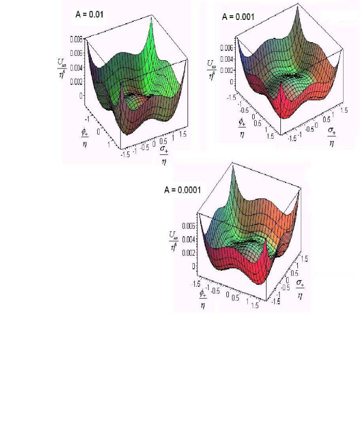
Figure 1: The potential of the superconducting cosmic string for some mixing paramenter $A$. The mixing parameters are in agreement with the cosmic string particle generation presented in [11].

4 The application to cosmic strings

Now, we analyse the crucial issue of gauge symmetry and supersymmetry breakings, and the consequent formation of a cosmic string configuration. The cosmic string that we have revised in Ref. [11], is determined in connection of the scalar potential $U_{CS}$ of the eq.(19). The minimum energy configuration of a static vortex potential for   $U_{scs}$   in   (19)  is   $<\phi_{+}>=\eta$ ,   $<\phi_{-}>=0$,       $<\sigma_{+}>=0$ and $<\sigma_{-}>=0$ ,   where   $\eta^{2}=\frac{2p}{q}v$   and   $v=\sqrt{[1+\frac{k^{2}}{p^{2}}+2\frac{Ak}{p}]}$, with the constraint given by

$$m^{2}=\frac{qp}{2\Gamma}(1+\frac{Ak}{p}-v)\,.$$ (23)

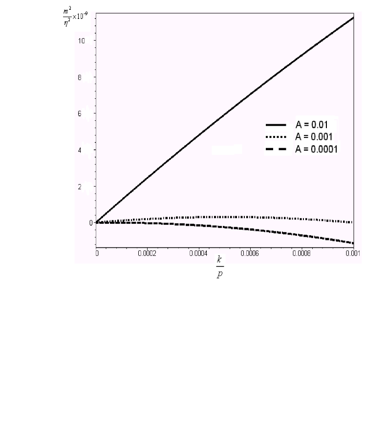
Figure 2: Plot of the ${m^{2}\over\eta^{2}}$ in function of the ${k\over p}$ to the $0\leq{k\over p}\leq 10^{-3}$.

To analyse the possibility that the parameters $m$ and $\eta$ give us a positive value, let us investigate the plot of ${m^{2}\over\eta^{2}}$ as a function of ${k\over p}$, given in Fig (2). We see that there is a region where it is possible to obtain a range of values for which $m^{2}$ and $\eta^{2}$ are both positive.

Then, it is possible to find the stable potential to the cosmic string without flat directions. The vacuum analysis of the potential gives us that it vanishes in its minimum. So, SUSY is not spontaneously broken in the vacuum. The U(1) symmetry related with the vortex field $\phi_{+}$ is broken, but the extra $U(1)^{\prime}$ symmetry related with the field $\sigma_{+}$ and $\sigma_{-}$ does not break and gives us an eletromagnetic propagation. In the core of the string, this scenario changes: $<\phi_{+}>=<\phi_{-}>=0$ and $<\sigma_{+}>=\sqrt{{2\over e}(Ap+k)}$. Then, the $U(1)^{\prime}$ breaking in the core gives us the bosonic particle condensate in the core. The potential does not vanish in these extrema, then the SUSY is broken in the core.

Until now, we have discussed only the spontaneous SUSY breaking. Now, let us explain in more details how the SUSY breaking appears in connection with the Lorentz breaking. To discuss this matter, let us recall that conventional Lorentz transformations are implemented as coordinate changes, and we usually refer to them as observer Lorentz transformations. However, we can also consider the so-called particle Lorentz transformations, which consist in applying boosts or rotations on particles and localised fields, but never on the background fields, contrary to the observer Lorentz transformations, which act also on ackground fields.

Distinguishing between observer and particle Lorentz transformations is crucial for the kind of model we are considering here, where the Chern-Simons term described in the Lagrangian of eq.(4) is to be regarded as arising from a constant background field, $S^{\mu}=i\partial^{\mu}(S-S^{*})$, which is to be seen as a global feature of the model, and is not related to localised experimental conditions, contrary the electromagnetic field, $A^{\mu}$, which is a perturbation that propagates in a space-time dominated by $S^{\mu}$. We note that this part only exists if $S$ has an imaginary part.

So, in applying particle Lorentz transformations, the gauge invariant Chern-Simons term of eq.(4) does not display Lorentz invariance, since $S^{\mu}$ is not acted upon by any $\Lambda$-matrix belonging to Lorentz group, so that the $\Lambda$’s acting on $\tilde{F}^{\mu\nu}$ and $A^{\alpha}$ do not combine to produce the $det\Lambda=1$-factor that would appear if $S^{\mu}$ were boosted, as it happens for the class of observer Lorentz transformations. In this particle frame, SUSY is broken. This detail shall be analysed in a forthcoming work, where we analyse the case of an imaginary part of $S$ were $S$. In this letter, we consider only the real part of $S$. If this is the case (Re $S\neq 0$, Im $S=0$), then the only effect of the background is to renomalise the gauge field kinetic term and the Lorentz-violation Maxwell-Chern-Simons does not show up; in such a situation, no violation of Lorentz symmetry is detected.

5 General conclusions

In this work, we study a general supersymmetric action to present a potential without flat directions. In our model, we study two aspects: a gauge-field mixing and the case with a Maxwell Chern-Simons term. We can compare these two possibilities and we see that in the Maxwell-Chern-Simons case, the potential has a minimum when the extra scalar field has a constant value. But, we pay attention to the fact that we only analyse the real part of this field, since its complex part does not contribute to the analysis of the breaking. Nevertheless, if we consider the complex part, we have other consequences to the model,such as the possibility of Lorentz symmetry breaking. If we analyse the Lagrangian (6) in components, we see that there appears a gauge-field mixing. A motivation to the study of these potentials is a cosmic string scenario. This approach is an alternative to the cosmic stirng potential without flat directions. In forthcoming works, we must analyse the potentials in connection with cosmic string, bosonic supercondutivity and Lorentz breaking effects for supersymmetric cosmic strings.

References

- [1] M. Cvetic and P. Langacker, Implications of abelian extended gauge structures from string models, Phys.Rev. D 54 (1996) 3570 [hep-ph/9511378]; New gauge bosons from string models, Mod.Phys.Lett. A 11 (1996) 12471247 [hep-ph/9602424].
- [2] M. Cvetic and P. Langacker, Perspectives on supersymmetry , G. L. Kane, Singapore 1998.
- [3] C. T. Hill and E. H. Simmons, Strong Dynamics and Electroweak Symmetry Breaking, Phys.Rept. 381 (2003) 235; Erratum-ibid. 390 (2004) 553 [hep-ph/0203079].
- [4] D. Suematsu and Y. Yamagishi, Radiative symmetry breaking in a supersymmeric model with an extra U(1), Int. J. Mod. Phys. A 10 (1995) 4521 [hep-ph/9411239].
- [5] M. Cevetic, D. A. Demir, J. R. Espinosa, L. L. Everett and P. Langacker, Electroweak breaking and the mu problem in supergravity models with an additional U(1), Phys. Rev. D 56 (1997) 2861; Erratum -ibid. D 58 (1997) 119905 [hep-ph/9703317] .
- [6] J. Ellis, J. F. Gunion, H. E. Haber, L. Roskowski, and F. Zwirner, Higgs bosons in a nonminimal supersymmetric model, Phys. Rev. D 39 (1989) 844; U. Ellwanger, J. F. Gunion, and C. Hugonie, Maximal temperature in flux compactifications, hep-ph/0111179.
- [7] L. Durand and J. L. Lopez,Upper bounds on higgs and top quark masses in the flipped Su(5) x U(1) superstring model, Phys. Lett. B 217 (1989) 463; M Drees, Supersymmetric models with extended higgs sector, Int. J. Mod. Phys. A 4 (1989) 3635.
- [8] J. Wess and J.Bagger, Supersymmetry and Supergravity, Princeton Series in Physics, Princeton 1992.
- [9] A. Vilenkin, Gravitational field of vacuum domain walls and strings, Phys. Rev. D 23 (1981) 852; W. A. Hiscock, Exact gravitational field of a string, Phys. Rev. D 31 (1985) 3288; J. R. Gott III, Gravitational lensing effects of vacuum strings: exact solutions, Ap. J. 288 (1985) 422; D. Garfinkel, General relativistic strings, Phys. Rev. D 32 (1985) 1323.
- [10] E. Witten, Superconducting strings, Nucl. Phys. B 249 (1985) 557; C. N. Ferreira, M. E. X. Guimarães and J. A. Helayël-Neto, Current-Carrying Cosmic Strings in Scalar-Tensor Gravities, Nucl.Phys. B 581 (2000) 165 [gr-qc/0002054]; V. B. Bezerra and C. N. Ferreira, Gravitational field around a screwed superconducting cosmic string in scalar-tensor theories, Phys.Rev. D 65 (2002) 084030 [hep-th/0111167]; C.N. Ferreira, Screwed superconducting cosmic strings, Class.Quant.Grav. 19 (2002) 741 [hep-th/0202105]; V. B. Bezerra, C. N. Ferreira, J. B. Fonseca-Neto and A. A. R. Sobreira, Gravitational field around a time-like current-carrying screwed cosmic string in scalar-tensor theories, Phys.Rev. D 68 (2003) 124020 [hep-th/0306289].
- [11] C.N. Ferreira, C.F.L. Godinho and J.A. Helayël-Neto, A Discussion on Supersymmetric Cosmic Strings with Gauge-Field Mixing, New J.Phys. 6 (2004) 58 [hep-th/0205035]; C. N. Ferreira, H. Chávez and J. A. Helayël-Neto, Cosmological Implications of Supersymmetric Superconducting Cosmic Strings Serie Horizons in World Physics, Novagating the World for Knowledge, to appear in (2005).
- [12] J. R. Morris, Supersymmetry and gauge invariance constraints in a U(1) x U(1)-prime higgs superconducting cosmic string model, Phys. Rev. D 53 (1996) 2078 [hep-ph/9511293].
- [13] S. C. Davis, A. C. Davis and M. Trodden, N=1 supersymmetric cosmic strings, Phys. Lett. B 405 (1997) 257 [hep-ph/9702360].
- [14] J. D. Edelstein, W. G. Fuertes, J. Mas. and J. M. Guilarte, Phases of dual superconductivity and confinement in softly broken n=2 supersymmetric yang-mills theories, Phys. Rev. D 62 (2000) 065008 [hep-th/0001184].
- [15] C. N. Fereira, J. A. Helayël-Neto and M. B. D. S. M. Porto, Cosmic string in the supersymmetric CSKR theory, Nucl. Phys. B 620 (2002) 181 [hep-th/0101008]; Topologically charged vortex in a supersymmetric Kalb-Ramond theory, Serie Horizons in World Physics, Novagating the World for Knowledge 244 (2004); N. R. F. Braga and C. N. Ferreira, Topological mass term in effective Brane-World scenario with torsion, hep-th/0410186.
- [16] G. Dvali and S. Kachru, New old inflation, hep-th/0309095; and whithout flat directions, A. Linde, Fast roll inflation, JHEP 0111 (2001) 052.
- [17] B. Zumino, Spontaneous Breaking of Supersymmetry, Lecture Notes in Physics 160 (1981).
- [18] R. Jackiw and P. Rossi, Zero modes of the vortex - fermion system, Nucl. Phys. B 190 (1981) 681; V. B. Bezerra, H. J. Mosquera Cuesta, C. N. Ferreira, Cosmic optical activity in the spacetime of a scalar-tensor screwed cosmic string, Phys.Rev. D 67 (2003) 084011 [hep-th/0210052]; H. Belich, J. L. Boldo, L. P. Colatto, J. A. Helayël-Neto and A. L. M. A. Nogueira, Supersymmetric extension of the lorentz and CPT violating Maxwell-Chern-Simons model, Phys. Rev. D 68 (2003) 065030 [hep-th/0304166].
- [19] I. I. Kogan, Induced magnetic moment for anyons Phys. Lett. B 262 (1991) 83; J. Stern, Topological action at a distance and the magnetic moment of point - like anyons, Phys.Lett. B 265 (1991) 119.
- [20] B. H. Lee, C. Lee, and H. Min, Supersymmetric chern-simons vortex systems and fermion zero modes, Phys. Rev. D 45 (1992) 4588.
- [21] Z. Hlousek and D. Spector, Why topological charges imply extended supersymmetry, Nucl. Phys. B 370 143, (1992); Bogomolny explained, Nucl. Phys. B 397 (1993) 173.
- [22] C. E. Carlson, C. D. Carone, R. F. Lebed, Supersymmetric noncommutative QED and lorentz violation, Phys.Lett. B 549 (2002) 337 [hep-ph/0209077]; K. Y. Kim, B.H. Lee and H. S. Yang, Zero modes and the Atiyah-singer index in noncommutative instantons, Phys.Rev., D 66 (2002) 025034 [hep-th/0205010]; A. Connes, M.R. Douglas and A.S. Achwarz, JHEP 02(1998) 003; R. Amorim, C. N. Ferreira, C. F. L. Godinho, The noncommutative U(N) Kalb-Ramond theory, Phys.Lett. B 593 (2004) 203 [hep-th/0403088]; R. Amorim, N. R. F. Braga, C. N. Ferreira, Nonequivalent Seiberg-Witten maps for noncommutative massive U(N) gauge theory, Phys.Lett. B 591 (2004) 181 [hep-th/0312089].
- [23] O. Piguet and K. Sibold Renormalized supersymmetry, Progress in Physics 12 (1986) .
- [24] A. A. Penin, V. A. Rubakov, P. G. Tiyakov and S. V. Troitsky, What becomes of vortices in theories with flat directions, Phys. Lett. B 389 (1996) 13 [hep-ph/9609257].