Abstract

The level crossing problem and associated geometric terms are neatly formulated by the second quantized formulation. This formulation exhibits a hidden local gauge symmetry related to the arbitrariness of the phase choice of the complete orthonormal basis set. By using this second quantized formulation, which does not assume adiabatic approximation, a convenient exact formula for the geometric terms including off-diagonal geometric terms is derived. The analysis of geometric phases is then reduced to a simple diagonalization of the Hamiltonian, and it is analyzed both in the operator and path integral formulations. If one diagonalizes the geometric terms in the infinitesimal neighborhood of level crossing, the geometric phases become trivial (and thus no monopole singularity) for arbitrarily large but finite time interval $T$. The integrability of Schrödinger equation and the appearance of the seemingly non-integrable phases are thus consistent. The topological proof of the Longuet-Higgins’ phase-change rule, for example, fails in the practical Born-Oppenheimer approximation where a large but finite ratio of two time scales is involved and $T$ is identified with the period of the slower system. The difference and similarity between the geometric phases associated with level crossing and the exact topological object such as the Aharonov-Bohm phase become clear in the present formulation. A crucial difference between the quantum anomaly and the geometric phases is also noted.

1 Introduction

The geometric phases are usually analyzed in the framework of first quantization by using the adiabatic approximation [1]-[13], though a non-adiabatic treatment has been considered in, for example, [8] and the (non-adiabatic) correction to the geometric phases has been analyzed in [9]. The Hamiltonian, which contains a set of slowly varying external parameters, has no obvious singularity by itself. But a singularity reminiscent of the magnetic monopole is induced at the level crossing point, which is controlled by the movement of the external parameters, and the associated geometric phases appear in the adiabatic approximation. A remarkable fact is that the geometric phase factors thus introduced are rather universal independently of detailed physical processes. The topological properties are considered to be responsible for this universal behavior. Also, interesting mathematical ideas such as parallel transport and holonomy are often used [2] in the framework of adiabatic approximation.

The geometric phases revealed the importance of hitherto un-recognized phase factors in the adiabatic approximation. It may then be interesting to investigate how those phases appear in the exact formulation. The purpose of the present paper is to formulate the level crossing problem by using the second quantization technique, which works both in the path integral and operator formulations. We thus derive a convenient exact formula for geometric terms, including the off-diagonal terms as well as the conventional diagonal terms. In this formulation, the analysis of geometric phases is reduced to the familiar diagonalization of the Hamiltonian. Namely, all the information concerning the extra phase factors is contained in the effective Hamiltonian. In Ref. [9], this fact that the geometric phases are interpreted as parts of the Hamiltonian has been noted though only the diagonal geometric terms have been analyzed in the adiabatic picture. Our formulation is more general without assuming the adiabatic picture.

When one diagonalizes the Hamiltonian in a very specific limit, one recovers the conventional geometric phases defined in the adiabatic approximation. One can thus analyze the geometric phases in the present formulation without using the mathematical notions such as parallel transport and holonomy. Instead, a hidden local gauge symmetry plays an important role in our formulation. If one diagonalizes the Hamiltonian in the other extreme limit, namely, in the infinitesimal neighborhood of level crossing for any fixed finite time interval $T$, one can show that the geometric phases become trivial and thus no monopole-like singularity. At the level crossing point, the conventional energy eigenvalues become degenerate but the degeneracy is lifted if one diagonalizes the geometric terms. Since the time interval involved in the practical physical processes is always finite, our analysis implies an important change in our understanding of the qualitative aspects of geometric phases. For example, our analysis implies that the topological interpretation [3, 1] of geometric phases such as the topological proof of the Longuet-Higgins’ phase-change rule [4] fails in the practical Born-Oppenheimer approximation where a large but finite ratio of two time scales is involved and $T$ is identified with the period of the slower system.

In our analysis, it is important to distinguish the precise adiabatic approximation, where the time interval $T$ measured in units of the shorter time scale is taken to be $T\rightarrow\infty$ [2], from the practical Born-Oppenheimer approximation where a large but finite ratio of two time scales is involved and the variables with the slower time scale are approximately treated as external c-number parameters. Our analysis shows that the integrability of the Schrödinger equation for a regular Hamiltonian and the appearance of the seemingly “non-integrable phases” are consistent: To be precise, the integrability of the Schrödinger equation becomes relevant when the slowly varying external parameters are promoted to the dynamical variables of a more fundamental regular Hamiltonian.

We also clarify the difference between the geometric phases associated with level crossing and the exact topological object such as the Aharonov-Bohm phase. A crucial difference between the quantum anomaly and the geometric phases associated with level crossing is also noted.

The basic idea involved in the present formulation has been reported elsewhere [14], and we here present further details of the analyses.

2 Second quantized formulation and geometric phases

We start with the generic (hermitian) Hamiltonian

$$\hat{H}=\hat{H}(\hat{\vec{p}},\hat{\vec{x}},X(t))$$ (2.1)

for a single particle theory in a slowly varying background variable $X(t)=(X_{1}(t),X_{2}(t),...)$. The path integral for this theory for the time interval $0\leq t\leq T$ in the second quantized formulation is given by

$$Z = \int{\cal D}\psi^{\star}{\cal D}\psi\exp\{\frac{i}{\hbar}\int_{0}^{T}dtd^{3}x[\psi^{\star}(t,\vec{x})i\hbar\frac{\partial}{\partial t}\psi(t,\vec{x})$$ (2.2)

$$-\psi^{\star}(t,\vec{x})\hat{H}(\frac{\hbar}{i}\frac{\partial}{\partial\vec{x}},\vec{x},X(t))\psi(t,\vec{x})]\}.$$

We then define a complete set of eigenfunctions

$$\hat{H}(\frac{\hbar}{i}\frac{\partial}{\partial\vec{x}},\vec{x},X(0))u_{n}(\vec{x},X(0))=\lambda_{n}u_{n}(\vec{x},X(0)),$$

$$\int d^{3}xu_{n}^{\star}(\vec{x},X(0))u_{m}(\vec{x},X(0))=\delta_{nm},$$ (2.3)

and expand

$$\psi(t,\vec{x})=\sum_{n}a_{n}(t)u_{n}(\vec{x},X(0)).$$ (2.4)

We then have

$${\cal D}\psi^{\star}{\cal D}\psi=\prod_{n}{\cal D}a_{n}^{\star}{\cal D}a_{n}$$ (2.5)

and the path integral is written as

$$Z = \int\prod_{n}{\cal D}a_{n}^{\star}{\cal D}a_{n}\exp\{\frac{i}{\hbar}\int_{0}^{T}dt[\sum_{n}a_{n}^{\star}(t)i\hbar\frac{\partial}{\partial t}a_{n}(t)$$ (2.6)

$$-\sum_{n,m}a_{n}^{\star}(t)E_{nm}(X(t))a_{m}(t)]\}$$

where

$$E_{nm}(X(t))=\int d^{3}xu_{n}^{\star}(\vec{x},X(0))\hat{H}(\frac{\hbar}{i}\frac{\partial}{\partial\vec{x}},\vec{x},X(t))u_{m}(\vec{x},X(0)).$$ (2.7)

We next perform a unitary transformation

$$a_{n}=\sum_{m}U(X(t))_{nm}b_{m}$$ (2.8)

where

$$U(X(t))_{nm}=\int d^{3}xu^{\star}_{n}(\vec{x},X(0))v_{m}(\vec{x},X(t))$$ (2.9)

with the instantaneous eigenfunctions of the Hamiltonian

$$\hat{H}(\frac{\hbar}{i}\frac{\partial}{\partial\vec{x}},\vec{x},X(t))v_{n}(\vec{x},X(t))={\cal E}_{n}(X(t))v_{n}(\vec{x},X(t)),$$

$$\int d^{3}xv^{\star}_{n}(\vec{x},X(t))v_{m}(\vec{x},X(t))=\delta_{n,m}.$$ (2.10)

We emphasize that $U(X(t))$ is a unit matrix both at $t=0$ and $t=T$ if $X(T)=X(0)$, and thus

$$\{a_{n}\}=\{b_{n}\}$$ (2.11)

both at $t=0$ and $t=T$. We take the time $T$ as a period of the slowly varying variable $X(t)$. We can thus re-write the path integral as

$$Z=\int\prod_{n}{\cal D}b_{n}^{\star}{\cal D}b_{n}\exp\{\frac{i}{\hbar}\int_{0}^{T}dt[\sum_{n}b_{n}^{\star}(t)i\hbar\frac{\partial}{\partial t}b_{n}(t)$$

$$+\sum_{n,m}b_{n}^{\star}(t)\langle n|i\hbar\frac{\partial}{\partial t}|m\rangle b_{m}(t)-\sum_{n}b_{n}^{\star}(t){\cal E}_{n}(X(t))b_{n}(t)]\}$$ (2.12)

where the second term in the action stands for the term commonly referred to as Berry’s phase[1] and its off-diagonal generalization. The second term in (2.12) is defined by

$$(U(X(t))^{\dagger}i\hbar\frac{\partial}{\partial t}U(X(t)))_{nm} = \int d^{3}xv^{\star}_{n}(\vec{x},X(t))i\hbar\frac{\partial}{\partial t}v_{m}(\vec{x},X(t))$$ (2.13)

$$\equiv \langle n|i\hbar\frac{\partial}{\partial t}|m\rangle.$$

The path integral (2.12) is also derived directly by expanding $\psi(t,\vec{x})=\sum_{n}b_{n}(t)v_{n}(\vec{x},X(t))$ in terms of the instantaneous eigenfunctions in (2.10). As for the phase choice of $v_{n}(\vec{x},X(t))$ in (2.10), it will be discussed in detail later in connection with the hidden local gauge symmetry. As we already mentioned, the fact that the Berry’s phase can be understood as a part of the Hamiltonian, i.e.,dynamical, has been noted in an adiabatic picture [9]. Our formula does not assume the adiabatic approximation, and thus it gives a generalization.

In the operator formulation of the second quantized theory, we thus obtain the effective Hamiltonian (depending on Bose or Fermi statistics)

$$\hat{H}_{eff}(t) = \sum_{n}\hat{b}_{n}^{\dagger}(t){\cal E}_{n}(X(t))\hat{b}_{n}(t)$$ (2.14)

$$-\sum_{n,m}\hat{b}_{n}^{\dagger}(t)\langle n|i\hbar\frac{\partial}{\partial t}|m\rangle\hat{b}_{m}(t)$$

with

$$[\hat{b}_{n}(t),\hat{b}^{\dagger}_{m}(t)]_{\mp}=\delta_{n,m}.$$ (2.15)

Note that these formulas (2.6), (2.12) and (2.14) are exact and, to our knowledge, the formulas (2.12) and (2.14) have not been analyzed before . See, however, eq.(2) in ref.[7]. The off-diagonal geometric terms in (2.14), which are crucial in the analysis below, are missing in the usual adiabatic approximation in the first quantization. The use of the instantaneous eigenfunctions in (2.12) is a common feature shared with the adiabatic approximation. In our picture, all the information about geometric phases is included in the effective Hamiltonian, and for this reason we use the terminology “geometric terms” for those general terms appearing in the Hamiltonian. The “geometric phases” are used when these terms are interpreted as phase factors of a specific state vector.

Since our formulation starts with the path integral representation (2.2), the equivalence of the present exact formulation to the more conventional representation is expected. It may however be nice to check this equivalence explicitly. We define the “Schrödinger” picture by noting the Heisenberg equation of motion

$$i\hbar\frac{\partial}{\partial t}\hat{b}_{n}(t)=[\hat{b}_{n}(t),\hat{H}_{eff}(t)]$$ (2.16)

and thus introducing a unitary operator $U(t)$ by

$$i\hbar\frac{\partial}{\partial t}U(t)=-\hat{H}_{eff}(t)U(t)$$ (2.17)

with $U(0)=1$. We then have

$$\hat{b}_{n}(t) = U(t)\hat{b}_{n}(0)U(t)^{\dagger},$$

$$\hat{{\cal H}}_{eff}(t) \equiv U(t)^{\dagger}\hat{H}_{eff}(t)U(t)$$ (2.18)

$$= \sum_{n}\hat{b}_{n}^{\dagger}(0){\cal E}_{n}(X(t))\hat{b}_{n}(0)-\sum_{n,m}\hat{b}_{n}^{\dagger}(0)\langle n|i\hbar\frac{\partial}{\partial t}|m\rangle\hat{b}_{m}(0).$$

We note that the state vectors in the Heisenberg and Schrödinger pictures are related by

$$\Psi_{H}(0)=U(t)\Psi_{S}(t)$$ (2.19)

and thus

$$i\hbar\frac{\partial}{\partial t}\Psi_{S}(t)=U^{\dagger}(t)\hat{H}_{eff}(t)U(t)U^{\dagger}(t)\Psi_{H}(0)=\hat{{\cal H}}_{eff}(t)\Psi_{S}(t).$$ (2.20)

The second quantization formula for the evolution operator then gives rise to

$$\langle n|T^{\star}\exp\{-\frac{i}{\hbar}\int_{0}^{T}\hat{{\cal H}}_{eff}(t)dt\}|n\rangle$$

$$= \langle n|T^{\star}\exp\{-\frac{i}{\hbar}\int_{0}^{T}dt[\sum_{n}\hat{b}_{n}^{\dagger}(0){\cal E}_{n}(X(t))\hat{b}_{n}(0)-\sum_{n,m}\hat{b}_{n}^{\dagger}(0)\langle n|i\hbar\frac{\partial}{\partial t}|m\rangle\hat{b}_{m}(0)]\}|n\rangle$$

$$= \sum_{n_{1},n_{2},....,n_{N}}$$

$$\langle n|\exp\{-\frac{i\epsilon}{\hbar}[\sum_{n}\hat{b}_{n}^{\dagger}(0){\cal E}_{n}(X(T))\hat{b}_{n}(0)-\sum_{n,m}\hat{b}_{n}^{\dagger}(0)\langle n|i\hbar\frac{\partial}{\partial T}|m\rangle\hat{b}_{m}(0)]\}|n_{1}\rangle$$

$$\times \langle n_{1}|\exp\{-\frac{i\epsilon}{\hbar}[\sum_{n}\hat{b}_{n}^{\dagger}(0){\cal E}_{n}(X(t_{1}))\hat{b}_{n}(0)-\sum_{n,m}\hat{b}_{n}^{\dagger}(0)\langle n|i\hbar\frac{\partial}{\partial t_{1}}|m\rangle\hat{b}_{m}(0)]\}|n_{2}\rangle$$

$$\times \langle n_{2}|\exp\{-\frac{i\epsilon}{\hbar}[\sum_{n}\hat{b}_{n}^{\dagger}(0){\cal E}_{n}(X(t_{2}))\hat{b}_{n}(0)-\sum_{n,m}\hat{b}_{n}^{\dagger}(0)\langle n|i\hbar\frac{\partial}{\partial t_{2}}|m\rangle\hat{b}_{m}(0)]\}|n_{3}\rangle$$

$$\times .....$$

$$\times \langle n_{N}|\exp\{-\frac{i\epsilon}{\hbar}[\sum_{n}\hat{b}_{n}^{\dagger}(0){\cal E}_{n}(X(t_{N}))\hat{b}_{n}(0)-\sum_{n,m}\hat{b}_{n}^{\dagger}(0)\langle n|i\hbar\frac{\partial}{\partial t_{N}}|m\rangle\hat{b}_{m}(0)]\}|n\rangle$$

where $T^{\star}$ stands for the time ordering operation and $\epsilon=T/(N+1)$, and the state vectors in the second quantization are defined by

$$|n\rangle=\hat{b}_{n}^{\dagger}(0)|0\rangle.$$ (2.22)

This formula is re-written as

$$\sum_{n_{1},n_{2},....,n_{N}}[\exp\{-\frac{i\epsilon}{\hbar}[{\cal E}_{n}(X(T))-\langle n|i\hbar\frac{\partial}{\partial T}|n_{1}\rangle]\}\delta_{n,n_{1}}+\frac{i\epsilon}{\hbar}\langle n|i\hbar\frac{\partial}{\partial T}|n_{1}\rangle|_{n\neq n_{1}}]$$ (2.23)

$$\times [\exp\{-\frac{i\epsilon}{\hbar}[{\cal E}_{n_{1}}(X(t_{1}))-\langle n_{1}|i\hbar\frac{\partial}{\partial t_{1}}|n_{2}\rangle]\}\delta_{n_{1},n_{2}}+\frac{i\epsilon}{\hbar}\langle n_{1}|i\hbar\frac{\partial}{\partial t_{1}}|n_{2}\rangle|_{n_{1}\neq n_{2}}]$$

$$\times [\exp\{-\frac{i\epsilon}{\hbar}[{\cal E}_{n_{2}}(X(t_{2}))-\langle n_{2}|i\hbar\frac{\partial}{\partial t_{2}}|n_{3}\rangle]\}\delta_{n_{2},n_{3}}+\frac{i\epsilon}{\hbar}\langle n_{2}|i\hbar\frac{\partial}{\partial t_{2}}|n_{3}\rangle|_{n_{2}\neq n_{3}}]$$

$$\times .....$$

$$\times [\exp\{-\frac{i\epsilon}{\hbar}[{\cal E}_{n}(X(t_{N}))-\langle n_{N}|i\hbar\frac{\partial}{\partial t_{N}}|n\rangle]\}\delta_{n_{N},n}+\frac{i\epsilon}{\hbar}\langle n_{N}|i\hbar\frac{\partial}{\partial t_{N}}|n\rangle|_{n_{N}\neq n}]$$

where the state vectors in this last expression stand for the first quantized states defined by

$$\hat{H}(\hat{\vec{p}},\hat{\vec{x}},X(t))|n(t)\rangle={\cal E}_{n}(X(t))|n(t)\rangle,$$ (2.24)

and those state vectors also appear in the definition of geometric terms. If one retains only the diagonal elements in this formula (2.23), one recovers the conventional adiabatic formula [6]

$$\exp\{-\frac{i}{\hbar}\int_{0}^{T}dt[{\cal E}_{n}(X(t))-\langle n|i\hbar\frac{\partial}{\partial t}|n\rangle]\}.$$ (2.25)

On the other hand, if one retains the off-diagonal elements also, one obtains the exact evolution operator. We first observe, for example,

$$\exp\{-\frac{i\epsilon}{\hbar}[{\cal E}_{n_{1}}(X(t_{1}))-\langle n_{1}|i\hbar\frac{\partial}{\partial t_{1}}|n_{2}\rangle]\}\delta_{n_{1},n_{2}}+\frac{i\epsilon}{\hbar}\langle n_{1}|i\hbar\frac{\partial}{\partial t_{1}}|n_{2}\rangle|_{n_{1}\neq n_{2}}$$ (2.26)

$$= \exp\{-\frac{i\epsilon}{\hbar}{\cal E}_{n_{1}}(X(t_{1}))\}\langle n_{1}(t_{1})|n_{2}(t_{1}-\epsilon)\rangle+O(\epsilon^{2})$$

$$= \langle n_{1}(t_{1})|\exp\{-\frac{i\epsilon}{\hbar}\hat{H}(\hat{\vec{p}},\hat{\vec{x}},X(t_{1}))\}|n_{2}(t_{1}-\epsilon)\rangle+O(\epsilon^{2}).$$

By letting $\epsilon\rightarrow 0$, we thus obtain

$$\langle n|T^{\star}\exp\{-\frac{i}{\hbar}\int_{0}^{T}\hat{{\cal H}}_{eff}(t)dt\}|n\rangle$$

$$=\langle n(T)|T^{\star}\exp\{-\frac{i}{\hbar}\int_{0}^{T}\hat{H}(\hat{\vec{p}},\hat{\vec{x}},X(t))dt\}|n(0)\rangle\,.$$ (2.27)

Both-hand sides of this formula are exact, but the difference is that the geometric terms, both of diagonal and off-diagonal, are explicit in the second quantized formulation on the left-hand side.

Here we would like to comment on the possible advantages of using the second quantization technique. As we have already mentioned, all the results of the second quantization are in principle reproduced by the first quantization in the present single-particle problem. This fact is exemplified by the relation (2.27). The possible advantages are thus mainly technical and conceptual ones. First of all, the general geometric terms are explicitly and neatly formulated by the second quantization both for the path integral (2.12) and the operator formalism (2.27). Also, our emphasis is on the diagonalization of the Hamiltonian rather than on the subtle notion of phases. This emphasis on the Hamiltonian is also manifest in the second quantization on the left-hand side of (2.27). Another technical advantage in the present formulation is related to the phase freedom of the basis set in (2.10). The path integral formula (2.12) is based on the expansion

$$\psi(t,\vec{x})=\sum_{n}b_{n}(t)v_{n}(\vec{x},X(t)),$$ (2.28)

and the starting path integral (2.2) depends only on the field variable $\psi(t,\vec{x})$, not on $\{b_{n}(t)\}$ and $\{v_{n}(\vec{x},X(t))\}$ separately. This fact shows that our formulation contains a hidden local gauge symmetry

$$v_{n}(\vec{x},X(t))\rightarrow v^{\prime}_{n}(\vec{x},X(t))=e^{i\alpha_{n}(t)}v_{n}(\vec{x},X(t)),\ \ \ \ b_{n}(t)\rightarrow b^{\prime}_{n}(t)=e^{-i\alpha_{n}(t)}b_{n}(t)$$ (2.29)

where the gauge parameter $\alpha_{n}(t)$ is a general function of $t$. One can confirm that both of the path integral measure and the action in (2.12) are invariant under this gauge transformation. By using this gauge freedom, one can choose the phase convention of the basis set $\{v_{n}(\vec{x},X(t))\}$ such that the analysis of geometric phases becomes most transparent ; in (3.4) later, we choose the basis set $\{v_{n}(y(t))\}$ such that the artificial singularity introduced by the use of polar coordinates becomes minimum. The meaning of this gauge transformation shall be explained further in connection with equations (3.12) and (3.21).

The expression on the right-hand side of (2.27) stands for the first quantized formula which has an exact path integral representation given by

$$\langle n(T)|T^{\star}\exp\{-\frac{i}{\hbar}\int_{0}^{T}\hat{H}(\hat{\vec{p}},\hat{\vec{x}},X(t))dt\}|n(0)\rangle$$ (2.30)

$$= \iint d^{3}x(T)d^{3}x(0)u_{n}^{\star}(\vec{x}(T))u_{n}(\vec{x}(0))$$

$$\times\langle\vec{x}(T)|T^{\star}\exp\{-\frac{i}{\hbar}\int_{0}^{T}\hat{H}(\hat{\vec{p}},\hat{\vec{x}},X(t))dt\}|\vec{x}(0)\rangle$$

and

$$\langle\vec{x}(T)|T^{\star}\exp\{-\frac{i}{\hbar}\int_{0}^{T}\hat{H}(\hat{\vec{p}},\hat{\vec{x}},X(t))dt\}|\vec{x}(0)\rangle$$ (2.31)

$$= \int_{\vec{x}(0)}^{\vec{x}(T)}{\cal D}\vec{x}{\cal D}\vec{p}\exp\{\frac{i}{\hbar}\int_{0}^{T}dt[\vec{p}\cdot\dot{\vec{x}}-H(\vec{p},\vec{x},X(t))]\}$$

$$= \int_{\vec{x}(0)}^{\vec{x}(T)}{\cal D}\vec{x}{\cal D}\vec{p}\exp\{\frac{i}{\hbar}\int_{0}^{T}dt[\vec{p}\cdot\dot{\vec{x}}-H(\vec{p},\vec{x},0)-\sum_{l}H_{l}(\vec{p},\vec{x})X_{l}(t)]\}$$

where the last expression is valid for sufficiently small $X(t)=(X_{1}(t),X_{2}(t),...)$. In the analysis of level crossing, it is convenient to assume that the specific level crossing we are interested in takes place at the origin of $X(t)$ with

$$H_{l}(\vec{p},\vec{x})=\frac{\partial H(\vec{p},\vec{x},X(t))}{\partial X_{l}(t)}|_{X(t)=0}.$$ (2.32)

We note that the path integral (2.31) shows no obvious singular behavior at the level crossing point $X(t)=0$.

3 Level crossing and geometric phases

We are mainly interested in the topological properties of geometric phases. To simplify the analysis, we now assume that the level crossing takes place only between the lowest two levels, and we consider the familiar idealized model with only the lowest two levels. This simplification is expected to be valid to analyze the topological properties in the infinitesimal neighborhood of level crossing. The effective Hamiltonian to be analyzed in the path integral (2.6) is then defined by the $2\times 2$ matrix $h(X(t))=\left(E_{nm}(X(t))\right)$. If one assumes that the level crossing takes place at the origin of the parameter space $X(t)=0$, one needs to analyze the matrix

$$h(X(t))=\left(E_{nm}(0)\right)+\left(\frac{\partial}{\partial X_{k}}E_{nm}(X)|_{X=0}\right)X_{k}(t)$$ (3.1)

for sufficiently small $(X_{1}(1),X_{2}(1),...)$. By a time independent unitary transformation, which does not induce an extra geometric term, the first term is diagonalized. In the present approximation, essentially the four dimensional sub-space of the parameter space is relevant, and after a suitable re-definition of the parameters by taking linear combinations of $X_{k}(t)$, we write the matrix as [1]

$$h(X(t)) = \left(\begin{array}[]{cc}E(0)+y_{0}(t)&0\\ 0&E(0)+y_{0}(t)\end{array}\right)+g\sigma^{l}y_{l}(t)$$ (3.4)

where $\sigma^{l}$ stands for the Pauli matrices, and $g$ is a suitable (positive) coupling constant. This parametrization in terms of the variables $y_{l}$ is valid beyond the linear approximation, but the two-level approximation is expected to be valid only near the level crossing point.

The above matrix is diagonalized in the standard way as

$$h(X(t))v_{\pm}(y)=(E(0)+y_{0}(t)\pm gr)v_{\pm}(y)$$ (3.6)

where $r=\sqrt{y^{2}_{1}+y^{2}_{2}+y^{2}_{3}}$ and

$$v_{+}(y)=\left(\begin{array}[]{c}\cos\frac{\theta}{2}e^{-i\varphi}\\ \sin\frac{\theta}{2}\end{array}\right),\ \ \ \ \ v_{-}(y)=\left(\begin{array}[]{c}\sin\frac{\theta}{2}e^{-i\varphi}\\ -\cos\frac{\theta}{2}\end{array}\right)$$ (3.11)

by using the polar coordinates, $y_{1}=r\sin\theta\cos\varphi,\ y_{2}=r\sin\theta\sin\varphi,\ y_{3}=r\cos\theta$. Note that

$$v_{\pm}(y(0))=v_{\pm}(y(T))$$ (3.12)

if $y(0)=y(T)$ except for $(y_{1},y_{2},y_{3})=(0,0,0)$, and $\theta=0\ {\rm or}\ \pi$; when one analyzes the behavior near those singular points, due care needs to be exercised. If one defines

$$v^{\dagger}_{m}(y)i\frac{\partial}{\partial t}v_{n}(y)=A_{mn}^{k}(y)\dot{y}_{k}$$ (3.13)

where $m$ and $n$ run over $\pm$, we have

$$A_{++}^{k}(y)\dot{y}_{k} = \frac{(1+\cos\theta)}{2}\dot{\varphi}$$

$$A_{+-}^{k}(y)\dot{y}_{k} = \frac{\sin\theta}{2}\dot{\varphi}+\frac{i}{2}\dot{\theta}=(A_{-+}^{k}(y)\dot{y}_{k})^{\star},$$

$$A_{--}^{k}(y)\dot{y}_{k} = \frac{1-\cos\theta}{2}\dot{\varphi}.$$ (3.14)

The effective Hamiltonian (2.14) is then given by

$$\hat{H}_{eff}(t) = (E(0)+y_{0}(t)+gr(t))\hat{b}^{\dagger}_{+}\hat{b}_{+}$$ (3.15)

$$+ (E(0)+y_{0}(t)-gr(t))\hat{b}^{\dagger}_{-}\hat{b}_{-}-\hbar\sum_{m,n}\hat{b}^{\dagger}_{m}A^{k}_{mn}(y)\dot{y}_{k}\hat{b}_{n}.$$

In the conventional adiabatic approximation, one approximates the effective Hamiltonian (3.8) by

$$\hat{H}_{eff}(t) \simeq (E(0)+y_{0}(t)+gr(t))\hat{b}^{\dagger}_{+}\hat{b}_{+}$$ (3.16)

$$+(E(0)+y_{0}(t)-gr(t))\hat{b}^{\dagger}_{-}\hat{b}_{-}$$

$$-\hbar[\hat{b}^{\dagger}_{+}A^{k}_{++}(y)\dot{y}_{k}\hat{b}_{+}+\hat{b}^{\dagger}_{-}A^{k}_{--}(y)\dot{y}_{k}\hat{b}_{-}]$$

which is valid for

$$Tgr(t)\gg\hbar\pi,$$

where $\hbar\pi$ stands for the magnitude of the geometric term times $T$. The Hamiltonian for $b_{-}$, for example, is then eliminated by a “gauge transformation”

$$b_{-}(t)=\exp\{-(i/\hbar)\int_{0}^{t}dt[E(0)+y_{0}(t)-gr(t)-\hbar A^{k}_{--}(y)\dot{y}_{k}]\}\tilde{b}_{-}(t)$$ (3.17)

in the path integral (2.12) with the above approximation (3.9), and the amplitude $\langle 0|\hat{\psi}(T)\hat{b}^{\dagger}_{-}(0)|0\rangle$, which corresponds to the probability amplitude in the first quantization, is given by (up to an eigenfunction $\phi_{E}(\vec{x})$ of $\hat{H}(\frac{\hbar}{i}\frac{\partial}{\partial\vec{x}},\vec{x},0)$ in (2.3))

$$\psi_{-}(T) \equiv \langle 0|\hat{\psi}(T)\hat{b}^{\dagger}_{-}(0)|0\rangle$$ (3.18)

$$= \exp\{-\frac{i}{\hbar}\int_{0}^{T}dt[E(0)+y_{0}(t)-gr(t)-\hbar A^{k}_{--}(y)\dot{y}_{k}]\}v_{-}(y(T))$$

$$\times\langle 0|\hat{\tilde{b}}_{-}(T)\hat{\tilde{b}}{}^{\dagger}_{-}(0)|0\rangle$$

$$= \exp\{-\frac{i}{\hbar}\int_{0}^{T}dt[E(0)+y_{0}(t)-gr(t)-\hbar A^{k}_{--}(y)\dot{y}_{k}]\}v_{-}(y(T))$$

with $\langle 0|\hat{\tilde{b}}_{-}(T)\hat{\tilde{b}}{}^{\dagger}_{-}(0)|0\rangle=\langle 0|\hat{\tilde{b}}_{-}(0)\hat{\tilde{b}}{}^{\dagger}_{-}(0)|0\rangle=1$. For a $2\pi$ rotation in $\varphi$ with fixed $\theta$, for example, the geometric term gives rise to the well-known factor 

$$\psi_{-}(T)=\exp\{i\pi(1-\cos\theta)\}\exp\{-\frac{i}{\hbar}\int_{C(0\rightarrow T)}dt[E(0)+y_{0}(t)-gr(t)]\}v_{-}(y(T))$$ (3.19)

by using (3.7) [1], and the path $C(0\rightarrow T)$ specifies the integration along the above specific closed path. Note that $v_{-}(y(T))=v_{-}(y(0))$ in the present choice of the basis set, and thus (3.12) can also be written as

$$\psi_{-}(T)=\exp\{i\pi(1-\cos\theta)\}\exp\{-\frac{i}{\hbar}\int_{C(0\rightarrow T)}dt[E(0)+y_{0}(t)-gr(t)]\}\psi_{-}(0)$$

The correction to the formula (3.12) arising from the finite $1/T$ may be analyzed by an iterative procedure [9], for example. One can thus analyze the geometric phase in the present formulation without using the mathematical notions such as parallel transport and holonomy.

Another representation, which is useful to analyze the behavior near the level crossing point, is obtained by a further unitary transformation

$$\hat{b}_{m}=\sum_{n}U(\theta(t))_{mn}\hat{c}_{n}$$ (3.20)

where $m,n$ run over $\pm$ with

$$U(\theta(t))=\left(\begin{array}[]{cc}\cos\frac{\theta}{2}&-\sin\frac{\theta}{2}\\ \sin\frac{\theta}{2}&\cos\frac{\theta}{2}\end{array}\right),$$ (3.23)

and the above effective Hamiltonian (3.8) is written as

$$\hat{H}_{eff}(t) =(E(0)+y_{0}(t)+gr\cos\theta)\hat{c}^{\dagger}_{+}\hat{c}_{+}$$ (3.24)

$$+(E(0)+y_{0}(t)-gr\cos\theta)\hat{c}^{\dagger}_{-}\hat{c}_{-}$$

$$-gr\sin\theta\hat{c}^{\dagger}_{+}\hat{c}_{-}-gr\sin\theta\hat{c}^{\dagger}_{-}\hat{c}_{+}-\hbar\dot{\varphi}\hat{c}^{\dagger}_{+}\hat{c}_{+}.$$

In the above unitary transformation, an extra geometric term $-U(\theta)^{\dagger}i\hbar\partial_{t}U(\theta)$ is induced by the kinetic term of the path integral representation (2.12). One can confirm that this extra term precisely cancels the term containing $\dot{\theta}$ in $\hat{b}^{\dagger}_{m}A^{k}_{mn}(y)\dot{y}_{k}\hat{b}_{n}$ as in (3.7). We thus diagonalize the geometric terms in this representation. We also note that $U(\theta(T))=U(\theta(0))$ if $X(T)=X(0)$ except for the origin, and thus the initial and final states receive the same transformation in scattering amplitudes. The above diagonalization of the geometric terms corresponds to the use of eigenfunctions

$$w_{m}=\sum_{n}U(\theta(t))^{\dagger}_{mn}v_{n}$$ (3.25)

or explicitly

$$w_{+}=\left(\begin{array}[]{c}e^{-i\varphi}\\ 0\end{array}\right),\ \ \ \ \ w_{-}=\left(\begin{array}[]{c}0\\ 1\end{array}\right)$$ (3.30)

in the definition of geometric terms. In the infinitesimal neighborhood of the level crossing point, namely, for sufficiently close to the origin of the parameter space $(y_{1}(t),y_{2}(t),y_{3}(t))$ but $(y_{1}(t),y_{2}(t),y_{3}(t))\neq(0,0,0)$, one may approximate (3.15) by

$$\hat{H}_{eff}(t) \simeq (E(0)+y_{0}(t)+gr\cos\theta)\hat{c}^{\dagger}_{+}\hat{c}_{+}$$ (3.31)

$$+ (E(0)+y_{0}(t)-gr\cos\theta)\hat{c}^{\dagger}_{-}\hat{c}_{-}-\hbar\dot{\varphi}\hat{c}^{\dagger}_{+}\hat{c}_{+}.$$

To be precise, for any given fixed time interval $T$,

$$T\hbar\dot{\varphi}\sim 2\pi\hbar$$ (3.32)

which is invariant under the uniform scale transformation $y_{k}(t)\rightarrow\epsilon y_{k}(t)$. On the other hand, one has $Tgr\sin\theta\rightarrow T\epsilon gr\sin\theta$ by the above scaling, and thus one can choose

$$T\epsilon gr\ll\hbar.$$

The terms $\pm gr\cos\theta$ in (3.18) may also be ignored in the present approximation.

In this new basis (3.18), the geometric phase appears only for the mode $\hat{c}_{+}$ which gives rise to a phase factor

$$\exp\{i\int_{C}\dot{\varphi}dt\}=\exp\{2i\pi\}=1,$$ (3.33)

and thus no physical effects. In the infinitesimal neighborhood of level crossing, the states spanned by $(\hat{b}_{+},\hat{b}_{-})$ are transformed to a linear combination of the states spanned by $(\hat{c}_{+},\hat{c}_{-})$, which give no non-trivial geometric phases. The geometric terms are topological in the sense that they are invariant under the uniform scaling of $y_{k}(t)$, but their physical implications in conjunction with other terms in the effective Hamiltonian are not. For example, starting with the state $\hat{b}^{\dagger}_{-}(0)|0\rangle$ one may first make $r\rightarrow small$ with fixed $\theta$ and $\varphi$, then make a $2\pi$ rotation in $\varphi$ in the bases $\hat{c}^{\dagger}_{\pm}|0\rangle$, and then come back to the original $r$ with fixed $\theta$ and $\varphi$ for a given fixed $T$ as in Fig.1 ; in this cycle, one does not pick up any non-trivial geometric phase even though one covers the solid angle $2\pi(1-\cos\theta)$.

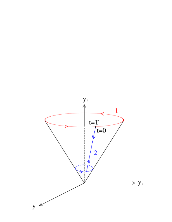
Fig. 1: (Color online) The path 1 gives the conventional geometric phase as in (3.12) for a fixed finite $T$, whereas the path 2 gives a trivial phase for a fixed finite $T$. Note that both of the paths cover the same solid angle $2\pi(1-\cos\theta)$.

To be precise, the physical quantity in (3.12) is replaced by

$$\psi_{-}(T) = \exp\{-\frac{i}{\hbar}\int_{C_{2}(0\rightarrow T)}dt[E(0)+y_{0}(t)-gr(t)-\hbar A^{k}_{--}(y)\dot{y}_{k}]\}v_{-}(y(T))$$ (3.34)

$$= \exp\{-\frac{i}{\hbar}\int_{C_{2}(0\rightarrow T)}dt[E(0)+y_{0}(t)-gr(t)]\}v_{-}(y(T))$$

by deforming the path 1 to the path 2 in the parameter space in Fig. 1. The path $C_{2}(0\rightarrow T)$ specifies the path 2 in Fig.1, and $v_{-}(y(T))=v_{-}(y(0))=\psi_{-}(0)$ in the present specific choice of the basis set. The first expression in the above equation explicitly shows the invariance of $\psi_{-}(T)$ under the gauge transformation (2.29) up to a trivial overall constant phase . The transformation from $\hat{b}_{\pm}$ to $\hat{c}_{\pm}$ is highly non-perturbative, since a complete re-arrangement of two levels is involved.

It should be noted that one cannot simultaneously diagonalize the conventional energy eigenvalues and the induced geometric terms in (3.8) which is exact in the present two-level model (3.2). The topological considerations [3, 1] are thus inevitably approximate. In this respect, it may be instructive to consider a model without level crossing which is defined by setting

$$y_{3}=\Delta E/2g$$ (3.38)

in (3.8), where $\Delta E$ stands for the minimum of the level spacing. The geometric terms then loose invariance under the uniform scaling of $y_{1}$ and $y_{2}$. In the limit

$$\sqrt{y^{2}_{1}+y^{2}_{2}}\gg\Delta E/2g,$$ (3.39)

$\theta\rightarrow\pi/2$ and the geometric terms in (3.8) exhibit approximately topological behavior for the reduced variables $(y_{1},y_{2})$: One can thus perform an approximate topological analysis of the phase change rule. Near the point where the level spacing becomes minimum, which is specified by

$$(y_{1},y_{2})\rightarrow(0,0)$$ (3.40)

(and thus $\theta\rightarrow 0$), the geometric terms in (3.8) assume the form of the geometric term in (3.18) and thus the geometric phases become trivial. Our analysis shows that the model with level crossing (3.2) exhibits precisely the same topological properties for any finite $T$.

It is instructive to analyze an explicit example in Refs. [15, 16] where the following parametrization has been introduced

$$(y_{1},y_{2},y_{3})=(B_{0}(b_{1}+\cos\omega t),B_{0}\sin\omega t,B_{z})$$ (3.41)

and $g=\mu$ in the notation of (3.2). The case $b_{1}=0$ and $B_{z}\neq 0$ corresponds to the model without level crossing discussed above in (3.22), and the geometric phase becomes trivial for $B_{0}\rightarrow 0$.

Fig. 2: (Color online) The path 1 for $(y_{1},y_{2},y_{3})=(B_{0}\cos\omega t,B_{0}\sin\omega t,0)$ gives rise to the phase change rule for a fixed finite $T=2\pi/\omega$ and $\mu B_{0}/\hbar\omega\gg 1$, whereas the path 2 gives a trivial phase for a fixed finite $T$ and $\mu B_{0}/\hbar\omega\ll 1$, thus resulting in the failure of the topological argument for the phase change rule for any fixed finite $T$.

The case $b_{1}=B_{z}=0$ describes the model with level crossing: The case $b_{1}=B_{z}=0$ with

$$T=2\pi/\omega$$ (3.42)

kept fixed describes the situation in (3.18) with $\theta=\pi/2$, namely, a closed cycle in the infinitesimal neighborhood of level crossing for $B_{0}\rightarrow 0$, and the geometric phase becomes trivial. See Fig.2. To be explicit,

$$\psi_{-}(T) = \exp\{-\frac{i}{\hbar}\int_{C_{1}}dt[E(0)+y_{0}(t)-\mu B_{0}-\hbar A^{k}_{--}(y)\dot{y}_{k}]\}v_{-}(y(T))$$ (3.45)

$$= (-1)\exp\{-\frac{i}{\hbar}\int_{C_{1}}dt[E(0)+y_{0}(t)-\mu B_{0}]\}\frac{1}{\sqrt{2}}\left(\begin{array}[]{c}e^{-i\varphi(T)}\\ -1\end{array}\right)$$

for the path 1 with $\mu B_{0}/\hbar\omega\gg 1$ where the factor $(-1)$ stands for the Longuet-Higgins’ phase change [4], and

$$\psi_{-}(T) = \exp\{-\frac{i}{\hbar}\int_{C_{2}}dt[E(0)+y_{0}(t)]\}\frac{1}{\sqrt{2}}\left(\begin{array}[]{c}e^{-i\varphi(T)}\\ -1\end{array}\right)$$ (3.48)

for the path 2 with $\mu B_{0}/\hbar\omega\ll 1$. Here we defined $v_{-}$ as a linear combination of $w_{\pm}$ in (3.17) to compare the result with (3.27). Note that $\varphi(T)=\varphi(0)$ both in (3.27) and (3.28), and thus

$$\psi_{-}(0)=\frac{1}{\sqrt{2}}\left(\begin{array}[]{c}e^{-i\varphi(T)}\\ -1\end{array}\right)=\frac{1}{\sqrt{2}}\left(\begin{array}[]{c}e^{-i\varphi(0)}\\ -1\end{array}\right).$$ (3.53)

The triviality of the geometric phase persists for $\omega\rightarrow 0$ and $B_{0}\rightarrow 0$ if one keeps

$$\mu B_{0}/\hbar\omega\ll 1$$ (3.54)

fixed for $b_{1}=B_{z}=0$. On the other hand, the usual adiabatic approximation (3.9) (with $\theta=\pi/2$ in the present model) in the neighborhood of level crossing is described by $b_{1}=B_{z}=0$ and $B_{0}\rightarrow 0$ with

$$\mu B_{0}/\hbar\omega\gg 1$$ (3.55)

kept fixed (and thus $\omega=2\pi/T\rightarrow 0$), namely, the effective magnetic field is always strong; the topological proof of phase-change rule [3] is based on the consideration of this case. (If one starts with $b_{1}=B_{z}=0$ and $\omega=0$, of course, no geometric terms.) These cases in the approach to the level crossing $B_{0}\rightarrow 0$ are summarized in Fig.3. One recognizes that the geometric phase is non-trivial only for a very narrow window of the parameter space $(\mu B_{0},\hbar\omega)$ for small $B_{0}$ and for an essentially measure zero window in the approach to the level crossing $B_{0}\rightarrow 0$. In this analysis, it is important to distinguish the level crossing problem from the motion of a spin $1/2$ particle; the wave functions (3.4) are single valued for a $2\pi$ rotation in $\varphi$ with fixed $\theta$.

Fig. 3: (Color online) Summary of the behavior of the geometric phases in the approach to the level crossing point $B_{0}\rightarrow 0$ in the parameter space $(\mu B_{0},\hbar\omega)$. The path 1 with fixed $\omega=2\pi/T\neq 0$ and also the path 2 with fixed $\mu B_{0}/\hbar\omega\ll 1$ give a trivial phase for $B_{0}\rightarrow 0$. The path 3 with fixed $\mu B_{0}/\hbar\omega\gg 1$ gives a non-trivial phase for $B_{0}\rightarrow 0$. The path 4 with $\omega=0$ gives no geometric phase. The non-trivial phase arises for an essentially measure zero set in the parameter space $(\mu B_{0},\hbar\omega)$ for the approach to the level crossing $B_{0}\rightarrow 0$.

The conventional treatment of geometric phases in adiabatic approximation is based on the premise that one can choose $T$ sufficiently large for any given $\epsilon\sim r$ such that

$$Tg\epsilon\gg\hbar,$$ (3.56)

and thus $T\rightarrow\infty$ for $\epsilon\rightarrow 0$, namely, it takes an infinite amount of time to approach the level crossing point [1, 2]. Finite $T$ may however be appropriate in practical applications, as is noted in [1]. Because of the uncertainty principle $T\Delta E\geq\frac{1}{2}\hbar$, the (physically measured) energy uncertainty for any given fixed $T$ is not much different from the magnitude of the geometric term $2\pi\hbar$, and the level spacing becomes much smaller than these values in the infinitesimal neighborhood of level crossing for the given $T$. An intuitive picture behind (3.18) is that the motion in $\dot{\varphi}$ smears the “monopole” singularity for arbitrarily large but finite $T$.

In the topological analysis of the geometric phase for any fixed finite $T$, one needs to cover the parameter regions starting with the region where the adiabatic approximation is reasonably good to the parameter region near the level crossing point where the adiabatic approximation totally fails.

4 Integrability of Schrödinger equation and geometric phase

We here briefly comment on the integrability of Schrödinger equation and the appearance of seemingly non-integrable phase factors. The Hamiltonian (2.1), which is parametrized by a set of external parameters, gives rise to a unique time development for a given $X(t)$ even in the presence of non-integrable phase factors. If one understands that the Hamiltonians with different $X(t)$ define completely different theories, one need not compare theories with different $X(t)$ and thus the issue of the integrability of the Schrödinger equation does not directly arise. However, in the practical applications of geometric phases, one usually uses the Born-Oppenheimer approximation. The external parameters $X(t)$ then become dynamical variables of a more fundamental Hamiltonian, and the appearance of non-integrable phases suggests that one cannot deform some of the paths $X(t)$ smoothly to other sets of paths $X(t)$. The integrability of the Schrödinger equation defined by the regular fundamental Hamiltonian could then be spoiled, since the different paths $X(t)$ are supposed to be able to be deformed smoothly to each other for the regular Hamiltonian in the Schrödinger equation. Our analysis however shows that geometric phases are topologically trivial for any finite time interval $T$ and thus the integrability of the basic Schrödinger equation is always ensured.

From the view point of path integral, the formula (2.6) where the Hamiltonian is diagonalized both at $t=0$ and $t=T$ if $X(T)=X(0)$ shows no obvious singular behavior at the level crossing point. On the other hand, the path integral (2.12) becomes somewhat subtle at the level crossing point; the bases $\{v_{n}(\vec{x},X(t))\}$ are singular on top of level crossing as in (3.4), and thus the unitary transformation $U$ to (2.9) and the induced geometric terms become singular there. The present analysis however shows that the path integral is not singular for any finite $T$. This suggests that one can promote the variables $X(t)$ to fully dynamical variables by adding the kinetic and potential terms for $X(t)$, and the path integral is still well-defined. We consider that this result is satisfactory since the starting Hamiltonian (2.1) does not contain any obvious singularity even when one promotes the variables $X(t)$ to fully dynamical variables.

5 Aharonov-Bohm phase

It is important to clarify the similarity and difference between the geometric phases associated with level crossing and the Aharonov-Bohm phase [1, 8]. We thus start with the hermitian Hamiltonian

$$\hat{H}=\hat{H}(\frac{\hbar}{i}\frac{\partial}{\partial\vec{x}},\vec{x},A_{k}(\vec{x}))=\frac{1}{2m}(\frac{\hbar}{i}\frac{\partial}{\partial\vec{x}}-e\vec{A}(\vec{x}))^{2}$$ (5.1)

for a single particle theory in the time independent background gauge potential $A_{k}(\vec{x})$

$$A_{k}(\vec{x})=(-\frac{B}{2}y,\frac{B}{2}x,0)\ \ {\rm for}\ \ r=\sqrt{x^{2}+y^{2}}\leq a,$$

$$A_{k}(\vec{x})=(-\frac{a^{2}B}{2r^{2}}y,\frac{a^{2}B}{2r^{2}}x,0)\ \ {\rm for}\ \ r=\sqrt{x^{2}+y^{2}}\geq a$$ (5.2)

and thus no electric field. The uniform constant magnetic field $\vec{B}=\vec{\nabla}\times\vec{A}$ is confined in a cylinder along the $z$-axis with a radius $a$. The first quantized formulation of the Aharonov-Bohm effect is given by

$$\langle\vec{x}(T)|\exp\{-\frac{i}{\hbar}\int_{0}^{T}\hat{H}dt\}|\vec{x}(0)\rangle$$ (5.3)

$$= \int{\cal D}\vec{p}{\cal D}\vec{x}\exp\{\frac{i}{\hbar}\int_{0}^{T}dt[\vec{p}\cdot\dot{\vec{x}}-\frac{1}{2m}(\vec{p}-e\vec{A}(\vec{x}))^{2}]\}$$

$$= \int{\cal D}\vec{p}{\cal D}\vec{x}\exp\{\frac{i}{\hbar}\int_{0}^{T}dt[(\vec{p}+e\vec{A}(\vec{x}))\cdot\dot{\vec{x}}-\frac{1}{2m}\vec{p}\,{}^{2}]\}$$

$$= \int{\cal D}\vec{p}{\cal D}\vec{x}\exp\{\frac{i}{\hbar}\int_{0}^{T}dt[\vec{p}\cdot\dot{\vec{x}}-\frac{1}{2m}\vec{p}\,{}^{2}]+\frac{ie}{\hbar}\int_{C}\vec{A}(\vec{x})\cdot d\vec{x}\}$$

$$= \sum_{n}\int[{\cal D}\vec{p}{\cal D}\vec{x}]_{(n)}\exp\{\frac{i}{\hbar}\int_{0}^{T}dt[\vec{p}\cdot\dot{\vec{x}}-\frac{1}{2m}\vec{p}\,{}^{2}]+\frac{ie}{\hbar}n\Phi\}$$

$$= \sum_{n}\langle\vec{x}(T)|\exp\{-\frac{i}{\hbar}\int_{0}^{T}\hat{H}_{0}dt\}|\vec{x}(0)\rangle_{(n)}\exp\{\frac{ie}{\hbar}n\Phi\}$$

for any closed spatial path $C$, $\vec{x}(T)=\vec{x}(0)$, which winds the cylinder by $n$ times, and $\Phi=\int\vec{B}\cdot d\vec{S}$ stands for the magnetic flux inside the cylinder. We used the translational invariance of the path integral measure

$${\cal D}\vec{p}={\cal D}(\vec{p}-e\vec{A}(\vec{x}))$$ (5.4)

for the transformation from the second line to the third line in (5.3). Note that the formula (5.3) is exact, and the phase factor gives a truly topological quantity even for any fixed finite $T$; for the general case with only $\vec{x}(0)=\vec{x}(T)$ specified, one needs to sum over $n$ in (5.3). In practice, the Aharonov-Bohm phase is analyzed in connection with interference effects, but the basic mathematical treatment is the same as in (5.3).

The path integral for the Aharonov-Bohm effect for the time interval $0\leq t\leq T$ in the second quantized formulation is given by

$$Z = \int{\cal D}\psi^{\star}{\cal D}\psi$$

$$\times \exp\{\frac{i}{\hbar}\int_{0}^{T}dtd^{3}x[\psi^{\star}(t,\vec{x})i\hbar\frac{\partial}{\partial t}\psi(t,\vec{x})-\psi^{\star}(t,\vec{x})\hat{H}(\frac{\hbar}{i}\frac{\partial}{\partial\vec{x}},\vec{x},A_{k}(\vec{x}))\psi(t,\vec{x})]\}$$

We then define a complete set of eigenfunctions ( in a domain of 3-dimensional space with a cylinder along the $z$-axis of radius $a$ removed)

$$\hat{H}(\frac{\hbar}{i}\frac{\partial}{\partial\vec{x}},\vec{x},A_{k}(\vec{x}))u_{n}(\vec{x})=E_{n}u_{n}(\vec{x}),$$

$$\int d^{3}xu_{n}^{\star}(\vec{x})u_{m}(\vec{x})=\delta_{nm}$$ (5.6)

with a suitable boundary condition on the surface of the cylinder and expand

$$\psi(t,\vec{x})=\sum_{n}a_{n}(t)u_{n}(\vec{x}).$$ (5.7)

Then

$${\cal D}\psi^{\star}{\cal D}\psi=\prod_{n}{\cal D}a_{n}^{\star}{\cal D}a_{n}$$ (5.8)

and the path integral is written as

$$Z = \int\prod_{n}{\cal D}a_{n}^{\star}{\cal D}a_{n}$$ (5.9)

$$\times \exp\{\frac{i}{\hbar}\int_{0}^{T}dt[\sum_{n}a_{n}^{\star}(t)i\hbar\frac{\partial}{\partial t}a_{n}(t)-\sum_{n}E_{n}a_{n}^{\star}(t)a_{n}(t)]\}.$$

We next define

$$u_{n}(\vec{x})=e^{(ie/\hbar)\int^{x}_{x(0)}A_{k}(\vec{y})dy^{k}}v_{\vec{p}}(\vec{x})$$ (5.10)

and then

$$\frac{1}{2m}(\frac{\hbar}{i}\frac{\partial}{\partial\vec{x}}-e\vec{A}(\vec{x}))^{2}e^{(ie/\hbar)\int^{x}_{x(0)}A_{k}dy^{k}}v_{\vec{p}}(\vec{x}) = e^{(ie/\hbar)\int^{x}_{x(0)}A_{k}dy^{k}}\frac{\hat{\vec{p}}\,{}^{2}}{2m}v_{\vec{p}}(\vec{x})$$ (5.11)

$$= E_{n}(p)u_{n}(\vec{x}),$$

namely

$$\frac{\hat{\vec{p}}\,{}^{2}}{2m}v_{\vec{p}}(\vec{x}) = E_{n}(p)v_{\vec{p}}(\vec{x}),$$

$$\int d^{3}xv_{\vec{p}}^{\star}(\vec{x})v_{\vec{p}^{\prime}}(\vec{x}) = \delta_{\vec{p},\vec{p}^{\prime}}$$ (5.12)

where $v_{\vec{p}}(\vec{x})$ is defined in terms of cylindrical coordinates (with the inside of the cylinder removed), and its phase convention is defined to be single valued in the sense that

$$v_{\vec{p}}(\vec{x}(0))=v_{\vec{p}}(\vec{x}(T))$$ (5.13)

if $\vec{x}(0)=\vec{x}(T)$. In practical applications, one may choose $v_{\vec{p}}(\vec{x})$ such that it approaches a plane wave specified by the momentum $\vec{p}$ at far away from the cylinder.

Since the Hamiltonian in (5.9) is eliminated by a “gauge transformation”

$$a_{n}(t)=\exp\{-\frac{i}{\hbar}E_{n}t\}\tilde{a}_{n}(t),$$ (5.14)

we have the probability amplitude in the first quantization

$$\langle 0|\hat{\psi}(T)\hat{a}_{n}^{\dagger}(0)|0\rangle = \exp\{-\frac{i}{\hbar}E_{n}(p)T+(ie/\hbar)\int^{x(T)}_{x(0)}A_{k}(\vec{y})dy^{k}\}v_{\vec{p}}(\vec{x}(T))$$

$$\times\langle 0|\hat{\tilde{a}}_{n}(T)\hat{\tilde{a}}{}^{\dagger}_{n}(0)|0\rangle$$

$$= \exp\{-\frac{i}{\hbar}E_{n}(p)T+(ie/\hbar)\int^{x(T)}_{x(0)}A_{k}(\vec{y})dy^{k}\}v_{\vec{p}}(\vec{x}(T))$$

For a closed path $x^{k}(T)=x^{k}(0)$, we pick up the familiar phase factor as in (5.3).

Formulated in the manner (5.15), the Aharonov-Bohm phase is analogous to the geometric phase (3.11) associated with level crossing, but there are several critical differences. First of all, the Aharonov-Bohm effect is defined for a space which is not simply connected, and the Aharonov-Bohm phase is exact for any finite time interval $T$ (one may consider a narrow cylinder $a\rightarrow{\rm small}$ with the magnetic flux $\Phi=a^{2}B$ kept fixed), whereas the geometric phase is topologically trivial for any finite time interval $T$ as we have shown. The summation over the winding number $n$ in (5.3) is generally required in the case of the Aharonov-Bohm phase, but no such summation in the case of the geometric phase since the notion of the winding number is not well-defined for any fixed finite $T$. Secondly, a closed path in the parameter space, which may have no direct connection with the real spatial coordinates, is important in the geometric phase, whereas a closed path in the real 3-dimensional space is important for the Aharonov-Bohm phase. Related to this last property, the Aharonov-Bohm phase is defined for the time independent gauge potential, whereas the geometric phase is defined for the explicitly time dependent external parameter $X(t)$.

6 Discussion

The notion of Berry’s phase is known to be useful in various physical contexts [17]-[18], and the topological considerations are often crucial to obtain a qualitative understanding of what is going on. Our analysis however shows that the topological interpretation of Berry’s phase associated with level crossing generally fails in practical physical settings with any finite $T$. The notion of “approximate topology” has no rigorous meaning, and it is important to keep this approximate topological property of geometric phases associated with level crossing in mind when one applies the notion of geometric phases to concrete physical processes. This approximate topological property is in sharp contrast to the Aharonov-Bohm phase [8] which is induced by the time-independent gauge potential and topologically exact for any finite time interval $T$. The similarity and difference between the geometric phase and the Aharonov-Bohm phase have been recognized in the early literature [1, 8], but our second quantized formulation, in which the analysis of the geometric phase is reduced to a diagonalization of the effective Hamiltonian, allowed us to analyze the topological properties precisely in the infinitesimal neighborhood of level crossing.

The correction to the geometric phase in terms of the small slowness parameter $\epsilon$ has been analyzed, and the closer to a degeneracy a system passes the slower is the necessary passage for adiabaticity has been noted in [9]. But, to our knowledge, the fact that the geometric phase becomes topologically trivial for practical physical settings with any fixed finite $T$, such as in the practical Born-Oppenheimer approximation where $T$ is identified with the period of the slower system, has been clearly stated only in the recent paper [14]. We emphasize that this fact is proved independently of the adiabatic approximation. The notion of the geometric phase is very useful, but great care needs to be exercised as to its topological properties .

Our analysis shows that there are no mysteries about the phase factors of the Schrödinger amplitude. All the information about the geometric phases is contained in the evolution operator (2.27) and thus in the path integral. The geometric phases are induced by the time-dependent (gauge) transformation (2.8). One can analyze the geometric phases without referring to the mathematical notions such as parallel transport and holonomy which are useful in the framework of a precise adiabatic picture. Instead, the consideration of invariance under the gauge symmetry (2.29) plays an important role in our formulation.

Also, the present path integral formulation shows a critical difference between the geometric phase associated with level crossing and the quantum anomaly; the quantum anomaly is associated with the symmetry breaking by the path integral measure [19], whereas the geometric phase arises from the non-anomalous terms associated with a change of variables as in (2.12). The similarity between the quantum anomaly and the geometric phase is nicely elaborated in [20]. But the quantum anomaly is basically a local object in the 4-dimensional space-time whereas the geometric phase crucially depends on the infinite time interval as our analysis shows. Besides, the basic symmetry involved and its breaking mechanism in the case of geometric phase are not obvious. A detailed analysis of this issue will be given elsewhere.

We thank Professor L. Stodolsky for asking if our conclusion is modified when the phase choice of the basis set is changed, which prompted us to include an analysis of the hidden local gauge symmetry into the present paper.

References

• [1] M.V. Berry, Proc. Roy. Soc. A392, 45 (1984).
• [2] B. Simon, Phys. Rev. Lett. 51, 2167 (1983).
• [3] A.J. Stone, Proc. Roy. Soc. A351, 141 (1976).
• [4] H. Longuet-Higgins, Proc. Roy. Soc. A344, 147 (1975).
• [5] F. Wilczek and A. Zee, Phys. Rev. Lett. 52, 2111 (1984).
• [6] H. Kuratsuji and S. Iida, Prog. Theor. Phys. 74, 439 (1985).
• [7] J. Anandan and L. Stodolsky, Phys. Rev. D35, 2597 (1987).
• [8] Y. Aharonov and J. Anandan, Phys. Rev. Lett. 58, 1593 (1987).
• [9] M.V. Berry, Proc. Roy. Soc. A414, 31 (1987).
• [10] N. Manini and F. Pistolesi, Phys. Rev. Lett. 85, 3067 (2000).
• [11] N. Mukunda, Arvind, E. Ercolessi, G. Marmo, G. Morandi, and R. Simon, Phys. Rev. A67, 042114 (2003).
• [12] Y. Hasegawa, R. Loidl, M. Baron, G. Badurek, and H. Rauch, Phys. Rev. Lett. 87, 070401 (2001).
• [13] Y. Hasegawa, R. Loidl, G. Badurek, M. Baron, N. Manini, F. Pistolesi, and H. Rauch, Phys. Rev. A65, 052111 (2002).
• [14] K. Fujikawa, Mod. Phys. Lett. A20, 335 (2005), quant-ph/0411006.
• [15] Y. Lyanda-Geller, Phys. Rev. Lett. 71, 657 (1993).
• [16] R. Bhandari, Phys. Rev. Lett. 88, 100403 (2002).
• [17] A. Shapere and F. Wilczek, ed., Geometric Phases in Physics (World Scientific, Singapore, 1989), and papers reprinted therein.
• [18] As for a recent account of this subject see, for example, D. Chruscinski and A. Jamiolkowski,Geometric Phases in Classical and Quantum Mechanics (Birkhauser, Berlin, 2004).
• [19] K. Fujikawa, Phys. Rev. Lett. 42, 1195 (1979); Phys. Rev. D21, 2848 (1980).
• [20] R. Jackiw, ”Three Elaborations on Berry’s Connection, Curvature and Phase”, Int. J. Mod. Phys. A 3, 285 (1988), which is reprinted in the book in Ref.[17].