Abstract: We discuss the extension of our recent work on M-theory conifold cosmologies to general conifold transitions and type-IIA string theory.

1 Introduction

Recently a lot of effort has been made to understand the dynamics of string and M-theory compactifications in regions of the moduli space where extra light states occur. If string or M-theory is compactified on a special holonomy manifold, one usually obtains a moduli space of vacua, corresponding to the deformations of the internal manifold $X$. For theories with eight or less supercharges this moduli space includes special points where submanifolds of $X$ are contracted to zero volume so that $X$ becomes singular. The full string or M-theory, however, is still non-singular, due to the winding modes of strings and branes around the vanishing cycles. Since these modes become massless when $X$ becomes singular, we will refer to the corresponding points in moduli space as ESP (= extra species point(s), following [1]). If the singularities of $X$ can be resolved in more than one way, this gives rise to topological phase transitions which connect two families of smooth CY₃, $X$ and $\tilde{X}$, with different topologies.

Singularities of $X$ lead to singularities or discontinuities of the low energy effective action (LEEA) which includes the generically massless modes of the dimensionally reduced string or M-theory, only. It has been shown in [3, 4] that for type-II and M-theory compactifications on Calabi-Yau threefolds (CY₃) these singularities can be interpreted as arising from illegitimately integrating out massless string or brane winding modes. In order to have a well defined LEEA, and also to study the dynamics of all the relevant, i.e., light modes in the vicinity of the ESP, it is desirable to work with an extended LEEA, which includes the additional light modes as dynamical degrees of freedom. The search for such LEEA was initiated in [5, 6], who considered the case of $SU(2)$-enhancement in M-Theory compactified on a CY₃. Subsequent work has covered $SU(2)$-enhancement in heterotic string compactifications on $K3\times T^{2}$ [7], toroidal string compactifications close to the selfdual radius [8], and also flop [9, 10] and conifold transitions [11, 12, 13].

In the latter cases investigating the dynamics of cosmological solutions close to the ESP has lead to a uniform picture, independently of whether one uses a non-supersymmetric approximation [9, 8, 13] or a full supergravity LEEA [14, 15, 12]. The extended LEEA include a scalar potential which encodes the masses of the additional light modes. This potential generically leads to a dynamical stabilization of the moduli in the transition region. In [15] this trapping was related to an interplay between Hubble friction occurring in an expanding universe and the shape of the scalar potential. A further trapping mechanism, based on the quantum production of light particles close to an ESP was discussed in [1]. This indicates that the moduli trapping close to an ESP is a generic property of string compactifications.

In the following we will focus on the construction of extended LEEA describing flop and conifold transitions in M-theory and IIA string compactifications on a CY₃ $X$. In this case the generically massless spectrum consists of the ${\cal N}=2$ supergravity multiplet (8 supercharges), together with abelian vector and neutral hypermultiplets. The additional light modes arising in the vicinity of the ESP are charged hypermultiplets, whose masses are controlled by vector multiplet scalars. While in flop transitions the vacuum manifold of the scalar potential only has a Coulomb branch, the potentials describing conifold transitions have a second vacuum branch, along which part of the abelian gauge group is Higgsed.

The basic strategy to include these additional hypermultiplets in the extended LEEA is to start with the most general ‘macroscopic’ (lower-dimensional) gauged supergravity action and to impose constraints derived from the underlying ‘microscopic’ (ten- or eleven-dimensional) string or M-theory. While the numbers of the generically massless neutral vector and hypermultiplets along the Coulomb (Higgs) branch are determined by the Hodge numbers of $X$ ($\tilde{X}$), the number of light charged hypermultiplets $N$ equals the number of holomorphic curves ${\cal C}_{i}$ of $X$ which are contracted to zero volume at the transition point. The reason is that the charged hypermultiplets correspond to the winding modes of D2-branes (type-IIA theory) or M2-branes (M-theory) around the ${\cal C}_{i}$. As we will discuss in more detail below, the charges of the hypermultiplets are determined by the homology classes of the ${\cal C}_{i}$. In principle the full string or M-theory also determines all the (field-dependent) couplings in the LEEA, but their computation from the microscopic theory has not yet been achieved. The only couplings which are known exactly are the vector multiplet couplings of the five-dimensional (5d) LEEA arising in M-theory compactifications on $X$ [5, 11], where the results of [4] can be used. The vector multiplet couplings of the 4d LEEA of type-IIA theory on $X$ are more complicated. Here integrating out charged hypermultiplets generates logarithmic singularities in the couplings [3] rather than just discontinuities. However, for the quite similar case of $SU(2)$-enhancement in heterotic theories on $K3\times T^{2}$ the vector multiplet couplings have been computed in [7], and we expect that these results can be adapted to the conifold setup. In the hypermultiplet sector the problems encountered in both the 4d and 5d case are the same: the hypermultiplet manifold is constrained to be quaternion-Kähler by supersymmetry, but not much is known about such manifolds beyond the case of a single hypermultiplet. Moreover, the work of [16], who analyzed the rigidly supersymmetric limit using symmetry arguments, shows that on the Higgs branch the conifold singularity is resolved by non-perturbative effects which are not directly related to integrating out states which become massless at the transition point. Due to these complications, it is not known how to compute the hypermultiplet metric from string or M-theory. In [11] we therefore decided to use the simplest family of quaternion-Kähler spaces

$$X(n_{H})=\frac{U(n_{H},2)}{U(n_{H})\times U(2)}\,.$$ (1)

The data which uniquely determine the 5d LEEA are $X(n_{H})$, the metric of the vector multiplet manifold (which, in principle, can be computed exactly), and a so-called gauging, i.e., the transformation of the charged hypermultiplets under gauge transformations. In the next section we will discuss how the gauging is determined in terms of the homology classes of the ${\cal C}_{i}$. The extension to type-IIA compactifications on $X$ is non-trivial, because the vector multiplet sector becomes more complicated, though the other data remain unchanged. As a first step we will present the naive dimensional reduction of the 5d model [15] to four dimensions in section 3.

2 Hypermultiplets charges

Once the hypermultiplet metric is chosen to be (1), all the possible gaugings are determined by picking suitable subsets of the Killing vectors, since gauge transformations must act by isometries on the charged scalars. As shown in [10, 11] this boils down to specifying the charges carried by the hypermultiplets, which in turn are determined by the homology classes of the curves ${\cal C}_{i}$, around which the D2/M2-branes are wrapped. In this section we will review and extend these results to general conifold transitions.

All the 4d/5d-gauge fields $A^{I}_{\mu}$ descend from higher dimensional three-form gauge fields and are in one-to-one correspondence with the independent harmonic 2-forms $\omega_{I}$ on $X$. Since the electric sources for the three-form are D2/M2-branes, one obtains pointlike 4d/5d-sources by wrapping the 2-branes on holomorphic curves ${\cal C}$. The zero modes of such wrapped branes organize themselves into hypermultiplets [4] whose electric charges $q_{I}$, $[{\cal C}]=q_{I}C^{I}$, are just the expansion coefficients of the homology class $[{\cal C}]$ of ${\cal C}$ with respect to a basis $C^{I}$ of $H_{2}(X,\mathbbm{Z})$ dual to $\omega_{I}$, $\int_{C^{I}}\omega_{J}=\delta^{I}_{J}$. The charges corresponding to the $N$ extra light hypermultiplets live in a sublattice of $H_{2}(X,\mathbbm{Z})$, which is generated by the homology classes $[{\cal C}_{i}]$ of the contracted curves ${\cal C}_{i}$. While the $[{\cal C}_{i}]$ are effective classes, it turns out to be convenient to use generators ${\rm C}^{i}=\pm[{\cal C}_{i}]$ for the sublattice, where not necessarily all of the signs are ‘$+$’ (see below).

Let us now assume that by varying the vector multiplet scalars, which encode the Kähler moduli of $X$, we have reached a point in moduli space where $N$ holomorphic curves ${\cal C}_{i}$ contract to zero volume. Depending on the homology classes $[{\cal C}_{i}]$, this point may allow for a flop or conifold transition. If all ${\cal C}_{i}$ are in the same homology class $C=[{\cal C}_{i}]$, we can perform a flop transition, which means that, after shrinking to zero volume, the ${\cal C}_{i}$ re-expand to finite volume, but now belong to the homology class $\tilde{C}=-C$. The resulting new smooth CY₃ $\tilde{X}$ is topologically different from $X$. In particular its triple intersection numbers $\tilde{C}_{IJK}$ which control the vector multiplet couplings are different from those of $X$. In the parametrization chosen in [10] all the hypermultiplets carry charge $+1$ with respect to the gauge field $A_{\mu}:=q_{I}A^{I}_{\mu}$. We then found that the scalar potential gives the correct vacuum structure and mass matrix expected from the underlying microscopic physics: an unlifted Coulomb but no Higgs branch.

To have a conifold transition one needs $N$ collapsing cycles ${\rm C}^{i}$, which are subject to $r$ linear homology relations, where $N>r>0$. The transition works by contracting the $N$ holomorphic curves and re-expanding them as $N$ special lagrangian submanifolds, which have real dimension 3. This transition relates a CY₃ with Hodge numbers $h^{1,1},h^{1,2}$ and Euler number $\chi$ to a new smooth CY₃ $\tilde{X}$ with Hodge numbers $\tilde{h}^{1,1}=h^{1,1}-(N-r),\tilde{h}^{1,2}+r$ and Euler number $\tilde{\chi}=\chi-2N$.

To explain the charge assignment, let us first discuss the case where $N$ is arbitrary and $r=1$ [11]. The fact that there is just one relation among the ${\cal C}_{i}$ implies that they form the boundary of a single three-chain. The resulting homology relation is

$${\rm C}^{1}+{\rm C}^{2}+\ldots+{\rm C}^{N}=0\,.$$ (2)

This can be used to solve for one of the cycles in terms of the others. Without loss of generality we take the classes ${\rm C}^{\alpha}$, $\alpha=1,\ldots,N-1$ to be independent and solve for ${\rm C}^{N}$. Moreover, if we take the ${\rm C}^{\alpha}$ to be effective classes, ${\rm C}^{\alpha}=[{\cal C}_{\alpha}]$, then ${\rm C}^{N}$ is clearly not effective. We could work in terms of the effective class $-{\rm C}^{N}$, but we find it more convenient to have all the signs in (2) to be identical. As a consequence of (2) the extra hypermultiplets are charged under $N-1$ (rather than $N$) independent abelian gauge fields. Taking the independent gauge fields to be the $A^{\alpha}_{\mu}$ corresponding to the ${\rm C}^{\alpha}$, the charge of the $i$-th hypermultiplet under $A^{\alpha}_{\mu}$ is $q_{i\alpha}=+\delta_{i\alpha}$ for $i=1,\ldots,N-1$ and $q_{N\alpha}=-1$ for all $\alpha$.

We now extend this result to the case where we have $r=N-1$ relations, with $N\geq 2$ arbitrary. Here the $N$ classes $[{\cal C}_{i}]$ are the boundaries of $N-1$ independent three-chains. Since each such three-chain must have more than one boundary component, the homology relations take the form

$${\rm C}^{1}+{\rm C}^{2}=0\;,\;\;\;{\rm C}^{2}+{\rm C}^{3}=0\;,\;\;\;\ldots\;,{\rm C}^{N-1}+{\rm C}^{N}=0\;.$$ (3)

Thus all the cycles fall into just two different homology classes, which differ by an overall sign. Taking, say, ${\rm C}^{1}={\rm C}^{3}=\ldots$, to be the effective class, the other class is not effective: ${\rm C}^{1}={\rm C}^{3}=\ldots=-{\rm C}^{2}=-{\rm C}^{4}=\ldots$. There is only one independent gauge field $A_{\mu}$, under which the multiplets with $i=1,3,\ldots$ carry charge $+1$, while those with $i=2,4,\ldots$ carry charge $-1$. By a straightforward generalization of the results of [11] one can show that this charge assignment defines a unique gauging of a LEEA based on the hypermultiplet manifold (1). Note that the particular example of a conifold transition with $N=4,r=3$ discussed in [17] and in Appendix C of [11] falls into this class.

Let us remark that in the intermediate cases where $N-1>r>1$ the homology relations analogous to (2) and (3) are not uniquely fixed by the values of $N$ and $r$ but depend on the underlying geometry. Thus they have to be found case by case for each transition. However, once these relations are known the rule outlined above provides a prescription how to translate these homology relations into a charge assignment which uniquely determines the gauging of the LEEA.

3 Conifold transitions in four-dimensional cosmologies

After discussing the construction of the general extended LEEA for flop and conifold transitions, we now turn to the particular conifold model investigated in [15]. This model has the virtue that it has the minimal field contend necessary for describing a conifold. While it is not clear that this particular model has an explicit realization in terms of a string compactification, we nevertheless expect that it captures all the essential features of realistic conifold transitions occurring in a full-fledged M-theory compactification.

Our starting point is the 5d low energy effective action

$$S_{\rm cone}=\int\mbox{\rm{d}}^{5}x\sqrt{-g}\left(-\frac{1}{2}R-\frac{1}{2}g_{XY}\partial_{\mu}q^{X}\partial^{\mu}q^{Y}-\frac{1}{2}g_{xy}\partial_{\mu}\phi^{x}\partial^{\mu}\phi^{y}-\mathbbm{V}(\phi,q)\,\right),$$ (4)

where the scalar field metrics and scalar potential are given by

$$g_{xy}=\frac{3\left(2+\phi^{2}\right)}{(2-3\phi^{2})^{2}}\;,\quad g_{XY}=\frac{2}{\left(1-2q^{2}\right)^{2}}\;,\quad\mbox{and}\quad\mathbbm{V}(\phi,q)=\frac{\left(48\pi\right)^{2/3}\,\phi^{2}\,q^{2}}{\left(1-2q^{2}\right)\,\left(1-\frac{3}{2}\phi^{2}\right)^{2/3}}\;,$$ (5)

respectively. This Lagrangian provides a consistent truncation of the low energy supergravity action describing a minimal conifold transition. In order to obtain the corresponding model for the type-IIA string we perform a naive dimensional reduction on a circle. Neglecting the vector fields and dilaton arising from the reduction of the 5d space-time metric, we arrive at a 4d model of a conifold transition.

Following [15] we now illustrate the typical behavior of cosmological solutions in this framework. In this course we take the 4d space-time metric to be the flat ($k=0$) Friedmann-Robertson Walker metric $\mbox{\rm{d}}s^{2}=-\mbox{\rm{d}}t^{2}+\mbox{\rm{e}}^{2\alpha(t)}\,\left(\mbox{\rm{d}}r^{2}+r^{2}\mbox{\rm{d}}\Omega_{2}^{2}\right)$ with $a(t):=\mbox{\rm{e}}^{\alpha(t)}$ being the usual scale factor. Defining $T:=\frac{1}{2}\,g_{XY}\,\dot{q}^{X}\,\dot{q}^{Y}+\frac{1}{2}\,g_{xy}\,\dot{\phi}^{x}\dot{\phi}^{y}\,$, the gravitational and matter equations of motion take the form

$$3\dot{\alpha}^{2}=T+\mathbbm{V}\,,\qquad\ddot{\alpha}=-T\,,$$ (6)

and

$$\ddot{\phi}^{x}+\gamma^{x}_{~{}yz}\,\dot{\phi}^{y}\,\dot{\phi}^{z}+3\,\dot{\alpha}\,\dot{\phi}^{x}+g^{xy}\frac{\partial\mathbbm{V}}{\partial\phi^{y}}=0\,,\quad\ddot{q}^{X}+\Gamma^{X}_{~{}YZ}\,\dot{q}^{Y}\,\dot{q}^{Z}+3\,\dot{\alpha}\,\dot{q}^{X}+g^{XY}\frac{\partial\mathbbm{V}}{\partial q^{Y}}=0\,,$$ (7)

where $\gamma^{x}_{~{}yz}$ and $\Gamma^{X}_{~{}YZ}$ denote the Christoffel symbols of the metrics $g_{xy}$ and $g_{XY}$, respectively. In order to illustrate the behavior of the cosmological solution, we also introduce the Hubble parameter $H(t):=\frac{\dot{a}}{a}=\dot{\alpha}$ and the acceleration parameter $Q(t):=-\,\frac{\ddot{a}\,a}{\dot{a}^{2}}=-\,\frac{\ddot{\alpha}+\dot{\alpha}^{2}}{\dot{\alpha}^{2}}$. Accelerated expansion of the space-time corresponds to $\ddot{a}>0\Leftrightarrow Q(t)<0$.

We will now discuss a typical solution of the equations of motion (6), (7) corresponding to an expanding universe. The evolution of the scalar fields $\phi(t)$ and $q(t)$ is shown in the upper left and upper right diagram of Fig. 1, while $H(t)$ and $Q(t)$ are shown in the lower left and lower right diagram, respectively.

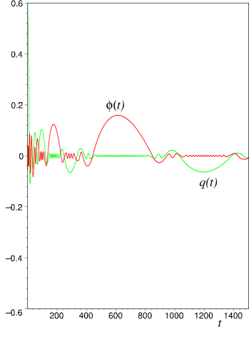
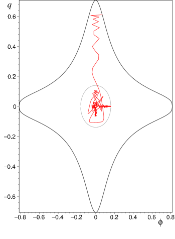
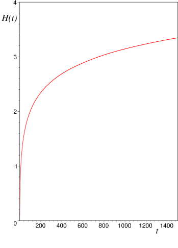
Figure 1: Typical behavior of a solution of the equations of motion (6) and (7) within an expanding universe. The upper left diagram shows the evolution of $\phi(t),q(t)$ with respect to cosmological time. For $0\lesssim t\lesssim 100$ and $1050\lesssim t\lesssim 1150$ the trajectory runs along the Higgs branch while for $550\lesssim t\lesssim 700$ it evolves along the Coulomb branch, indicating that the solution undergoes several conifold transitions. The upper right diagram displays the same trajectory projected to the $\phi$-$q$-plane. Here the bold black line illustrates the initial energy of the scalar fields while the gray circle illustrates our choice of the central region around the conifold point $\phi=q=0$. After the initial approach the trajectory gets trapped in this region. The lower left and lower right diagrams show the Hubble parameter $H(t)$ and the acceleration parameter $Q(t)$, respectively.

Looking at the time-dependence of $\phi(t),q(t)$ (upper left diagram) we observe that, analogous to the 5d case, conifold transitions are realized dynamically. Indeed, taking the order parameter for the transition to be $\xi(t):=|q(t)|/|\phi(t)|$ and adopting the criterion $\xi(t)\geq 100$ ($\xi(t)\leq 0.01$) for the solution to evolve along the Higgs (Coulomb) branch, the solution shows multiple transitions between these branches. Projecting the solution to the $\phi$-$q$-plane in the upper right diagram we see that it gets trapped in the vicinity of the conifold point at $\phi=q=0$. Analogous to the 5d case, this trapping is caused by an interplay between Hubble friction and the shape of the scalar potential which always pushes the solution back to the central region. In the 4d case the Hubble friction is slightly less effective due to the decreased numerical factor in front of the Hubble friction terms $\dot{\alpha}\dot{q}$ and $\dot{\alpha}\dot{\phi}$.

The lower left diagram shows that $H(t)$ increases monotonically in time. After a period of rapid increase ($0\leq t\leq 300$, say) its numerical value approaches a plateau value for late times. The numerical value of this plateau depends on the particular initial conditions chosen but typically gives $H_{\rm Plateau}\approx 3$. The acceleration parameter (lower right diagram) oscillates rapidly between $-1\leq Q(t)\leq 2$. The diagram thereby shows a number of short periods of accelerated expansion (corresponding to $Q(t)<0$) which, however, are not pronounced enough to give rise to a significant expansion of the space-time. Our results are consistent with what one expects from existing work on cosmological solutions in the vicinity of flop or conifold transitions [9, 14, 15, 13].

References

- [1] L. Kofman, A. Linde, X. Liu, A. Maloney, L. McAllister, E. Silverstein, JHEP 05 (2004) 030 [arXiv:hep-th/0403001].
- [2] B.R. Greene, in Fields, strings and duality, Boulder (1996) 543 [arXiv:hep-th/9702155].
- [3] A. Strominger, Nucl. Phys. B 451 (1995) 96 [arXiv:hep-th/9504090].
- [4] E. Witten, Nucl. Phys. B 471 (1996) 195 [arXiv:hep-th/9603150].
- [5] T. Mohaupt, M. Zagermann, JHEP 12 (2001) 026 [arXiv:hep-th/0109055].
- [6] T. Mohaupt, Fortsch. Phys. 51 (2003) 787 [arXiv:hep-th/0212200].
- [7] J. Louis, T. Mohaupt, M. Zagermann, JHEP 02 (2003) 053 [arXiv:hep-th/0301125].
- [8] S. Watson, Phys. Rev. D 70 (2004) 066005 [arXiv:hep-th/0404177]; Stabilizing moduli with string cosmology, arXiv:hep-th/0409281.
- [9] M. Brändle, A. Lukas, Phys. Rev. D 68 (2003) 024030 [arXiv:hep-th/0212263].
- [10] L. Järv, T. Mohaupt, F. Saueressig, JHEP 12 (2003) 047 [arXiv:hep-th/0310173].
- [11] T. Mohaupt, F. Saueressig, Effective supergravity actions for conifold transitions, [arXiv:hep-th/0410272].
- [12] F. Saueressig, Topological phase transitions in Calabi-Yau compactifications of M-theory, Ph.D. Thesis, Fortschr. Phys. 53 (2005) 5.
- [13] A. Lukas, E. Palti, P.M. Saffin, Type IIB conifold transitions in cosmology, arXiv:hep-th/0411033.
- [14] L. Järv, T. Mohaupt, F. Saueressig, JCAP 02 (2004) 012 [arXiv:hep-th/0310174]; ibid, in “Symmetries beyond the standard model”, Portoroz (2003) 254 [arXiv:hep-th/0311016].
- [15] T. Mohaupt, F. Saueressig, Dynamical conifold transitions and moduli trapping in M-theory cosmology, arXiv:hep-th/0410273.
- [16] H. Ooguri, C. Vafa, Phys. Rev. Lett. 77 (1996) 3296 [arXiv:hep-th/9608079].
- [17] T. Hübsch, Calabi-Yau manifolds, World Scientific, 1992.