LPTENS-05/05

Paperclip at $\theta=\pi$

Sergei L. Lukyanov^1,2, Alexei M. Tsvelik³

and

Alexander B. Zamolodchikov^1,2,4

¹ NHETC, Department of Physics and Astronomy

Rutgers University

Piscataway, NJ 08855-0849, USA

² L.D. Landau Institute for Theoretical Physics

Chernogolovka, 142432, Russia

³ Department of Physics, Brookhaven National Laboratory

Upton, NY 11973-5000, USA

and

⁴ Chaire Internationale de Recherche Blaise Pascal

Laboratoire de Physique Th${\acute{\rm e}}$orique de l’Ecole Normale Sup${\acute{\rm e}}$rieure

24 rue Lhomond, Paris Cedex 05, France

Abstract

We study the “paperclip” model of boundary interaction with the topological angle $\theta$ equal to $\pi$. We propose exact expression for the disk partition function in terms of solutions of certain ordinary differential equation. Large distance asymptotic form of the partition function which follows from this proposal makes it possible to identify the infrared fixed point of the paperclip boundary flow at $\theta=\pi$.

 

January 2005

Field theory models where interactions emerge as a consequence of geometric constrains imposed on the fields are much interest. They are esthetically attractive, and they often have rich content and important applications. Typical models of this class are nonlinear sigma models where the constraints are imposed in the bulk of the space-time. Lately the other type of models, where the constraints are imposed only on a boundary, attracts much attention. Two-dimensional models of this type emerge naturally in string theories and in some condensed matter problems. In string theories they provide the world-sheet description of “branes”, while in condensed matter theory they describe either quantum impurities or “quantum dots”.

In this paper we study one model of this type. It is the so-called paperclip model introduced in [1]. This two-dimensional model of quantum field theory involves two-component Bose field ${\bf X}(z,{\bar{z}})=\big{(}X(z,{\bar{z}}),Y(z,{\bar{z}})\big{)}$ living on the disk of radius $R$. In the bulk, i.e. at $|z|<R$, the field ${\bf X}(z,{\bar{z}})$ is a free massless field, as described by the bulk action

$${\cal A}_{\rm bulk}[{\bf X}]={1\over\pi}\,\int_{|z|<R}\mbox{d}^{2}z\ \,\partial_{z}{\bf X}\cdot\partial_{\bar{z}}{\bf X}\,,$$ (1)

while the boundary values ${\bf X}_{B}$ of this field, ${\bf X}_{B}={\bf X}|_{|z|=R}$, are subjected to a nonlinear constraint

$$r\,\cosh\big{(}{\textstyle{X_{B}\over\sqrt{n}}}\big{)}-\cos\big{(}{\textstyle{Y_{B}\over\sqrt{n+2}}}\big{)}=0\,,\ \ \qquad|Y_{B}|\leq{\pi\over 2}\,\sqrt{n+2}\ .$$ (2)

Here $n$ and $r$ are real and positive parameters (despite the notation, $n$ is not necessarily integer). The renormalization does not affect the parameter $n$, which is thus a scale-independent constant, while $r$ “flows” under the RG transformations; up to two loops, the flow is described by the equation

$$\kappa=(n+1)\ (1-r^{2})\,r^{n}\ ,$$ (3)

where $\kappa=\textstyle{E_{*}\over E}$ is inversely proportional to the RG energy scale $E$. Here $E_{*}$ is the integration constant of the RG equation, which sets up the “physical scale” in the model. As in [1], we will always choose $E$ equal to $R^{-1}$, the inverse radius of the disk, so that

$$\kappa=E_{*}R\,.$$ (4)

The equation (2) defines a closed curve in the $(X_{B},Y_{B})$ plane, which at sufficiently small $r$ has a paperclip shape (see Fig. 1), hence the name of the model.

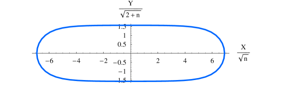
Figure 1: The paperclip shape for $r=2\times 10^{-3}$.

When $n$ goes to infinity and simultaneously $r$ goes to $1$ as $r=1-{1\over{2(n+1)g}}$ with finite $g$, the paperclip curve becomes a circle

$$X_{B}^{2}+Y_{B}^{2}={{1\over g}}\ ,$$ (5)

and the flow equation (3) reduces to

$$\kappa=g^{-1}\ \mbox{e}^{-{1\over{2g}}}\ .$$ (6)

The boundary constraint (5) defines the “circular brane” model [2].

The “circular brane” model has important application in condensed matter physics. It is equivalent to the model of dissipative quantum mechanics known as Ambegaokar-Eckern-Schön model [3]. The latter is used to describe the low-energy sector of the model of a “weakly blockaded” quantum dot introduced in [4, 5] (see also the review article [6]). That model describes an almost open dot which has a large number of energy levels and a large charging energy. The dot is connected to the bulk via $n$ degenerate channels, and the Ambegaokar-Eckern-Schön model applies when the number of channels is very large. In this application the circumference $2\pi R$ of the disk in (1) has obvious interpretation as the inverse temperature $1/T$, while the large charging energy provides explicit ultraviolet cut-off for the model, and the topological angle of the circular brane (introduced later in the text) is related to the gate voltage. Although the Ambegaokar-Eckern-Schön model appears only in the $n\to\infty$ limit of the model (2) when the paperclip becomes the circle (5), we have reasons to believe that the paperclip model with finite integer $n$ has certain relation to the quantum dot model with $n$ open degenerate channels. We intend to explore this possible relation in separate work.

The primary object of interest is the boundary state $|\,B\,\rangle$, in particular its overlap with the Fock vacuum $|\,{\bf P}\,\rangle$ characterized by the zero-mode momentum ${\bf P}=(P,Q)$ of the free field ${\bf X}=(X,Y)$. The overlap

$$\langle\,{\bf P}\,|\,B\,\rangle=Z(\,{\bf P}\,|\,\kappa\,)$$ (7)

can be expressed through the disk one-point function

$$R^{1/3-{{\bf P}^{2}/2}}\ Z(\,{\bf P}\,|\,\kappa\,)=\big{\langle}\,\mbox{e}^{\mbox{i}{\bf P}\cdot{\bf X}}(0,0)\,\big{\rangle}_{\rm disk}=\int\,{\cal D}{\bf X}\ \mbox{e}^{\mbox{i}\,{\bf P}\cdot{\bf X}(0,0)}\ \mbox{e}^{-{\cal A}_{\rm bulk}[{\bf X}]}\,,$$ (8)

where the functional integration is over all fields ${\bf X}(z,{\bar{z}})$ obeying the boundary constraint (2).

Let us repeat again that Eq. (3), as well as the paperclip equation (2), was obtained perturbatively, in the two-loop approximation. Therefore it provides useful description of the boundary condition only in the weak coupling regime, where the curvature of the paperclip curve (2) is small everywhere; this requires $n$ to be large, $n\gg 1$, and $r$ to be sufficiently small (so that $r^{n}\ll 1$); according to (3), the last condition is fulfilled at sufficiently small $R$, therefore Eqs. (2), (3) provide ultraviolet (UV) description of the boundary condition. At large distances (large $R$) and at $n\sim 1$ the higher loops and non-perturbative corrections are important. Generally, one expects that at $R\to\infty$ the paperclip boundary theory “flows” to some infrared (IR) fixed point, and so the $R=\infty$ limit of the boundary state $|\,B\,\rangle$ is described in terms of conformal boundary theory associated with the IR fixed point.

In regard to the non-perturbative effects, it is important to realize that under general definition the paperclip model may involve an additional parameter, the topological angle $\theta$. Since topologically the paperclip curve (2) is a circle, the configuration space for the field ${\bf X}(z,{\bar{z}})$ consists of topological sectors, each characterized by integer $w$ which is the number of times the boundary value ${\bf X}_{B}$ winds around the paperclip curve when one goes around the disk boundary $|z|=R$. This allows one to add the weight factors $\mbox{e}^{{\rm i}w\theta}$ to all contributions to the functional integral coming from the sectors with the winding number $w$. Thus, in general

$$Z(\,{\bf P}\,|\,\kappa\,)=\sum_{w=-\infty}^{\infty}\mbox{e}^{{\rm i}w\theta}\ Z^{(w)}(\,{\bf P}\,|\,\kappa\,)\,,$$ (9)

where $Z^{(w)}$ receives contributions from the topological sector $w$ only. Of course, the contributions of the instanton sectors $w\neq 0$ are invisible in the perturbation theory, and therefore the UV limit $R\to 0$ of the theory is insensitive to the topological angle (this statement is not limited to the case $n\gg 1$; the instanton contributions are suppressed by the powers of $\kappa$ at any $n$, see [1]). However, the IR behavior of the theory can depend on $\theta$ in a significant way.

The paperclip model is in a close analogy with the so called “sausage” sigma model proposed and studied in [7] (perhaps better known is the symmetric limit of the sausage model, that $O(3)$ nonlinear sigma model; its counterpart is the circular brane model (5)). The IR physics of the sausage (and its $O(3)$ limit) sigma model strongly depends on its topological angle $\theta$ [8, 9]. The sausage sigma model is believed to be integrable at two values of the topological angle, $\theta=0$ and $\theta=\pi$. The arguments were given in [7], where exact solutions of the sausage model at these two values of $\theta$ were proposed. According to this proposal, the sausage model at $\theta=0$ is massive and its solution is described in terms of factorizable $S$-matrix of three massive particles. On the contrary, the sausage model at $\theta=\pi$ “flows” in the IR limit to a critical fixed point, which is the $c=1$ CFT of a compactified free boson; the “flow” is described in terms of certain massless Thermodynamic Bethe Ansatz (TBA) system [7]. Solutions for the $O(3)$ sigma model at $\theta=0$ and $\theta=\pi$ were previously proposed in [10] and [11]. By the analogy, one may expect that the paperclip model is also integrable in two cases $\theta=0$ and $\theta=\pi$.

There is more then just this analogy to suspect that the paperclip model might be integrable at least at some values of $\theta$. In [1] a set of commuting local integrals of motion $\{\,{\mathbb{I}}_{2l-1}\,\}_{l=1}^{\infty}$ of the free Bose theory (1) was displayed which has all symmetries of the paperclip (2), and moreover it was found that given the symmetries the set is essentially unique. The idea that this series has something to do with the paperclip model can be supported by the analysis of the UV properties of the model. In the UV limit $R\to 0$ the parameter $r$ in (2) becomes small, and the paperclip grows long in the $X$ direction; in this limit the paperclip can be regarded as the composition of left and right “hairpins” (see Fig. 2).

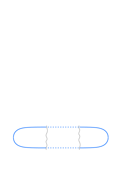
Figure 2: The paperclip formed by a junction of two hairpins.

By the “hairpins” we understand the curves

$${\textstyle{r\over 2}}\ \exp\big{(}\pm{\textstyle{X_{B}\over\sqrt{n}}}\big{)}=\cos\big{(}{\textstyle{Y_{B}\over\sqrt{n+2}}}\big{)}\ ,$$ (10)

where the sign plus (minus) has to be taken for the left (right) hairpin. If any one of the curves (10) is taken as the boundary constraint, the associated left and right “hairpin models” are conformally invariant, and moreover each has extended conformal symmetry with respect to certain $W$-algebra [1]. Although the $W$-algebras of the right and left hairpin models are isomorphic, the generators of $W^{(\subset)}$ and $W^{(\supset)}$ are realized by different operators in the space of states of the free boson theory (1). However, the sets of operators $W^{(\subset)}$ and $W^{(\supset)}$ have nontrivial intersection, which is exactly the set of commuting integrals $\{{\mathbb{I}}_{2l-1}\}$  [1]. For these reasons we refer to the set $\{{\mathbb{I}}_{2l-1}\}$ as the “paperclip series” of local IM.

In [1] an exact expression for the amplitude $Z_{\theta=0}(\,{\bf P}\,|\,\kappa\,)$ was proposed in terms of solutions of certain linear differential equation. The proposal was inspired by remarkable observation of Dorey and Tateo [12] who found that in somewhat simpler integrable model of boundary interaction (the minimal CFT with non-conformal boundary perturbation) the overlap amplitude analogous to (7) is related to certain monodromy coefficients of the Schr$\rm{\ddot{o}}$edinger equation with the potential $|x|^{2\alpha}$. Since [12], this finding was confirmed and extended to several other integrable models of boundary interaction [13, 14, 15]. Although it is fair to say that true roots of this relation remain mysterious to us, the examples suggest that the relation may be rather general. Given a model of boundary interaction suspect of being integrable, it is worth trying to identify associated ordinary differential equation. The proposal of [1] was made according to this strategy. Let us briefly summarize it here.

The main ingredient is the ordinary differential equation

$$\bigg{[}-{{\mbox{d}^{2}}\over{\mbox{d}x^{2}}}-{\textstyle{nP^{2}\over 4}}\,{{\mbox{e}^{x}}\over{1+\mbox{e}^{x}}}-{\textstyle{(n+2)Q^{2}-1\over 4}}\,{{\mbox{e}^{x}}\over{(1+\mbox{e}^{x})^{2}}}+\kappa^{2}\,\big{(}1+\mbox{e}^{x}\big{)}^{n}\bigg{]}\,\Psi(x)=0\,,$$ (11)

where $P$ and $Q$ are the $X$ and $Y$ components of the zero-mode momentum ${\bf P}$, and $\kappa$ is the same as in (4); according to the definition (4) we assume for the moment that $\kappa$ is real and positive.

Eq. (11) has a form of a stationary zero energy Schr${\rm\ddot{o}}$edinger equation with specific potential $V(x)$ given by the last three terms in (11). The potential $V(x)$ is positive and grows fast at large positive $x$, therefore (11) has a solution $\Xi(x)$ decaying at $x\to+\infty$; this condition specifies $\Xi(x)$ uniquely up to normalization. To fix the normalization, we assume that

$$\Xi(x)\to\kappa^{-{1\over 2}}\ \exp\bigg{\{}-\big{(}{\textstyle{n\over 4}}+\kappa\big{)}\,x-\kappa\,\int_{0}^{\mbox{e}^{x}}{\mbox{d}u\over u}\,\big{(}(1+u)^{n\over 2}-1\big{)}\,\bigg{\}}$$ (12)

as $x\to+\infty$. On the other hand, $V(x)$ approaches positive constant $\kappa^{2}$ at large negative $x$. Hence Eq. (11) has a solution which decays at large negative $x$; we denote this solution $\Psi_{+}(x)$. The condition,

$$\Psi_{+}(x)\to{{\mbox{e}^{\kappa x}}\over{\Gamma(1+2\kappa)}}\quad{\rm as}\quad x\to\infty\,,$$ (13)

specifies the solution $\Psi_{+}(x)$ uniquely, including its normalization. Then

$$Z_{\theta=0}(\,{\bf P}\,|\,\kappa\,)={\rm g}_{D}^{2}\,\sqrt{\pi}\ \Big{(}{{2\kappa}\over\mbox{e}}\Big{)}^{2\kappa}\,W\big{[}\Xi,\Psi_{+}\big{]}\,.$$ (14)

Here and below ${\rm g}_{D}=2^{-1/4}$ is the $g$-factor [16] of the Dirichlet boundary, and $W[F,G]$ denotes the Wronskian $F(x)G^{\prime}(x)-F^{\prime}(x)G(x)$. Eq. (14) is the proposal of [1].

It was shown in [1] that (14) exhibits the UV (i.e $\kappa\to 0$) behavior completely consistent with what one expects from the “hairpin decomposition” of the paperclip at $R\to 0$. At small $\kappa$ the expression (14) can be written as (here we write explicitly the components of ${\bf P}=(P,Q)$)

$$Z_{\theta=0}(\,P,Q\,|\,\kappa\,)=B(P,Q)\ F_{\theta=0}(P,Q\,|\,\kappa)+B(-P,Q)\ F_{\theta=0}(-P,Q\,|\,\kappa)\,,$$ (15)

where

$$B(P,Q)={\rm g}_{D}^{2}\ \Big{(}{\kappa\over n}\Big{)}^{\mbox{i}{P\over\sqrt{n}}}\times$$ (16)

$$\ \ \ \ {{\sqrt{n}\ \Gamma(-\mbox{i}\sqrt{n}\,P)\,\Gamma(1-{{\mbox{i}P}/\sqrt{n}})}\over{\Gamma\big{(}{1\over 2}-\sqrt{n+2}\ {Q\over 2}-\mbox{i}\sqrt{n}\ {P\over 2})\,\Gamma\big{(}{1\over 2}+\sqrt{n+2}\ {Q\over 2}-\mbox{i}\sqrt{n}\ {P\over 2}\big{)}}}\ ,$$

and $F_{\theta=0}(P,Q\,|\,\kappa)$ (apart from the factor $\kappa^{2\kappa}$) admits asymptotic expansion in a double series in powers of $\kappa$ and $\kappa^{2\over n}$ (here and below we use the symbol $\simeq$ to indicate relations which hold in the sense of asymptotic series),

$$F_{\theta=0}(P,Q|\kappa)\simeq\kappa^{2\kappa}\,\sum_{i,j=0}^{\infty}\,f_{i,j}(P,Q)\,\kappa^{i+{{2j}\over n}}\,,$$ (17)

with $f_{0,0}=1$. From (14), the powers $\kappa^{2\over n}$ appear from the $\kappa\to 0$ expansion of the solution $\Xi(x)$, while the integer powers of $\kappa$ come from the expansion of $\Psi_{+}(x)$.

The expansion (15) is in good agreement with expected form of (8) in the domain $\kappa\ll 1$. Recall that according to (4) and (3) this domain corresponds to the UV limit of the paperclip model, where the paperclip (2) can be regarded as the composition of two hairpins, as in Fig. 2. Roughly speaking, the two terms in (15) correspond to contributions from the right and the left hairpins, respectively. More precisely, at small $\kappa$ and $\Im m\,P\neq 0$ the saddle points of the functional integral (8) correspond to the field configurations where the boundary values $(X_{B},Y_{B})$ are mostly concentrated near the left or the right end of the paperclip (2). The factors $B(P,Q)$ and $B(-P,Q)$ are precisely the boundary overlap amplitudes of the right and left hairpin models (10), respectively. The powers of $\kappa^{2\over n}$ in (17) are associated with the perturbative corrections, due to “small” fluctuations around the saddle points, which feel only the small deviations of the shape of the paperclip (2) from the respective hairpin, while the integer powers of $\kappa$ are associated with the contributions of the $w\neq 0$ topological sectors in (9) (see Ref. [1] for more detailed discussion, which also includes the explanation of the factor $\kappa^{2\kappa}$ in (14) and (17) as the effect of small instantons).

On the other hand, when $\kappa\to\infty$ (and $P,Q$ are fixed) the potential term in (11) becomes large at all real $x$, and therefore the Wronskian in (14) can be found by straightforward application of WKB technique. This results in the asymptotic $\kappa\to\infty$ series

$$Z_{\theta=0}(\,{\bf P}\,|\,\kappa\,)\simeq{\rm g}_{D}^{2}\ \exp\bigg{\{}-\sum_{l=1}^{\infty}\,{{I_{2l-1}({\bf P})}\over{\kappa^{2l-1}}}\,\bigg{\}}\,,$$ (18)

where $I_{2l-1}({\bf P})=I_{2l-1}(P,Q)$ are certain polynomials in $P^{2},$ and $Q^{2}$ of the degree $l$, with coefficients which depend only on $n$. It turns out that these polynomials are exactly the vacuum eigenvalues of the local IM of the “paperclip series” $\{{\mathbb{I}}_{2l-1}\}$,

$${\mathbb{I}}_{2l-1}\ |\,{\bf P}\,\rangle=R^{1-2l}\ {I_{2l-1}(P,Q)}\ |\,{\bf P}\,\rangle$$ (19)

(see [1] for details). This form of IR expansion suggests that at $\theta=0$ the IR fixed point is just the Dirichlet boundary condition for the free field ${\bf X}=(X,Y)$:

$$(X_{B},Y_{B})=(0,0)\,.$$ (20)

According to (18) the RG flow approaches the Dirichlet fixed point along irrelevant direction which is a combination of densities of the paperclip IM $\{{\mathbb{I}}_{2l-1}\}$.

In this paper we extend the proposal of [1] to the case $\theta=\pi$. The starting point is the same differential equation (11), but now instead of $\Psi_{+}$ in (14), we take another solution which grows as $\mbox{e}^{-\kappa x}$ at large negative $x$. Of course, this condition alone does not define the solution uniquely since, besides overall normalization, one can always add any amount of $\Psi_{+}(x)$. Usually it is difficult to make unambiguous definition of a growing solution, but in our case the following property of (11) helps. Let us consider $x$ as a complex variable. The potential $V(x)$ is analytic function of $x$ with the branching-point singularities at all points where $\mbox{e}^{x}$ turns to $-1$. Let us make brunch cuts from each of the points $x=\pi\mbox{i}\,(2N+1)$, $N=0,\pm 1,\pm 2,\ldots$ to $+\infty$ parallel to the real axis, and choose the branch of $V(x)$ on which $(1+\mbox{e}^{x})^{n}$ is real and positive on the real axis of the $x$-plane. Now, restricting attention to the domain $\Re e\,x<0$ one finds that the potential $V(x)$ has the periodicity property

$$V(x+2\pi\mbox{i})=V(x)\qquad(\Re e\,x<0)\,.$$ (21)

Consequently, the equation (11) has two Bloch-wave solutions ($2\kappa\not\in{\mathbb{Z}}$):

$$\Psi_{\pm}(x+2\pi\mbox{i})=\mbox{e}^{\pm 2\pi{\rm i}\,\kappa}\,\Psi_{\pm}(x)\ \ \qquad(\Re e\,x<0)\,,$$ (22)

where the Bloch factors are found by taking the limit $\Re e\,x\to-\infty$. At this point we assume that $2\kappa$ is not an integer, so that the conditions (22) specify the two independent solutions $\Psi_{\pm}(x)$ uniquely, up to their normalizations. Of course, the solution $\Psi_{+}(x)$ defined this way decays as $\mbox{e}^{\kappa x}$ at $\Re e\,x\to-\infty$, and the asymptotic condition  (13) also fixes its normalization. The solution $\Psi_{-}(x)$ grows at large negative $\Re e\,x$, and its normalization can be fixed by specifying the leading asymptotic in this domain. Thus we define $\Psi_{-}(x)$ by the conditions

$$\Psi_{-}(x+2\pi\mbox{i})=\mbox{e}^{-2\pi{\rm i}\,\kappa}\,\Psi_{-}(x)\quad(\Re e\,x<0)\,,$$ (23)

$$\Psi_{-}(x)\to{{\mbox{e}^{-\kappa x}}\over{\Gamma(1-2\kappa)}}\ \ \ \ \quad{\rm as}\quad\ \ \ \ \Re e\,x\to-\infty\,.$$

It is possible to show that both $\Psi_{+}(x)$ and $\Psi_{-}(x)$ defined by  (13) and  (23) are entire functions of $\kappa$, and

$$\Psi_{-}(\kappa\,|\,x)=\Psi_{+}(-\kappa\,|\,x)\,,$$ (24)

where we temporarily exhibited the dependence of $\Psi_{\pm}$ of the parameter $\kappa$. From the definitions (13) and (23) we have

$$W\big{[}\Psi_{-},\Psi_{+}\big{]}={{\sin(2\pi\kappa)}\over{\pi}}\,.$$ (25)

Our proposal for $Z_{\theta=\pi}$ is

$$Z_{\theta=\pi}(\,{\bf P}\,|\,\kappa)={\rm g}_{D}^{2}\,\sqrt{\pi}\ \Big{(}{{2\kappa}\over\mbox{e}}\Big{)}^{-2\kappa}\,W\big{[}\Xi,\Psi_{-}\big{]}\,.$$ (26)

The $\kappa\to 0$ form of the Wronskian in (26) can be derived through the perturbative evaluation of the solutions $\Xi(x)$ and $\Psi_{-}(x)$, as it was done in [1] for the Wronskian in  (14). This leads to the expansion similar to  (15),

$$Z_{\theta=\pi}(\,P,Q\,|\,\kappa\,)=B(P,Q)\ F_{\theta=\pi}(P,Q\,|\,\kappa)+B(-P,Q)\ F_{\theta=\pi}(-P,Q\,|\,\kappa)\,,$$ (27)

where $B(P,Q)$ is the same as in  (15), while

$$F_{\theta=\pi}(P,Q|\kappa)\simeq\kappa^{-2\kappa}\,\sum_{i,j=0}^{\infty}\,f_{i,j}(P,Q)\,(-\kappa)^{i}\,\kappa^{{{2j}\over n}}\,,$$ (28)

with exactly the same coefficients $f_{i,j}(P,Q)$ as in (17). This form follows from the fact that integer powers of $\kappa$ in (28) come from perturbative expansion of the solution $\Psi_{-}(x)$; in view of (24) they are related to corresponding integer powers in (17) by the change of the sign, $\kappa\to-\kappa$. At the same time, the powers of $\kappa^{2\over n}$ appear as the result of expansion of $\Xi(x)$, and hence they remain unchanged in (28) as compared to (17). Since the powers of $\kappa^{2\over n}$ are interpreted as the perturbative contributions to the functional integral (8), while the integer powers of $\kappa$ are due to the instanton contributions, the form (27), (28) is exactly what one expects to have from the definition (9) at $\theta=\pi$. This property of the UV expansion was the main motivation of our proposal (26).

Accepting (26), we can address the problem of the IR behavior of the paperclip model at $\theta=\pi$. One has to find the $\kappa\to\infty$ asymptotic of the Wronskian in (26). Unlike the case $\theta=0$, Eq. (14), this turns out to be rather subtle problem. While at $\kappa\to\infty$ the WKB approximation still formally applies to (11), the problem is analogous to the problem of finding the “over-the-barrier” reflection amplitude in quantum mechanics which in the semiclassical approximation requires identifying appropriate “turning points” (the zeroes of the potential $V(x)$) in the complex $x$-plane [17]. In our case, at large $\kappa$ all the complex turning points approach the singular points $\mbox{e}^{x}=-1$ where the semiclassical approximation for (11) breaks down. Finding correct $\kappa\to\infty$ expansion of (26) requires analysis of the solutions of (11) in the vicinities of the singular points $\mbox{e}^{x}=-1$. The calculations are rather involved, and will be present them elsewhere. The result is the asymptotic $\kappa\to\infty$ expansion

$$Z_{\theta=\pi}(\,{\bf P}\,|\,\kappa\,)\simeq{\rm g}_{D}^{2}\ \,\mbox{e}^{a\,\kappa}\ \,T(\,{\bf P}\,|\,\kappa)\ \exp\bigg{\{}\,\sum_{l=1}^{\infty}\,{{I_{2l-1}({\bf P})}\over{\kappa^{2l-1}}}\,\bigg{\}}\,,$$ (29)

where $a$ is a constant , $I_{2l-1}({\bf P})$ are the same eigenvalues of the “paperclip IM” ${\mathbb{I}}_{2l-1}$ as in (18), and $T(\,{\bf P}\,|\,\kappa\,)$ is the asymptotic series in inverse powers of $\kappa^{2\over{n+2}}$,

$$T(\,{\bf P}\,|\,\kappa\,)\simeq 2\cos\big{(}{\textstyle{\pi\,Q\over\sqrt{n+2}}}\big{)}+\sum_{l=1}^{\infty}t_{l}(P,Q)\ \kappa^{-{{2l}\over{n+2}}}\,.$$ (30)

Here again $P$ and $Q$ are the $X$ and $Y$ components of the zero-mode momentum, i.e. ${\bf P}=\big{(}P,Q)$, and the coefficients $t_{l}(P,Q)$ are in principle computable through perturbative solution of (11) in the vicinity of the singular points $\mbox{e}^{x}=-1$. The first two coefficients can be evaluated in closed form. We have

$$t_{1}(P,Q)=\bigg{(}{{n+2}\over 2}\bigg{)}^{2\over{n+2}}\,{{\Gamma\big{(}{1\over 2}-{1\over{n+2}}\big{)}}\over{\sqrt{\pi}\,\Gamma\big{(}1-{1\over{n+2}}\big{)}}}\,\times$$ (31)

$$\bigg{[}{{n+2}\over{n+4}}-{{(n+2)\,Q^{2}-n\,P^{2}-1}\over{2\,((n+2)\,Q^{2}-1)}}\bigg{]}\,{{2\,\pi^{2}}\over{\Gamma\big{(}{Q\over\sqrt{n+2}}-{1\over{n+2}}\big{)}\,\Gamma\big{(}-{Q\over\sqrt{n+2}}-{1\over{n+2}}\big{)}}}\,,$$

while the expression for $t_{2}(P,Q)$ is somewhat cumbersome, and we present it in Appendix.

The most important difference of  (29) from (18) is in the factor (30) which involves the powers of ${\kappa^{-{2\over{n+2}}}}$; its presence indicates that in this case the IR fixed point differs from the trivial Dirichlet boundary constraint (20). The series (30) starts with the term $2\cos\big{(}{\textstyle{\pi\,Q\over\sqrt{n+2}}}\big{)}$ which suggests that in the limit $\kappa\to\infty$ the boundary values of ${\bf X}$ are constrained to two points,

$$(X_{B},Y_{B})=\big{(}0,\pm{\textstyle{\pi\over\sqrt{n+2}}}\big{)}\,.$$ (32)

Eq. (32) characterizes the IR fixed point of the paperclip boundary flow at $\theta=\pi$. At large but finite $\kappa$ the boundary value $\big{(}X_{B},Y_{B}\big{)}$ is allowed to jump between the two points (32), the possibility of such jumps being responsible for the higher-order terms in the series (30). In other words, the RG flow arrives at the IR fixed point (32) along certain irrelevant boundary fields which generate such jumps. Obvious candidates are the boundary vertex operators

$$V_{\pm}(\tau)=[\partial_{\sigma}X]_{B}\ \mbox{e}^{\pm{{{\rm i}\,{\tilde{Y}}_{B}}\over\sqrt{n+2}}}(\tau)\,,$$ (33)

where $\tau$ is natural coordinate along the boundary (we write $z/R=\mbox{e}^{{\sigma+{\rm i}\tau}\over R}$, so that the boundary $|z|=R$ is at $\sigma=0$), $[\partial_{\sigma}X]_{B}=\partial_{\sigma}X(\sigma,\tau)|_{\sigma=0}$ is the normal derivative of the field $X$ at the boundary, and ${\tilde{Y}}_{B}(\tau)$ is the boundary value of ${\tilde{Y}}$, the T-dual of $Y$ . The exponentials $\exp\big{(}{\pm{{\mbox{i}\,{\tilde{Y}}_{B}}\over\sqrt{n+2}}}\big{)}(\tau)$ create jumps in the boundary value $Y_{B}$ at the point $\tau$, i.e. the boundary values $Y_{B}$ to the right and to the left of each vertex $V_{\pm}(\tau)$ differ by the amount $\pm{2\pi\over\sqrt{n+2}}$. Note that the dimensions of the fields (33) equal to $1+{1\over{n+2}}$, which is in exact agreement with the fractional power $\kappa^{-{2\over{n+2}}}$ appearing in the expansion (30). According to these arguments, it seems likely that the full asymptotic series (30) can be generated by expanding the following expression

$$\ \ \ \ \ \ \ T(\,{\bf P}\,|\,\kappa\,)=$$ (34)

$$\big{\langle}\,{\bf P}\,\big{|}\,{\rm Tr}\Big{[}\mbox{e}^{{{{\rm i}\pi Q}\over{\sqrt{n+2}}}\,\sigma_{z}}\ {\cal T}\exp\Big{\{}\lambda\int_{0}^{2\pi R}\mbox{d}\tau\,\big{(}\sigma_{-}V_{+}(\tau)+\sigma_{+}V_{-}(\tau)\big{)}\Big{\}}\Big{]}\,\big{|}\,B_{D}\,\big{\rangle}\,.$$

Here $|\,B_{D}\,\rangle$ is the boundary state of the free theory (1) with the Dirichlet boundary condition (20) which is the superposition $|\,B_{D}\,\rangle=\int\,\mbox{d}^{2}{\bf P}\ |\,I_{\bf P}\,\rangle$ of the Dirichlet Ishibashi states $|\,I_{\bf P}\,\rangle$. In what follows we assume that the exponentials in (33) are normalized in such a way that

$$\langle\,{\bf P}\,|\,V_{+}(\tau)V_{-}(\tau^{\prime})\,|\,B_{D}\,\rangle\to 2\ |\tau-\tau^{\prime}|^{-2-{2\over{n+2}}}\quad{\rm as}\quad\tau-\tau^{\prime}\to 0\,.$$ (35)

The $\tau$-ordered exponential is understood in terms of its expansion in powers of the parameter $\lambda$ (which will be related to the parameter $E_{*}$, see Eq. (37) below),

$$T(\,{\bf P}\,|\,\kappa\,)=2\cos\big{(}{\textstyle{\pi\,Q\over\sqrt{n+2}}}\big{)}+{\textstyle{{\lambda^{2}}\over 2}}\ \int_{0}^{2\pi R}\mbox{d}\tau\int_{0}^{\tau}\mbox{d}\tau^{\prime}\times$$ (36)

$$\ \ \ \ \big{\langle}\,{\bf P}\,\big{|}\,\Big{[}\,\mbox{e}^{-{{{\rm i}\pi Q}\over{\sqrt{n+2}}}}\ V_{+}(\tau)\,V_{-}(\tau^{\prime})+\mbox{e}^{{{{\rm i}\pi Q}\over{\sqrt{n+2}}}}\ V_{-}(\tau)\,V_{+}(\tau^{\prime})\,\Big{]}\,\big{|}\,B_{D}\,\big{\rangle}+\ldots\,.$$

The relations $\sigma_{\pm}^{2}=0$ guarantee that the boundary values of $Y$ are limited to two points indicated in (32). With this understood, two eigenstates of $\sigma_{z}$ with the eigenvalues $\pm 1$ appear to be in correspondence with two possible boundary values $Y_{B}=\pm{\pi\over\sqrt{n+2}}$. At the same time, the $\sigma$-matrices in (34) can be regarded as operators representing an additional boundary degree of freedom; then the expression in the exponential in (34) is interpreted as the boundary action describing perturbation of the Dirichlet boundary condition. Anyhow, the $g$-factor at the IR fixed point (i.e. (29) evaluated at $\kappa=\infty$ and ${\bf P}=0$) is $2\,{\rm g}_{D}^{2}$, not ${\rm g}_{D}^{2}$ as it was in the case of the $\theta=0$ IR fixed point (20).

As was mentioned above, the dimensions of the vertex operators (33) are greater than one. As the result, the integrals appearing in the expansion (36) generally diverge when $\tau$-separations between the insertions $V_{\pm}(\tau)$ become small. One has to specify some regularization to make the expression (34) meaningful. We assume here the “analytic regularization” common in conformal perturbation theory. The prescription is to consider $n$ as an arbitrary complex number and to evaluate the integrals in the domain of $n$ where they converge (specifically, at $\Re e\,n<-4$), and then to continue in $n$ to the real positive values. It turns out that this continuation yields unique finite results for all integrals involved in the expansion (36). Thus, the $\lambda^{2}$ term explicitly written in (36) is readily evaluated in analytic form. Remarkably, its dependence of the momenta $(P,Q)$ appears exactly the same as in (31), and upon identification

$$\lambda={{\sqrt{n}}\over{\sqrt{2}\,\Gamma\big{(}-{1\over{n+2}}\big{)}}}\,\bigg{(}{{n+2}\over{E_{*}}}\bigg{)}^{1\over{n+2}}\ ,$$ (37)

it coincides with the first ($l=1$) term $t_{1}(P,Q)\,\kappa^{-{2\over{n+2}}}$ of the expansion (30). We believe that under the identification (37), and with the analytic regularization described above, the expression (34) reproduces all terms of the asymptotic series (30), i.e. it plays the role of the “effective IR theory” describing the approach of the $\theta=\pi$ paperclip flow to its IR fixed point (32). Note that the effective theory (34) is expected to capture only the “perturbative” part (30) of the full IR expansion (29), and it does not seem to have any control over the “nonperturbative” terms due to the local IM in (29).

The relation (37) is singular at $n=\infty$. Correspondingly, obtaining correct $n\to\infty$ limit from the effective theory (34) is not exactly straightforward. At $n\gg 1$ alternative form of the IR effective theory is more convenient. It is written as

$$\ \ \ \ \ \ T(\,{\bf P}\,|\,\kappa\,)=$$ (38)

$$\langle\,{\bf P}\,|\,{\rm Tr}\,{\cal T}\exp\Big{\{}\int_{0}^{2\pi R}\mbox{d}\tau\,\big{(}{\textstyle{{\alpha_{\rm x}}\over 2}}\ \sigma_{x}\,[\partial_{\sigma}X]_{B}(\tau)+{\textstyle{{\alpha_{\rm y}}\over 2}}\ \sigma_{y}\,[\partial_{\sigma}Y]_{B}(\tau)\big{)}\Big{\}}\,|\,B_{D}\,\rangle\,,$$

where again $[\partial_{\sigma}X]_{B}$ and $[\partial_{\sigma}Y]_{B}$ are the normal derivatives of the fields $X$ and $Y$ at the boundary, and $\alpha_{\rm x}$, $\alpha_{\rm y}$ are coupling constants. Formally, (38) can be brought to the form (34) by field-dependent gauge transformation

$$\sigma_{\rm a}\to\mbox{e}^{-{{{\rm i}\alpha_{\rm y}}\over 2}\,\sigma_{\rm y}{\tilde{Y}}_{B}}(\tau)\ \sigma_{\rm a}\ \mbox{e}^{{{{\rm i}\alpha_{\rm y}}\over 2}\,\sigma_{\rm y}{\tilde{Y}}_{B}}(\tau)\ ,$$ (39)

with obvious relabeling of the $\sigma$-matrices to match the notations in (34). The subtlety in this transformation is in the renormalization of the parameters. Perturbation theory in the couplings $\alpha_{\rm x}$, $\alpha_{\rm y}$ in (38) has logarithmic UV divergences which lead to renormalization of these parameters. In view of the $X\leftrightarrow Y$ symmetry the corresponding RG flow equations can be written as

$$-E\ {\mbox{d}g_{\rm x}\over{\mbox{d}E}}=\beta(g_{\rm x},g_{\rm y})\,,\ \ \ -E\ {\mbox{d}g_{\rm y}\over{\mbox{d}E}}=\beta(g_{\rm y},g_{\rm x})\,,$$ (40)

where $E$ is the RG energy scale, and $g_{\rm x}=\alpha_{\rm x}^{2}$, $g_{\rm y}=\alpha_{\rm y}^{2}$. The model (38) was studied in [19], where the leading (one-loop) term of the beta-function is presented,

$$\beta(g_{\rm x},g_{\rm y})=-2\ g_{\rm x}g_{\rm y}+O(g^{3})\ .$$ (41)

The higher loop terms depend on the renormalization scheme. One can note that (34) is easily evaluated in the limit when $g_{\rm x}\to 0$ with $g_{\rm y}$ kept finite (or when $g_{\rm y}\to 0$ with finite $g_{\rm x}$). It follows from this solution that a class of “natural” schemes exists in which

$$\beta(g,0)=\beta(0,g)=0\,,\ \ \ {\mbox{d}\over{\mbox{d}g}}\,\beta(g,h)\big{|}_{g=0}=-2\,h\,.$$ (42)

In any such scheme

$$\beta(g_{\rm x},g_{\rm y})=-2\ g_{\rm x}g_{\rm y}+b\ g_{\rm x}^{2}g_{\rm y}+O(g^{4})\ ,$$ (43)

where the constant $b$ is scheme independent. Explicit two-loop calculation yields $b=4$. The terms $\sim g^{4}$ and higher still depend on the scheme. It looks likely that any RG flow equation of the form (40) with the $\beta$-function satisfying (42) and having the expansion (43) with $b=4$ can be brought, order by order in $g$, to the following convenient form

$$-E\ {\mbox{d}{\hat{g}}_{\rm x}\over{\mbox{d}E}}=-E\ {\mbox{d}{\hat{g}}_{\rm y}\over{\mbox{d}E}}=-{{2\,{\hat{g}}_{\rm x}{\hat{g}}_{\rm y}}\over{1+{\hat{g}}_{\rm x}+{\hat{g}}_{\rm y}}}\ ,$$ (44)

where ${\hat{g}}_{\rm x}=g_{\rm x}/(1-g_{\rm x})$, ${\hat{g}}_{\rm y}=g_{\rm y}/(1-g_{\rm y})$, by appropriate redefinition of the coupling constants $g_{\rm x}$, $g_{\rm y}$ (we have explicitly checked this statement up to the order $g^{6}$). The RG flow (44) conserves the difference $\epsilon={\hat{g}}_{\rm y}-{\hat{g}}_{\rm x}$. In the coordinates ${\hat{g}}_{\rm x},{\hat{g}}_{\rm y}$ the RG trajectories are straight lines which end at the IR fixed points $g_{\rm x}=0$ if $\epsilon>0$, or $g_{\rm y}=0$ if $\epsilon<0$. Let us assume here $\epsilon\geq 0$. The RG invariant $\epsilon$ can be related to the parameter $n$ in (34),

$$\epsilon\equiv{\hat{g}}_{\rm y}-{\hat{g}}_{\rm x}={1\over{n+1}}\ .$$ (45)

Indeed, at the IR fixed point ${g}_{\rm x}=0$ while $g_{\rm y}={\textstyle{\epsilon\over 1+\epsilon}}$; the last quantity must coincide with the dimension of the coupling constant $\lambda$ in (34). Integrating (44) one finds

$${\hat{g}}_{\rm x}={{\epsilon\,\rho}\over{1-\rho}}\,,\ \ \ \ {\hat{g}}_{\rm y}={{\epsilon}\over{1-\rho}}\,,$$ (46)

where $\rho$ decays towards IR according to the equation

$${{\epsilon\,\rho^{{1\over 2\epsilon}}}\over{1-\rho}}={{E\over E_{0}}}\ ,$$ (47)

where $E_{0}$ is the integration constant; one can set $E_{0}=C\,E_{*}$ with an arbitrary constant $C$. The equations (46), (47) define a family of $E$-dependent renormalized coupling constants ${\hat{g}}_{x},\ {\hat{g}}_{y}$. It is clear that (38) admits perturbative expansion in these coupling constants, and if one chooses $E=R^{-1}$ the coefficients of this series are undependent of $R$.

Let us consider the case $n=\infty$ which is of special interest because it corresponds to the circular brane model [2] at $\theta=\pi$, and hence is equivalent to the Ambegaokar-Eckern-Schön model [3] of quantum dot at the degeneracy point. Obviously, in this limit the form (30) of the IR asymptotic expansion of the boundary amplitude is no longer meaningful. Instead, in this case the factor $T(\,{\bf P}\,|\,\kappa\,)$ in (29) rather expands in powers the “running coupling constant” ${\hat{g}}$ related to $\kappa$ by the equation

$${\hat{g}}\ \mbox{e}^{-{1\over{2{\hat{g}}}}}={1\over{\mbox{e}^{c_{0}}\,\kappa}}\ .$$ (48)

The same relation is obtained by integrating the RG equation (44) with ${\hat{g}}_{\rm x}={\hat{g}}_{\rm y}={\hat{g}}$ . It is possible to show that at $n=\infty$ the factor $T(\,{\bf P}\,|\,\kappa\,)$ in (29) expands as

$$T(\,{\bf P}\,|\,\kappa)=2-(\pi{\bf P})^{2}\ {\hat{g}}+\big{(}\,\pi^{2}-2\,(\pi{\bf P})^{2}+{\textstyle{{1\over 12}}}\,(\pi{\bf P})^{4}\,\big{)}\ {\hat{g}}^{2}+O({\hat{g}}^{3})\ ,$$ (49)

where ${\hat{g}}={\hat{g}}(\kappa)$ is determined through (48) with

$$c_{0}=3+\gamma_{E}\ ,$$ (50)

which is in perfect agreement with the results of renormalized perturbation theory in (38).

The differential equation (11) can be integrated numerically, thus providing high precision numerical data for the disk partition functions (14) and (26). To handle the circular-brane case $n=\infty$ an appropriate limit of the differential equation (11) has to be taken. Making shift of the variable $x=y-\log n$ and then sending $n$ to infinity, one obtains the differential equation (124) of Ref. [1], while the asymptotic condition for the solution $\Xi$ is also suitably modified, see Eq. (126) of Ref. [1].

In Table 1 we compare data for the boundary entropy [16, 20] of the circular brane (Ambegaokar-Eckern-Schön) model

$$S_{\theta}(\kappa)=\Big{(}\,1-\kappa\,{\mbox{d}\over{\mbox{d}\kappa}}\,\Big{)}\,\log Z_{\theta}(\,{\bf 0}\,|\,\kappa\,)\ ,$$ (51)

obtained by numerical integration of the differential equation corresponding to $n=\infty$ with first few terms of the IR expansions

$$\Delta S_{\theta=0}^{{\rm IR}}(\kappa) = {1\over{6\,\kappa}}-{1\over{180\,\kappa^{3}}}+{71\over 105000\,\kappa^{5}}+O(\kappa^{-7})\ ,$$

$$\Delta S_{\theta=\pi}^{{\rm IR}}(\kappa) = \log(2)+{\textstyle{\pi^{2}\over 2}}\,{\hat{g}}^{2}+2\pi^{2}\,{\hat{g}}^{3}-{\textstyle{\pi^{2}(24+\pi^{2})\over 12}}\,{\hat{g}}^{4}+O({\hat{g}}^{5})-$$

$${1\over{6\,\kappa}}+{1\over{180\,\kappa^{3}}}-{71\over 105000\,\kappa^{5}}+O(\kappa^{-7})\ ,$$

where $\Delta S_{\theta}\equiv S_{\theta}-\log({\rm g}^{2}_{D})$. The boundary entropy for $\theta=0,\pi$ as a function of the dimensionless inverse temperature $\kappa={E_{*}\over 2\pi T}$ is plotted in Fig. 3.

$\kappa$	$\Delta S_{\theta=0}$	$\Delta S_{\theta=0}^{{\rm IR}}$	$\Delta S_{\theta=\pi}$	$\Delta S_{\theta=\pi}^{\rm IR}$
0.2	0.5877	2.25198	1.0264	0.02039
0.3	0.4474	0.62806	0.9967	1.19216
0.4	0.3607	0.39590	0.9660	1.18637
0.5	0.3032	0.31053	0.9490	1.12614
1.0	0.1617	0.16179	0.8996	0.97467
1.5	0.1095	0.10955	0.8737	0.92069
2.0	0.0826	0.08266	0.8574	0.89149
2.5	0.0663	0.06632	0.8453	0.87246
3.0	0.0554	0.05535	0.8366	0.85876
3.5	0.0475	0.04749	0.8291	0.84827
4.0	0.0416	0.04158	0.8231	0.83989
4.5	0.0370	0.03698	0.8179	0.83298
5.0	0.0333	0.03329	0.8136	0.82716
5.5	0.0303	0.03027	0.8097	0.82216
6.0	0.0278	0.02775	0.8064	0.81780
6.5	0.0256	0.02562	0.8034	0.81396
7.0	0.0238	0.02379	0.8006	0.81053
7.5	0.0222	0.02221	0.7980	0.80745
8.0	0.0208	0.02082	0.7959	0.80466
8.5	0.0196	0.01960	0.7938	0.80212

Table 1: Comparison of the boundary entropy $\Delta S_{\theta=0,\pi}=S_{\theta=0,\pi}-\log({\rm g}^{2}_{D})$ for the circular brane as computed from the differential equation with few terms of the IR asymptotic expansions $\Delta S^{\rm IR}_{\theta=0,\pi}$ given in Eqs. (S0.Ex7).

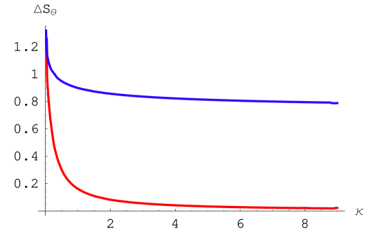
Figure 3: The boundary entropy $\Delta S_{\theta}=S_{\theta}-\log({\rm g}^{2}_{D})$ (51) for the circular brane model, as a function of the dimensionless inverse temperature $\kappa$ for $\theta=0,\pi$, derived from (14) and (26).

Omitting details, we would like to mention here that using methods developed in [21] (see also [13, 23]) one can reduce the calculation of the Wronskians (14), (26) at special values of the parameters to solution of certain system of nonlinear integral equations, the “TBA system”. For example, for integer $n$ and

$$P=0\,,\ \ \ \ \ Q=\pm{1\over\sqrt{n+2}}\,,$$ (53)

the amplitude $Z(\,{\bf P}\,|\,\kappa)$ (7) is expressed through solution of the $D_{n}$-type TBA system, associated with the diagram in Fig. 4. It is remarkable that this system coincides exactly with the system of TBA equations for the Toulose limit of the $n$-channel Kondo model [22], while the entropy $S^{\rm(Kondo)}_{j}$ of the impurity spin $j={n-1\over 2}$ is given by

$$S^{\rm(Kondo)}_{n-1\over 2}=\Big{(}\,1-\kappa\,{\mbox{d}\over{\mbox{d}\kappa}}\,\Big{)}\,\log\big{(}\,{\rm g}_{D}^{-4}\ Z_{\theta=0}(\,{\bf P}^{*}\,|\,\kappa\,)\ Z_{\theta=\pi}(\,{\bf P}^{*}\,|\,\kappa\,)\,\big{)}\ ,$$ (54)

where ${\bf P}^{*}=\big{(}0\,,\,{\textstyle{1\over\sqrt{n+2}}}\,\big{)}$ and $E_{*}$ is identified with the Kondo temperature. Notice that at this choice of $P,Q$ the coefficient $t_{1}$ in the low-temperature expansion of the partition function (30) vanishes and the expansion starts with $t_{2}$ (see Table 2 in Appendix). Also, this TBA system (see Fig. 4) differs only in the structure of the “source terms” from the TBA system associated with the $H_{n}^{(0)},\,H_{n}^{(\pi)}$ models [24], which are certain integrable perturbations of the minimal ${\mathbb{Z}}_{n}$-parafermionic CFT.

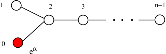
Figure 4: Incidence diagram for the TBA system in the case of the paperclip brane with an integer $n\geq 3$ and $P=0,\ Q=\pm{1\over\sqrt{n+2}}$. The source term indicated near the corresponding node.

At $n=\infty$, the boundary entropy of the circular brane model with $\theta=0,\,\pi$ is given by

$$\Delta S_{\theta=k\pi}(\kappa)=\int_{-\infty}^{\infty}{\mbox{d}\beta\over 2\pi}\ \mbox{e}^{\gamma-\beta}\ \ {\log\big{[}1+\mbox{e}^{-\varepsilon_{k}(\beta)}\big{]}\over\cosh^{2}(\beta-\gamma)}\,\ \ \ \ \ \ \ (k=0,\,1)\ ,$$ (55)

where $\gamma=\log(4\pi\kappa)$ and $\varepsilon_{k},\ k=0,1,2,\ldots$ solve the infinite chain of integral equations:

$$0 = \varepsilon_{k}(\alpha)+\int_{-\infty}^{\infty}{\mbox{d}\beta\over 2\pi}\ {\log\big{[}\big{(}1+\mbox{e}^{-\varepsilon_{k+1}(\beta)}\big{)}\,\big{(}1+\mbox{e}^{-\varepsilon_{k-1}(\beta)}\big{)}\big{]}\over\cosh(\beta-\alpha)}+$$ (56)

$$\delta_{k,2}\ \int_{-\infty}^{\infty}{\mbox{d}\beta\over 2\pi}\ {\log\big{[}1+\mbox{e}^{-\varepsilon_{0}(\beta)}\big{]}\over\cosh(\beta-\alpha)}\ \ \ \ (k=2,\,3,\,4\ldots\infty)\ ,$$

$$\mbox{e}^{\alpha}\ \delta_{k,0} = \varepsilon_{k}(\alpha)+\int_{-\infty}^{\infty}{\mbox{d}\beta\over 2\pi}\ {\log\big{[}1+\mbox{e}^{-\varepsilon_{2}(\beta)}\big{]}\over\cosh(\beta-\alpha)}\ \ \ \ (k=0,\,1)\ .$$

To sunmmarize, we have proposed exact partition function of a nontrivial model of boundary interaction – the paperclip model. There are parallels between this model on one side, and the bulk sigma-models such as the $O(3)$ nonlinear sigma model and the “sausage” model [7] on the other. In particular, according to our proposal, the addition of the topological term with $\theta=\pi$ in the paperclip model leads to a non-trivial IR fixed point. In the limit when the parameter $n$ goes to infinity the paperclip model reduces to the “circular brane”, which is equivalent to the Ambegaokar-Eckern-Schön model of a quantum dot. At finite integer $n$ our proposal suggests intriguing formal relation to the $n$-channel Kondo model in the Toulose limit.

Appendix

Here we present an integral representation for the second coefficient $t_{2}$ appeared in the expansion (30), which was obtained by an analytic technique developed in Appendix A of Ref.[18]. Bellow we use the following notations

$$\xi={1\over n+2}\ ,\ \ \ p=\sqrt{n}\ \ {P\over 2}\,,\ \ \ \ q=\sqrt{n+2}\ \ {Q\over 2}\ .$$ (57)

The coefficient $t_{2}$ can be written as

$$t_{2}=-4\,\sin^{2}(\pi\xi)\cos\big{(}2\pi\xi(q+1)\big{)}\,a^{2}_{1}-4\,\sin(2\pi\xi)\sin\big{(}2\pi(q+1)\xi\big{)}\,a_{2}\,.$$ (58)

Here

$$a_{1}=(2\xi)^{-2\xi}\,{\Gamma(\xi)\Gamma({1\over 2}-\xi)\over 2\,\sqrt{\pi}}\,\bigg{[}\,{1-2\xi\over 2(1+2\xi)}+{p^{2}\over 2\,(q^{2}-{1\over 4})}\,\bigg{]}\,{\Gamma(1+(2q+1)\xi)\over\Gamma((2q-1)\xi)},$$ (59)

and $a_{2}$ in (58) admits the following representation for ${\Re e}\,q>0$ and $0<\xi<{1\over 2}\ \big{(}\xi\not={1\over 4}\big{)}$:

$$a_{2}={\Gamma\big{(}1+2\xi(q+1)\big{)}\over\Gamma\big{(}2\xi(q-1)\big{)}}\ \Big{(}\,{A\over q^{2}-1}+B+C\,\Big{)}\ ,$$ (60)

where

$$A = -(2\xi)^{-4\xi}\ {\Gamma(1+2\xi)\,\Gamma({1\over 2}-2\xi)\over 8\xi\ \sqrt{\pi}}\ \Big{(}p^{2}+{1\over 4}\Big{)}^{2}+$$ (61)

$$(4\xi)^{-4\xi}\ {\sqrt{\pi}\Gamma({1\over 2}-2\xi)\Gamma^{2}(1+3\xi)\over 4\xi\,\Gamma^{2}({1\over 2}+\xi)\Gamma(1+2\xi)}\ \bigg{[}{1-2\xi\over 2(1+2\xi)}+{2p^{2}\over 3}\,\bigg{]}^{2}\ ,$$

$$B = (2\xi)^{-4\xi}\ {\Gamma(1+2\xi)\,\Gamma({5\over 2}-2\xi)\over 8\xi\,\sqrt{\pi}\,(1+4\xi)}\ ,$$

$$C = {(2\xi)^{-4\xi}\over 8\Gamma^{2}(1-\xi)\Gamma^{2}({1\over 2}+\xi)}\times$$

$$\int_{-\infty}^{\infty}{\mbox{d}\tau\over 2\pi}\,{F(\tau)\,\sinh(2\pi\tau)\over(\tau+\mbox{i}q\xi)(\tau-\mbox{i}\xi)(\tau+\mbox{i}\xi)}\,\bigg{[}\,{1-2\xi\over 2(1+2\xi)}-{2\xi^{2}\,p^{2}\over 4\tau^{2}+\xi^{2}}\,\bigg{]}^{2}\,,$$

with

$$F(\tau)=\Gamma(1-2\xi+2\mbox{i}\tau)\Gamma(1-2\xi-2\mbox{i}\tau)\Gamma^{2}(1+\xi+2\mbox{i}\tau)\Gamma^{2}(1+\xi-2\mbox{i}\tau)\ .$$

Notice that for $\xi={1\over 4}\ (n=2)$ one has to use the L’${\hat{\rm o}}$pital’s rule to evaluate $a_{2}$ from Eq. (60). Using (58) it is straightforward to study the large $n$-behavior $(\xi\to 0)$ of $t_{2}$:

$$t_{2}=2\pi^{2}\ \xi^{2}\ \big{[}\,\xi\,\mbox{e}^{2+\gamma_{E}}\,\big{]}^{-4\xi}\,\Big{[}\,1-2q^{2}-2p^{2}-(3-4q^{2}+4p^{2})\ \xi+$$ (62)

$$\Big{\{}\,4+{\textstyle{\pi^{2}\over 24}}-\pi^{2}\,\big{(}\,q^{2}-2\,q^{4}-{\textstyle{2\over 3}}\,p^{4}-\big{(}{\textstyle{8\over\pi^{2}}}-{\textstyle{1\over 3}}\big{)}\,p^{2}-{8\over 3}\,q^{2}\,p^{2}\,\big{)}\Big{\}}\,\xi^{2}+O(\xi^{3})\,\Big{]}\,.$$

The above representation is very useful in numerical evaluation of this coefficient because of the fast convergency of the integral in (61). In Table 2 we present the numerical values of the coefficient $t_{2}$ at some integer $n$ and $P,\ Q$ given by Eq. (53). These numbers were also confirmed by numerical integration of the TBA system depicted in Fig. 4.

$n$	$\quad t_{2}$
1	0
2	${\sqrt{2}\over 48}$
3	$0.0546105$
4	$0.0661040$
5	$0.0683646$
6	$0.0658731$
7	$0.0613178$
8	$0.0561029$
9	$0.0509101$
10	$0.0460445$

Table 2: Numerical values of the second coefficient $t_{2}$ in the expansion (30) for $P=0,\ Q=\pm{1\over\sqrt{n+2}}$.

References

- [1] S.L. Lukyanov, E.S. Vitchev and A.B. Zamolodchikov, Nucl. Phys. B683, 423 (2004).
- [2] S.L. Lukyanov and A.B. Zamolodchikov, J. Stat. Mech.: Theor. Exp. P05003 (2004) (stacks.iop.org/JSTAT/2004/P05003).
- [3] V. Ambegaokar, U. Eckern and G. Schön, Phys. Rev. Lett. 48, 1745 (1982).
- [4] K.A. Matveev, Phys. Rev. B51, 1743 (1995).
- [5] A. Furusaki and K.A. Matveev, Phys. Rev. B51, 16878 (1995).
- [6] I.L. Aleiner, P.W. Brower and L.I. Glazman, Phys. Rep. 358, 309 (2002).
- [7] V.A. Fateev, E. Onofri and Al.B. Zamolodchikov, Nucl. Phys. B406, 521 (1993).
- [8] F.D.M. Haldane, J. Appl. Phys. 57, 3359 (1985).
- [9] I. Affleck, Field theory methods and quantum critical phenomena, in: Fields, strings and critical phenomena, eds. E. Brzin and J. Zinn-Justin (North-Holland, Amsterdam, 1990).
- [10] A.B. Zamolodchikov and Al.B. Zamolodchikov, JETP Lett. 26, 457 (1977); Nucl. Phys. B133, 525 (1978).
- [11] A.B. Zamolodchikov and Al.B. Zamolodchikov, Nucl. Phys. B379, 602 (1992).
- [12] P. Dorey and R. Tateo, J. Phys. A32, L419 (1999).
- [13] V.V. Bazhanov, S.L. Lukyanov and A.B. Zamolodchikov, Jour. Stat. Phys. 102, 567 (2001).
- [14] V.V. Bazhanov, A.N. Hibberd and S.M. Khoroshkin, Nucl. Phys. B622, 475 (2002).
- [15] V.V. Bazhanov, S.L. Lukyanov and A.M. Tsvelik, Phys. Rev. B68, 094427 (2003).
- [16] I. Affleck and A. Ludwig, Phys. Rev. Lett. 67, 161 (1991).
- [17] L.D. Landau and E.M. Lifshitz, Quantum Mechanics: Non-Relativistic Theory, Vol.3, Third Edition Pergamon Press, Oxford (1997).
- [18] V.V. Bazhanov, S.L. Lukyanov and A.B. Zamolodchikov, Nucl. Phys. B549, 529 (1999).
- [19] A.H. Castro Neto, E. Novais, L. Borda, G. Zarand and I. Affleck, Phys. Rev. Lett. 91 206403 (2003).
- [20] D. Friedan and A. Konechny, Phys. Rev. Lett. 93, 030402 (2004).
- [21] A. Voros, J. Phys. A32, 5993 (1999).
- [22] A.M. Tsvelik, Phys. Rev. B52, 4366 (1995).
- [23] P. Dorey and R. Tateo, Nucl. Phys. B563, 573 (1999).
- [24] V.A. Fateev and Al.B. Zamolodchikov, Phys. Lett. B271, 91 (1991).