Abstract: We present non-perturbative results for $U(1)$ gauge theory in spaces, which include a non-commutative plane. In contrast to the commutative space, such gauge theories involve a Yang-Mills term, and the Wilson loop is complex on the non-perturbative level. We first consider the 2d case: small Wilson loops follows an area law, whereas for large Wilson loops the complex phase rises linearly with the area. In four dimensions the behavior is qualitatively similar for loops in the non-commutative plane, whereas the loops in other planes follow closely the commutative pattern. In $d=2$ our results can be extrapolated safely to the continuum limit, and in $d=4$ we report on recent progress towards this goal.

1 Non-commutative $U(1)$ gauge theory

We consider the simplest version of non-commutative (NC) spaces: only two (Euclidean) coordinates are NC, and the non-commutativity parameter $\theta$ is constant,

$$[\hat{x}_{i},\hat{x}_{j}]=i\,\theta\,\epsilon_{ij}\qquad({\rm indices}~{}~{}i,j\in\{1,2\})\ .$$ (1)

According to a historic observation by Peierls [2], such coordinates describe a charged particle moving in a (commutative) plane, which is crossed by a strong, orthogonal magnetic field $B$. In fact, if we ignore the kinetic term in the Lagrangian, such a particle has the canonical momentum $p_{i}=qB\epsilon_{ij}x_{j}$, where $q$ is the electric charge. Under canonical quantization we obtain

$$[\hat{x}_{i},\hat{p}_{i}]=i\hbar=qB\epsilon_{ij}[\hat{x}_{i},\hat{x}_{j}]\ ,$$ (2)

which is a NC relation with $\theta\propto 1/B$. Based on this idea, NC field theory plays a rôle as a formalism in solid state physics.

A similar idea is also used to map string theory in a magnetic background onto NC field theory. The construction of this mapping [3] has tremendously boosted the interest in NC field theories (i.e. field theories on NC spaces).

An important mathematical result states that we can return to the use of ordinary (commutative) coordinates if all the fields are multiplied by star products,

$$\phi(x)\star\psi(x):=\phi(x)\exp\Big{(}\,\frac{1}{2}\mathop{\raise 7.23328pt\hbox{$\leftarrow$\kern-9.00002pt\raise-7.23328pt\hbox{$\partial$}}}\,\!_{i}\,\theta\,\epsilon_{ij}\,\vec{\partial}_{j}\,\Big{)}\ \psi(x)\ .$$ (3)

Here we focus on pure $U(1)$ gauge theory, which has the Euclidean action

$$S[A] = \frac{1}{4}\int d^{4}x\,F_{\mu\nu}\star F_{\mu\nu}\ ,$$

$$F_{\mu\nu} = \partial_{\mu}A_{\nu}-\partial_{\nu}A_{\mu}+ig[A_{\mu},A_{\nu}]_{\star}\ ,$$ (4)

where the last term is a star-commutator. This action is star-gauge invariant, i.e. invariant under transformations

$$A_{\mu}(x)\to U(x)\star A_{\mu}(x)\star U(x)^{\dagger}-\frac{i}{g}U(x)\star\partial_{\mu}U(x)^{\dagger}\ ,$$ (5)

where $U(x)$ is star-unitary, $U(x)^{\dagger}\star U(x)=1\!\!1$.

Other $U(N)$ gauge theories may be studied along the same lines, but the formulation of $SU(N)$ gauge theories runs into trouble on NC spaces. To see this problem, let us represent the gauge field as $A_{\mu}^{a}T_{a}$, $T_{a}$ being the Hermitian generators of the gauge group. Then the star commutator can be decomposed as

$$2\ [A_{\mu}^{a}T_{a},A_{\nu}^{b}T_{b}]_{\star}=[A_{\mu}^{a},A_{\nu}^{b}]_{\star}\cdot\{T_{a},T_{b}\}+\{A_{\mu}^{a},A_{\nu}^{b}\}_{\star}\cdot[T_{a},T_{b}]\ .$$ (6)

If we deal with $SU(N)$ gauge theory we have the additional condition ${\rm Tr}\,T_{a}=0$, which should be reproduced by the star-commutator for the algebra to close. In the commutative case, $\theta=0$, the first term vanishes ( $[A_{\mu}^{a},A_{\nu}^{b}]=0$ ). Then the algebra closes because ${\rm Tr}\,[T_{a},T_{b}]$ trivially vanishes. For finite $\theta$, however, also the first term contributes, which causes trouble (because ${\rm Tr}\,\{T_{a},T_{b}\}\propto\delta_{ab}$ does not vanish).

Therefore it is motivated to concentrate on $U(1)$ as a physical gauge group, which can be accommodated on a NC space.

2 Mapping onto a twisted Eguchi-Kawai model

As a first step towards a formulation to be used in Monte Carlo simulations, we introduce a lattice structure in the NC plane. Since all space-points are somewhat fuzzy, we cannot expect sharp lattice sites, but the operator identity

$$\exp\Big{(}i\frac{2\pi}{a}\hat{x}_{i}\Big{)}=\hat{1}\!\!1$$ (7)

does nevertheless impose a lattice structure with lattice spacing $a$. If we require the momentum components $k_{i}$ to be periodic over the Brillouin zone, the above condition implies that only discrete momenta occur (see e.g. [4]), which is characteristic for a finite volume. If we assume a periodic $N\times N$ lattice, the allowed momenta are separated by  $\Delta k_{i}=\frac{2\pi}{aN}$,  and the non-commutativity parameter can be identified as

$$\theta=\frac{1}{\pi}Na^{2}\ .$$ (8)

Therefore we are interested in a double scaling limit $a\to 0$, $N\to\infty$ with $Na^{2}=const.$, which leads to a continuous non-commutative plane of infinite extent.

However, even on the lattice it is far from obvious how to simulate NC gauge theory; note that this seems to require star-unitary link variables. It is highly profitable to map the system (or its NC part) onto a twisted Eguchi-Kawai model. The latter is defined on a single space-point and its action has the form [5]

$$S_{\rm TEK}[U]=-N\beta\sum_{i\neq j}Z_{ij}{\rm Tr}\,\Big{(}U_{i}U_{j}U_{i}^{\dagger}U_{j}^{\dagger}\Big{)}\ .$$ (9)

$U_{1}$ and $U_{2}$ are unitary $N\times N$ matrices which encode the degrees of freedom of the lattice model, and the twist factor is chosen here as $Z_{21}=Z_{12}^{*}=\exp(\pi i(N+1)/N)$, where $N$ has to be odd. Then there is an exact equivalence to the lattice NC gauge theory, i.e. the algebras are fully identical, as Ref. [6] showed in the large $N$ limit. A refined consideration found such a mapping even at finite $N$ [7]. This is the form which is suitable for numerical simulations.

It is straightforward to formulate (the analogue of) Wilson loops in the framework of the matrix model,

$$W_{ij}(I\times J)=\frac{1}{N}Z_{ij}^{\pm IJ}\ {\rm Tr}\,\Big{(}U_{i}^{I}U_{j}^{J}U_{i}^{\dagger\,I}U_{j}^{\dagger\,J}\Big{)}\ .$$ (10)

This corresponds to a rectangular Wilson loop of sides $aI$ and $aJ$. Mapping this quantity back to the lattice leads in fact to a sensible definition of a Wilson loop in the NC gauge theory [8]. The exponent of the twist factor is taken positive (negative) for an anti-clockwise (clockwise) orientation. The Wilson loop is complex in general, although this property cannot be seen perturbatively in $d=2$ [9]. For further perturbative studies we refer to Refs. [10], and to Refs. [11] for semi-classical approaches.

3 Numerical results

3.1 Two dimensions

In the planar limit of the two dimensional model we obtain the commutative $U(N\to\infty)$ lattice gauge theory on a plane, which was solved by Gross and Witten by studying Wilson loops [12]. In this limit they found an exact area law. We tested that the values of $N$, which are accessible to our simulations, do approximate the planar limit well by checking the validity of the large $N$ Schwinger-Dyson equations, along with the large $N$ factorization. On the lattice, they relate Wilson loops of different shapes in the planar limit. An example for the corresponding contours is illustrated in Figure 1. This was the property that the original work by Eguchi and Kawai (without twist) was based on [13]. Indeed, we observe that our measurements for the two sides of such equations converge as we increase $N$ to a magnitude of a few hundred, keeping $\beta$ fixed, for instance at $0.25$. This is shown in Figure 2, see also Ref. [14].

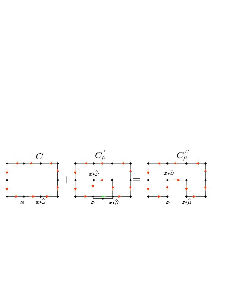
Figure 1: An example for a set of contours, which are involved in a Schwinger-Dyson equation. These equations relate the corresponding Wilson loops in the planar limit.

Figure 2: The convergence towards the validity of the Schwinger-Dyson equations as $N$ increases at fixed $\beta=0.25$. On the $x$-axis of the plot on the left we show the area of the contour called $C$ in Figure 1. On the right we show the convergence in $N$ at a fixed area of $7\times 8$ for the contour $C$. Note that in a common normalization — with a prefactor $1/N$ for the Wilson loops — our result is consistent with the expected finite $N$ artifacts of the order of $1/N^{2}$.

Hence we can use this limit to identify the lattice spacing as $\beta\propto 1/a^{2}$, as in the result by Gross and Witten. Therefore we take the double scaling limit by keeping the ratio $N/\beta$ constant.

In Figure 3 we show our simulation results [15] for the Wilson loop

$$W(I)=\langle W_{12}(I\times I)\rangle$$ (11)

in polar coordinates, as a function of the physical (i.e. dimensionful) area $(aI)^{2}$. We choose $N$ over a broad range, with a fixed ratio $N/\beta=32$.

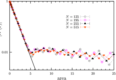
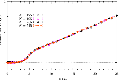
Figure 3: We show square shaped Wilson loops $W(I)$ on a NC plane: from the plot on the left we see that small loops follow the Gross-Witten area law (which is marked by a line). At large areas the absolute value does not decay any further, but a linearly rising phase sets in, as the plot on the right shows.

From Figure 3 we infer the following properties:

• The observable $W(I)$ does indeed stabilize in the double scaling limit. Thus we have found a new universality class. In particular this shows that the model is non-perturbatively renormalizable.

• At small area, the absolute value follows the Gross-Witten area law, which is marked by a line in the plot on the left-hand-side of Figure 3. In that regime the phase is practically zero, hence Wilson loops with areas $A=(aI)^{2}\mathop{\raise 1.55pt\hbox{$<$\kern-9.00002pt\raise-5.68335pt\hbox{$\sim$}}}4$ follow the behavior the behavior of commutative large $N$ gauge theory.

• For larger areas, the absolute value does not decay any further, but the phase starts to increase linearly in the area.

Regarding the second point — the area law for small Wilson loops — we also measured the Creutz ratio,

$$\chi(I,J)=-\log\Big{(}\frac{W(I\times J)W((I-1)\times(J-1))}{W((I-1)\times J)W(I\times(J-1))}\Big{)}\ ,$$ (12)

which singles out the string tension $\sigma$ for decays $\propto\exp(-\sigma A)$. Typical results for (nearly) square shaped Wilson loops, $\chi(I,I)$, as well as extremely anisotropic (rectangular) Wilson loops, $\chi(2,J)$, are shown in Figure 4 on the left. We see a stable value $\sigma\approx 1$ as long as we are well inside the area law regime, and a marked deviation from it as the area approaches its critical value.

In view of the third observation — the linearly rising phase — we performed further tests with different ratios $N/\beta=16,\ 24,\ 48$, i.e. different values of $\theta$, see Figure 4 on the right, and also with rectangular loops. At large areas we always found to a very high precision the simple relation

$${\rm Phase}=\frac{A}{\theta}=A\cdot B\ .$$ (13)

In the last term we introduced a formal magnetic field $B=1/\theta$, in the spirit of Peierls’ map.

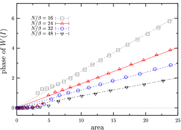
Figure 4: On the left: the Creutz ratio for Wilson loops with small areas, up to the transition observed in Figure 3. On the right: the linearly increasing phase at various values of the non-commutativity parameter $\theta$, in agreement with eq. (13).

This behavior corresponds exactly to the Aharonov-Bohm effect. It is known from the corresponding magnetic fields in string theory and in solid state physics, where it is implemented on tree level. Here, however, we recover the very same behavior unexpectedly as a dynamical effect at low energy.

One may wonder why the short-ranged non-commutativity has striking effects on the large rather than the small Wilson loops. Apparently there is some UV/IR mixing [16] going on, even though there are no divergences in the perturbative expansion of this model. This suggests that UV/IR mixing occurs non-perturbatively, and it belongs therefore to the fundamental nature of NC field theory. This is in agreement with analytic [17] and numerical [18] results for the NC $\lambda\phi^{4}$ model.

3.2 Four dimensions

We now proceed to four dimensions, which include a NC plane, as well as two commutative coordinates — among them is the Euclidean time. Therefore we deal with one NC plane, one commutative plane and 4 mixed planes, and we will distinguish the (flat) Wilson loops accordingly.

There are 1-loop studies about the photon dispersion relation in such spaces [19]. Computations of the $\beta$ function indicate asymptotic freedom [20]. Other perturbative studies suggest that this model may have a negative IR divergence, which would render it unstable and unsuitable to describe physics [21]. More precisely, those works suggest that bosonic (fermionic) degrees of freedom contribute negative (positive) IR poles, and they therefore proceed to SUSY models. Here we stay in the simple bosonic framework; of course we would like to verify this claim on a non-perturbative level.

Again we introduce a lattice formulation and map the NC plane on a twisted Eguchi-Kawai model; one on each lattice point of the remaining (commutative) plane. On the technical side, it is very important to apply the heat bath algorithm for the simulations. This is not straightforward, since this matrix model is non-linear in the link variables. For our 2d model a method to linearize it with the help of auxiliary fields was introduced by Fabricius and Haan [22]. We also applied it in our simulations, which led to the results in the previous Subsection. In $d=4$ it turned out that this method is still applicable in a generalized form [23], which allows us to use the powerful heat bath algorithm. Without it, it is very hard to overcome the problems related to thermalization and autocorrelation [24].

We first present simulation results at $N=25$ [25]. The left side of Figure 5 shows the real part of the plaquette values at different $\beta$. In this case all six possible orientations of the plaquettes are averaged over. The results match the anticipated asymptotic behavior [5] of the plaquette expectation value $\langle P\rangle$: at weak coupling is behaves as $\sim 1-\frac{1}{8\beta}$ and at strong coupling as $\sim\beta$. A phase transition occurs around $\beta\approx 0.35$. All the results that we show in the following were obtained in the weak coupling phase.

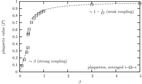
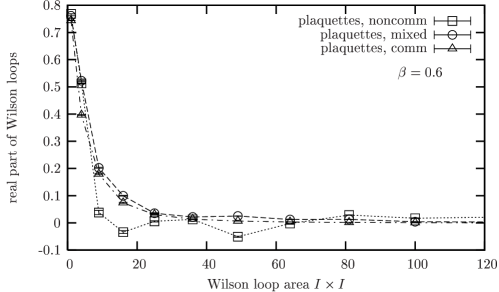
Figure 5: On the left: The real part of the plaquettes, averaged over all possible orientations. The dashed lines show the asymptotic behavior expected from expansion in strong resp. weak coupling. On the right: The real part of the plaquettes, plotted separately according to their orientation.

The decay of square shaped Wilson loops with increasing area is shown in Figure 5 on the right. In that plot the results are separated according to the plaquette orientations (NC, mixed and commutative). The real part of the NC Wilson loops performs a damped oscillation around zero. This is in qualitative agreement with the observations in $d=2$. For the other two types of Wilson loops the real part decays monotonously towards zero.

We have again measured the Creutz ratios for various rectangular Wilson loops [25]. The (dimensionless) string tension approaches zero as $\beta\rightarrow\infty$.

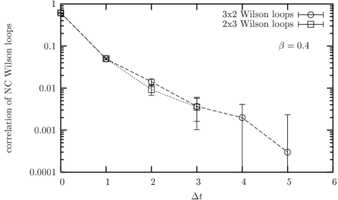
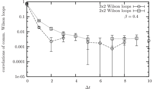
Figure 6: Temporal correlation of the plaquettes lying completely in the NC plane (on the left) and completely in the commutative plane (on the right). In the former case only we see a trend towards an exponential decay.

Figure 6 (on the left) shows the correlation function of the plaquettes lying completely in the NC plane, separated by $\Delta t$ in Euclidean time. These data were taken at $\beta=0.4$, i.e. barely in the weak coupling phase. The decay is likely to be exponential, but a higher statistics is required to verify this behavior.

The analogous plot for plaquettes in the commutative plane is shown in Figure 6 on the right. In that case the decay does not seem exponential.

At last, we illustrate our progress in the search for a double scaling limit. In contrast to $d=2$, we do not have an analytic result in the planar limit to identify the physical lattice spacing (i.e. to relate $\beta$ and $a$). However, we observed that double scaling is approximated quite well if we assume ad hoc the simple relation $\beta\propto 1/a$, so that the double scaling limit keeps $N/\beta^{2}=const.$ In particular we set this ratio to $20$ and obtained the results for the real parts of square shaped Wilson loops shown in Figure 7. We are also working on a systematic search for double scaling by matching the data without any assumption about the relation between $\beta$ and $a$. This represents a completely unbiased test of the result presented here.

Figure 7: We show the real part of Wilson loops in the three types of planes (commutative, mixed and NC) of our 4d space. Here we have fixed $N/\beta^{2}=20$. The results approximate a double scaling behavior decently well. (We always refer to $N\times N$ matrices for the NC plane, and a $(N-1)\times(N-1)$ lattice on the commutative plane.)

4 Conclusions

We have simulated NC $U(1)$ field theory in $d=2$ and in $d=4$. In $d=2$ we observed an area law for Wilson loops with small area, as expected from the equivalence to commutative large $N$ gauge theory in the UV regime. At large area, a phase starts to increase linearly in the area, which is reminiscent of the Aharonov Bohm effect.

The simulations in $d=4$ (with two NC coordinates) are still on-going. We first measured the action, plaquettes, Wilson loops and Creutz ratios. The results for the action and plaquettes agree with asymptotic predictions. There seems to be a vanishing string tension at weak coupling in the part of the parameter space we explored. The Wilson loops in the NC plane show a behavior similar to the 2d NC model, whereas the loops in other planes are close to the commutative feature.

We found a simple ad hoc ansatz which seems to provide quite well a double scaling limit. This ansatz is still being checked with a fully systematic approach. The double scaling limit corresponds to the model at zero lattice spacing and in infinite volume, hence its identification is a milestone in the non-perturbative analysis of this model. Thus we hope to glimpse at the dispersion relations for the NC photon, which might allow us to confront the theory with phenomenological data.

Even before that, however, it is important to clarify if this model is actually IR stable.

Acknowledgement It is a pleasure to thank Jan Ambjørn, Aiyalam Balachandran, Simon Catterall, Harald Dorn, Giorgio Immirzi, Esperanza Lopez, Yuri Makeenko, Denjoe O’Connor, Richard Szabo and Alessandro Torrielli for stimulating discussions. We are also grateful to the “Deutsche Forschungsgemeinschaft” (DFG) for generous support. An important part of the computations were performed on the IBM p690 clusters of the “Norddeutscher Verbund für Hoch- und Höchstleistungsrechnen” (HLRN). Finally we thank Hinnerk Stüben for his advice on the parallelization of our codes.

References

- [1]
- [2] R. Peierls, Z. Phys. 80 (1933) 763.
- [3] N. Seiberg and E. Witten, JHEP 09 (1999) 032.
- [4] R.J. Szabo, Phys. Rep. 378 (2003) 207.
- [5] A. González-Arroyo and M. Okawa, Phys. Rev. 27D (1983) 2397.
- [6] H. Aoki, N. Ishibashi, S. Iso, H. Kawai, Y. Kitazawa and T. Tada, Nucl. Phys. B565 (2000) 176.
- [7] J. Ambjørn, Y.M. Makeenko, J. Nishimura and R.J. Szabo, JHEP 11 (1999) 29; Phys. Lett. B480 (2000) 399; JHEP 05 (2000) 023.
- [8] N. Ishibashi, S. Iso, H. Kawai and Y. Kitazawa, Nucl. Phys. B573 (2000) 573.
- [9] J. Ambjørn, A. Dubin and Y. Makeenko, JHEP 0407 (2004) 044.
- [10] A. Bassetto, G. Nardelli and A. Torrielli, Nucl. Phys. B617 (2001) 308; Phys. Rev. D66 (2002) 085012. A. Bassetto, G. De Pol and F. Vian, JHEP 0306 (2003) 051.
- [11] L. Griguolo, D. Seminara and P. Valtancoli, JHEP 0112 (2001) 024. L.D. Paniak and R.J. Szabo, Commun. Math. Phys. 243 (2003) 343; JHEP 0305 (2003) 029. A. Bassetto and F. Vian, JHEP 0210 (2002) 004. H. Dorn and A. Torrielli, JHEP 0401 (2004) 026.
- [12] D.J. Gross and E. Witten, Phys. Rev. D21 (1980) 446.
- [13] T. Eguchi and H. Kawai, Phys. Rev. Lett. 48 (1982) 1063.
- [14] T. Nakajima and J. Nishimura, Nucl. Phys. B528 (1998) 355.
- [15] W. Bietenholz, F. Hofheinz and J. Nishimura, JHEP 09 (2002) 9.
- [16] S. Minwalla, M. van Raamsdonk and N. Seiberg, JHEP 02 (2000) 020.
- [17] S.S. Gubser and S.L. Sondhi, Nucl. Phys. B605 (2001) 395. G.-H. Chen and Y.-S. Wu, Nucl. Phys. B622 (2002) 189. P. Castorina and D. Zappalà, Phys. Rev. D68 (2003) 065008. W. Bietenholz, F. Hofheinz and J. Nishimura, JHEP 0405 (2004) 047.
- [18] W. Bietenholz, F. Hofheinz and J. Nishimura, Nucl. Phys. (Proc. Suppl.) 119 (2003) 941; Fortsch. Phys. 51 (2003) 745; Acta Phys. Polonica B34 (2003) 4711; JHEP 06 (2004) 42. J. Ambjørn and S. Catterall, Phys. Lett. B549 (2002) 253.
- [19] M. Hayakawa, hep-th/9912167. A. Matusis, L. Susskind and N. Toumbas, JHEP 12 (2000) 2. F. Ruiz Ruiz, Phys. Lett. B502 (2001) 274.
- [20] C.P. Martin and D. Sánchez-Ruiz, Phys. Rev. Lett. 83 (1999) 476. T. Krajewski and R. Wulkenhaar, Int. J. Mod. Phys. A15 (2000) 1011.
- [21] M. van Raamsdonk, JHEP 0111 (2001) 006. K. Landsteiner, E. Lopez and M.H. Tytgat, JHEP 0106 (2001) 055. A. Armoni and E. Lopez, Nucl. Phys. B632 (2002) 240. Z. Guralnik, R.C. Helling, K. Landsteiner and E. Lopez, JHEP 0205 (2002) 025.
- [22] K. Fabricius and O. Haan, Phys. Lett. 143B (1984) 459.
- [23] Y. Susaki, private notes.
- [24] S. Profumo and E. Vicari, JHEP 0205 (2002) 014.
- [25] W. Bietenholz, F. Hofheinz, J. Nishimura, Y. Susaki and J. Volkholz, hep-lat/0409059.