Multiple Inflation, Cosmic String Networks and the String Landscape

Abstract:

Motivated by the string landscape we examine scenarios for which inflation is a two-step process, with a comparatively short inflationary epoch near the string scale and a longer period at a much lower energy (like the TeV scale). We quantify the number of $e$-foldings of inflation which are required to yield successful inflation within this picture. The constraints are very sensitive to the equation of state during the epoch between the two inflationary periods, as the extra-horizon modes can come back inside the horizon and become reprocessed. We find that the number of $e$-foldings during the first inflationary epoch can be as small as 12, but only if the inter-inflationary period is dominated by a network of cosmic strings (such as might be produced if the initial inflationary period is due to the brane-antibrane mechanism). In this case a further 20 $e$-foldings of inflation would be required at lower energies to solve the late universe’s flatness and horizon problems.

1 Introduction and Summary

The search for inflationary solutions within string theory is still young, but considerable progress has been made over the past several years. Most of this recent progress began with the recognition that the separation of two branes could function as an inflaton [1], and that configurations of branes and antibranes together break supersymmetry in a calculable way, potentially allowing the explicit computation of the resulting inflaton dynamics[2, 3, 4, 5, 6, 7]. Direct contact with string theory also became possible [9] with the recognition that moduli stabilization can be achieved at the string scale within a controllable approximation [10, 11].

Despite it still being a young topic, it is possible to draw some preliminary conclusions about the implications of embedding inflationary cosmology into string theory. In particular, the following two features are seen in a large set of models [12].

• It is no easier to obtain 60 $e$-foldings of inflation within string theory than in other models. For all of the known examples of inflation within string theory there are parameters and/or initial conditions which must be carefully tuned. The problem arises because inflation typically occurs at energies near the string scale, and so there are no particularly small dimensionless numbers from which to obtain inflation. Of course, the fewer $e$-foldings which are demanded, the less precise are the adjustments that are required.

• Although the most recent progress has focused on Type IIB vacua having few moduli, supersymmetric string vacua are usually littered with moduli, which generically acquire masses only after supersymmetry breaks. Thus we generically find numerous scalar fields whose masses are comparatively small, since they are close to the weak scale, $M_{w}$. Scalars of this type are usually anathema for cosmology since they cause a host of problems for cosmology [13] during the Hot Big Bang.

It has been suggested that these two problems may be each other’s solutions [12, 14]. For instance, suppose many fewer than 60 $e$-foldings of inflation occur up at the string scale, whose quantum fluctuations generate the large-scale structure which is presently visible as temperature fluctuations in the Cosmic Microwave Background (CMB). In this case the remaining $e$-foldings of inflation required by the horizon and flatness problems might plausibly be obtained during later epochs, when the many moduli are rolling around in the complicated potential landscape which is generated by low-energy supersymmetry breaking. This later period of inflation might be due to a mechanism which depends on the more complicated potentials expected in a low-energy theory involving very many would-be moduli, perhaps along the lines proposed in ref. [15, 16]. Besides solving the horizon and flatness problems, if it occurs at the weak scale this second stage of inflation could also solve some of the problems associated with moduli along the lines suggested in ref. [17].

Thus, it may be that a more generic picture of inflation within string theory is a two-step (or multi-step) process — as in Fig. 1 — given what we know about the low-energy potential landscape. If so, then there would be several observational consequences.

1. The observed CMB temperature fluctuations should not be deep within the slow-roll regime, since $N_{e}<60$ implies the slow roll parameters are likely to be larger: $\eta\sim 1/N_{e}>0.02$. In particular perhaps the slow-roll parameters might instead be of order $1/N_{e}\sim 0.1$ or larger. If so, then phenomena like kinks in the inflationary spectrum or a running spectral index would be much more likely to arise at observable levels. This realizes the folded inflation scenario [14], albeit with a long hiatus between inflation in the different directions in the landscape. This model is naturally compatible with a sizable tensor contribution to the observed spectrum of CMB anisotropies.

2. A period of late inflation would require the explanation of any post-inflationary processes like baryogenesis to take place at energies as low as the electroweak scale, with all of the associated observational implications which this would imply.

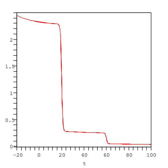
Figure 1: A sketch of the Hubble scale, $H$, during a two-step inflationary process. We imagine the first step to involve a minimal number of $e$-foldings at the string scale, followed by more $e$-foldings at the electroweak scale.

This paper examines the consequences of this kind of two-step inflationary cosmology. Our goal is to determine the minimal amount of inflation needed at high energies to produce the CMB temperature fluctuations, and how this minimal amount depends on the subsequent history of the universe. We employ general arguments based on energy conservation, and construct explicit toy models for inflationary potentials which exhibit multiple inflationary periods.

We note in passing that while the kind of two-stage inflation envisioned here may well involve less fine-tuning than a single, longer stage of inflation at higher energies. However, very unusual inflationary trajectories may still be “preferred” if they lead to vast amounts of inflation, as the low probability of such a hypothetical trajectory may be offset by the vast volume of space it produces [19].

The remainder of the paper is organized as follows. §2, which follows immediately, describes the bounds on the amounts of inflation which can be derived using only general arguments about the size and equation of state of the universe. This is followed, in §3, by a description of a toy field theory which has been designed to produce a simple concrete example having multiple inflationary epochs. In an appendix we present the most general set-up of multiple inflation and the total number of $e$-foldings required to solve the horizon problem. Our conclusions are summarized in §4.

2 General Constraints

Here we determine some general constraints on the number of $e$-foldings need in any two-step inflationary model. Our analysis follows closely that of ref. [20]. The essential features of the inflationary process we assume are captured by Fig. 1. This figure shows the Hubble scale over two inflationary epochs, followed by power-law evolution for the scale factor.

The constraints quantified in this section are of three types. First, we must ask for the total amount of expansion to be large enough to solve the horizon and flatness problems in the way which motivated inflationary scenarios in the first place. Second, we demand that the first inflationary phase lasts long enough to generate all of the primordial fluctuations which are observed on long scales during the present epoch. Finally, we require that none of the modes leaving the horizon during the first epoch of inflation are reprocessed in an observable way during the subsequent evolution of the universe.

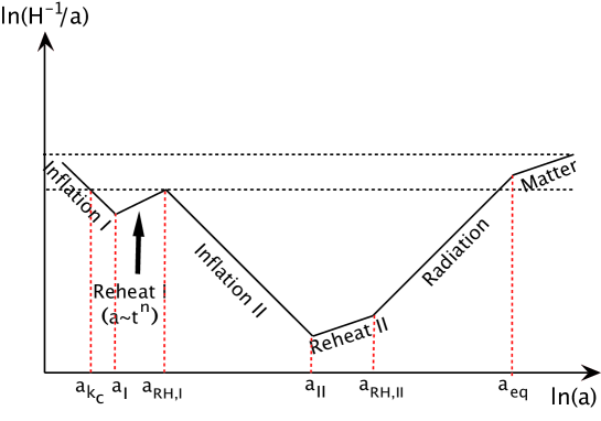
Figure 2: A sketch of the comoving Hubble scale during a two-step inflationary process. We plotted $\ln(H^{-1}/a)$ versus $\ln(a)$. During inflation by definition the comoving Hubble length decreases, otherwise it increases as it is shown in the figure. We parameterized the phase between the two inflationary epochs by a generic power law behavior with $n\leq 1$. For $n=2/3$ the Universe will be dominated by the matter dominated epoch, for $n=1/2$ the Universe is filled with radiation and for $n=1$ the expansion is dominated by the network of strings.

2.1 Cosmological Kinematics

In order to derive the constraints implied by these conditions, it is convenient to plot the quantity $\ell=1/(aH)$ against $a$, where $a$ is the scale factor and $H=da/dt$, as in Fig. 2. Inflationary epochs appear on such a plot as regions for which $\ell$ shrinks as $a$ increases, while for ordinary matter- or radiation-dominated epochs $\ell$ is a growing function of $a$. Since scales leave the horizon when their co-moving wave-number, $k$, satisfies $k/a=H$, the epochs when a particular mode is inside (or outside) of the horizon corresponds to the times when the curve for $y=\ell$ falls below (or above) a horizontal line drawn at $y=1/k$. For instance, the uppermost of the horizontal dotted lines in Fig. 2 corresponds to the scale, $k_{0}$, which is just re-entering the horizon at the present epoch.

As the picture makes clear, the last modes to leave the horizon during the first epoch of inflation subsequently re-enter the horizon during the interval before the second inflationary period. The lower line in Fig. 2 represents the critical scale, $k_{c}$, which is the last scale to re-enter in this way before the second inflationary epoch. The standard inflationary calculations for the density fluctuations produced by a mode assume that it does not get reprocessed in this way by the intermediate evolution between its initial horizon exit and its re-entry inside the horizon during the present epoch, and so in what follows we simplify the problem by demanding that none of the modes which are currently observable get reprocessed in this way.

Our goal is to quantify the conditions which must be satisfied by the number of $e$-foldings, $N_{I}$ and $N_{II}$, which occur during the two inflationary periods, defined as follows:

$$\textrm{e}^{N_{I}(k)}\equiv{a_{I}\over a_{k}},\ \qquad\textrm{e}^{N_{II}}\equiv{a_{II}\over a_{RH,I}}\,.$$ (1)

Here $a_{I}$ (and $a_{II}$) is the value of the scale factor at the end of first (and second) phase of inflation, while $a_{RH,I}$ similarly denotes the scale factor at the end of the ‘reheating’ period which occurs in between the two bouts of inflation.

Of particular interest is how short it is possible to make the initial inflationary period, $N_{I}$. For this reason it is also convenient to define the number, $\widetilde{N}$, of $e$-foldings of expansion between the time the critical scale $k_{c}$ leaves the horizon until the end of first inflationary period:

$$\textrm{e}^{\widetilde{N}}\equiv{a_{I}\over a_{k_{c}}}\,.$$ (2)

Since $N_{I}>\widetilde{N}$, it is important to know how large $\widetilde{N}$ must be, for various choices for the intermediate inflationary physics.

Following [20], we may derive a relationship amongst the quantities $N_{I}$, $N_{II}$ and $\widetilde{N}$, by expressing the condition that a particular mode, $k$, which enters the horizon at late times also left the horizon during the first inflationary epoch. That is, if a mode, $k$, leaves the horizon when the scale factor and Hubble scale had values $a_{k}$ and $H_{k}$, then the defining condition $k=a_{k}H_{k}$ implies:

$${k\over a_{0}H_{0}} = {a_{k}H_{k}\over a_{0}H_{0}}$$ (3)

$$= \left({a_{k}\over a_{I}}\right)\left({a_{I}\over a_{RH,I}}\right)\left({a_{RH,I}\over a_{II}}\right)\left({a_{II}\over a_{RH,II}}\right)\left({a_{RH,II}\over a_{eq}}\right)\left({H_{k}\over H_{eq}}\right)\left({a_{eq}H_{eq}\over a_{0}H_{0}}\right)$$

$$= \textrm{e}^{-N_{I}(k)}\left({a_{I}\over a_{RH,I}}\right)\textrm{e}^{-N_{II}}\left({a_{II}\over a_{RH,II}}\right)\left({\rho_{RH,II}\over\rho_{eq}}\right)^{-1/4}\left({H_{k}\over H_{eq}}\right)\left({a_{eq}H_{eq}\over a_{0}H_{0}}\right).$$

To obtain the final line above, we used the fact that $\rho_{r}\propto a^{-4}$ to replace ${a_{RH,II}\over a_{eq}}$, along with the Hubble scale at the present time, $H_{0}$, and at radiation-matter equality, $H_{eq}$. In what follows we take $H_{0}=h\,(100\,\hbox{km/s/Mpc})=1.75\times 10^{-61}\,h\,M_{p}$, where $h\approx 0.7$ and $M_{p}=G^{-1/2}$ is the Planck mass (in units for which $\hbar=c=1$). Similarly, $H_{eq}=5.25\times 10^{6}\,h^{3}\,\Omega_{m}^{2}\,H_{0}$ [21], where $\Omega_{m}\approx 0.25$ is the present matter density in units of the critical density. Finally, the ratio of the product $aH$ at present and at radiation-matter equality is known to be $a_{eq}H_{eq}/a_{0}H_{0}\approx 219\,\Omega_{m}\,h$ [21].

During the inflationary periods we assume the energy density to be approximately constant, $\rho_{I}\approx\rho_{k}\approx\rho_{k_{c}}\approx V_{I}$, leading also to a constant Hubble scale $H_{I}\approx H_{k}\approx H_{k_{c}}\approx\left({8\pi V_{I}/3M_{p}^{2}}\right)^{1/2}$. Similarly $\rho_{RH,I}\approx\rho_{II}\approx V_{II}$ and $H_{RH,I}\approx H_{II}\approx\left(8\pi V_{II}/3M_{p}^{2}\right)^{1/2}$.

Finally, we must assume an equation of state during the two reheating epochs. For convenience we parameterize the expansion rate during these epochs by a power law, $a(t)\propto t^{n}$, which is equivalent to $\rho(a)\propto a^{-r}$ with $r=2/n$, or to a constant equation-of-state parameter $w=p/\rho=(2/3n)-1$. Some common values of all three parameters are listed in Table 1.

Cosm. Const. String Network Matter Radiation Kinetic Dom. $w$ $-1$ $-1/3$ 0 1/3 1 $r$ 0 2 3 4 6 $n$ $\infty$ 1 2/3 1/2 1/3

Table 1: The parameters $n$ and $r$ discussed in the text for some choices for the equation of state parameter $w=p/\rho$.

The relation $(a_{II}/a_{RH,II})=(V_{II}/\rho_{RH,II})^{-1/r_{RH,II}}$ follows with these choices for the second reheat epoch, where $r_{RH,II}=2/n_{RH,II}$ parameterizes the equation of state as above. If, for instance, this reheating occurs due to the decay of a coherently oscillating inflaton field then $r_{RH,II}=3$, as is appropriate for a matter-dominated universe. Since, for numerical applications, we typically assume instant reheating for simplicity — i.e. $\rho_{RH,II}\approx V_{II}$ — our results are not sensitive to the value of $r_{RH,II}$.

A simple expression may be derived for $\widetilde{N}$, as a function of $n=n_{RH,I}$ and the energy densities during the two inflationary epochs. Notice that during the inter-inflationary period $\rho\propto H^{2}\propto 1/t^{2}\propto a^{-2/n}$ and so $\ln[1/(aH)]=[(1-n)/n]\,\ln a$. Because this is an increasing function of $a$ provided $0<n<1$, for $n$ in this range there are modes which re-enter the horizon during this epoch, making $\widetilde{N}$ nonzero. Since $V_{I}/V_{II}=\rho_{I}/\rho_{RH,I}\propto(a_{RH,I}/a_{I})^{2/n}$, $a_{k_{c}}H_{k_{c}}=a_{RH,I}H_{RH,I}$ (see Fig. 2) and $H_{RH,I}/H_{k_{c}}=H_{II}/H_{I}=(V_{II}/V_{I})^{1/2}$, it follows that

$${a_{RH,I}\over a_{I}}=\left({a_{RH,I}\over a_{k_{c}}}\right)\left({a_{k_{c}}\over a_{I}}\right)=\left({H_{I}\over H_{II}}\right)\left({a_{k_{c}}\over a_{I}}\right)=\left({V_{I}\over V_{II}}\right)^{1/2}\textrm{e}^{-\widetilde{N}}\,.$$ (4)

But since $V_{I}/V_{II}=(a_{RH,I}/a_{I})^{2/n}$ we may eliminate either $V_{I}/V_{II}$ or $a_{RH,I}/a_{I}$ from this equation to obtain

$$\widetilde{N}=\left({1-n\over 2}\right)\,\ln\left({V_{I}\over V_{II}}\right)=\left({1-n\over n}\right)\,\ln\left({a_{RH,I}\over a_{I}}\right)\,.$$ (5)

As expected, this is positive for $0<n<1$, and vanishes in the special case $n=1$, since in this case $aH$ is a constant during the inter-inflationary period (corresponding to a horizontal line in Fig. 2). For example, choosing $V_{I}^{1/4}=10^{16}$ GeV, $V_{II}^{1/4}=10^{3}$ GeV and $n=2/3$ (as for matter domination) implies $\widetilde{N}\approx 20$.

Substituting eq. (4) into eq. (3), taking a logarithm and rearranging gives

$$N_{I}(k)+{n\widetilde{N}\over 1-n}+N_{II} = -\ln\left({k\over a_{0}H_{0}}\right)+\frac{1}{r_{RH,II}}\ln\left({\rho_{RH,II}\over V_{II}}\right)+\frac{1}{4}\ln\left({\rho_{eq}\over\rho_{RH,II}}\right)$$ (6)

$$\qquad+\ln\left({1\over H_{eq}}{\sqrt{8\pi V_{k}\over 3M_{p}^{2}}}\right)+\ln(219\,\Omega_{m}h).$$

Further simplifying by assuming instant reheating after the second phase of inflation (i.e. $\rho_{RH,II}=V_{II}$), specializing to the mode, $k_{0}=a_{0}H_{0}$, which is presently entering the horizon and using the numerical values for quantities at radiation-matter equality gives:

$$N_{I}+{n\widetilde{N}\over 1-n}+N_{II}=68.5+\frac{1}{4}\ln\left({V^{2}_{I}\over V_{II}M_{p}^{4}}\right),$$ (7)

where we define $N_{I}\equiv N_{I}(k_{0})$. Finally, making use of eq. (5) to eliminate $\widetilde{N}$ gives

$$N_{I}+N_{II}=68.5+\frac{1}{4}\ln\left[{V_{II}\over M_{p}^{4}}\left({V_{I}\over V_{II}}\right)^{2(1-n)}\right]\,.$$ (8)

This, together with eq. (5), is one of the main results of this section.

2.2 Constraints

We are now in a position to quantify the circumstances which minimize the lengths of the two inflationary epochs. There are three conditions which the parameters $N_{I}$ and $N_{II}$ must satisfy.

1. We require that the initial inflationary epoch generate the large-scale temperature fluctuations in the Cosmic Microwave Background (CMB) through the usual mechanism. Since the density contrast, $\delta$, generated in this way is related to the inflationary energy density, $V_{I}$, and slow-roll parameter $\epsilon=\frac{1}{16\pi}\,(M_{p}V^{\prime}/V)^{2}$ by [21]

   $$\delta^{2}=\frac{32}{75}\,\left(\frac{V_{I}}{\epsilon\,M_{p}^{4}}\right)\,,$$ (9)

   agreement with observations implies $\delta\approx 10^{-5}$ and so $V_{I}/M_{p}^{4}\approx 10^{-7}\,\epsilon$.

2. We require the initial inflationary epoch to last long enough so that its termination does not introduce any features into the observed large-scale structure. The current horizon is of order $H_{0}^{-1}\sim 10$ Gpc. On the other hand, those modes on the order of 10 Mpc are starting to feel nonlinear effects, and it is thus difficult to constrain primordial density fluctuations on smaller scales. We thus require that the initial inflationary epoch last long enough to generate a scale-invariant spectrum over scales differing by a factor of $10^{3}$, and that these modes not be reprocessed by the subsequent inter-inflationary evolution. This corresponds to the requirement that there be at least

   $$N_{I}>\widetilde{N}+\ln\left(10^{3}\right)\approx 6.9+\left({1-n\over 2}\right)\,\ln\left({V_{I}\over V_{II}}\right)$$ (10)

   $e$-foldings during the initial inflation. For example, taking as before $V_{II}^{1/4}=10^{3}$ GeV, $V_{I}^{1/4}=10^{16}$ GeV and assuming matter domination during the inter-inflationary epoch then implies $N_{I}\mathrel{\raise 1.29167pt\hbox{$>$\kern-8.50006pt\lower 4.30554pt\hbox{$\sim$}}}27$.

3. Finally, eq. (8) states how much inflation there must be in total in order to solve the horizon and flatness problems, as functions of the energies during the inflationary epochs and the equation of state during the inter-inflationary period. Using eq. (9) to eliminate $V_{I}$ from this equation gives the final result

   $$N_{I}+N_{II}=68.5+\left(\frac{1-n}{2}\right)\ln\left({10^{7}\over\epsilon}\right)+\left(\frac{1-2n}{4}\right)\ln\left({M_{p}^{4}\over V_{II}}\right)\,.$$ (11)

We see that an absolute lower limit to the number of $e$-foldings of inflation which is responsible for seeding the observed large-scale structure is $N_{I}\approx 7$, and this rock-bottom value is only possible if either $n=1$ or $V_{II}=V_{I}$. If one attempts to achieve $N_{I}\approx 7$ by choosing $V_{II}=V_{I}$ then the universe does not expand at all between the inflationary periods, and this reduces to the situation of a single inflationary epoch. In this case the total duration of inflation is $N_{tot}=N_{I}+N_{II}$, which eq. (8) shows must satisfy

$$N_{tot}=68.5+\frac{1}{4}\ln\left({V_{II}\over M_{p}^{4}}\right)=64.5+\frac{1}{4}\ln\epsilon\,.$$ (12)

Clearly $N_{tot}$ is then minimized in the usual way, by choosing $V_{II}=V_{I}$ as small as possible. For instance, in the extreme situation where $V_{II}\sim(10^{3}\;\hbox{GeV})^{4}$ we have $N_{tot}\approx 31.7$. Such a scenario also requires an extremely slow roll, since eq. (9) implies $\epsilon\sim 7\times 10^{6}(V_{II}/M_{p}^{4})\sim 10^{-57}$.

A more interesting scenario arises if $n=1$, since in this case no modes ever re-enter the horizon during the inter-inflationary period. Consequently, at face value, $\widetilde{N}=0$ and so $N_{I}$ can be as small as 7 without causing direct problems for CMB observations. We now examine this situation in somewhat more detail. (In the appendix we provide a generalization of the two-fold inflationary results, eqs. (8,11), to the case where there are multiple bouts of inflation, separated by intervening inter-inflationary epochs.)

3 The Inter-Inflationary String Network

The previous section shows that if $n=1$ (or $w=-1/3$) during the inter-inflationary phase we are actually on the borderline between regular and inflationary expansion, and the the quantity $aH$ is approximately constant. As a result, modes neither exit or re-enter the horizon. This kind of equation of state can arise if the energy density of the universe is dominated by a network of cosmic strings. We now ask in a bit more detail what would be required for the success of such a scenario.

In this case the constraints on the amount of inflation due to horizon and flatness problems may be solved simply by adjusting $N_{II}$ to satisfy eq. (11), which may be written in the form

$$N_{I}+N_{II}=68.5-\frac{1}{4}\,\ln\left({M_{p}^{4}\over V_{II}}\right)\,.$$ (13)

As we found previously for the case $V_{I}=V_{II}$, this can allow $N_{I}+N_{II}$ to be as small as 32 if $V_{II}$ is as low as $10^{3}$ GeV. An important difference between the alternatives $n=1$ and $V_{I}=V_{II}$, however, is that if $n=1$ the choice $V_{II}=10^{3}$ GeV does not automatically imply an incredibly small value for the slow-roll parameter, $\epsilon$, during the first inflationary phase in order to explain the observed CMB fluctuation spectrum.

3.1 Mode Reprocessing

When $n=1$, modes leaving the horizon during the first inflationary period automatically remain outside the horizon during the inter-inflationary phase. At face value there would appear no additional constraints on the inter-inflationary phase coming from the requirement that these modes not be reprocessed between the two inflationary epochs. However, in this scenario the modes which are just outside the horizon remain just outside the horizon for this entire epoch, which can be for a very long time if $V_{I}\gg V_{II}$. We now ask in more detail how the proximity of these modes to the horizon for such a long period might affect the density perturbations to which they ultimately give rise.

We examine this issue within the relatively simple context where the energy density during the inter-inflationary period is dominated by the evolution of a scalar field, $\phi$. In this case the evolution of the curvature perturbation $\mathcal{R}$ is governed by the equation [27]

$$\partial_{\tau}^{2}u_{k}+\left(k^{2}-{\partial_{\tau}^{2}z\over z}\right)u_{k}=0,$$ (14)

where $u_{k}$ is the Fourier component of the gauge-invariant potential, $u_{k}=|z\mathcal{R}_{k}|$, $z\equiv a\dot{\phi}/H$ and $\tau$ denotes conformal time.

This equation admits analytic solutions during a period when the rolling of the background field $\phi$ mimics a constant equation of state. That is, if $p=\frac{1}{2}\dot{\phi}^{2}-V(\phi)$ and $\rho=\frac{1}{2}\dot{\phi}^{2}+V(\phi)$, then if $p=w\rho$ for constant $w$ it is straightforward to see that eq. (14) can be written

$$u_{k}^{\prime\prime}-\frac{1}{2}(1+3w)u_{k}^{\prime}+\left[\left({k\over H_{0}}\right)^{2}a^{(1+3w)}-\frac{1}{2}(1-3w)\right]u_{k}=0,$$ (15)

where the primes denote differentiation with respect to $\ln a$ and $H_{0}$ denotes $H$ at an initial epoch, for which $a=a_{0}$. Notice that this equation is not valid for the special case $w=-1$, which is the case of a pure cosmological constant, since in this case the quantity $z$ vanishes. The growing solution for this equation is solved in terms of Bessel functions,

$$u_{k}(a)=u_{k0}\;a^{\frac{1}{4}(1+3w)}H^{(1)}_{\nu}\left[{2k\,a^{\frac{1}{2}(1+3w)}\over H_{0}(1+3w)}\right],$$ (16)

where

$$\nu={3(1-w)\over 2(1+3w)}\,,$$ (17)

and the normalization constant, $u_{k0}$, is left arbitrary.

Because of the singularities in these expressions for $w=-1/3$, this case must be treated separately. Specializing the starting point, eq. (15), to $w=-1/3$ gives the simple form

$$u_{k}^{\prime\prime}+\Big{(}k^{2}-1\Big{)}u_{k}=0,$$ (18)

where for simplicity we choose units such that $a_{0}H_{0}=1$. It is trivial to integrate this equation and see that the super-horizon modes (for which $k<1$) behave like

$$u_{k}\propto a^{\pm\sqrt{1-k^{2}}}\,.$$ (19)

Our assumption that $w$ is approximately constant implies the same also holds for $\dot{\phi}$, and so if $w=-1/3$ then $H\propto 1/a$ further implies $z\propto a^{2}$. We therefore see that the curvature perturbations on super-horizon scales evolve during the inter-inflationary phase according to

$$\mathcal{R}_{k}(a)=\mathcal{R}_{k}(a_{0})\,\left({a\over a_{0}}\right)^{\sqrt{1-k^{2}}-2}\,.$$ (20)

This expression shows how density fluctuations hovering near the horizon get reprocessed during the inter-inflationary phase. The resulting power spectrum is

$$\mathcal{P}_{\mathcal{R}}(k)=\left({k^{3}\over 2\pi}\right)\left|\mathcal{R}_{k}\right|^{2}\,,$$ (21)

and so as the universe expands from $a_{I}$ to $a_{RH,I}$ between inflationary epochs the power spectrum is modified according to

$$\mathcal{P}_{\mathcal{R}}\left(k,a_{RH,I}\right)=\mathcal{P}_{\mathcal{R}}\left(k,a_{I}\right)\left({a_{RH,I}\over a_{I}}\right)^{2\sqrt{1-k^{2}}-4}.$$ (22)

We see that modes just outside the horizon (near $k=1$) are reprocessed, and this superimposes a $k$-dependence onto the power spectrum generated during the first inflationary epoch. The corresponding spectral index is $n_{s}-1=d\ln\mathcal{P}_{\mathcal{R}}/d\ln k$, and so

$$n_{s}-1 = (n_{s}-1)_{\rm inf}-{2k^{2}\over\sqrt{1-k^{2}}}\,\ln\left({a_{RH,I}\over a_{I}}\right)$$ (23)

$$= (n_{s}-1)_{\rm inf}-{k^{2}\over\sqrt{1-k^{2}}}\,\ln\left({V_{I}\over V_{II}}\right)\,,$$

where the first term represents the contribution due to the inflationary phase and the second equality uses eq. (5) to express the amount of expansion between the inflationary epochs to the relative energy densities when inflation is taking place. This introduces a strong $k$-dependence for those modes with $k$ near unity, which corresponds to those which hover right on the horizon.

If we demand that the modes which are currently observable have not been unacceptably processed in this way, then we may derive a minimal amount of $e$-foldings which must take place after the last observable mode leaves the horizon and before the onset of the inter-inflationary phase. Taking $V_{I}^{1/4}\sim 10^{16}$ GeV and $V_{II}^{1/4}\sim 10^{3}$ GeV, we see that $n_{s}-n_{s,{\rm inf}}\approx-120k^{2}/\sqrt{1-k^{2}}$, and so demanding this quantity to be smaller than order 1% implies $k\mathrel{\raise 1.29167pt\hbox{$<$\kern-8.50006pt\lower 4.30554pt\hbox{$\sim$}}}0.01$.

Finally, we determine the number of $e$-foldings during the first inflationary phase between the exit of modes having $k\sim 0.01$ and those having $k=1$, since this gives the minimal amount of inflation which must occur after the exit of the last observable mode before the inter-inflationary period can begin. Since $aH$ must increase by a factor of 100 during this period, it involves a total of $\tilde{N}\sim\ln 100\sim 5$ $e$-foldings. If fewer than this number of $e$-foldings occurs between the exit of observable modes and the end of the first inflationary period, then the processing of these modes during the inter-inflationary period would become unacceptably large.

These 5 $e$-foldings must be added to the roughly 7 $e$-foldings which must occur while the observable scales exit the horizon, leading us to a bare minimum of $N_{I}\mathrel{\raise 1.29167pt\hbox{$>$\kern-8.50006pt\lower 4.30554pt\hbox{$\sim$}}}12$ $e$-foldings during the first inflationary epoch if we are not to ruin the success of the inflationary predictions for the CMB temperature fluctuations. As we have seen, this must be followed by at least another 20 $e$-foldings of inflation during the second inflationary epoch in order to successfully solve the late-time flatness and horizon problems.

It would clearly be of considerable interest to more carefully compute the mode reprocessing which can occur during the inter-inflationary phase in order to go beyond the simplistic scalar-field model of this phase which is used here.

3.2 Obtaining a String Network

Can an inter-inflationary epoch with $n=1$ can actually arise within our current understanding of inflation? Since $n=1$ corresponds to an equation of state $w=-1/3$, it is what would be expected if a network of cosmic strings were to dominate the universe immediately after the first inflationary epoch. But why wouldn’t the first inflationary phase simply inflate away any cosmic strings which might be present?

Interestingly, it appears that post-inflationary cosmic strings can arise naturally within the framework of brane-antibrane inflation, as cosmic strings are generically generated by the brane-antibrane annihilation which marks the end of the inflationary phase [2, 22, 23]. We believe this to be a very intriguing possibility whose implications are worth studying in more detail.

The resulting cosmic string network must have several properties in order for this kind of cosmology to emerge. First, its energy density must dominate the universe after the first inflationary epoch ends. Second, the string networks must be sufficiently long-lived to allow them to dominate the energy density for an appreciable period of time. Neither of these properties is generically true for strings which form as defects during phase transitions in weakly-coupled gauge theories [28], as we now see.

What is expected for the initial energy density of a string network within a perturbative gauge theory is most easily estimated within a toy model, like the electrodynamics of a charged scalar $\phi$. The crucial quantity which determines the properties of the string network is the correlation length, $\xi$, for the phase of $\phi$ at the epoch when the temperature falls to the temperature $T_{G}$ at which the string network freezes out. Since $\xi$ depends strongly on temperature near a (second order) phase transition — varying (in mean field theory) like $\xi(T)\sim\xi_{0}[1-(T/T_{c})^{2}]^{-1/2}$ for $T$ below the critical temperature $T_{c}\sim v$ — it is important to include this temperature dependence when performing the estimates of interest. Taking the scalar potential to be $V=\lambda(|\phi|^{2}-v^{2})^{2}$, the zero-temperature correlation length, $\xi_{0}$, is obtained by equating $\phi$’s derivative energy, $v^{2}/\xi_{0}^{2}$ and potential energy, $\lambda v^{4}$, leading to $\xi_{0}\sim\lambda^{-1/2}v^{-1}$. As the temperature falls below $T_{c}$, $\xi$ shrinks and spatial fluctuations in $\phi$ become increasingly suppressed. Once $T$ sinks to $T_{G}$, where $T_{c}^{4}-T_{G}^{4}\sim\lambda v^{4}$, then thermal fluctuations are no longer sufficiently energetic to undo the energy density locked up in vortex domains, and so according to the Kibble mechanism [30], vortices freeze in once $T\sim T_{G}\sim T_{c}-\lambda T_{c}$, for which the correlation length is $\xi_{G}=\xi(T_{G})\sim\lambda^{-1}v^{-1}\gg\xi_{0}$.

Once the universe falls below, $T_{G}\sim T_{c}\sim v$, we therefore expect of order $N_{\rm str}\sim(\ell/\xi_{G})^{2}=1/(\xi_{G}H)^{2}\sim(\lambda v/H)^{2}$ such strings in a region whose dimension is the Hubble scale, $\ell=1/H$. The tension of each string is of order ${\cal T}\sim(\lambda v^{4})\,\xi_{G}^{2}\sim v^{2}/\lambda$, and so the energy carried by such strings in a Hubble volume is $\rho_{\rm str}\ell^{3}\sim N_{\rm str}{\cal T}\ell$, or $\rho_{\rm str}\sim N_{\rm str}{\cal T}H^{2}\sim\lambda v^{4}$. This is to be compared with the total energy density at this time, $\rho_{\rm tot}$, which satisfies $\rho_{\rm tot}\sim T_{G}^{4}\sim T_{c}^{4}\sim v^{4}$ and so the energy fraction invested into the cosmic string network according to this estimate is of order $\rho_{\rm str}/\rho_{\rm tot}\sim\lambda\ll 1$.

The lifetime of such a string network is similarly set by the rate with which they chop themselves up into small loops which can then radiate away their energy. This process is very efficient for gauge-theory strings, which have roughly 100% probability of breaking and reconnecting when two strings cross one another.

What appears to be required, then, is a string network which is particularly frustrated in comparison with the string networks which are generated by weakly-coupled gauge models, inasmuch as it must be more difficult than usual for the strings to chop themselves up into small loops which can then radiate away their energy. Interestingly, frustration appears to be a natural feature of the networks containing D- and F-strings which can arise in brane-antibrane annihilation. It would be very interesting to determine whether or not such networks can actually come to dominate the energy density of the universe for sufficiently long times after inflation.

4 A Toy Model

In this section we seek a simple toy model which has several separate inflationary epochs. We do so in order to understand the nature of the fine-tunings which are likely to be required in order to embed a multi-step inflationary process into a more sophisticated string-based framework. We first do so for a simple multiple-scalar model, and then speculate on how such models might be embedded into the field theories which have been considered recently within the context of string-motivated inflation.

For these purposes let us consider a simple multiple hybrid inflationary scenario produced by the following scalar potential

$$V=\lambda_{1}^{2}(\phi^{2}-\phi_{c}^{2})^{2}+\lambda_{2}^{2}S^{2}\phi^{2}+\frac{m^{2}}{2}S^{2}\,+g_{1}^{2}(\chi^{2}-\chi_{c}^{2})^{2}+g_{2}^{2}S^{2}\chi^{2}+...\,.$$ (24)

Such a potential can be motivated in supersymmetric theory, where the vevs are arising from various D-terms. We may assume more than one anomalous $U(1)$’s, the anomaly cancellation via the Green Schwarz mechanism [26] determines the Fayet-Illiopolous D-terms. The anomaly cancellation can occur at various stages below the string scale.

With this potential we look only for three bouts of inflation well separated from epochs of matter domination .

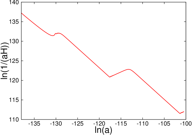
Figure 3: $\ln(a^{-1}H^{-1})$ versus $ln(a)$.

For appropriate choices of the constants the inflaton, $S$, lies along a flat direction denoted, which slowly rolls down in the potential obtained when the other fields take approximately constant values, $\phi\approx 0,\chi\approx 0$, close to their local minimum. The dynamics of $S$ field then triggers second order phase transition for $\phi$ and $\chi$ fields respectively. Let us assume that the vev of the inflaton is sufficiently large, $\langle S\rangle\sim M_{\rm p}$, such that

$$S>S_{c}=\sqrt{2}\left(\frac{\lambda_{1}}{\lambda_{2}}\right)\phi_{c}>\sqrt{2}\left(\frac{g_{1}}{g_{2}}\right)\chi_{c}\,.$$ (25)

With this choice, the fields $\phi$ and $\chi$ obtain large masses from the vev of $S$ and therefore they settle down in their local minimum given by $\phi=0$ and $\chi=0$. Their dynamics is then completely decoupled from that of $S$. The potential along the bottom of the trough parameterized by $S$ is then given approximately by $V\approx m^{2}S^{2}/2$. For values of $S\geq M_{p}$, the first phase of inflation is a chaotic type, which comes to an end when $S\sim M_{p}$. The $S$ field keeps rolling and when $S$ approaches $S_{c}$ the first phase transition occurs and then subsequently the third.

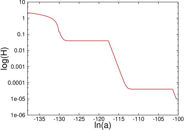
Figure 4: $\ln(H)$ versus $ln(a)$.

After the first phase of inflation the potential is dominated by the false vacuum of the $\phi$ field,

$$V\approx\lambda_{1}^{2}\phi_{c}^{4}+g_{1}^{2}\chi_{c}^{4}+\frac{1}{2}m^{2}S^{2}\approx\lambda_{1}^{2}\phi_{c}^{4}+\frac{1}{2}m^{2}S^{2}\,,$$ (26)

where the latter equality holds when $\lambda_{1}\phi_{c}^{2}\gg g_{1}\chi_{c}^{2}$.

Our potential is quite rich and depending on the choice of parameters many interesting possibilities can emerge. For the purpose of demonstration how the multiple inflation works, we have studied the evolution of fields in an expanding universe with these set of parameters and initial conditions; $s_{0}=3.0M_{p},\ \phi_{0}=0,\ \chi_{0}=0$, $\phi_{c}=\chi_{c}=0.2~{}M_{p}$, $m=1.0~{}M_{p},\ \lambda_{1}=1,\ \lambda_{2}=1,\ g_{1}=0.001,\ g_{2}=1$. The vevs and masses are in Planck units. The resulting dynamics and expansion are shown in Figs.(3,4,5).

For the above choice of parameters the inflaton field slow rolls until its vev becomes of order the Planck scale. This is the first phase of inflation. During this period $\ln(H^{-1}/a)$ decreases as shown in Fig. (3). After inflation the $S$ field rolls fast towards its minimum and on its way down it triggers the dynamics of $\phi$ and then $\chi$ field. The dynamics of $\chi$ field is triggered after $\phi$, which can be understood from eq. (25), though this is hard to see from the numerical plots. For a brief period the energy density of the Universe is dominated by the coherent oscillations of the $S$ field. On average these oscillations mimic an equation of state that of matter dominated epoch and the energy density redshifts as $a^{-3}$. During this period $\ln(H^{-1}/a)$ increases as $(1/3)\ln(t)$, this can be seen in Fig. (3) and in Fig. (5). The Hubble expansion rate drops which is depicted in Fig. (4).

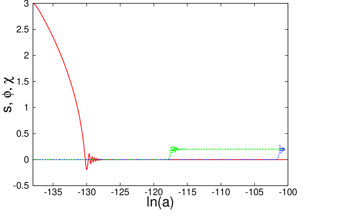
Figure 5: The field values $s,\phi,\chi$ plotted as function of $ln(a)$.

As the energy density stored in $S$ field redshifts it catches up with that of the false vacuum of $\phi$ field, and this is the onset of second bout of inflation. Note that in between the two epochs of inflation there is a possibility that some modes which left the horizon earlier during the first phase can be reprocessed as they enter the horizon during the second phase of inflation, see Fig. (2). This puts an interesting constraint on the number of $e$-foldings which we derived in our previous section. The dynamics of the $\phi$ field is quite interesting, when the $S$ field started rolling after the end of inflation it already displace the $\phi$ field from its local maximum due to presence of the coupling $g_{1}^{2}S^{2}\phi^{2}$. However $S$ rolls very slowly towards its global minimum, $\phi_{c}$. In this respect the second bout of inflation is due to slow rolling of the $\phi$ field, which is similar to the case where the second order phase transition happens extremely slowly studied earlier in ref. [25].

After the second bout of inflation the $\phi$ field oscillates coherently and its oscillations dominate the energy density of the Universe before being taken over by the false vacuum energy density of the $\chi$ field. During the $\phi$ oscillations the Universe enters briefly into a matter dominated epoch. This is shown in Fig. (3) as a second break in $\ln(H^{-1}/a)$. The oscillations of $\phi$ field can be seen in Fig. (5). The dynamical evolution of the Universe after this phase is solely determined by the potential created by the $\chi$ field. The Universe enters the third epoch of inflation, which is shown in Fig. (3,4). The comoving Hubble length decreases with time until $\chi$ begins its oscillations.

For other choice of parameters it is possible to show that the $S$ field keeps rolling while inflation occurs due to the false vacuum of $\phi$ field and then by $\chi$ field. These two fields decouple gradually from the dynamics followed by the $S$ field. The full dynamical analysis of this toy model will be given in a separate publication. It is a matter of simple extension that our model can predict several bouts of inflation one after the other followed by the epochs of matter domination.

It is tempting to try to embed this kind of construction into the scalar sector of the supergravity theories which have emerged recently within discussions of string-inspired inflationary models. This is of particular interest given the potentially natural occurrence there of string networks at the end of the first inflationary period.

Perhaps the simplest model of this type to consider is to imagine having an initial period of brane-antibrane inflation within a warped throat, perhaps along the lines of explicit models examined in refs. [9, 12]. The success of this inflationary epoch relies on fairly detailed tuning of the parameters of the inflaton potential, and this tuning would be less severe if only the 12 $e$-foldings of inflation found here were required.

Once the initial brane and antibrane have annihilated, their relative displacement is no longer available to be inflatons within the low-energy effective theory. A simple way to obtain a second inflationary phase could then be to use a bulk modulus as an inflaton, along the lines of the ‘racetrack’ inflationary mechanism [7]. This mechanism also requires fine-tuning of scalar parameters, although we have seen that only of order 20 $e$-foldings would be required for this second inflationary phase. It is an open question whether the fine-tunings required to obtain these two kinds of inflation can be made compatible with one another.

5 Conclusions

In a nutshell, our conclusions are these: A two-step inflationary process, with an initial inflationary scale of order $V_{I}^{1/4}\sim 10^{16}$ GeV and a subsequent scale of order $V_{II}^{1/4}\sim 10^{3}$ GeV, can take place without having observable effects on those fluctuations which are presently observable on cosmological scales. How much inflation is required during these two epochs turns out to depend crucially on the equation of state of the universe during the inter-inflationary phase, as follows.

• Requiring that the scales which are accessible to cosmological observations leave the horizon during the first inflationary period implies that this period must be at least 7 $e$-foldings long.

• The requirement that the universe expands enough to dilute the energy density from $V_{I}$ to $V_{II}$ ensures that an enormous amount of expansion occurs during the inter-inflationary phase. For most non-inflationary equations of state, many of the modes which leave the horizon by the end of the first inflationary epoch will re-enter the horizon between the inflationary epochs. For matter- or radiation-dominated equations of state the requirement that none of the observable modes get reprocessed in this way implies that there must be at least about 20 $e$-foldings of inflation between the exit of the last observable mode and the end of the first inflationary period.

• Solving the flatness and horizon problems of the late universe needs a total amount of inflation in both epochs of at least about 32 $e$-foldings. This number increases with the energy scale, $V_{II}$, of the second inflationary period.

• In the special case that the equation of state during the inter-inflationary phase is that of a cosmic string network, $p=-\rho/3$, the product $aH$ remains constant and modes neither enter nor leave the horizon during this phase. In this case modes sufficiently close to the horizon do get re-processed. In a simple model we find that that no observable effects for the CMB arise if there are around 5 $e$-foldings of inflation between the exit of the observable modes and the end of the first inflationary period. In this case only 7+5 = 12 $e$-foldings would be required during the first inflationary period, with a further 20 being required during the second inflationary epoch.

We have pursued this model as an example of the new and unexpected options presented to the inflationary model builder by the string landscape. The present analysis is a first pass at understanding the phenomenology of this two phase model of inflation, and relies on a number of simplifying assumptions in order to capture the basic physics of the model. Interestingly, while the use of two stages of inflation means that this model is much more complicated that many other inflationary scenarios, it does not depend on carefully tuned numerical coefficients. Indeed, the 10 or so $e$-folds of inflation at high scales is roughly the number one finds in the absence of tuning for broad classes of inflationary models. Likewise, the 25 $e$-folds of inflation needed at the TeV scale for the particular example we consider here is natural in some contexts, such as locked inflation [15, 16]. Moreover, since the second period of inflation does not produce the density perturbations we see on the sky, we could imagine it being produced by a much broader range of mechanisms or potentials than we could normally consider.

6 Appendix

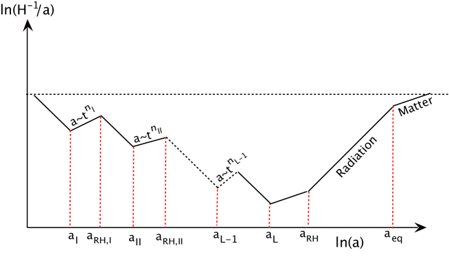
Figure 6: A sketch of the comoving Hubble scale during a multi-step inflationary process. We plotted $\ln(H^{-1}/a)$ versus $\ln(a)$. We assumed inflationary epochs are followed by normal power law expnasions with $n_{1},n_{2},..,n_{L}\leq 1$. We also assume that after the final bout of inflation the Universe is finally settled in a radiation and then in a matter dominated epoch.

We present a scenario where there are mutiple stages of inflation one after the other separated by the matter epochs, whose expansions are parameterized by $t^{n_{1}},~{}t^{n_{2}},...,~{}t^{n_{L}}$, with $n_{1},~{}n_{2},...,n_{L}\leq 1$. We define the $e$-foldings during the $L$ different inflationary periods as

$$\textrm{e}^{N_{I}(k)}\equiv{a_{I}\over a_{k}},\ \ \textrm{e}^{N_{i}}\equiv{a_{i}\over a_{RH,i-1}},\ i=2,3,...,L\,,$$ (27)

where $a_{i}$ is the value of the scale factor during the end of the $i$th phase of inflation and $a_{RH,i}$ during the end of the $i$th reheating period.

In addition, we define the number of $e$-foldings of expansion when the critical scale leaves the horizon before the end of first inflationary period

$$\textrm{e}^{\widetilde{N}}\equiv{a_{I}\over a_{k_{c}}}\,.$$ (28)

It is now straightforward to generalize eq. (3):

$${k\over a_{0}H_{0}} = {a_{k}H_{k}\over a_{0}H_{0}}$$

$$= \Big{(}{a_{k}\over a_{I}}\Big{)}\Big{(}{a_{I}\over a_{RH,I}}\Big{)}\Big{(}{a_{RH,I}\over a_{II}}\Big{)}\Big{(}{a_{II}\over a_{RH,II}}\Big{)}...\Big{(}{a_{RH,L-1}\over a_{L}}\Big{)}\Big{(}{a_{L}\over a_{RH}}\Big{)}\Big{(}{a_{RH}\over a_{eq}}\Big{)}\Big{(}{H_{k}\over H_{eq}}\Big{)}\Big{(}{a_{eq}H_{eq}\over a_{0}H_{0}}\Big{)}$$

$$= \textrm{e}^{-N_{I}(k)}\Big{(}{a_{I}\over a_{RH,I}}\Big{)}\textrm{e}^{-N_{II}}\Big{(}{a_{II}\over a_{RH,II}}\Big{)}...e^{-N_{L}}\Big{(}{\rho_{L}\over\rho_{RH}}\Big{)}^{-1/3}\Big{(}{\rho_{RH,II}\over\rho_{eq}}\Big{)}^{-1/4}\Big{(}{H_{k}\over H_{eq}}\Big{)}\Big{(}{a_{eq}H_{eq}\over a_{0}H_{0}}\Big{)}\,.$$

Since during the period between $i$ and $i+1$ phases of inflation, the Universe expands as $a\sim t^{n}_{i}$. Hence during these periods, $\ln(1/(aH))\sim(1-n_{i})/n_{i}\ln(a)$, and therefore

$$\ln\Big{(}{a_{i}\over a_{RH,i}}\Big{)}={n_{i}\over 2}\ln\Big{(}{V_{i+1}\over V_{i}}\Big{)}\,.$$ (30)

Substituting eq. (30) into eq. (6), and a careful rearrangement gives

$$N_{I}(k)+\sum_{i=2}^{L}N_{i} = -\ln\Big{(}{k\over a_{0}H_{0}}\Big{)}+\frac{1}{3}\ln\Big{(}{\rho_{RH,L}\over\rho_{L}}\Big{)}+\frac{1}{4}\ln\Big{(}{\rho_{eq}\over\rho_{RH,L}}\Big{)}$$ (31)

$$+\ln\Big{(}{\sqrt{8\pi V_{k}\over 3m_{Pl}^{2}}{1\over H_{eq}}}\Big{)}+\ln(219\,\Omega_{0}h)+\sum_{i=1}^{L-1}{n_{i}\over 2}\ln\Big{(}{V_{i+1}\over V_{i}}\Big{)}\,.$$

We can assume instant reheating after the last phase of inflation, which yields, $\rho_{L,end}=\rho_{RH,L}$. Concentrating on the present horizon scale (we define $N_{I}\equiv N_{I}(a_{0}H_{0})$), we find

$$\sum_{i=1}^{L}N_{i}=68.5+\frac{1}{4}\ln\Big{(}{V^{2}_{I}\over V_{L}m_{Pl}^{4}}\Big{)}+\sum_{i=1}^{L-1}{n_{i}\over 2}\ln\Big{(}{V_{i+1}\over V_{i}}\Big{)}\,.$$ (32)

In comparison to the two-stage inflationary epochs, there is now a set of constraints arising from the fact that there should be no reprocessing of modes on the scales probed by CMB experiments. This requirement constraints

$$\ln\Big{(}{1\over a_{k_{c}}H_{I}}\Big{)}>\ln\Big{(}{1\over a_{RH,i}H_{i+1}}\Big{)}\,,\ \ i=2,...,L-1\,$$ (33)

or,

$$\ln\Big{(}{a_{RH,i}\over a_{k_{c}}}\Big{)}>\frac{1}{2}\ln\Big{(}{V_{I}\over V_{i+1}}\Big{)}\,,\ \ i=2,...,L-1\,.$$ (34)

The left hand side can be expanded:

$$\ln\Big{(}{a_{RH,i}\over a_{k_{c}}}\Big{)} = \ln\Big{(}{a_{I}\over a_{k_{c}}}{a_{RH,I}\over a_{I}}{a_{II}\over a_{RH,I}}...{a_{RH,i}\over a_{i}}\Big{)}$$ (35)

$$= \widetilde{N}-{n_{1}\over 2}\ln\Big{(}{V_{II}\over V_{I}}\Big{)}+N_{II}-{n_{2}\over 2}\ln\Big{(}{V_{III}\over V_{II}}\Big{)}+...+N_{i}-{n_{i}\over 2}\ln\Big{(}{V_{i+1}\over V_{i}}\Big{)}$$

$$= \widetilde{N}+\sum_{j=2}^{i}N_{j}-\sum_{j=1}^{i}{n_{j}\over 2}\ln\Big{(}{V_{i+1}\over V_{i}}\Big{)}$$

$$= \frac{1}{2}\ln\Big{(}{V_{I}\over V_{II}}\Big{)}+\sum_{j=2}^{i}N_{j}+\sum_{j=2}^{i}{n_{j}\over 2}\ln\Big{(}{V_{i}\over V_{i+1}}\Big{)}\,,$$

where in the last step we have used $\widetilde{N}=(1-n_{1})/2\ln(V_{I}/V_{II})$.

Hence, in general we obtain the following set of constraints:

$$N_{I}>6.9+{1-n_{1}\over 2}\ln\Big{(}{V_{I}\over V_{II}}\Big{)}$$

$$\sum_{j=2}^{i}N_{j}>\frac{1}{2}\ln\Big{(}{V_{II}\over V_{i+1}}\Big{)}-\sum_{j=2}^{i}{n_{j}\over 2}\ln\Big{(}{V_{i}\over V_{i+1}}\Big{)}\,,\ \ i=2,...,L-1\,.$$ (36)

In the special case $n_{i}=1$, it is easy to see that these constraints are trivially satisfied ($\sum_{j}N_{j}>0$).

References

- [1] G. R. Dvali and S. H. H. Tye, “Brane inflation,” Phys. Lett. B 450 (1999) 72 (hep-ph/9812483).
- [2] C. P. Burgess, M. Majumdar, D. Nolte, F. Quevedo, G. Rajesh and R. J. Zhang, “The inflationary brane-antibrane universe,” JHEP 0107 (2001) 047 (hep-th/0105204).
- [3] G. R. Dvali, Q. Shafi and S. Solganik, “D-brane inflation,” [hep-th/0105203]; S. Alexander, Inflation from D-anti-D brane annihilation, hep-th/0105032, A. Mazumdar, S. Panda and A. Perez-Lorenzana, “Assisted inflation via tachyon condensation,” Nucl. Phys. B 614 (2001) 101 [hep-ph/0107058].
- [4] J. Garcia-Bellido, R. Rabadan and F. Zamora, “Inflationary scenarios from branes at angles,” JHEP 0201, 036 (2002); N. Jones, H. Stoica and S. H. H. Tye, “Brane interaction as the origin of inflation,” JHEP 0207, 051 (2002); M. Gomez-Reino and I. Zavala, “Recombination of intersecting D-branes and cosmological inflation,” JHEP 0209, 020 (2002).
- [5] C. Herdeiro, S. Hirano and R. Kallosh, “String theory and hybrid inflation / acceleration,” JHEP 0112 (2001) 027 [hep-th/0110271]; K. Dasgupta, C. Herdeiro, S. Hirano and R. Kallosh, “D3/D7 inflationary model and M-theory,” Phys. Rev. D 65 (2002) 126002 [hep-th/0203019]. J. P. Hsu, R. Kallosh and S. Prokushkin, “On brane inflation with volume stabilization,” JCAP 0312 (2003) 009 [hep-th/0311077]; R. Kallosh and S. Prokushkin, “SuperCosmology,” [hep-th/0403060]; J. P. Hsu and R. Kallosh, “Volume stabilization and the origin of the inflaton shift symmetry in string theory,” JHEP 0404 (2004) 042 [hep-th/0402047];
- [6] C. P. Burgess, P. Martineau, F. Quevedo, G. Rajesh and R. J. Zhang, “Brane antibrane inflation in orbifold and orientifold models,” JHEP 0203 (2002) 052 [hep-th/0111025]; L. Pilo, A. Riotto and A. Zaffaroni, “Old inflation in string theory,” [hep-th/0401004]; F. Koyama, Y. Tachikawa and T. Watari, “Supergravity analysis of hybrid inflation model from D3-D7 system”, [hep-th/0311191]; H. Firouzjahi and S. H. H. Tye, “Closer towards inflation in string theory,” Phys. Lett. B 584 (2004) 147 [hep-th/0312020]. S. Buchan, B. Shlaer, H. Stoica and S. H. H. Tye, “Inter-brane interactions in compact spaces and brane inflation,” [hep-th/0311207]; C. Escoda, M. Gomez-Reino and F. Quevedo, “Saltatory de Sitter string vacua,”JHEP 0311 (2003) 065, [hep-th/0307160]; C. P. Burgess, R. Kallosh and F. Quevedo, “de Sitter string vacua from supersymmetric D-terms,” JHEP 0310 (2003) 056 [hep-th/0309187] A. Buchel and R. Roiban, “Inflation in warped geometries,” hep-th/0311154; H. Firouzjahi and S. H. H. Tye, “Closer towards inflation in string theory,” [hep-th/0312020]; A. Saltman and E. Silverstein, “The Scaling of the No Scale Potential and de Sitter Model Building,” [hep-th/0402135]; E. Halyo, “D-brane inflation on conifolds,” hep-th/0402155; M. Becker, G. Curio and A. Krause, Nucl. Phys. B693 (2004) 223-260 [hep-th/0403027]; M. Alishahiha, E. Silverstein and D. Tong, “DBI in the sky,” (hep-th/0404084); O. DeWolfe, S. Kachru and H. Verlinde, “The giant inflaton,” JHEP 0405 (2004) 017 [hep-th/0403123]; N. Iizuka and S. P. Trivedi, “An inflationary model in string theory,” [hep-th/0403203]; A. Buchel and A. Ghodsi, “Braneworld inflation,” Phys. Rev. D 70 (2004) 126008 [hep-th/0404151]; M. Berg, M. Haack and B. Kors, “Loop corrections to volume moduli and inflation in string theory,” Phys. Rev. D 71 (2005) 026005 [hep-th/0404087]; M. Berg, M. Haack and B. Kors, “On the moduli dependence of nonperturbative superpotentials in brane inflation,” [hep-th/0409282]; K. Maeda and N. Ohta, “Inflation from M-Theory with Fourth-order Corrections and Large Extra Dimensions”, Phys. Lett. B 597 (2004) 400, [hep-th/0405205]; K. Maeda and N. Ohta, “Inflation from Superstring/M Theory Compactification with Higher Order Corrections I ”, [hep-th/0411093]; N. Ohta, “Accelerating Cosmologies and Inflation from M/superstring Theories”, [hep-th/0411230]; X. Chen, “Multithroat brane inflation”, [hep-th/0408084].
- [7] J.J. Blanco-Pillado, C.P. Burgess, J.M. Cline, C. Escoda, M. Gómez-Reino, R. Kallosh, A. Linde, and F. Quevedo, “Racetrack Inflation,” [hep-th/0406230].
- [8] F. Quevedo, Class. Quant. Grav. 19 (2002) 5721, [hep-th/0210292]; A. Linde, “Prospects of inflation,” [hep-th/0402051].
- [9] S. Kachru, R. Kallosh, A. Linde and S. P. Trivedi, “de Sitter Vacua in String Theory,” [hep-th/0301240]; S. Kachru, R. Kallosh, A. Linde, J. Maldacena, L. McAllister and S. P. Trivedi, “Towards inflation in string theory,” JCAP 0310 (2003) 013 [hep-th/0308055].
- [10] S. B. Giddings, S. Kachru and J. Polchinski, “Hierarchies from fluxes in string compactifications,” Phys. Rev. D66, 106006 (2002).
- [11] S. Sethi, C. Vafa and E. Witten, “Constraints on low-dimensional string compactifications,” Nucl. Phys. B 480 (1996) 213 [hep-th/9606122]; K. Dasgupta, G. Rajesh and S. Sethi, “M theory, orientifolds and G-flux,” JHEP 9908 (1999) 023 [hep-th/9908088].
- [12] C. P. Burgess, J. M. Cline, H. Stoica and F. Quevedo, “Inflation in realistic D-brane models,” [hep-th/0403119].
- [13] G. D. Coughlan, W. Fischler, E. W. Kolb, S. Raby and G. G. Ross, “Cosmological Problems For The Polonyi Potential,” Phys. Lett. B 131 (1983) 59; B. de Carlos, J. A. Casas, F. Quevedo and E. Roulet, “Model independent properties and cosmological implications of the dilaton and moduli sectors of 4-d strings,” Phys. Lett. B 318 (1993) 447 [hep-ph/9308325]; T. Banks, D. B. Kaplan and A. E. Nelson, “Cosmological implications of dynamical supersymmetry breaking,” Phys. Rev. D 49 (1994) 779 [hep-ph/9308292].
- [14] R. Easther, “Folded Inflation, Primordial Tensors and the Running of the Scalar Spectral Index,” [hep-th/0407042].
- [15] G. Dvali and S. Kachru, “New old inflation,” hep-th/0309095.
- [16] R. Easther, J. Khoury and K. Schalm, “Tuning locked inflation: Supergravity versus phenomenology,” JCAP 0406, 006 (2004) [hep-th/0402218].
- [17] D. H. Lyth and E. D. Stewart, “Thermal inflation and the moduli problem,” Phys. Rev. D 53, 1784 (1996) [hep-ph/9510204].
- [18] J. Silk and M.S. Turner, Phys. Rev. D35 (1987) 419; R. Holman, E.W. Kolb, S.L. Vadas and Y. Wang, Phys. Lett. B269 (1991) 252-256; D. Polarski and A.A. Starobinsky, Nucl. Phys. B385 (1992) 623-650; J.A. Adams, G.G. Ross and S. Sarkar, Nucl. Phys. B503 (1997) 405-425 [hep-ph/9704286]; G. Lazarides and N. Tetradis, Phys. Rev. D58 (1998) 123502 [hep-ph/9802242]; T. Kanazawa, M. Kawasaki, N. Sugiyama and T. Yanagida, Phys. Rev. D61 (2000) 023517 [hep-ph/9908350]; T. Kanazawa, M. Kawasaki and T. Yanagida, Phys. Lett. B482 (2000) 174-182 [hep-ph/0002236]; M. Yamaguchi, Phys. Rev. D64 (2001) 063502 [hep-ph/0103045]; Phys. Rev. D64 (2001) 063503 [hep-ph/0105001]; D. Parkinson, S. Tsujikawa, B.A. Bassett and L. Amendola, [astro-ph/0409071].
- [19] A. D. Linde, “Eternal Chaotic Inflation,” Mod. Phys. Lett. A 1, 81 (1986); A. A. Starobinsky, in Current Topics in Field Theory, Quantum Gravity and Strings, eds. H. J. Vega and N. Sanchez, Lecture Notes in Physics 206, Springer, Heidelberg (1996); A. D. Linde and A. Mezhlumian, “Stationary universe,” Phys. Lett. B 307, 25 (1993) [gr-qc/9304015]; A. Vilenkin, “Making predictions in eternally inflating universe,” Phys. Rev. D 52, 3365 (1995) [gr-qc/9505031]; A. H. Guth, “Inflation and eternal inflation,” Phys. Rept. 333, 555 (2000) [astro-ph/0002156].
- [20] A. R. Liddle and S. M. Leach, Phys. Rev. D68, 103503 (2003).
- [21] A. R. Liddle and D. H. Lyth, Cosmological Inflation and Large-Scale Structure, Cambridge University Press (2000).
- [22] S. Sarangi and S. H. H. Tye, “Cosmic string production towards the end of brane inflation,” Phys. Lett. B 536 (2002) 185 [hep-th/0204074]; G. Dvali, R. Kallosh and A. Van Proeyen, “D-term strings,” JHEP 0401 (2004) 035 [hep-th/0312005]; G. Dvali and A. Vilenkin, “Formation and evolution of cosmic D-strings,” JCAP 0403 (2004) 010 [hep-th/0312007].
- [23] E. J. Copeland, R. C. Myers and J. Polchinski, “Cosmic F- and D-strings,” JHEP 0406 (2004) 013 [hep-th/0312067]; L. Leblond and S. H. H. Tye, “Stability of D1-strings inside a D3-brane,” JHEP 0403 (2004) 055 [hep-th/0402072]; K. Dasgupta, J. P. Hsu, R. Kallosh, A. Linde and M. Zagermann, “D3/D7 brane inflation and semilocal strings,” [hep-th/0405247].
- [24] J. Garcia-Bellido, A. D. Linde and D. Wands, “Density perturbations and black hole formation in hybrid inflation,” Phys. Rev. D 54, 6040 (1996) [astro-ph/9605094].
- [25] A. M. Green and A. Mazumdar, “Dynamics of a large extra dimension inspired hybrid inflation model,” Phys. Rev. D 65, 105022 (2002) [hep-ph/0201209], A. Mazumdar,“Low scale inflation with large number of -foldings,” [hep-th/0310162].
- [26] M. B. Green, J. H. Schwarz, Phy. Lett. B 149, 117 (1984).
- [27] G. V. Chibisov and V. F. Mukhanov, “Galaxy Formation And Phonons,” Mon. Not. Roy. Astron. Soc. 200, 535 (1982); V. F. Mukhanov, “Quantum Theory Of Gauge Invariant Cosmological Perturbations,” Sov. Phys. JETP 67 (1988) 1297 [Zh. Eksp. Teor. Fiz. 94N7 (1988) 1]; V. F. Mukhanov, H. A. Feldman and R. H. Brandenberger, “Theory of cosmological perturbations”, Phys. Rep. 215 (1992) 203; E. D. Stewart and D. H. Lyth, “A More accurate analytic calculation of the spectrum of cosmological perturbations produced during inflation,” Phys. Lett. B 302, 171 (1993) [gr-qc/9302019].
- [28] A. Albrecht and N. Turok, Phys. Rev. Lett. 54 (1985) 1868; M. Aryal, A.E. Everett, A. Vilenkin and T. Vachaspati, Phys. Rev. D34 (1986) 434-439; E.J. Copeland and N. Turok, FERMILAB-PUB-86-127-A, Sep 1986.; E.P.S. Shellard, Nucl. Phys. B283 (1987) 624-656; R.H. Brandenberger, Nucl. Phys. B293 (1987) 812; D.P. Bennett and F.R. Bouchet, Phys. Rev. Lett. 60 (1988) 257; M. Hindmarsh, A.C. Davis and R.H. Brandenberger, Phys. Rev. D49 (1994) 1944-1950 [hep-ph/9307203]; R. H. Brandenberger and A. C. Davis, Phys. Lett. B 332, 305 (1994) [hep-ph/9403269]; N. Barnaby, A. Berndsen, J. M. Cline and H. Stoica, “Overproduction of cosmic superstrings,” [hep-th/0412095]; P.P. Avelino, R.R. Caldwell, C.J.A.P. Martins, “Cosmic strings in an open universe: quantitative evolution and observational consequences,” Phys. Rev. D 56 (1997) 4568.
- [29] A. Vilenkin, Phys. Rep. 121 (1985) 263; N. Turok, in Particles, Strings and Supernovae, ed. by. A. Jevicki and C.I. Tan, World Scientific, Singapore, 1989;
- [30] T.W.B. Kibble, J. Phys. A9 (1976) 1387; Phys. Rep. 67 (1980) 183.