Scale-dependent stochastic quantization

Abstract

Based on the wavelet-defined multiscale random noise proposed in [2], a multiscale version of the stochastic quantization procedure is considered. A new type of the commutation relations emerging from the multiscale decomposition of the operator-valued fields is derived.

1 Introduction

A highly original method of stochastic quantization of gauge fields proposed by G.Parisi and Y.Wu [1] have been attracting attention for more than 20 years. Let $S_{E}[\phi]$ be the action Euclidean field theory in $\mathbb{R}^{d}$. Then, instead of direct calculation of the Green functions from the generation functional of the field theory, it is possible to introduce a fictitious time variable $\tau$, make the quantum fields into stochastic fields $\phi(x)\to\phi(x,\tau),x\!\in\!\mathbb{R}^{d},\tau\!\in\!\mathbb{R}$ and evaluate the moments $\langle\phi(x_{1},\tau_{1})\ldots\phi(x_{m},\tau_{m})\rangle$ by averaging over a random process $\phi(x,\tau,\cdot)$ governed by the Langevin equation

$$\frac{\partial\phi(x,\tau)}{\partial\tau}+\frac{\delta S}{\delta\phi(x,\tau)}=\eta(x,\tau).$$ (1)

The Gaussian random force is $\delta$-correlated in both the $\mathbb{R}^{d}$ coordinate and the fictitious time:

$$\langle\eta(x,\tau)\eta(x^{\prime},\tau^{\prime})\rangle=2D_{0}\delta(x-x^{\prime})\delta(\tau-\tau^{\prime}),\quad\langle\eta(x,\tau)\rangle=0.$$ (2)

The physical Green functions are obtained by taking the steady state limit

$$G(x_{1},\ldots,x_{m})=\lim_{\tau\to\infty}\langle\phi(x_{1},\tau)\ldots\phi(x_{m},\tau)\rangle.$$

Following [3] we extend the method of stochastic quantization by introducing the scale-dependent random processes $W(a,b,\cdot)$, where $b\in\mathbb{R}^{d}$ is a spatial coordinate, and $a$ is the spatial resolution. For a square-integrable function $f(x,\cdot)$ the wavelet coefficients are

$$W(a,{b},\cdot)=\int|a|^{-d}\overline{\psi\left(\frac{x-b}{a}\right)}f(x,\cdot)d^{d}x.$$ (3)

Hereafter they will be referred to as the scale components of $f$ with respect to the basic wavelet $\psi$. The reconstruction of a function from its scale components is given by the inverse wavelet transform

$$f(x,\cdot)=\frac{2}{C_{\psi}}\int_{0}^{\infty}\frac{da}{a^{d+1}}\int d^{d}b\psi\left(\frac{x-b}{a}\right)W(a,b,\cdot),\quad C_{\psi}=\int\frac{|\tilde{\psi}(k)|^{2}}{S_{d}|k|^{d}}d^{d}k,$$ (4)

with $S_{d}$ being the are of the unit sphere in $d$ dimensions, is the normalization for the isotropic wavelets. Performing the wavelet transform (in spatial coordinate) of the fields and the random force in the Langevin equation, we get the possibility to substitute the white noise (2) by a scale-dependent random force

$$\langle\tilde{\eta}(a_{1},k_{1},\tau_{1})\tilde{\eta}(a_{2},k_{2},\tau_{2})\rangle=C_{\psi}(2\pi)^{d}\delta^{d}(k_{1}+k_{2})\delta(\tau_{1}-\tau_{2})a_{1}\delta(a_{1}-a_{2})D(a_{1},k_{1})$$ (5)

In case the spectral density of the random force is a constant $D(a_{1},k_{1})=D_{0}$, the inverse wavelet transform

$$\phi(x)=\frac{2}{C_{\psi}}\int_{0}^{\infty}\frac{da}{a}\int\frac{d^{d}{k}}{(2\pi)^{d}}\frac{d\omega}{2\pi}\exp(\imath(kx-\omega\tau))\tilde{\psi}(ak)\tilde{\phi}(a,k,\omega),$$ (6)

drives the process (5) into the white noise (2).

In case of arbitrary functions $\phi(a,x,\cdot)$ we have more possibilities. In particular, we can define a narrow band forcing that acts at a single scale

$$D(a,k)=a_{0}\delta(a-a_{0})D_{0}.$$ (7)

The contribution of the scales with the wave vectors apart from the the typical scale $a_{0}^{-1}$ is suppressed by rapidly vanishing wings of the compactly supported wavelet $\tilde{\psi}(k)$.

Here we present two examples of the divergence free stochastic perturbation expansion: (i) the scalar field theory $\phi^{3}$, (ii) the non-Abelian gauge field theory.

2 Scalar field theory

Let us turn to the stochastic quantization of the $\phi^{3}$ theory with the scale-dependent noise [3]. The Euclidean action of the $\phi^{3}$ theory is

$$S_{E}[\phi(x)]=\int d^{d}x\left[\frac{1}{2}(\partial\phi)^{2}+\frac{m^{2}}{2}\phi^{2}+\frac{\lambda}{3!}\phi^{3}\right].$$ (8)

The corresponding Langevin equation is written as

$$\frac{\partial\phi(x,\tau)}{\partial\tau}+\left(-\Delta\phi+m^{2}\phi+\frac{\lambda}{2!}\phi^{2}\right)=\eta(x,\tau).$$ (9)

Substituting the scale components in representation (6) we get the integral equation for the stochastic fields

$$\begin{array}[]{l}(-\imath\omega+k^{2}+m^{2})\phi(a,k,\omega)=\eta(a,k,\omega)-\frac{\lambda}{2}\overline{\tilde{\psi}(ak)}\left(\frac{2}{C_{\psi}}\right)^{2}\int\frac{d^{d}{k_{1}}}{(2\pi)^{d}}\frac{d\omega_{1}}{2\pi}\frac{d{a_{1}}}{{a_{1}}^{{d}+1}}\frac{d{a_{2}}}{{a_{2}}^{{d}+1}}\\ \tilde{\psi}(a_{1}k_{1})\tilde{\psi}(a_{2}(k-k_{1}))\phi(a_{1},k_{1},\omega_{1})\phi(a_{2},k-k_{1},\omega-\omega_{1}).\end{array}$$ (10)

Starting from the zero-th order approximation $\phi_{0}=G_{0}\eta$ with the bare Green function $G_{0}(k,\omega)=1/(-\imath\omega+k^{2}+m^{2})$ and iterating the integral equation (10), we get the one-loop correction to the stochastic Green function

$$G(k,\omega)=G_{0}(k,\omega)+\lambda^{2}G_{0}^{2}(k,\omega)\int\frac{d^{d}{q}}{(2\pi)^{d}}\frac{d\Omega}{2\pi}2\Delta(q)|G_{0}(q,\Omega)|^{2}G_{0}(k-q,\omega-\Omega)+\ldots,$$ (11)

where $\Delta(k)$ is the scale averaged effective force correlator

$$\Delta(k)\equiv\frac{2}{C_{\psi}}\int_{0}^{\infty}\frac{da}{a}|\hat{\psi}(ak)|^{2}D(a,k).$$ (12)

In the same way the other stochastic momenta can be evaluated. Thus the common stochastic diagram technique is reproduced with the scale-dependent random force (5) instead of the standard one (2). The 1PI diagrams corresponding to the stochastic Green function decomposition (11) are shown in Fig. 1.

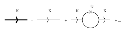
Figure 1: Diagram expansion of the stochastic Green function in $\phi^{3}$-model

It can be easily seen that for a single-band forcing (7) and a suitably chosen wavelet the loop divergences are suppressed. For instance, the use of the Mexican hat wavelet

$$\hat{\psi}(k)=(2\pi)^{d/2}(-\imath k)^{2}\exp(-k^{2}/2),\quad C_{\psi}=(2\pi)^{d}$$ (13)

for the single band random force (7) gives the effective force correlator

$$\Delta({q})=(a_{0}q)^{4}e^{-(a_{0}q)^{2}}D_{0}.$$ (14)

The loop integrals taken with this effective force correlator (14) can be easily seen to be free of ultra-violet divergences

$$G_{2}(k,\omega) = G_{0}^{2}(k,\omega)\int\frac{d^{d}{q}}{(2\pi)^{d}}2\Delta(q)\int_{-\infty}^{\infty}\frac{d\Omega}{2\pi}\frac{1}{\Omega^{2}+(q^{2}+m^{2})^{2}}$$ (15)

$$\times \frac{1}{-\imath(\omega-\Omega)+(k-q)^{2}+m^{2}}$$

3 Non-Abelian gauge theory

The Euclidean action of a non-Abelian field is given by

$$S[A]=\frac{1}{4}\int d^{d}xF_{\mu\nu}^{a}(x)F_{\mu\nu}^{a}(x),\quad F_{\mu\nu}^{a}(x)=\partial_{\mu}A_{\nu}^{a}(x)-\partial_{\nu}A_{\mu}^{a}(x)+gf^{abc}A_{\mu}^{b}(x)A_{\nu}^{c}(x).$$ (16)

The Langevin equation for the gauge theory (16) can be written as

$$\frac{\partial A_{\mu}^{a}(x,\tau)}{\partial\tau}+\bigl{(}-\delta_{\mu\nu}\partial^{2}+\partial_{\mu}\partial_{\nu}\bigr{)}A_{\nu}^{a}(x,\tau)=\eta_{\mu}^{a}(x,\tau)+U_{\mu}^{a}(x,\tau),$$ (17)

where $\eta_{\mu}^{a}(x,\tau)$ is the random force and $U_{\mu}^{a}(x,\tau)$ is the nonlinear interaction term

$$U[A]=\frac{g}{2}V^{0}(A,A)+\frac{g^{2}}{6}W^{0}(A,A,A).$$

The stochastic diagram technique for the gauge field Langevin equation (17) is summarized in the Table 1.

Table 1: Stochastic diagrams for the non-Abelian gauge fields. Redrawn from [4]

Diagram	Notation	Formula
	$G_{\mu\nu}^{ab}(k,\tau-\tau^{\prime})$	$\delta^{ab}\theta(\tau-\tau^{\prime})\left[\left(\delta_{\mu\nu}-\frac{k_{\mu}k_{\nu}}{k^{2}}\right)e^{-k^{2}(\tau-\tau^{\prime})}+\frac{k_{\mu}k_{\nu}}{k^{2}}\right]$
	$D_{\mu\nu}^{ab}(k,\tau-\tau^{\prime})$	$\delta^{ab}\Bigl{[}\left(\delta_{\mu\nu}-\frac{k_{\mu}k_{\nu}}{k^{2}}\right)\bigl{(}e^{-k^{2}|\tau-\tau^{\prime}|}-e^{-k^{2}(\tau+\tau^{\prime})}\bigr{)}$
		$+2min(\tau,\tau^{\prime})\frac{k_{\mu}k_{\nu}}{k^{2}}+\frac{k_{\mu}k_{\nu}}{k^{2}}\Bigr{]}$
	$\frac{g}{2}V_{\mu\kappa\lambda}^{abc}(k_{1},k_{2},k_{3})$	$\frac{\imath g}{2}f^{abc}\bigl{[}(k_{1}-k_{2})_{\lambda}\delta_{\mu\kappa}+(k_{2}-k_{3})_{\mu}\delta_{\kappa\lambda}$
		$+(k_{3}-k_{1})_{\kappa}\delta_{\mu\lambda}\bigr{]}$
	$\frac{g^{2}}{6}W_{\mu\nu\kappa\lambda}^{abcd}$	$-\frac{g^{2}}{6}\bigl{[}f^{xab}f^{xcd}(\delta_{\mu\kappa}\delta_{\nu\lambda}-\delta_{\mu\lambda}\delta_{\nu\kappa})$
		$+f^{xac}f^{xbd}(\delta_{\mu\nu}\delta_{\kappa\lambda}-\delta_{\mu\lambda}\delta_{\nu\kappa})$
		$+f^{xad}f^{xbc}(\delta_{\mu\nu}\delta_{\kappa\lambda}-\delta_{\mu\kappa}\delta_{\nu\lambda})\bigr{]}$

The two terms standing in the free field Green function correspond to the transversal and the longtitudal mode propagation:

$$G_{\mu\nu}^{ab}(k)=\frac{T_{\mu\nu}(k)\delta_{ab}}{-\imath\omega+k^{2}}+\frac{L_{\mu\nu}(k)\delta_{ab}}{-\imath\omega},\qquad T_{\mu\nu}(k)=\delta_{\mu\nu}-\frac{k_{\mu}k_{\nu}}{k^{2}},L_{\mu\nu}(k)=\frac{k_{\mu}k_{\nu}}{k^{2}}.$$

(Here we are concerned with divergences and do not touch any gauge fixing.)

Similarly the scalar field theory, we can use the scale-dependent forcing (18) in the Langevin equation (17). Since there is no dynamic evolution for the longtitudal modes in the Langevin equation (17), it is natural to use the transversal scale-dependent random force

$$\langle\eta_{\mu}^{a}(a_{1},k_{1},\tau_{1})\eta_{\nu}^{b}(a_{2},k_{2},\tau_{2})\rangle = (2\pi)^{d}\delta^{d}(k_{1}+k_{2})\delta(\tau_{1}-\tau_{2})T_{\mu\nu}(k_{1})$$ (18)

$$\times C_{\psi}a_{1}\delta(a_{1}-a_{2})D(a_{1},k_{1}).$$

Let us consider a gluon loop with two cubic vertices. Summing up over the gauge group indices $\bigl{(}\frac{\imath}{2}g\bigr{)}^{2}f^{abc}\delta_{bd}f^{der}\delta_{cr}=\frac{g^{2}}{4}\delta_{ae}C_{2},$ with $C_{2}=N$ for $SU_{N}$ groups, we can wright the gluon loop as a sum of two diagrams – those with the transversal and the longtitudal stochastic Green functions

$$G_{2\mu\nu}^{ab}(k,\omega)=g^{2}\delta_{ab}C_{2}|G_{0}(k,\omega)|^{2}\sum_{I=T,L}\int\frac{d\Omega}{2\pi}\frac{d^{d}{q}}{(2\pi)^{d}}N^{I}(k,\omega,q,\Omega)l^{I}_{\mu\nu}(k,q)2\Delta(q)$$ (19)

where

$$N(k,q)=\left|\frac{1}{-\imath\Omega+q^{2}}\right|^{2}\begin{pmatrix}\frac{1}{-\imath(\omega-\Omega)+(k-q)^{2}}\cr\frac{1}{-\imath(\omega-\Omega)}\end{pmatrix}$$

$$l_{\mu\nu}(k,q)=V_{\mu\kappa\lambda}(k,k-q,q)T_{\lambda\gamma}(q)V_{\sigma\nu\gamma}(k-q,k,-q)\begin{pmatrix}T_{\kappa\sigma}(k-q)\cr L_{\kappa\sigma}(k-q)\end{pmatrix}$$

As it can be observed after explicit evaluation of the tensor structures $l^{T}_{\mu\nu}$ and $l^{L}_{\mu\nu}$, and integration over $d\Omega$, the wavelet factor in the effective force correlator $\Delta(q)$ will suppress the divergences for a narrow-band forcing (7). The power factor $k^{n}$ of the basic wavelet $\psi$, that provides $\tilde{\psi}(0)=0$, also makes the IR behavior softer. In this respect the wavelet regularization is different from the continuous regularization $\int d^{d}yR_{\Lambda}(\partial^{2})\eta(y,\tau)$, see e.g. [6], that makes UV behavior softer by the factor $e^{-\frac{k^{2}}{\Lambda^{2}}}$, but do not affect the IR behavior.

4 Commutation relation

The stochastic quantization with a forcing localized at a given scale $a_{0}$ is in some way similar to the lattice regularization with the mesh size of order $a_{0}$. However there is a question what is the physical sense of the scale components, and what are the implications for canonical quantization of these fields? The answer to the first question stems from the definition of wavelet transform: the scale component $\phi(a,x)$ is a projection of the state vector $\phi$ to a certain multiresolution space [7], where $\psi$ is a basis, i.e., the basic wavelet stands for the aperture of the microscope by which we perceive the system $\phi$. To clarify the second question one can use the wavelet decomposition

$$\phi(x)=\frac{2}{C_{\psi}}\int_{0}^{\infty}\frac{da}{a}\int_{k_{0}>0}\frac{d^{d}{k}}{(2\pi)^{d}}\tilde{\psi}(ak)\bigl{[}e^{\imath kx}u(a,k)+(-1)^{d}e^{-\imath kx}u(a,-k)\bigr{]},$$

$$u^{+}(a,k)\equiv u(a,k)|_{k_{0}>0},\quad u^{-}(a,k)\equiv u(a,-k)|_{k_{0}>0},$$ (20)

where the positive and the negative energy components (20) are summed up into the known plane wave components

$$u^{\pm}(k)=\frac{2}{C_{\psi}}\int_{0}^{\infty}\frac{da}{a}\tilde{\psi}(ak)u^{\pm}(a,k).$$

The canonical quantization of a scalar massless field, the implies the commutation relations

$$[u^{+}(k_{1}),u^{-}(k_{2})]=(2\pi)^{d}\delta(k_{1}-k_{2}),$$ (21)

that can be maintained if we set [5]

$$[u^{+}(a_{1},k_{1}),u^{-}(a_{2},k_{2})]=(2\pi)^{d}\delta(k_{1}-k_{2})\frac{C_{\psi}}{2}a_{1}\delta(a_{1}-a_{2}).$$ (22)

For a massive field, with the given energy of the free particle $\omega_{k}=\sqrt{{k}^{2}+m^{2}}$, the commutation relations for creation and annihilation operators

$$[b(a_{1},k_{1}),b^{+}(a_{2},k_{2})]=(2\pi)^{d-1}\omega_{k}\delta^{d-1}(k_{1}-k_{2})C_{\psi}a_{1}\delta(a_{1}-a_{2}).$$ (23)

To keep the Lorentz invariance at all scales the basic wavelet $\psi$ can depend only on Lorentz scalars, such as $k_{\mu}k^{\mu}=m^{2}$. Being compactly supported in both $x$ and $k$ spaces the wavelet filter $\tilde{\psi}(ak)\equiv\mu(a^{2}m^{2})$ suppresses the contribution of the scale components which are far from the typical scale $a_{m}=m^{-1}$.

It should be emphasized that the commutation relations for scale components (22,23) are not unique: there may be constructed some other commutation relations is wavelet space that maintain the same canonical commutation relations in wavenumber space.

As it concerns the causality and operator ordering, the introduction of the scale argument in operator-valued functions implies the operators should be ordered in both the time and the scale. Extending the causality in this way it was suggested [5] to arrange the operator products by decreasing scale from right to left; so that the rightmost operator should correspond to the largest outermost object

$$T(A(\Delta_{x},x)B(\Delta_{y},y))=\begin{cases}A(\Delta_{x},x)B(\Delta_{y},y)&y_{0}<x_{0}\\ \pm B(\Delta_{y},y)A(\Delta_{x},x)&x_{0}<y_{0}\\ A(\Delta_{x},x)B(\Delta_{y},y)&\Delta_{y}>\Delta_{x},y_{0}=x_{0}\\ \pm B(\Delta_{y},y)A(\Delta_{x},x)&\Delta_{y}<\Delta_{x},x_{0}=y_{0}.\end{cases}$$ (24)

References

• [1] G.Parisi and Y.-S.Wu. Scientica Sinica, v.24, p.483 (1981)
• [2] M.V.Altaisky. Doklady Physics, v.48, p. 478 (2003)
• [3] M.V.Altaisky. in Group 24: Physical and mathematical aspects of symmetries pp.893-897, IoP, (2002)
• [4] M. Namiki. Stochastic quantization, Springer (1992)
• [5] M.V.Altaisky. Renormalization group and geometry. Proc. Int. Conf. FFP5, Hyderabad (2003)
• [6] M.B.Halpern. Progr. Theor. Phys. Suppl. v.111, p.163 (1993)
• [7] S. Mallat, A theory for multiresolution signal decomposition: wavelet transform. Preprint GRASP Lab. Dept. of Computer an Information Science, Univ. of Pensilvania. (1986)