.9

AEI-2004-129

hep-th/0501114

January 14th, 2005

 

 

1 Key questions

When four-dimensional Einstein gravity is quantised canonically, in a perturbation series in the Newton constant around flat space-time, divergences arise at two-loop order. An impressive calculation by Goroff and Sagnotti [1, 2] has demonstrated that in order to obtain a finite S-matrix, the action should contain a counterterm

$$\Gamma^{(2)}_{\text{div}}=\frac{1}{\epsilon}\frac{209}{2880}\frac{1}{(16\pi^{2})^{2}}\int\!{\rm d}^{4}x\,\sqrt{g}\,C_{\mu\nu\rho\sigma}C^{\rho\sigma\lambda\tau}C_{\lambda\tau}{}^{\mu\nu}\,,$$ (1.1)

a result which was later confirmed in an independent background-field calculation by van de Ven [3]. The usual conclusion drawn from this result, and from the fact that the coupling constant is dimensionful, is that an infinite number of counterterms is needed. It is generally agreed that this non-renormalisability renders perturbatively quantised Einstein gravity meaningless as a fundamental theory because an infinite number of parameters would be required to make any physical prediction.

However, this still leaves open the possibility that Einstein gravity can be quantised consistently, but that it is simply the perturbation series in Newton’s constant which is ill-defined. This possibility has been raised and advocated not only in the context of canonical quantisation, but also, and independently, in the context of suggestions that there may exist a non-trivial fixed point of the renormalisation group in Einstein’s theory [4, 5, 6]. Implicitly, it also underlies the path integral approach to Euclidean quantum gravity [7, 8], which provides a possible framework for the discussion of semi-classical states [9]. Indeed, to date there is no proof that such a quantisation which does not make use of a series expansion around a fixed background is guaranteed to fail. However, quantising without relying on perturbation theory around a free theory is hard.

Loop quantum gravity, or LQG for short, is an attempt to quantise Einstein gravity non-perturbatively. In contrast to string theory, which posits that the Einstein-Hilbert action is only an effective low energy approximation to some other, more fundamental, underlying theory, LQG takes Einstein’s theory in four spacetime dimensions as the basic starting point. It is a Hamiltonian approach, which is background independent in the sense that its basic quantities and concepts do not presuppose the existence of a given spatial background metric. In comparison to the older geometrodynamics approach (which is also formally background independent) it makes use of many new conceptual and technical ingredients. A key role is played by the Ashtekar variables, which allow the reformulation of gravity in terms of connections and holonomies, and which (at least in the form originally proposed) greatly simplify the constraints. A related key feature is the use of spin networks, which in turn requires other mathematical ingredients, such as non-separable (‘polymer’) Hilbert spaces and representations of operators, which are not weakly continuous. Undoubtedly, novel concepts and ingredients such as these will be necessary in order to circumvent the problems of perturbatively quantised gravity, but, as for any other approach to quantum gravity, it is important not to loose track of the physical questions that one is trying to answer.

The goal of the present paper is to review some essential properties of loop quantum gravity in an easily accessible way from a non-specialist’s perspective, and with a non-LQG audience in mind. It is not meant to be a comprehensive review of the subject; readers who want to know more about the very latest developments in this field are instead referred to a number of excellent recent reviews describing the story from the specialist’s point of view [10, 11, 12, 13, 14]. Rather, we would like to provide an entrée for ‘outsiders’, and to focus on the outstanding problems as we perceive them, and thereby initiate and enable an informed debate between the proponents of the different approaches. Accordingly, we will take the liberty to omit mathematical details that in our opinion are not truly essential to understand the physical consequences of the formalism (at least not on a first perusal of the literature), and to describe some results ‘our own way’. At the same time, as we move along, we will try to make precise and clearly state the questions that are often raised about the LQG programme (for earlier reviews which mention some of these concerns, see [15, 16, 17]).

In order to focus the discussion, and for the reader’s convenience, we begin with a summary of what we consider to be the main issues and open questions.

• How do Einstein’s equations appear in the classical limit?
  The space of quantum states used in LQG (not necessarily a Hilbert space) is very different from the one used in Fock space quantisation. As a consequence, it becomes non-trivial to see how semi-classical ‘coherent’ states can be constructed, and how a smooth classical spacetime might emerge. In simple toy examples, such as the harmonic oscillator, it has been shown that the LQG quantisation method indeed leads to quantum states whose properties are close to those of the usual Fock space coherent states [18]. In full (3+1)-dimensional LQG, the classical limit is, however, far from understood (so far only kinematical coherent states are known [19, 20, 21, 22, 23, 24]). In particular, we do not know how to describe or approximate classical spacetimes in this framework that ‘look’ like, say, Minkowski space, or how to properly derive the classical Einstein equations and their quantum corrections. A proper understanding of the semi-classical limit is also indispensable to clarify the connection (or lack thereof) between conventional perturbation theory in terms of Feynman diagrams, and the non-perturbative quantisation proposed by LQG.

• Renormalisation vs. regularisation: where is the 2-loop divergence?
  No approach to quantum gravity can claim success that does not explain the ultimate fate of the two-loop divergence (1.1). In a consistent scheme, this divergence must be either eliminated by cancellation, or disposed of by some other mechanism. The key question raised by (1.1) is therefore what happens when one expands the results of non-perturbatively quantised Einstein gravity in Newton’s constant. When such an expansion is performed about a semiclassical state (which remains to be found in LQG, see above), the two-loop divergence should manifest itself in one form or another. In its present incarnation, LQG cannot (yet?) ‘see’ and accommodate this divergence. Its possible ‘disappearance’ is occasionally argued to be due to the emergence of an effective cut-off (regulator) which might eventually make the perturbation theory finite. If this is the case, an obvious question concerns the true origin of this cut-off: is it generated dynamically, or covertly put in ‘by hand’ (for instance, by working with the compact group SU(2) instead of the full Lorentz group)? There are also questions concerning the meaning of ‘regularisation’. According to conventional (quantum field theory) wisdom, physics is supposed not to depend on the way in which the theory is regulated before the cutoff is removed; how can it be that physics predictions of LQG do depend on the chosen regularisation prescription? This question is in part answered by the fact that the notions of ‘finiteness’ and ‘regulator independence’ as currently used in LQG on the one hand, and in conventional quantum field theory and perturbative quantum gravity on the other, are not the same; see section 4.5. Let us furthermore stress that in spite of its perturbative origin, the result (1.1) cannot be so easily dismissed as a background artifact: while it does require some background for its derivation (i.e. a spacetime solving Einstein’s equations), the counterterm is actually independent of the particular background about which one expands, see [3], as is also evident from the manifestly space-time covariant form in which it is written.

• Status of the Hamiltonian constraint?
  In the current LQG literature, there is surprisingly little discussion of certain basic aspects concerning the Hamiltonian constraint operator, which are of central importance for the theory (recent exceptions are [25], and the so-called ‘master constraint programme’ of [26]). For this reason, we will here describe the Hamiltonian constraint operator and its action on a given spin network wave function in rather pedestrian detail, as far as we have been able to work it out. In particular, we will exhibit the numerous choices and ambiguities inherent in this construction, as well as the extraordinary complexity of the resulting expression for the constraint operator. The number of ambiguities can be reduced by invoking independence of the spatial background [11], and indeed, without making such choices, one would not even obtain sensible expressions, as we shall see very explicitly. In other words, the formalism is partly ‘on-shell’ in that the very existence of the (unregulated) Hamiltonian constraint operator depends very delicately on its ‘diffeomorphism covariance’, and the choice of a proper ‘habitat’, on which it is supposed to act in a well defined manner. A further source of ambiguities, which, for all we know, has not been considered in the literature so far, consists in possible $\hbar$-dependent ‘higher order’ modifications of the Hamiltonian (5.14), which might still be compatible with all consistency requirements of LQG.

  The attitude often expressed with regard to the remaining ambiguities is that they correspond to different physics, and therefore the choice of the correct Hamiltonian is ultimately a matter of physics (experiment?), and not mathematics. We disagree, because we cannot believe that Nature will allow such a great degree of arbitrariness at its most fundamental level: recall that it was precisely the infinite number of parameters and the concomitant ambiguities which killed perturbative quantum gravity!

• Does the quantum theory possess full spacetime covariance?
  Spacetime covariance is a central property of Einstein’s theory. Although the Hamiltonian formulation is not manifestly covariant, full covariance is still present in the classical theory, albeit in a hidden form, via the classical (Poisson or Dirac) algebra of constraints acting on phase space. However, this is not necessarily so for the quantised theory. LQG treats the diffeomorphism constraint and the Hamiltonian constraint in a very different manner. Why and how then should one expect such a theory to recover full spacetime (as opposed to purely spatial) covariance? The crucial issue here is clearly what LQG has to say about the quantum algebra of constraints. Unfortunately, to the best of our knowledge, the ‘off-shell’ calculation of the commutator of two Hamiltonian constraints in LQG – with an explicit operatorial expression as the final result – has never been fully carried out. Instead, a survey of the possible terms arising in this computation has led to the conclusion that the commutator vanishes on a certain restricted ‘habitat’ of states [27, 28, 29], and therefore the LQG constraint algebra closes without anomalies. By contrast, we will here argue that this ‘on shell closure’ is not sufficient for a full proof of quantum spacetime covariance, but that a proper theory of quantum gravity requires a constraint algebra that closes ‘off shell’, i.e. without prior imposition of a subset of the constraints. The fallacies that may ensue if one does not insist on off-shell closure can be illustrated with simple examples. In our opinion, this requirement may well provide the acid test on which any proposed theory of canonical quantum gravity will stand or fail.

• Matter couplings: anything goes?
  Because LQG is claimed to be a finite and fully consistent theory of quantum gravity, it does not appear to impose any restrictions on the types of matter that are coupled to gravity, nor on their interactions. Indeed it is straightforward, though sometimes cumbersome, to extend the formalism to include matter: in this perspective, matter appears to be a mere accessory that can be added on to pure gravity as one chooses. This is in marked contrast to supergravity and superstring theory, which are based on the hypothesis that the very raison d’être of matter is its indispensability for curing the perturbative (and non-perturbative) inconsistencies of quantum gravity, and the desire to ‘geometrise’ matter in the framework of a (probably supersymmetric) unified theory. It is not inconceivable that LQG might eventually encounter new consistency requirements when descending from the kinematical to the physical Hilbert space, but we see no evidence for this so far. Therefore the question remains whether and how LQG can recover the consistency requirements that conventional perturbative quantum field theory imposes on the matter content of the world, in particular those resulting from cancellation of local (gauge) anomalies. Let us recall that Nature does ‘care’ about such consistency requirements, in that it has chosen to put the three known generations of fermions into anomaly free multiplets of the standard model gauge group. Similar comments apply to global anomalies. Is it possible to obtain the correct answer for pion decay when fermions are coupled to electromagnetism in the LQG approach, or would LQG predict the neutral $\pi$ meson to be a stable particle?

• Structure of space(-time) at the smallest scales?
  There is a general expectation (not only in the LQG community) that at the very shortest distances, the smooth geometry of Einstein’s theory will be replaced by some quantum space or spacetime, and hence the continuum will be replaced by some ‘discretuum’. LQG does not do away with conventional spacetime concepts, in that it still relies on a spatial continuum as its ‘substrate’. At the kinematical level, it imposes a discrete structure which is very different from the discreteness of a lattice or naive discretisation of space (i.e. of a finite or countable set), by ‘polymerising’ the continuum via the scalar product (4.7). This is similar to the discrete topology (‘pulverisation’) of the real line with countable unions of points as the open sets. Because the only notion of ‘closeness’ between two points in this topology is whether or not they are coincident, whence any function is continuous in this topology, this raises the question as to how one can recover conventional notions of continuity in this scheme.

  However, the truly relevant question here concerns the structure (and definition!) of physical space and time. This, and not the kinematical ‘discretuum’ on which holonomies and spin networks ‘float’, is the arena where one should try to recover familiar and well-established concepts like the Wilsonian renormalisation group, with its continuous ‘flows’. Because the measurement of lengths and distances ultimately requires an operational definition in terms of appropriate matter fields and states obeying the physical state constraints, ‘dynamical’ discreteness is expected to manifest itself in the spectra of the relevant physical observables (the associated kinematical operators will be discussed in section 4.4). It is not clear whether discreteness of (physical) space would entail a discrete structure for time also, hence space-time, as there is no a priori notion of ‘time’ in quantum gravity. Instead, ‘time’ must also be defined operationally in terms of a ‘clock field’, see e.g. [30, 31, 32]. Continuity or discreteness of physical space and time thus follows from the properties of the relevant ‘measuring rod fields’ and ‘clock fields’, and their spectra.

• Conceptual issues
  Last but not least: although we will have nothing new to say here on the grand conceptual issues of quantum gravity and quantum cosmology we wish to emphasise that these issues must be addressed and resolved by all approaches to quantum gravity. This comment concerns not only the difficult interpretational problems but also more technical aspects. Among the former, we would like to mention the problem of interpreting the ‘wave function of the universe’ and associated ‘matrix elements’ between different such wave functions, or the problem of constructing ‘observables’ and their physical interpretation; among the latter, there is the question of whether we have any right to expect the ‘wave function of the universe’ to be normalisable, or the related question of whether the familiar Hilbert space formalism of standard quantum mechanics is really the correct mathematical framework for quantum gravity. Over the past decades, there has been slow but steady progress on several fronts (see e.g. [30, 31, 33, 16, 34, 35, 36, 37] and references therein), but it is probably fair to say that we are still far from fully understanding these issues.

2 Topics omitted

As we mentioned already, there are several recent developments and advances which we cannot cover here for lack of space, or lack of expertise on our side. We will list these and briefly comment on them below, but otherwise must refer readers to the pertinent ‘inside’ reviews [10, 11, 12, 13, 14] and the more recent original references for more information and other points of view.

2.1 Loop Quantum Cosmology

Symmetry reduced versions of LQG have recently been studied as models of quantum cosmology [38, 39]. Two main features stand out. The first is a new mechanism for the avoidance of the big bang singularity in the framework of mini-superspace models of quantum gravity. This mechanism is based on the fact that the inverse scale factor is represented by an operator that stays bounded as the classical radius of the universe shrinks to zero. Alternatively, one might say that the effective discretisation of the Hamiltonian constraint enables the quantum wave function to ‘jump over’ the singularity, and to continue to evolve past the singularity. However, it is not clear whether and how these models can be derived from full-fledged LQG, and whether singularity avoidance is also a property of the full theory. In fact, a very recent investigation  [41] has revealed that the spectrum of the operator corresponding to the inverse volume is not bounded from above in full LQG. In addition, it is by no means excluded (and some would even say likely) that inhomogeneities, and possibly other degrees of freedom, will essentially alter the nature of the quantum state near the singularity. See also [42] for other comments.

The second new feature arises in applications of loop quantum cosmology to inflationary models. It is the possibility that inflation might be triggered and eventually stopped (gracefully) by gravity itself, via an intrinsically quantum gravitational mechanism [43]. Even if scalar fields cannot be avoided altogether, an appealing feature here is that the inflaton potential engineering characteristic of most current models of inflation could become unnecessary. Perhaps less attractive (to an outsider) is that the regularisation ambiguities of LQG feed through to the symmetry reduced models and lead to physical effects (see [44] for a recent discussion). Concerning the value of the Barbero-Immirzi parameter, obtained from black hole entropy calculations (see below), one might arrive at an interesting ‘internal’ consistency check by matching it with the duration of the inflationary period, which is also linked to this parameter in these models. It has furthermore been suggested that measurements of the CMB fluctuation spectrum at large angles might provide experimental tests of LQG, but it is not clear to us whether the predicted effects, if present, might not be explained in many other ways, too.

2.2 Microscopic origin of black hole entropy

The explanation of the Bekenstein-Hawking entropy of black holes [45, 46] in terms of microstates has been claimed as a success for both LQG [47, 48] and string theory [49]. The main achievement of string theory is that it not only explains the area law, but also predicts the factor 1/4 relating entropy and area; furthermore, the agreement has been shown to extend to the higher order curvature terms predicted by string theory, see e.g. [50]. However, the argument requires a huge extrapolation in the string coupling constant, and is essentially limited to BPS-type extremal black holes. The LQG explanation, on the other hand, succeeds in implementing the condition for isolated horizons [51] in the quantum theory, and works for ordinary (Schwarzschild and Kerr) black holes, but requires a ‘fit’ for the Barbero-Immirzi parameter to get the prefactor right. Although the two ansätze thus both reproduce the desired result, we are faced with something of a paradox here, as the two explanations seem almost impossible to reconcile, given the very different hypotheses underlying them — pure gravity on the one hand, and an exponentially growing spectrum of D-brane states on the other hand.

2.3 Spin foams

Attempts to overcome the difficulties with the Hamiltonian constraint have led to yet another development, spin foam models [52, 53, 54]. These can be regarded as space-time versions of spin networks, to wit, evolutions of spin networks in ‘time’. Mathematically, these models represent a generalisation of spin networks, in the sense that group theoretical objects (holonomies, representations, intertwiners, etc.) are attached not only to vertices and edges (links), but also to higher dimensional faces in a simplicial decomposition of space-time. In addition, they may pave the way towards the construction of a physical inner product, which in turn is defined by the quantum dynamics. Many of the recent advances in this area concern purely topological theories, so-called “$BF$ models”, where $F(A)$ is a field strength, and $B$ the Lagrange multiplier (tensor) field whose variation enforces $F(A)=0$. The formalism can thus be nicely applied to (2+1) gravity, which is topological. In (3+1) dimensions one needs extra constraints in order to recover the propagating gravitational degrees of freedom back into the theory [55]. Interesting as they are, however, these developments have so far not shed much new light on the problems with the Hamiltonian constraint, or the constraint algebra, in our opinion. A derivation of spin foam models from the Hamiltonian formulation remains incomplete due to the complexity of the Hamiltonian constraint [56]. Hence, a decisive proof of the connection between spin foam models and the full Einstein theory and its canonical formulation still appears to be lacking. On the contrary, it has even been suggested that these models may provide a possible ‘way out’ if the difficulties with the ‘orthodox’ Hamiltonian approach, which we follow here, should really prove insurmountable.

3 Old vs. new variables: from metric to loops

3.1 Prelude: the metric (or dreibein) approach

There are many introductory texts to which we can refer readers for a more detailed treatment of canonical gravity (see e.g. [57, 58, 59, 31, 60, 16, 12, 34]), but let us nevertheless briefly review the traditional way of doing canonical quantum gravity, also called geometrodynamics. Our exposition in this section follows [61], whose notations and conventions we adopt in the remainder. We will be using the vierbein formalism with a vierbein ${E_{\mu}}^{A}$ and space-time metric $G_{\mu\nu}={E_{\mu}}^{A}{E_{\nu}}^{B}\eta_{AB}$ with flat (tangent space) metric $\eta_{AB}={\rm diag}\,(-1,+1,+1,+1)$ . The vierbein is covariantly constant under a derivative which is covariant w.r.t. both spacetime diffeomorphisms and local Lorentz transformations, viz.

$$D_{\mu}{E_{\nu}}^{A}:=\nabla_{\mu}{E_{\nu}}^{A}-{\omega_{\mu}}^{AB}E_{\nu B}=0\,,$$ (3.1)

where $\nabla_{\mu}$ is the covariant derivative which involves only the Christoffel connection,

$$\nabla_{\mu}V_{\nu}:=\partial_{\mu}V_{\nu}-{\Gamma_{\mu\nu}}^{\rho}V_{\rho}$$ (3.2)

and $\omega_{\mu AB}$ is the spin connection. It is a standard result that both ${\Gamma_{\mu\nu}}^{\rho}$ and $\omega_{\mu AB}$ can be explicitly solved for the vielbein from the above equation (in the absence of torsion).

As is customary in canonical gravity, and following the standard ADM prescription [57] we assume the space-time manifold ${\cal M}$ to be globally hyperbolic. It then follows from a Theorem of Geroch [62] that ${\cal M}$ can be foliated according to ${\cal M}=\Sigma\times{\mathbb{R}}$, with a spatial manifold $\Sigma$ of fixed topology (and no boundary, for simplicity). Using letters $m,n,...$ and $a,b,...$ for curved and flat spatial indices, respectively, we choose the triangular gauge for the vierbein

$$E_{\mu}{}^{A}=\left(\begin{array}[]{ccc}N&N^{a}\\ 0&e_{m}{}^{a}\end{array}\right)\quad\Longrightarrow\quad G_{\mu\nu}=\left(\begin{array}[]{ccc}-N^{2}+N_{a}N_{a}&N_{n}\\ N_{m}&g_{mn}\end{array}\right)\,,$$ (3.3)

where $g_{mn}\equiv{e_{m}}^{a}e_{na}$ is the spatial metric. The vierbein components $N$ and $N_{a}$ are Lagrange multipliers (‘lapse’ and ‘shift’); their variation yields the canonical constraints. In the remainder we will freely convert spatial indices by means of the spatial dreibein and its inverse.

The canonical momenta are obtained in the standard fashion from the Einstein-Hilbert action

$${\Pi_{a}}^{m}:=\frac{\delta{\cal L}}{\delta\partial_{t}{{e}_{m}}^{a}}=\frac{1}{2}e{e_{b}}^{m}(K_{ab}-\delta_{ab}K)\,,$$ (3.4)

where $e\equiv\det({e_{m}}^{a})$, and

$$K_{ab}:={E_{a}}^{\mu}{E_{b}}^{\nu}\nabla_{\mu}E_{\nu 0}=\omega_{ab0}$$ (3.5)

is the extrinsic curvature of $\Sigma$ in ${\cal M}$ (expressed in terms of flat spatial indices, with $\omega_{ab0}\equiv{E_{a}}^{\mu}\omega_{\mu b0}$), and $K\equiv K_{aa}$. The inverse formula reads

$$K_{ab}=\frac{2}{e}\big{(}\Pi_{ab}-\frac{1}{2}\delta_{ab}\Pi\big{)}\quad,\qquad(\Pi\equiv\Pi_{aa})\,.$$ (3.6)

From the symmetry $K_{ab}=K_{ba}$ we immediately deduce the Lorentz constraint

$$L_{ab}=e_{m[a}{\Pi_{b]}}^{m}\approx 0\,,$$ (3.7)

which is also the canonical generator of spatial rotations on the dreibein ($\approx$ means ‘weakly zero’ [59]). The canonical Hamiltonian (really Hamiltonian density) is

$$H=\partial_{t}{e_{a}}^{m}{\Pi_{m}}^{a}-{\cal L}=NH_{0}+N_{a}H_{a}\,,$$ (3.8)

with the diffeomorphism constraint

$$H_{a}\equiv D_{m}{\Pi_{a}}^{m}\approx 0\,,$$ (3.9)

and the Hamiltonian constraint (alias the scalar constraint)

$$H_{0}\equiv e^{-1}\Big{(}\Pi_{ab}\Pi_{ab}-\frac{1}{2}\Pi^{2}\Big{)}-eR^{(3)}=\frac{1}{4}e\big{(}K_{ab}K_{ab}-K^{2}\big{)}-eR^{(3)}\approx 0\,,$$ (3.10)

where $R^{(3)}$ is the spatial Ricci scalar. The canonical equal time (Poisson) brackets are

$$\{e_{ma}({\bf x}),{\Pi_{b}}^{n}({\bf y})\}=\delta_{ab}\delta^{n}_{m}\delta^{(3)}({\bf x},{\bf y})\,,$$ (3.11)

with the other brackets vanishing (for the canonical variables with the indices in the indicated positions). Canonical quantisation in the ‘position space representation’ now proceeds by representing the dreibein as a multiplication operator, and the canonical momentum by the functional differential operator

$${\Pi_{a}}^{m}({\bf x})=\frac{\hbar}{i}\frac{\delta}{\delta{e_{m}}^{a}({\bf x})}\,.$$ (3.12)

With these replacements, the classical constraints are converted to quantum constraint operators which act on suitable wave functionals. The diffeomorphism and Lorentz constraints become

$$H_{a}({\bf x})\Psi[e]=0\quad,\qquad L_{ab}({\bf x})\Psi[e]=0\,.$$ (3.13)

They will be referred to as ‘kinematical constraints’ throughout. Dynamics is generated via the Hamiltonian constraint, the Wheeler-DeWitt (WDW) equation [63, 64, 65, 66]:

$$H_{0}({\bf x})\Psi[e]=0\,.$$ (3.14)

It is straightforward to include matter degrees of freedom, in which case the constraint operators and the wave functional $\Psi[e,\dots]$ depend on further variables (indicated by dots). The functional $\Psi[e,\dots]$ is sometimes referred to as the ‘wave function of the universe’, and is supposed to contain the complete information about the universe ‘from beginning to end’. A good way to visualise $\Psi$ is to think of it as a film reel; ‘time’ and the illusion that ‘something happens’ emerge only when the film is played.

The substitution (3.12) turns the Hamiltonian constraint into a highly singular functional differential equation, which most likely cannot be made mathematically well defined in this form, even allowing for certain ‘renormalisations’. Here we do not wish to belabour the well known difficulties, both mathematical and conceptual, which have stymied progress with the WDW equation for over forty years, see e.g. [58, 31, 34] . We should point out the (surely well known) fact that, at least formally and ignoring subtle points of functional analysis, solutions to both the Lorentz constraint and the diffeomorphism constraint can be rather easily obtained by integrating suitably densitised invariant combinations of the spatial dreibein (or metric) and curvature components, and the matter ‘position variables’ over the spatial three-manifold $\Sigma$. The associated wave functionals $\Psi$ are then automatically functionals of diffeomorphism classes of spatial metrics. In saying this, it must be stressed, however, that geometrodynamics has so far not succeeded in constructing a suitable scalar product and an appropriate Hilbert spaces of wave functionals.

The absence of a suitable Hilbert space is often invoked by LQG proponents as an argument against the geometrodynamics approach. While LQG is certainly ‘ahead’ in that it does succeed in constructing a Hilbert space (more on this later), we should like to emphasise that in all approaches there looms the larger conceptual problem of whether conventional quantum mechanical concepts are indeed sufficient for quantum gravity [33, 31]. For instance, even if we can compute matrix elements of wave function(al)s, we still have no idea what their correct physical interpretation is in the context of quantum cosmology, or whether the normalisability of the wave function of the universe is a necessary condition. In other words, we do not know whether these cherished concepts may not have to be amended or abandoned in the final theory. For this reason, we believe that besides the emphasis on mathematical rigour, it is equally important to develop some physical intuition for the states one is dealing with, and in this regard, we do not think that geometrodynamics lags behind. From this point of view, it appears to us that, beyond the technical subtleties, the kinematical constraints are not the real problem of quantum gravity. The core difficulties of canonical quantum gravity are all connected in one way or another to the Hamiltonian constraint – irrespective of which canonical variables are used.

3.2 Ashtekar’s new variables

Much of the initial excitement over Ashtekar’s discovery [67] of new canonical variables was due to the change of perspective they bring about, which fuelled hopes that they might alleviate some of the longstanding unsolved problems of quantum gravity. Let us therefore first describe what they are, and how they are obtained. There is an ab initio derivation based on the addition of a term $\propto\int E\wedge E\wedge R$ to the Einstein-Hilbert action [68, 69] (this term vanishes upon use of the Bianchi identity and the equations of motion for the spin connection with vanishing torsion), but we will skip this step here. Instead consider the combination 

$$A_{ma}:=-\frac{1}{2}\epsilon_{abc}\omega_{mbc}+\gamma e^{-1}(\Pi_{ma}-\frac{1}{2}e_{ma}\Pi)=-\frac{1}{2}\epsilon_{abc}\omega_{mbc}+\gamma K_{ma}\,,$$ (3.15)

where $\omega_{mbc}$ is the spatial spin connection. The parameter $\gamma\neq 0$ is referred to as the ‘Barbero-Immirzi parameter’ in the LQG literature [70, 71]. Classically, $\gamma$ has no physical significance, but is believed to become physically relevant upon quantisation, for instance, by setting the scale for the fundamental areas and volumes (in this sense it is somewhat analogous [72] to the $\theta$ parameter of QCD). One can now show that [67]

$$\{A_{ma}({\bf x}),\;A_{nb}({\bf y})\} =0\,,$$ (3.16)

$$\{{\tilde{E}_{a}}^{m}({\bf x}),\;{\tilde{E}_{b}}^{n}({\bf y})\} =0\,,$$

$$\{{A_{m}}^{a}({\bf x})\,,\,{\tilde{E}_{b}}^{n}({\bf y})\} =\gamma\delta^{n}_{m}\delta_{b}^{a}\delta^{(3)}({\bf x},{\bf y})\,,$$

where the canonically conjugate variable to $A_{ma}$ is the inverse densitised spatial dreibein

$${\tilde{E}_{a}}^{m}:=e{e_{a}}^{m}\qquad\Longrightarrow\quad\tilde{E}=e^{2}\,,$$ (3.17)

with $e\equiv\det{e_{m}}^{a}$ and $\tilde{E}\equiv\det{\tilde{E}_{a}}^{m}$. The parameter $\gamma$ is often eliminated from these brackets by absorbing it into the definition of ${\tilde{E}_{a}}^{m}$.

To rewrite the constraints in terms of the new variables, we first observe that the covariant constancy of the spatial dreibein and the Lorentz constraint imply the Gauss constraint:

$$D_{m}{\tilde{E}_{a}}^{m}\equiv\partial_{m}{\tilde{E}_{a}}^{m}+\epsilon_{abc}{A_{m}}^{b}{\tilde{E}}^{cm}\approx 0\,.$$ (3.18)

Defining the field strength

$$F_{mna}: =\partial_{m}A_{na}-\partial_{n}A_{ma}+\epsilon_{abc}A_{mb}A_{nc}$$ (3.19)

$$=-\frac{1}{2}\epsilon_{abc}R_{mnbc}+\gamma\big{(}D_{m}K_{na}-D_{n}K_{ma}\big{)}+\gamma^{2}\epsilon_{abc}{K_{m}}^{b}{K_{n}}^{c}\,,$$

it follows that the diffeomorphism constraint takes the form

$${\tilde{E}_{a}}^{m}F_{mna}\approx 0\,.$$ (3.20)

Furthermore,

$$\epsilon_{abc}{\tilde{E}_{a}}^{m}{\tilde{E}_{b}}^{n}F_{mnc} =-\gamma^{2}\big{(}\Pi_{ab}\Pi_{ab}-\frac{1}{2}\Pi^{2}\big{)}-e^{2}R^{(3)}$$ (3.21)

$$=-\gamma^{2}e{\cal H}_{0}-\frac{1}{4}(1+\gamma^{2})e^{2}(K_{ab}K_{ab}-K^{2})\,.$$

These relations immediately suggest interpreting ${A_{m}}^{a}$ as a gauge connection for the gauge group SO(3) of spatial rotations (for $D=2+1$ gravity, this group is replaced by its non-compact form SO(1,2) [73]). Accordingly, the new variables are conveniently rewritten as [67]

$$A_{m\alpha\beta}\equiv A_{ma}\tau^{a}_{\alpha\beta}\,,$$ (3.22)

where $\tau^{a}$ are the Pauli matrices.

For the special choice $\gamma=\pm i$ [67] the second term on the r.h.s. of (3.21) drops out, and — save for an extra density factor of $e$ — the Hamiltonian constraint is expressed entirely in terms of the new canonical variables, and furthermore depends on them polynomially. In other words, this particular choice allows us to combine the diffeomorphism and Hamiltonian constraints, which are schematically of the form ‘$(\partial+\omega)\Pi\approx 0$’ and ‘$(\partial\omega+\omega^{2}+\Pi^{2})\approx 0$’, respectively, into a single expression in terms of the connection $A=\omega\pm i\Pi$, and its canonically conjugate variable. Moreover, for this choice of $\gamma$ the connection $A_{ma}^{(\pm)}$ is nothing but the pullback of the four-dimensional spin connection to the spatial hypersurface $\Sigma$, with the two signs corresponding to the two chiralities (indicated by superscripts ^(±))

$$\omega_{mAB}\gamma^{AB}=\omega_{mab}\gamma^{ab}+2\omega_{ma0}\gamma^{a}\gamma^{0}=A^{(+)}_{ma}\gamma^{0}\gamma^{a}(1+\gamma^{5})+A^{(-)}_{ma}\gamma^{0}\gamma^{a}(1-\gamma^{5})\,,$$ (3.23)

(cf. eqn. (3.5)). Equivalently, the variables $A^{(\pm)}_{ma}$ are associated with what, in a Euclidean formulation, would be the selfdual and anti-selfdual parts of the spin connection, respectively,

$$A^{(\pm)}_{ma}=\omega_{ma0}^{(\pm)}\qquad\mbox{with}\qquad\omega_{mAB}^{(\pm)}:=\frac{1}{2}\left(\omega_{mAB}\pm\frac{i}{2}\epsilon_{ABCD}{\omega_{m}}^{CD}\right)\,.$$ (3.24)

This is therefore also the natural choice for $\gamma$ when one considers coupling gravity to chiral fermions. In fact, one of the authors (H.N.) was first enticed into learning about Ashtekar’s variables when realising that they simplify the calculation of the constraint algebra of supergravity considerably [75, 76]. This is because the local supersymmetry constraint (i.e. the time component of the Rarita-Schwinger equation) always contains a factor $D_{[m}(A)\psi_{n]}$, where $\psi_{n}$ is the gravitino, and $A$ is just the Ashtekar connection (of course with $\gamma=\pm i$). More succinctly, in supergravity, the commutation relations (3.16), as well as the polynomiality of the constraints must necessarily hold, if the commutator of two local supersymmetry constraints is to close into the scalar and diffeomorphism (and possibly other) constraints.

From the esthetical point of view $\gamma=\pm i$ is therefore clearly the preferred choice. Nevertheless, this value has been abandoned in most of the recent LQG literature, because there is a major difficulty with it: the phase space of general relativity must be complexified with imaginary or complex $\gamma$. To recover the real phase space of general relativity and to ensure that real initial data evolve into real solutions, suitable reality conditions must be imposed. This is straightforward to achieve for the classical theory — after all, we have merely changed the variables, not the theory itself — but not so for the quantum theory. There, the complexification poses subtle problems concerning the definition and imposition of appropriate hermiticity conditions on the states and operators, and no consensus has been reached so far on how to circumvent these difficulties (or on whether they can be circumvented at all).

For this reason one now usually takes $\gamma$ to be real. In this case, no problem arises with reality of solutions in either the classical or the quantum theory, but the polynomiality of the constraints, and hence one of the most attractive features of the new variables, is lost. This is because the extra term in (3.21) no longer vanishes, but must be subtracted from both sides to recover the correct WDW Hamiltonian. Accordingly, one must express the extra contributions in terms of the new canonical variables ${A_{m}}^{a}$ and ${\tilde{E}_{a}}^{m}$ via (3.15) and (3.17), and this in turn requires expressing the original dreibein as well as the extrinsic curvatures in terms of the new canonical variables. For a while this was regarded as a chief obstacle, until a way to solve it was discovered by Thiemann [74]. To this aim let us first introduce the volume associated with a region $\Omega\subset\Sigma$ (considered as a phase space variable)

$$V(\Omega)=\int_{\Omega}\!{\rm d}^{3}x\,e=\int_{\Omega}\!{\rm d}^{3}x\,\sqrt{\tilde{E}}\equiv\int_{\Omega}\!{\rm d}^{3}x\,\sqrt{\frac{1}{3!}\epsilon_{mnp}\epsilon^{abc}{\tilde{E}_{a}}^{m}{\tilde{E}_{b}}^{n}{\tilde{E}_{c}}^{p}}\,.$$ (3.25)

Writing $V\equiv V(\Sigma)$, we first use the substitution

$$e_{m}{}^{a}({\bf x})=\epsilon_{mnp}\epsilon^{abc}\tilde{E}^{-1/2}\tilde{E}_{b}^{n}\tilde{E}_{c}^{p}({\bf x})=\frac{1}{4\gamma}\Big{\{}A_{m}{}^{a}({\bf x}),V\Big{\}}$$ (3.26)

to recover the spatial dreibein. The second trick is to eliminate the extrinsic curvature using a doubly nested bracket. The first bracket is introduced by rewriting

$$K_{m}{}^{a}({\bf x})=\frac{1}{\gamma}\big{\{}A_{m}{}^{a}({\bf x})\,,\,\bar{K}\big{\}}\qquad\text{where}\qquad\bar{K}\equiv\bar{K}(\Sigma):=\int_{\Sigma}\!{\rm d}^{3}x\,K_{m}{}^{a}\tilde{E}_{a}{}^{m}\,.$$ (3.27)

The second bracket comes in through identity

$$\bar{K}({\bf x})=\frac{1}{\gamma^{3/2}}\Big{\{}\frac{\tilde{E}_{a}{}^{m}\tilde{E}_{b}{}^{n}}{\sqrt{\tilde{E}}}\epsilon^{abc}F_{mnc}({\bf x})\,,\,V\Big{\}}\,.$$ (3.28)

Last, we need another dreibein factor to convert the curved index $m$ on ${K_{m}}^{a}$ to a flat one, for which we must use (3.26) once again. We will postpone writing out the Hamiltonian constraint in terms of these multiple brackets until section 5.2. But let us note already here that the above relations supply the ‘tool kit’ also for transcribing any given matter Hamiltonian in terms of the new variables.

For $\gamma\neq\pm i$ the connection is no longer the pullback of a four-dimensional spin connection [77]. Although this does not immediately lead to problems with spacetime covariance, we will see in section 4.6 that the problem comes back when one considers coupling the theory to fermionic matter degrees of freedom.

3.3 The connection representation

Independently of the choice of $\gamma$, the reformulation of canonical gravity in terms of connection variables opens many new avenues, in particular the use of concepts, tools and techniques from Yang-Mills theory. Early attempts at quantisation were based on the connection representation with the original Ashtekar connection, i.e. $\gamma=\pm i$. Although these were ultimately not successful, let us nonetheless briefly summarise them here. In this scheme, one represents the connection ${A_{m}}^{a}$ by a multiplication operator, and sets

$${\tilde{E}_{a}}^{m}({\bf x})=\frac{\hbar}{i}\frac{\delta}{\delta{A_{m}}^{a}({\bf x})}\,.$$ (3.29)

The WDW functional depending on the spatial metric (or dreibein) is accordingly replaced by a functional $\Psi[A]$ living on the space of connections (modulo gauge transformations). The price one pays is that this representation is much harder to ‘visualise’ because the spatial metric is no longer represented by a simple multiplication operator, but must now be determined from the operator for the inverse densitised metric

$$gg^{mn}({\bf x})=-{\hbar^{2}}\frac{\delta}{\delta{A_{m}}^{a}({\bf x})}\frac{\delta}{\delta{A_{n}}^{a}({\bf x})}\;\;.$$ (3.30)

Even if one ignores the clash of functional differential operators at coincident points, finding suitable states and computing their expectation values is obviously not an easy task (and has not been accomplished so far). Similarly, the spatial volume density is obtained from

$$g({\bf x})=\tilde{E}({\bf x})=\frac{i\hbar^{3}}{6}\epsilon^{abc}\epsilon_{mnp}\frac{\delta}{\delta{A_{m}}^{a}({\bf x})}\frac{\delta}{\delta{A_{n}}^{b}({\bf x})}\frac{\delta}{\delta{A_{p}}^{c}({\bf x})}\quad.$$ (3.31)

Again this operator is very singular. Equations (3.30) and (3.31) provide a first glimpse of the difficulties that the formalism has in finding semi-classical states and thereby establishing a link between the quantum theory and classical smooth spacetime geometry.

For the quantum constraints the replacement of the metric by connection variables leads to a Hamiltonian which is simpler than the original WDW Hamiltonian, but still very singular. Allowing for an extra factor of $e$ (and assuming $e\neq 0,\infty$) the WDW equation becomes

$$\epsilon^{abc}F_{mna}\big{(}A({\bf x})\big{)}\frac{\delta}{\delta{A_{m}}^{b}({\bf x})}\frac{\delta}{\delta{A_{n}}^{c}({\bf x})}\Psi[A]=0\,.$$ (3.32)

Here we have adopted a particular ordering, which however is by no means singled out. No viable solutions to this constraint have been found, but there is at least one interesting solution if one allows for a non-vanishing cosmological constant $\Lambda$. Namely, using an ordering opposite to the one above, and including a term $\Lambda g$ with the volume density (3.31), the WDW equation reads

$$\epsilon_{abc}\frac{\delta}{\delta{A_{m}}^{a}({\bf x})}\frac{\delta}{\delta{A_{n}}^{b}({\bf x})}\left(F_{mnc}\big{(}A({\bf x})\big{)}-\frac{i\hbar\Lambda}{6}\epsilon_{mnp}\frac{\delta}{\delta{A_{p}}^{c}({\bf x})}\right)\Psi_{\Lambda}[A]=0\,.$$ (3.33)

This is solved by

$$\Psi_{\Lambda}[A]=\exp\left(\frac{i}{\hbar\Lambda}\int_{\Sigma}\!{\rm d}^{3}{\bf x}\,{\cal L}_{CS}(A)\right)\,,$$ (3.34)

with the Chern-Simons Lagrangian ${\cal L}_{\text{CS}}=A\wedge{\rm d}A+iA\wedge A\wedge A$ (actually, $\Psi_{\Lambda}$ is already annihilated by the operator in parentheses, so the first factor in the Hamiltonian constraint operator (3.33) is not ‘needed’ for this result). In the literature this state is known as the Kodama state [78], but the solution had been known for a long time in Yang-Mills theory [79], where however it has rather unusual physical properties [80]. The difficulties with this solution have been much discussed recently [81, 80]; an obvious one concerns the flat space limit $\Lambda\rightarrow 0$ (idem for the ‘semiclassical’ limit $\hbar\rightarrow 0$).

What happens when we choose $\gamma$ to be different from $\pm i$, and real in particular? As we explained already, the extra term in (3.21) then no longer vanishes, must be dealt with separately [74]. The nice polynomial form of the Hamiltonian constraint operator (3.32) is lost. When implementing the translation rules at the end of the foregoing subsection in the connection formulation, one finds that the new Hamiltonian is not significantly simpler any more than the original one of geometrodynamics in terms of metric or dreibein variables.

3.4 From connections to holonomies

The loop representation is an attempt to overcome the difficulties with the connection representation which we sketched above. The transition between the connection and the loop representation was originally obtained via the loop transform, which can be thought of as a kind of functional Fourier transform [82]. We will not describe that construction here, but turn immediately to the formulation in terms of holonomies, on which the modern formulation of LQG – spin networks and spin foams – are based.

Whereas in the connection representation one works with functionals $\Psi[A]$ which are supported ‘on all of $\Sigma$’, one now switches to the holonomies as the basic variables. These are gauge covariant functionals supported on one-dimensional links, or ‘edges’, which we will designate by $e$ (following established LQG notation). For a given edge, i.e. some (open) curve embedded in $\Sigma$, we set

$$h_{e}[A]={\cal P}\exp\int_{e}A_{m}{\rm d}x^{m}\,,\quad\text{with $A\equiv A^{a}\tau_{a}$}\,.$$ (3.35)

Hence, $h_{e}[A]$ is a matrix valued functional. The holonomy transforms under the action of SU(2) at each end of the edge $e$:

$$h_{e}[A]\rightarrow h^{g}_{e}[A]=g\big{(}e(0)\big{)}\;h_{e}[A]\;g^{-1}\big{(}e(1)\big{)}\;,\qquad\text{with~{}~{} $g\big{(}e(0)\big{)}\;,\;g\big{(}e(1)\big{)}\;\in$ SU(2)}\,.$$ (3.36)

For the remainder it is important that the holonomies are to be regarded as variables in their own right, subject to these transformation properties (so in some sense one can ‘forget’ about the original connection $A$ defining the holonomy). The distributional nature of the holonomy is not only evident from its singular support (on a line rather than all of $\Sigma$), but also from the fact that we do not assume $h_{e}[A]$ to be close to the identity if the edge $e$ is ‘small’ (this terminology has to be used with due care, as there is no a priori measure that tells us when $e$ is ‘small’, but we can still imagine making it ‘small’ by chopping $e$ into as many ‘subedges’ as we like). The fact that the typical field configuration is generically a distribution rather than some smooth function is well known from constructive quantum field theory [83].

The holonomies are taken to transform in SU(2) representations $\rho_{j_{e}}$ of arbitrary spin $j_{e}=\frac{1}{2},1,\frac{3}{2},\dots$ for each link $e$ (with the convention that $j_{e}=0$ means that there is no edge). We will denote such a spin-$j_{e}$ valued holonomy by

$$\big{(}\rho_{j_{e}}(h_{e}[A])\big{)}_{\alpha\beta}\,,$$ (3.37)

with indices $\alpha,\beta,\dots$ as appropriate for the representation at hand. To make the notation less cumbersome, we will occasionally suppress $\rho_{j_{e}}$ and the representation labels, and simply denote the above matrix as $(h_{e}[A])_{\alpha\beta}$.

To define the conjugate variable, we recall that the area element for the spatial manifold $\Sigma$ can be expressed as a Lorentz vector (i.e. with flat SO(3) indices) via

$${\rm d}F_{a}:=\epsilon_{abc}\theta^{b}\wedge\theta^{c}\qquad\mbox{with}\quad\theta^{a}\equiv{\rm d}x^{m}{e_{m}}^{a}\,.$$ (3.38)

Happily, this can be nicely rewritten in terms of the new canonical variables

$${\rm d}F_{a}=\epsilon_{abc}{e_{n}}^{b}{e_{p}}^{c}{\rm d}x^{n}\wedge{\rm d}x^{p}=\epsilon_{mnp}{\tilde{E}}^{m}_{a}{\rm d}x^{n}\wedge{\rm d}x^{p}\,.$$ (3.39)

As the conjugate variable to $h_{e}[A]$ one takes the ‘flux’ vector

$$F^{a}_{S}[\tilde{E}]:=\int_{S}\,{\rm d}F^{a}$$ (3.40)

through any two-dimensional surface $S$ embedded in $\Sigma$. There is also a smeared version of this variable, with a test function $f_{a}$ to soak up the free index $a$, which reads

$$F_{S}[\tilde{E},f]:=\int_{S}\,f^{a}\epsilon_{abc}{e_{n}}^{b}{e_{p}}^{c}{\rm d}x^{n}\wedge{\rm d}x^{p}=\int_{S}\,f_{a}\epsilon_{mnp}{\tilde{E}}^{ma}{\rm d}x^{n}\wedge{\rm d}x^{p}\,.$$ (3.41)

We note that the standard notation for this variable in the LQG literature is $E[S,f]$, but we prefer the one above because it is in parallel with the notation for the holonomy itself. Both $F_{S}[\tilde{E},f]$ and $F_{S}^{a}[\tilde{E}]$ are distributional in the sense that they are supported on a two-dimensional submanifold of $\Sigma$.

To compute the Poisson brackets between the new canonical variables introduced above, we consider a surface $S$ and an edge $e$ that ‘pierces’ $S$ at the point $P$ (if $e$ does not intersect $S$, the bracket simply vanishes).

\psfrag{e1}{$e_{1}$}\psfrag{e2}{$e_{2}$}\psfrag{eeps}{$e(\epsilon)$}\includegraphics*[height=113.81102pt]{bracket.eps}

Figure 1: Setup used for the computation of the bracket (3.42). In the limit $\epsilon\rightarrow 0$ the edge $e(\epsilon)$ shrinks to zero and the two nodes just above and below the surface coincide.

We next subdivide this edge into three pieces as shown in figure 1: two subedges $e_{1}$ and $e_{2}$, with associated holonomies $h_{e_{1}}^{\epsilon}$ and $h_{e_{2}}^{\epsilon}$, which touch $S$ only in the limit $\epsilon\rightarrow 0$, and a third ‘infinitesimal’ edge $e(\epsilon)$ intersecting $S$, for which the path ordered exponential can be approximated by the linear term. Then

$$\Big{\{}(h_{e}[A])_{\alpha\beta},\,F_{S}[\tilde{E},f]\Big{\}}\\ \begin{aligned} &=\lim_{\epsilon\rightarrow 0}\left[\big{(}h^{\epsilon}_{e_{1}}[A]\big{)}_{\alpha\gamma}\left\{\int_{e(\epsilon)}{\rm d}x^{m}{A_{m}}^{a}({\bf x})\tau^{a}_{\gamma\delta}\;,\;\,\int_{S}{\rm d}y^{n}\wedge{\rm d}y^{p}\epsilon_{npq}f_{b}({\bf y})\tilde{E}^{bq}({\bf y})\right\}\big{(}h^{\epsilon}_{e_{2}}[A]\big{)}_{\delta\beta}\right]\\[4.30554pt] &={\iota}(e,S)\gamma\,f_{a}(P)\big{(}h_{e_{1}}[A]\,\tau^{a}\,h_{e_{2}}[A]\big{)}_{\alpha\beta}\,.\end{aligned}$$ (3.42)

Here, the intersection number

$${\iota}(e,S):=\int_{e}{\rm d}x^{m}\int_{S}{\rm d}y^{n}{\rm d}y^{p}\,\epsilon_{mnp}\,\delta^{(3)}({\bf x},{\bf y})=\pm 1\;\;\text{or}\;\;0\,,$$ (3.43)

encodes the information on how $e$ intersects $S$ in a coordinate independent way. The integral is equal to $\pm 1$, depending on the orientation of $e$ and $S$, if $e$ intersects $S$ transversally. When the edge $e$ intersects or touches $S$ tangentially, a little care must be exercised; one then finds that ${\iota}(e,S)=0$, and the above bracket vanishes [84]. The fact that $h_{e}[A]$ and $F_{S}[A,f]$ are, respectively, supported on one-dimensional and two-dimensional subsets of $\Sigma$ is thus precisely what is required to perform the integral over the three-dimensional $\delta$-function. Evidently, the integral is ill-defined when an entire segment of $e$ lies within $S$; for a discussion of how to deal with this difficulty, see [84].

4 Quantisation: kinematics

Having determined the classical canonical variables, one would now like to promote them to quantum operators obeying the appropriate commutation relations. The essential assumption of LQG is that this quantisation should take place at the level of the bounded hermitean operators $h_{e}[A]$ rather than the connection $A$ itself. This is analogous to ordinary quantum mechanics, when one replaces the Heisenberg operators $x$ and $p$ by Weyl operators $e^{ix}$ and $e^{ip}$; the spin network representation actually uses the analog of a hybrid formulation with $x$ and $e^{ip}$. The Stone-von Neumann theorem [85, 86, 87] is usually invoked to argue that it makes no difference whether one quantises the Heisenberg or the Weyl algebra, i.e. that these quantisations are equivalent. The theorem does require, however, that the representations which are used are ‘weakly continuous’. In the case of ordinary quantum mechanics, for example, this means that matrix elements of the operators corresponding to $e^{i\alpha x}$ and $e^{i\beta p}$ are smooth functions of the parameters $\alpha$ and $\beta$. In LQG the representations of operators do not satisfy this requirement.

The failure of operators to be weakly continuous can, as we will see, be traced back to the very special choice of the scalar product (4.7) below, which LQG employs to define its kinematical Hilbert space ${\cal H}_{\rm kin}$. This Hilbert space does not admit a countable basis, hence is non-separable, because the set of all spin network graphs in $\Sigma$ is uncountable, and non-coincident spin networks are orthogonal w.r.t. (4.7). Therefore, any operation (such as a diffeomorphism) which moves around graphs continuously corresponds to an uncountable sequence of mutually orthogonal states in ${\cal H}_{\rm kin}$. That is, no matter how ‘small’ the deformation of the graph in $\Sigma$, the associated elements of ${\cal H}_{\rm kin}$ always remain a finite distance apart, and consequently, the continuous motion in ‘real space’ gets mapped to a highly discontinuous one in ${\cal H}_{\rm kin}$. Although unusual, and perhaps counter-intuitive, as they are, these properties constitute a cornerstone for the hopes that LQG can overcome the seemingly unsurmountable problems of conventional geometrodynamics: if the representations used in LQG were equivalent to the ones of geometrodynamics, there would be no reason to expect LQG not to end up in the same quandary.

It is perhaps also instructive to contrast the LQG approach with the standard lattice approach to field theory. In the lattice approach, all quantities depend explicitly on the lattice spacing (i.e. the regulating parameter). In the limit in which the lattice spacing is taken to zero, one recovers the continuum results (all expectation values are smooth functions of the regulating parameter). In the LQG approach the ‘discretuum’ is instead built in by the very construction of the scalar product, rather than by introducing a regulating parameter. LQG is therefore quite different from ‘quantum gravity on the lattice’. While the radical modification underlying LQG has certain appealing properties, it makes it hard to recover long-distance physics and the usual notion of continuity.

In short, one thus implements the quantisation not by the replacement (3.29) but rather by promoting the above Poisson bracket (3.42) to a quantum commutator:

$$\Big{[}(h_{e}[A])_{\alpha\beta}\,,\,\hat{F}_{S}[\tilde{E},f]\Big{]}=i\hbar l_{P}^{2}\gamma\,{\iota}(e,S)\,f^{a}(P)\big{(}h_{e_{1}}[A]\,\tau_{a}\,h_{e_{2}}[A]\big{)}_{\alpha\beta}$$ (4.1)

or equivalently,

$$\Big{[}(h_{e}[A])_{\alpha\beta}\,,\,\hat{F}^{a}_{S}[\tilde{E}]\Big{]}=i\hbar l_{P}^{2}\gamma\,{\iota}(e,S)\,\big{(}h_{e_{1}}[A]\tau^{a}\,h_{e_{2}}[A]\big{)}_{\alpha\beta}\,.$$ (4.2)

On the spin network representation the holonomies $h_{e}[A]$ will be represented as multiplication operators; the action of the canonically conjugate operators will be explained below. The inequivalence of LQG quantisation with Fock-space quantisation arises through a special scalar product, to be discussed below.

4.1 The Hilbert space of spin networks

After defining the basic variables in which the theory should be quantised, the next step is to choose a Hilbert space in which the operators act. Starting from this space, one should construct a Hilbert space of physical states, i.e. space of states for which all constraints hold. The initial Hilbert space of LQG is the space of spin networks. While the Gauss constraint is easily solved in this space it turns out that a solution of the diffeomorphism constraints lies outside this ‘naive’ initial space, and one is forced to introduce a larger space.

The intuitive idea behind spin networks is that the geometry at the Planck scale is foam-like. Physical gravitational and matter degrees degrees of freedom are excited only on so-called spin networks, i.e. one-dimensional ‘edges’ or ‘links’, and the vertices connecting them. Geometries which look smooth at large scales are supposed to arise only from complicated spin network states with many edges. In order to find the Hilbert space of these objects, one has to find a basis of wave functions over the configuration space, which associate a complex number to each and every configuration of the gauge connection. LQG makes use of wave functions which have singular support in the sense that they only probe the gauge connection on one-dimensional networks embedded in the three-dimensional spatial hypersurface $\Sigma$, which is a (not necessarily differentiable) manifold, i.e. can be mapped out by local charts. This three dimensional ‘reference space’, or ‘carrier space’ of the spin networks, does not carry any physical metric. LQG makes occasional use of local coordinates, or fiducial background metrics for certain intermediate steps in the construction, but physical quantities must not depend on such background data. We will here avoid their use as far as possible. Let us emphasise again that the ‘discreteness’ of the spin networks does not correspond to a naive discretisation of space. Rather, the underlying continuum, on which the spin networks ‘float’, the spatial manifold $\Sigma$, is still present. As we will see, the setup furthermore requires the a priori exclusion of infinite spin networks, that might contain Cantor-like or ‘fractal’ sets.

By definition, each network is a (not necessarily connected) graph $\Gamma$ embedded in $\Sigma$ and consisting of finitely many edges $e_{i}\in\Gamma$ and vertices $v\in\Gamma$. The edges are connected at the vertices. Each edge $e$ carries a holonomy $h_{e}[A]$ of the gauge connection $A$ (this connection does not have to be smooth on the edge). The wave function on the spin network over the graph $\Gamma$ can be written as

$$\Psi_{\Gamma,\psi}[A]=\psi\big{(}h_{e_{1}}[A],\,h_{e_{2}}[A],\,\ldots\big{)}\,,$$ (4.3)

where the $\psi$ is some function of the basic holonomies associated to the edges $e\in\Gamma$. If, in addition, the wave function $\psi$ is invariant under arbitrary SU(2) gauge transformations it satisfies the Gauss constraint, and vice versa. A gauge invariant function $\psi$ thus takes care of joining the collection of holonomies into an SU(2)-invariant complex number by contracting all SU(2)-indices of the holonomies with invariant tensors ‘located’ at the vertices $v$, see figure 2. The basic building blocks of the spin network wave functions are therefore expressions of the following type. A three-valent vertex connects three edges according to

$$\psi[{\text{fig.\ref{f:network1}a}}]=\Big{(}\rho_{j_{1}}(h_{e_{1}}[A])\Big{)}_{\alpha_{1}\beta_{1}}\;\Big{(}\rho_{j_{2}}(h_{e_{2}}[A])\Big{)}_{\alpha_{2}\beta_{2}}\;\Big{(}\rho_{j_{3}}(h_{e_{3}}[A])\Big{)}_{\alpha_{3}\beta_{3}}\,C^{j_{1}j_{2}j_{3}}_{\beta_{1}\beta_{2}\beta_{3}}\ldots\,,$$ (4.4)

where dots represent the remainder of the graph. While the contraction is obviously unique if only two or three edges meet at a vertex, there may be more and independent choices for vertices of valence four and higher, depending on the way in which the edges are connected with the Clebsch-Gordan coefficients. For this reason, any given spin network will in general admit several independent wave functions of the above type. As an example, consider a four-valent vertex: one first has to decide on how to pair the edges into two groups of two. One such choice leads to e.g.

$$\psi[{\text{fig.\ref{f:network1}b}}]=\Big{(}\rho_{j_{1}}(h_{e_{1}}[A]\Big{)}_{\alpha_{1}\beta_{1}}\;\Big{(}\rho_{j_{2}}(h_{e_{2}}[A])\Big{)}_{\alpha_{2}\beta_{2}}\;\Big{(}\rho_{j_{3}}(h_{e_{3}}[A])\Big{)}_{\alpha_{3}\beta_{3}}\;\Big{(}\rho_{j_{4}}(h_{e_{4}}[A])\Big{)}_{\alpha_{4}\beta_{4}}\\[4.30554pt] \times C^{j_{1}j_{2}k}_{\beta_{1}\beta_{2}\beta}C^{j_{3}j_{4}k}_{\beta_{3}\beta_{4}\beta}\ldots\,.$$ (4.5)

In these equations $C^{j_{1}j_{2}k}_{\beta_{1}\beta_{2}\beta}$ are intertwiners (Clebsch-Gordan coefficients). In (4.5) the intermediate spin $k$ can be freely chosen in accordance with the standard rules for the vector addition of angular momenta: $|j_{1}-j_{2}|\leq k\leq j_{1}+j_{2}$. In other words, we can graphically represent the 4-valent vertex by splitting it into two ‘virtual’ 3-valent vertices and adding a ‘virtual’ edge, carrying angular momentum $k$ (see figure 3). The same wave function can be re-expressed by performing this split in a different ‘channel’ by means of recoupling relations for the Clebsch Gordan coefficients (see for instance [88])

$$C^{j_{1}j_{2}k}_{\alpha_{1}\alpha_{2}\beta}C^{j_{3}j_{4}k}_{\alpha_{3}\alpha_{4}\beta}=\sum_{m}\sqrt{2k+1}\sqrt{2m+1}\left\{\begin{matrix}j_{1}&j_{2}&k\\ j_{3}&j_{4}&m\end{matrix}\right\}C^{j_{1}j_{3}m}_{\alpha_{1}\alpha_{2}\beta}C^{j_{2}j_{4}m}_{\alpha_{3}\alpha_{4}\beta}\,,$$ (4.6)

where the object with curly brackets is the Wigner $6j$-symbol.

\psfrag{e1}{\small$e_{1}$}\psfrag{e2}{\small$e_{2}$}\psfrag{e3}{\small$e_{3}$}\psfrag{e4}{\small$e_{4}$}\psfrag{e5}{\small$e_{5}$}\psfrag{e6}{\small$e_{6}$}\psfrag{e7}{\small$e_{7}$}\psfrag{e8}{\small$e_{8}$}\psfrag{n1}{\small$v_{1}$}\psfrag{n2}{\small$v_{2}$}\psfrag{n3}{\small$v_{3}$}\psfrag{n4}{\small$v_{4}$}\psfrag{n5}{\small$v_{5}$}\includegraphics*[width=303.53267pt]{network1.eps}

Figure 2: Examples of spin network states. For the 3-valent vertices on the left, the three incoming edges at each vertex are connected by a Clebsch-Gordan coefficient. For the 4-valent vertex on the right, one has to decide on a given way to construct a higher-order invariant tensor from two Clebsch-Gordan coefficients.

To make the dependence of a general spin network wave functional on the spins $j_{e}$ associated with the edges and the intertwiners $C_{v}$ associated with the vertices explicit, one occasionally designates functionals such as (4.3) also by $|\Gamma,\{j\},\{C\}\rangle$. The space of finite linear combinations of such states is denoted by ${\cal S}$ (for ‘spin networks’). Although three-valent spin networks are obviously simplest, we will see later (see section 4.4.2) that higher valence is even generic because three-valent networks correspond to ‘zero volume’, and hence are deemed to be not of much interest.

\psfrag{j1}{\small$j_{1}$}\psfrag{j2}{\small$j_{2}$}\psfrag{j3}{\small$j_{3}$}\psfrag{j4}{\small$j_{4}$}\psfrag{j5}{\small$j_{5}$}\psfrag{k1}{\small$k_{1}$}\psfrag{k2}{\small$k_{2}$}\psfrag{a}{(a)}\psfrag{b}{(b)}\psfrag{c}{(c)}\psfrag{k}{\small$k$}\psfrag{Cj1j2}{}\psfrag{Ck1k2}{}\psfrag{Cj4j5}{}\includegraphics*[width=260.17464pt]{fourvalent.eps}

Figure 3: A four-valent vertex is defined by a particular way of connecting three-valent vertices. The spin $k$ has to satisfy the triangle inequalities, but is otherwise arbitrary.

The wave functionals (4.3) are called cylindrical, because they probe the connection $A$ only ‘on a set of measure zero’ (like the $\delta$-function does for ordinary functions). Similar ‘cylindrical functionals’ were formerly used in constructive quantum field theory in order to rigorously define the functional measures for free and certain interacting models of quantum field theory as limits of finite dimensional integration measures [83]. The space ${\cal S}$ spanned by finite linear combinations of such cylindrical functions over all possible graphs is the starting point for the construction of the Hilbert space of spin networks. Obviously, the product of two cylindrical functions supported on the same or different spin networks is again a cylindrical function.

To complete the definition of the space of spin network states, we must introduce a suitable scalar product. In LQG this is not the standard scalar product induced by a Fock space representation (see the following section for more on this); instead, the scalar product of two cylindrical functions $\Psi_{\Gamma,\{j\},\{C\}}[A]$ and $\Psi_{\Gamma^{\prime},\{j^{\prime}\},\{C^{\prime}\}}[A]$ is defined as

$$\big{\langle}\Psi_{\Gamma,\{j\},\{C\}}\,\big{|}\,\Psi^{\prime}_{\Gamma^{\prime},\{j^{\prime}\},\{C^{\prime}\}}\big{\rangle}\\[4.30554pt] =\begin{cases}\;\;0&\text{if $\Gamma\neq\Gamma^{\prime}$}\,,\\[4.30554pt] \displaystyle\int\prod_{e_{i}\in\Gamma}{\rm d}h_{e_{i}}\;\,\bar{\psi}_{\Gamma,\{j\},\{C\}}\Big{(}h_{e_{1}},\ldots\Big{)}\,\psi^{\prime}_{\Gamma^{\prime},\{j^{\prime}\},\{C^{\prime}\}}\Big{(}h_{e_{1}},\ldots\Big{)}&\text{if $\Gamma=\Gamma^{\prime}$}\,,\end{cases}$$ (4.7)

where the integrals $\int\!{\rm d}h_{e}$ are to be performed with the SU(2) Haar measure. The above scalar product may look artificial, but given a few reasonable assumptions, there in fact exists a strong uniqueness theorem; the reader is referred to [89, 90, 91, 92, 93, 94] for details.

From (4.7) we see that the inner product vanishes if the graphs $\Gamma$ and $\Gamma^{\prime}$ do not coincide (even if they are ‘very close to each other’ in any given fiducial background metric). If $\Gamma$ and $\Gamma^{\prime}$ coincide, the product may still vanish, depending on the choice of spins and intertwiners. At any rate, for $\Gamma=\Gamma^{\prime}$, the inner product is given by integrating the product of $\bar{\psi}$ and $\psi^{\prime}$ over the holonomies at all edges, using the standard Haar measure. Because $\Gamma$ was assumed to consist of finitely many edges, this is always a finite-dimensional integral, with one SU(2) integral for every edge in the graph. It is noteworthy that the above scalar product is invariant under spatial diffeomorphisms, even if the states $\Psi_{1}$ and $\Psi_{2}$ themselves are not, because the statement whether two graphs coincide or not is diffeomorphism invariant. Whereas the original wave functionals $\Psi[A]$ probe the value of the connection and therefore also depend on the position of the graph, this information is ‘lost’ in the scalar product (4.7) which makes no more reference to the underlying space of connections or the ‘shape’ of the spin network graph.

One now defines the kinematical Hilbert space ${\cal H}_{\rm kin}$ as the completion of the space of gauge invariant spin network states ${\cal S}$ w.r.t. to this norm. ${\cal H}_{\rm kin}$ thus consists of all linear superpositions of spin network states $\Psi_{n}\equiv|\Gamma_{n},\{j_{n}\},\{C_{n}\}\rangle$ such that they have finite norm,

$$\Psi=\sum_{n=1}^{\infty}a_{n}\Psi_{n}\quad,\qquad||\Psi||^{2}=\sum_{n=1}^{\infty}|a_{n}|^{2}\,||\Psi_{n}||^{2}<\infty$$ (4.8)

where the norm $||\Psi_{n}||^{2}$ is defined by (4.7). One of the distinctive features of the Hilbert space ${\cal H}_{\rm kin}$, which will play a key role in the further development of the theory, is its non-separability. This non-separability can be traced back to the existence of an underlying continuum, the spatial manifold $\Sigma$, and accounts for the difference between this scheme and the standard (Fock space) quantisation of gauge theories, see the following subsection. Although each $\Psi_{n}$ in the above sum is associated to a finite graph $\Gamma_{n}$ the expected number of edges need not be finite, because the sum

$$\langle\#(\text{edges})\rangle\;\propto\;\sum_{n=1}^{\infty}|a_{n}|^{2}\,L(\Gamma_{n})||\Psi_{n}||^{2}\;,$$ (4.9)

with $L(\Gamma_{n})$ the number of edges in $\Gamma_{n}$, can be made to diverge if $L(\Gamma_{n})$ increases sufficiently rapidly with $n$, even if $\sum_{n}|a_{n}|^{2}\,||\Psi_{n}||^{2}<\infty$. Idem for the expectation value for the number of vertices. Let us, however, caution readers already at this point that ${\cal H}_{\rm kin}$ is not the relevant Hilbert space for solving the quantum constraints in LQG. The physical Hilbert space, consisting of those states which satisfy the constraints, is expected to be separable; we will have more to say about this in the following sections.

A second unusual feature, at least for a traditional quantum field theorist, is the ab initio absence of negative norm states, despite the fact that at this stage the constraints have not even appeared yet. This is in stark contrast to the usual covariant Fock space quantisation of gauge theories, where negative norm states are unavoidable, and can only be eliminated (if they can be eliminated at all) by restricting the Hilbert space to the subspace of physical states, which by definition are annihilated by the constraints. Curiously, there does exist a reformulation of (free) second quantised Maxwell theory with similar properties [95]. Roughly speaking, this consists in ($i$) defining the scalar product to be identical with the standard Fock space one for gauge invariant expectation values (as is well known, in second quantised Maxwell theory this restriction indeed eliminates negative norm states), and ($ii$) by declaring gauge-variant scalar products to be zero. In this way one preserves Lorentz covariance (because a gauge variant state is never transformed into a gauge invariant one by a Lorentz transformation, and vice versa), and eliminates negative norm states, in such a way that for observable quantities the results are identical with the usual Fock space quantisation. The price one pays is the loss of weak continuity (because the expectation values for gauge variant expressions always vanish, no matter how close they are to gauge invariant ones) and the loss of separability of the Hilbert space. These are precisely the features encountered in the LQG quantisation procedure above. However, the crucial difference is that the prescription [95] is tailored to reproduce the standard Fock space quantisation in the observable sector, whereas LQG does not. Also, it is not known how to extend the prescription of [95] to full QED or Yang-Mills theory, or how to implement the procedure in a perturbative approach (with unphysical intermediate states in Feynman diagrams).

4.2 Comparison with the loop approach in gauge theories

The (Wilson) loop approach has been advocated in the past in the context of gauge theories, as an attempt to non-perturbative quantisation. This approach eventually did not lead to the expected success, see [96, 97] for detailed reviews of the subject. Nevertheless LQG practitioners argue that their approach, despite its similarity to the loop approach in gauge theories, should work for gravity. Because this relates to one of the frequently asked questions about the LQG programme, we here briefly contrast some key features of the Wilson loops in gauge theory with the behaviour of spin networks in LQG. Not unexpectedly, the essential difference turns out to lie in the special scalar product (4.7) used in LQG.

The first difference between Wilson loops and spin networks is that, due to the product (4.7), any spin network is orthogonal to any other spin network except itself, including the trivial empty one (i.e. the vacuum). Hence,

$$\langle\,\Psi_{\Gamma,\{C\}}[A]\,\rangle=\langle\,{\bf 1}\,|\,\Psi_{\Gamma,\{C\}}[A]\,\rangle=0\,.$$ (4.10)

By contrast, in gauge theory, the expectation value of a single Wilson loop encodes key physical information: it determines the behaviour and properties of quark - anti-quark potentials, and can signal confinement of quarks. More specifically, in a perturbative approach we have

$$\langle\,W_{\cal C}\,\rangle\equiv\left\langle\,\exp\left[ie\oint_{\cal C}A_{\mu}{\rm d}x^{\mu}\right]\right\rangle=\exp\left[-\frac{ie}{2}\oint_{\cal C}\oint_{\cal C}{\rm d}x^{\mu}{\rm d}x^{\nu}\,\Delta_{\mu\nu}(x-y)\right]\,,$$ (4.11)

where $\Delta_{\mu\nu}$ is the gluon propagator. In conventional quantum field theory (QCD), this expression is divergent, in contrast to (4.10)) because of the self-interaction of the quarks and gluons propagating in the loop. The way in which it diverges generically depends on the shape of the loop. Nevertheless, the UV divergences in (4.11) can be consistently removed, for example by point splitting regularisation, and a well defined answer obtained. All loops can be regularised in this way (while it is only known how to renormalise, smooth and non-self-intersecting loops [96]). A better, and entirely non-perturbative scheme to calculate the Wilson loops and other quantities of interest is, of course, provided by lattice gauge theory [98, 99, 100].

In the case of correlation functions of several Wilson loops, no new types of divergences appear. For two non-intersecting loops $\cal C$ and ${\cal C}^{\prime}$ ‘self energy divergences’ can be removed by defining the ‘connected correlator’

$$\langle W_{\cal C}W_{{\cal C}^{\prime}}\rangle_{\text{conn}}:=\langle W_{\cal C}W_{{\cal C}^{\prime}}\rangle-\langle W_{\cal C}\rangle\langle W_{{\cal C}^{\prime}}\rangle=\text{finite}\,,$$ (4.12)

which can be thought of as the analog of the scalar product of two single loops in LQG. In first approximation we then obtain

$$\big{\langle}\,W_{{\cal C}_{1}}\,|W_{{\cal C}_{2}}\big{\rangle}_{\text{conn}}=\exp\left[-\frac{ie}{2}\oint_{{\cal C}_{1}}{\rm d}x^{\mu}\oint_{{\cal C}_{2}}{\rm d}y^{\nu}\,\Delta_{\mu\nu}(x-y)\right]\,.$$ (4.13)

The main point about this result is that it depends continuously on the shape of the loops ${\cal C}_{1}$ and ${\cal C}_{2}$ – unlike the scalar product or correlator of two spin networks (4.7), which is non-zero if and only if the two networks completely overlap. Indeed, different shapes of Wilson loops in gauge theory are inequivalent, such that the relative change can be expressed via the Yang-Mills fields strength and the ‘non-abelian Stokes’ theorem’. The value of the Wilson loop is invariant under continuous deformations only for vanishing field strength (as in a topological theory, such as Chern-Simons gauge theory). In LQG on the other hand, the physical states (for which we have to enlarge the space ${\cal S}$, as we said) are supposed to be diffeomorphism invariant. Hence there is no physical information whatsoever in the shape of the loop, since two networks of different shape but identical topology can always be related by a suitable diffeomorphism. This equivalence holds independently of the ‘value’ of the Ashtekar field strength in this state.

When matter is included in the LQG formalism, consistency would seem to require that standard gauge fields must be treated analogously to the Ashtekar connection, i.e. with holonomies associated to edges, and a scalar product similar to (4.7), leading to a non-separable kinematical Hilbert space for the matter sector as well. It is not known how (and whether) this formalism can recover known results such as the ones sketched above, and in particular the shape dependence of the Wilson loops, and we do not know of any attempts in this direction. At the very least, this will require a sophisticated analog of the ‘shadow states’ introduced in [18]. For kinematical states (which do not satisfy all the constraints) progress along these lines has been made recently in [101, 102, 19, 20, 21, 22, 24, 23].

4.3 The action of elementary operators on a spin network

We would now like to implement the canonical variables as operators on spin network wave functions in such a way that the canonical commutation relations (4.1) and (4.2) are satisfied. This will provide us with the ‘building blocks’ that will allow us to define the action of the basic kinematical operators (area and volume operators) and the Hamiltonian constraint operator on any spin network wave function. The elementary holonomy and flux operators defined in (3.35) and (3.41) act in a rather simple way on the spin network states. Namely, the holonomy $(h_{e}[A])_{\alpha\beta}$ simply acts as a multiplication operator, and thus adds the edge $e$ to an existing network $\Gamma$. This edge may be disconnected from or ‘overlaid’ on $\Gamma$; usually it will appear in some gauge invariant combination, whose action on the spin network wave function produces another such wave function. The action of the flux $\hat{F}_{S}[\tilde{E},f]$ on a network state is either zero (if the surface element $S$ does not intersect the graph $\Gamma$ anywhere), or otherwise cuts in two any edge which pierces $S$, and inserts a new intertwiner vertex $\tau_{a}$ into the spin network at the point of intersection. Consequently, on such a single edge (which is part of some spin network wave function $\Psi_{\Gamma,\{C\}}$) one has

$$\hat{F}^{a}_{S}[\tilde{E}]\,\Big{(}\dots\big{(}h_{e}[A]\big{)}_{\alpha\beta}\dots\Big{)}=8\pi il_{P}^{2}\hbar\gamma\,{\iota}(e,S)\;\Big{(}\dots\big{(}h_{e_{1}}[A]\,\tau^{a}\,h_{e_{2}}[A]\big{)}_{\alpha\beta}\dots\Big{)}\,.$$ (4.14)

where $e=e_{1}\cup e_{2}$ and we have now omitted the symbol $\rho_{j_{e}}$. Dots indicate the remaining part of the spin network wave function.

If $\hat{F}^{a}_{S}[\tilde{E}]$ cuts the network at a vertex, the result depends on the choice for the intertwiner as well as the position and orientation of the surface $S$ with respect to the edges. Let us illustrate this by considering the 3-valent vertex depicted in figure 4.

\psfrag{1}{1}\psfrag{2}{2}\psfrag{3}{3}\includegraphics*[width=130.08731pt]{flux.eps}

Figure 4: A flux operator intersecting a three-valent node. The action is given by equation (4.15).

The flux acts at the end of every edge that emanates from the node. Edges which are located above the surface $S$ contribute with opposite sign from the ones that are located below, and for the example of the 3-valent vertex the net result is

$$\hat{F}_{S}^{a}[\tilde{E}]\Big{(}C^{j_{1}j_{2}j_{3}}_{\alpha_{1}\alpha_{2}\alpha_{3}}\big{(}h_{e_{1}}[A]\big{)}_{\alpha_{1}\beta_{1}}\big{(}h_{e_{2}}[A]\big{)}_{\alpha_{2}\beta_{2}}\big{(}h_{e_{3}}[A]\big{)}_{\alpha_{3}\beta_{3}}\Big{)}\\[4.30554pt] \begin{aligned} &=8\pi l_{P}^{2}\hbar\gamma\Big{(}\big{(}\rho_{j_{1}}(\tau^{a})\big{)}_{\alpha_{1}\gamma_{1}}C^{j_{1}j_{2}j_{3}}_{\gamma_{1}\alpha_{2}\alpha_{3}}+\big{(}\rho_{j_{2}}(\tau^{a})\big{)}_{\alpha_{2}\gamma_{2}}C^{j_{1}j_{2}j_{3}}_{\alpha_{1}\gamma_{2}\alpha_{3}}-\big{(}\rho_{j_{3}}(\tau^{a})\big{)}_{\alpha_{3}\gamma_{3}}C^{j_{1}j_{2}j_{3}}_{\alpha_{1}\alpha_{2}\gamma_{3}}\Big{)}\\[4.30554pt] &\quad\quad\quad\quad\quad\times\Big{(}\big{(}h_{e_{1}}[A]\big{)}_{\alpha_{1}\beta_{1}}\big{(}h_{e_{2}}[A]\big{)}_{\alpha_{2}\beta_{2}}\big{(}h_{e_{3}}[A]\big{)}_{\alpha_{3}\beta_{3}}\Big{)}\\[4.30554pt] &=-16\pi l_{P}^{2}\hbar\gamma\,\big{(}\rho_{j_{3}}(\tau^{a})\big{)}_{\alpha_{3}\beta_{3}}C^{j_{1}j_{2}j_{3}}_{\alpha_{1}\alpha_{2}\beta_{3}}\Big{(}\big{(}h_{e_{1}}[A]\big{)}_{\alpha_{1}\beta_{1}}\big{(}h_{e_{2}}[A]\big{)}_{\alpha_{2}\beta_{2}}\big{(}h_{e_{3}}[A]\big{)}_{\alpha_{3}\beta_{3}}\Big{)}\end{aligned}$$ (4.15)

(the uncontracted indices $\beta_{1},\beta_{2},\beta_{3}$ connect to the remainder of the spin network wave function). In the last step, we have used the invariance property of the Clebsch-Gordan coefficients,

$$\Big{(}\rho_{j_{1}}(\tau^{a})\Big{)}_{\alpha_{1}\beta_{1}}C^{j_{1}\,j_{2}\,j_{3}}_{\beta_{1}\alpha_{2}\alpha_{3}}+\Big{(}\rho_{j_{2}}(\tau^{a})\Big{)}_{\alpha_{2}\beta_{2}}C^{j_{1}\,j_{2}\,j_{3}}_{\alpha_{1}\beta_{2}\alpha_{3}}+\Big{(}\rho_{j_{3}}(\tau^{a})\Big{)}_{\alpha_{3}\beta_{3}}C^{j_{1}\,j_{2}\,j_{3}}_{\alpha_{1}\alpha_{2}\beta_{3}}=0\,.$$ (4.16)

Likewise, when the node has higher valence, the action of the flux operator $\hat{F}^{a}_{S}[\tilde{E}]$ inserts factors $\pm\rho_{j_{e}}(\tau^{a})$ in the appropriate place in the spin network wave function, with a ‘+’ for edges $e$ ‘above’ $S$, and a ‘$-$’ for the edges ‘below’ $S$. This action is sometimes symbolically represented in terms of angular momentum operators $\hat{J}^{a}_{(e,v)}$. Consequently, the flux operator can be re-expressed as a sum of angular momentum operators, viz.

$$\hat{F}^{a}_{S}[\tilde{E}]=\sum_{e}\sigma(e,S)\hat{J}^{a}_{(e,v)}\,,$$ (4.17)

where the sum runs over all edges entering the vertex $v$, and the signs $\sigma(e,S)=\pm 1$ are determined by the position of $e$ in relation to $S$. When the signs are all ‘+’, the sum vanishes for gauge invariant wave functionals by angular momentum conservation, i.e. Gauss’ law.

4.4 The kinematical operators: area and volume operators

Two important kinematical operators in quantum gravity are the volume and the area operators. The area operator is relevant in the application of LQG to black hole physics, while the volume operator is essential for the very definition and the implementation of the scalar (Hamiltonian) constraint. It is important to stress that neither of these operators is an observable à la Dirac, in the sense that neither commutes with all the canonical constraints (classically or quantum mechanically) . Their supposed physical relevance is based on the general belief that proper Dirac observables corresponding to area and volume should exist, provided suitable matter degrees of freedom are included [103, 104]. The reason is that, for an operational definition of area and volume, one needs ‘measuring rod fields’ in the same way that the operational definition of ‘time’ in quantum gravity requires a ‘clock field’, and that the true observables are appropriate combinations of gravitational and matter fields (which then would commute with the constraints). Although there has been much discussion in the literature about these ‘relational’ aspects (see [31, 16, 30, 34] and references therein, and [105, 106] for a more recent discussion in the context of LQG), these issues are by no means conclusively settled, and we are not aware of any fully concrete realisation of this intuitive idea (see also [107]).

Setting aside such conceptual worries, the main strategy in constructing the area and volume operators is to first write the classical expressions for these quantities using the basic variables (holonomies and electric field), and then promote those into operators. To do this one first has to regularise the classical expressions by a discretisation of the integrals [108, 109]. It will turn out that the ambiguity in the way one does this is irrelevant for the area operator, while it does affect the result for the volume operator.

We should point out that the area and volume operators appear to be of no particular relevance in conventional geometrodynamics. There, they would simply be represented by multiplication operators (defining a ‘length operator’ would also be straightforward, as it is in LQG [110]). As long as these act on smooth wave functionals, there would be no problem, and issues of regularisation and renormalisation, like the ones we are about to discuss, would not even arise. On the other hand, on more singular ‘distributional’ functionals, these operators would not be well defined, as they depend non-linearly on the basic metric variables. Whether it is possible or not to properly define these operators in geometrodynamics therefore depends on what the ‘good’ and the ‘bad’ wave functionals are. But this question is impossible to answer in the absence of a suitable scalar product and a Hilbert space of wave functionals (see e.g. [31] for a discussion of these and other difficulties in geometrodynamics).

4.4.1 The area operator

A two-dimensional surface $S\subset\Sigma$ possesses a unit normal vector field $\vec{N}$ and its classical area is given by the determinant of the induced metric $h_{mn}=g_{mn}-N_{m}N_{n}$. To compute the area, it is however simpler to work directly with the area element (3.38) (cf. subsection 3.4), so that

$$A_{S}[g]=\int_{S}\,\sqrt{{\rm d}F^{a}\cdot{\rm d}F^{a}}\,.$$ (4.18)

To convert this into an expression that can act on the spin network wave function, we subdivide the surface into infinitesimally small surfaces $S_{I}$ (with $I=1,\dots,N$), such that $S=\cup_{I}S_{I}$. Next, we approximate the area by a Riemann sum (which, of course, converges for well-behaved surfaces $S$), using

$$\int_{S_{I}}\,\sqrt{{\rm d}F^{a}\cdot{\rm d}F^{a}}\approx\sqrt{{F^{a}_{S_{I}}[\tilde{E}]\,F^{a}_{S_{I}}[\tilde{E}]}}\,.$$ (4.19)

Therefore

$$A_{S}[\tilde{E}_{m}^{a}]=\lim_{N\rightarrow\infty}\sum_{I=1}^{N}\sqrt{{F^{a}_{S_{I}}[\tilde{E}]\,F^{a}_{S_{I}}[\tilde{E}]}}\,.$$ (4.20)

The Riemann sum on the right-hand side of (4.20) can now, for fixed $N$, be promoted unambiguously to an operator. Namely, when acting on an arbitrary spin network wave function, the area operator will receive a contribution each time an edge of the spin network pierces an elementary surface $S_{I}$ in the sum (4.20). More precisely, one can use equation (4.14) to derive (always in the appropriate representations $\rho_{j_{e_{i}}}$ and assuming ${\iota}(e,S)=\pm 1$)

$$\hat{F}^{a}_{S_{I}}[\tilde{E}]\,\hat{F}^{a}_{S_{I}}[\tilde{E}]\;\;\big{(}h_{e}[A]\big{)}_{\alpha\beta} =i^{2}(8\pi l_{P}^{2}\hbar\gamma)^{2}\,\big{(}h_{e_{1}}[A]\,\tau_{a}\,\tau^{a}\,h_{e_{2}}[A]\big{)}_{\alpha\beta}$$ (4.21)

$$=(8\pi l_{P}^{2}\hbar\gamma)^{2}\,\big{(}j_{e}(j_{e}+1)\big{)}\,\big{(}h_{e}[A]\big{)}_{\alpha\beta}\,.$$

Note also that if the the surface $S_{I}$ had been pierced by two edges (carrying representations $j_{1}$ and $j_{2}$) instead of just one, the previous expression would generalise to

$$\hat{F}^{a}_{S_{I}}[\tilde{E}]\,\hat{F}^{a}_{S_{I}}[\tilde{E}]\;\;\big{(}h_{e_{1}}[A]\big{)}_{\alpha\beta}\big{(}h_{e_{2}}[A]\big{)}_{\gamma\delta}\\[4.30554pt] =(8\pi l_{P}^{2}\hbar\gamma)^{2}\,\Big{(}j_{e_{1}}(j_{e_{1}}+1)+j_{e_{2}}(j_{e_{2}}+1)\Big{)}\;\big{(}h_{e_{1}}[A]\big{)}_{\alpha\beta}\big{(}h_{e_{2}}[A]\big{)}_{\gamma\delta}\,.$$ (4.22)

Hence if one applies the operator (4.20) to wave function associated with a fixed graph $\Gamma$ with $L(\Gamma)$ edges, and refines it in such a way that each elementary surface $S_{I}$ is pierced by only one edge of the network, one obtains

$$\hat{A}_{S}\Psi=8\pi l_{p}^{2}\hbar\gamma\sum_{p=1}^{L(\Gamma)}\sqrt{j_{p}(j_{p}+1)}\,\Psi\,.$$ (4.23)

It is obvious that further refinement of the area operator then does not change the result. It is also clear that the final result, therefore, does not depend on the shape of the elementary area cells. From (4.23), one sees that all spin networks are eigenstates of the area operator (when the $S_{I}$ intersect only edges, see below). Due to the ‘discreteness’ of the spin network states, the spectrum of the area operator is also discrete. The quantisation scale is set not only by the Planck length $l_{p}^{2}$, but also depends on the parameter $\gamma$.

We have so far assumed that the surface elements $S_{I}$ in the above computation ‘meet’ only the edges (hence insert a bivalent vertex into the spin network), but not the vertices of the spin network. Making use of the general result (4.17) we can also evaluate the area operator when the surface elements $S_{I}$ intersect a vertex. In this case, the result depends on the particular intertwiner at that node and on the orientation of the surface element. Let us illustrate this on a four-valent vertex, with intertwiner $C^{j_{1}j_{2}k}_{\alpha_{1}\alpha_{2}\beta}C^{j_{3}j_{4}k}_{\alpha_{3}\alpha_{4}\beta}$ (see figure 5). Consider first the situation in which the edges $1$ and $2$ are both located on the same side of the surface element and the same is true for edges $3$ and $4$ (figure 5a). In this case, one can use the invariance of the Clebsch-Gordan coefficients (4.16) to move around the inserted $\tau$-matrices, and re-write the action of the area operator in terms of a ‘virtual’ edge. For our example, this yields the result

$$\hat{A}_{S}\,|\text{figure~{}\ref{f:area2}a}\rangle=8\pi l_{p}^{2}\hbar\gamma\,\sqrt{2\,k(k+1)}\,|\text{figure~{}\ref{f:area2}a}\rangle\,.$$ (4.24)

Observe the relative factor of $\sqrt{2}$ with respect to (4.23): the result for a virtual edge is not the same as the one for a real edge. The four-valent node is thus an eigenstate of this area operator. Next, consider the situation in which the surface element is oriented as in figure 5b. In this case, one first has to rewrite the product of Clebsch-Gordan coefficients by means of the recoupling relation (4.6). Independently of the normalisation of the $6j$-symbol, the important thing to note is that the area operator will change the relative coefficients of the various terms in the sum (4.6), picking up a contribution $\propto\sqrt{m(m+1)}$ for each admissible value of the angular momentum $|j_{1}-j_{3}|\leq m\leq j_{1}+j_{3}$ in the new channel $1+3\rightarrow 2+4$. Hence, the four-valent vertex is generally not an eigenstate of the area operator associated to the surface of figure 5b. For higher valences, the number of different contributions increases rapidly with the number of accessible channels. Therefore, the area operator in general does not act diagonally on an arbitrary spin network state.

\psfrag{1}{1}\psfrag{2}{2}\psfrag{3}{3}\psfrag{4}{4}\includegraphics*[width=390.25534pt]{area2.eps}

Figure 5: The action of the area operator on a node with intertwiner $C^{j_{1}j_{2}k}_{\alpha_{1}\alpha_{2}\beta}C^{j_{3}j_{4}k}_{\alpha_{3}\alpha_{4}\beta}$. In the figure on the left, the location of the edges with respect to the surface is such that the invariance of the Clebsch-Gordan coefficients (4.16) can be used to evaluate the action of the area operator. The result can be written in terms of a “virtual” edge. In the figure on the right, however, the edges are located in a different way with respect to the surface. The invariance property (4.16) does not apply, one has to use the recoupling relation (4.6), and the spin network state is therefore not an eigenstate of the corresponding area operator.

We conclude this subsection with three remarks. Although infinite spin networks have been excluded by fiat, it is nonetheless instructive to see what would happen if we did include them. In this case it may not be possible to achieve the refinement of one edge per one cell in a finite number of steps. To see this, consider the example of a strongly fluctuating network, of ‘shape’ $z=0$, $y=\sin(1/x)$ in the fiducial background coordinates. It is clear that if one considers the area of the $y=0$ surface, then no matter how small the size of cells, the cell around zero will always be pierced by an infinite number of edges, and hence the area operator would not be well defined. Because classical space(-time?) presumably emerges in the limit of infinite spin networks, the exclusion of such ‘ill-behaved’ networks really amounts to a prescription for the order in which limits are to be taken, when they would otherwise produce an ambiguous answer.

Secondly, the area operator is unbounded, and not every state in ${\cal H}_{\rm kin}$ possesses finite area (whereas every element of ${\cal S}$ has finite area). This can happen even for compact spatial manifold $\Sigma$, and the wave function can then be thought of as associated to an ‘infinitely crumpled surface’ in $\Sigma$. To see this more explicitly, consider a sequence of spin network states $\Psi_{n}$ with edges labelled by $p=1,\dots,L(\Gamma_{n})$, and spins $j_{p}^{(n)}$; then we have

$$\hat{A}_{S}\left(\sum_{n=1}^{\infty}a_{n}\Psi_{n}\right)=8\pi l_{p}^{2}\hbar\gamma\sum_{n=1}^{\infty}\left(\sum_{p=1}^{L(\Gamma_{n})}\sqrt{j_{p}^{(n)}(j_{p}^{(n)}+1)}\,a_{n}\Psi_{n}\right)\,.$$ (4.25)

The expectation value of $\hat{A}_{S}$ can be made to diverge by letting the spins $\{j_{p}^{(n)}\}$ grow sufficiently fast with $n$, even if $\sum_{n}|a_{n}|^{2}||\Psi_{n}||^{2}<\infty$.

Thirdly, the formula (4.23) plays an important role in the microscopic explanation of the Bekenstein-Hawking entropy of black holes [45, 46], which is now reduced to a counting problem. As an important prerequisite for this calculation, one must first define the notion of (isolated) horizon in the quantised theory, i.e. introduce a condition on the quantum states that singles out the ‘horizon states’. This has been accomplished in [47]. Fitting the solution of this problem to the known factor relating entropy and area of the horizon then yields a prediction for the value of the parameter $\gamma$. While the original value given was $\gamma=\frac{\ln 2}{\pi\sqrt{3}}\approx 0.12738402\ldots$, a more recent calculation gives $\gamma=0.23753295\ldots$ [111, 112] (see also [113, 114]).

4.4.2 The volume operator

The construction of the volume operator is less ‘clean cut’ than that of the area operator, because it is fraught with ambiguities, which can only be eliminated by making certain choices and by averaging, see [109] for a comprehensive discussion. For a different derivation using a more conventional point-splitting method, which yields the same final result, see [115]. In a first approximation one might try to use the functional differential operator (3.31), but its direct application would lead to (square roots of) singular factors $\delta^{(3)}({\bf x},{\bf x})$. The ‘detour’ in the construction to be described, in particular the smearing over the surfaces $S^{a}_{I}$ in (4.30) below, is necessary mainly in order to eliminate these singular factors. One starts with the classical expression for the volume of a three-dimensional region $\Omega\subset\Sigma$,

$$V(\Omega)=\int_{\Omega}\!{\rm d}^{3}x\sqrt{\left|\frac{1}{3!}\epsilon_{abc}\epsilon^{mnp}\tilde{E}_{m}^{a}\tilde{E}_{n}^{b}\tilde{E}_{p}^{c}\right|}\,.$$ (4.26)

Just as with the area operator, one partitions $\Omega$ into small cells $\Omega=\cup_{I}\Omega_{I}$, so that the integral can be replaced with a Riemann sum. To express the volume operator in terms of canonical quantities, we rewrite the volume element ${\rm d}V=\theta^{1}\wedge\theta^{2}\wedge\theta^{3}$ in terms of the area elements ${\rm d}F^{1}=\theta^{2}\wedge\theta^{3}$,… (see (3.38)) as

$${\rm d}V=\sqrt{\left|{\rm d}F^{1}\cdot{\rm d}F^{2}\cdot{\rm d}F^{3}\right|}\,.$$ (4.27)

In order to express this volume element in terms of the canonical quantities introduced before, we next approximate the area elements ${\rm d}F^{a}$ by the small but finite area operators $F^{a}_{S}[\tilde{E}]$, such that the volume is obtained as the limit of a Riemann sum

$$V(\Omega)=\lim_{N\rightarrow\infty}\sum_{I=1}^{N}\sqrt{\left|\frac{1}{3!}\epsilon_{abc}F^{a}_{S^{1}_{I}}[\tilde{E}]\,F^{b}_{S^{2}_{I}}[\tilde{E}]\,F^{c}_{S^{3}_{I}}[\tilde{E}]\right|}\,.$$ (4.28)

Now, in order to make sense of this expression, we must for each cell $\Omega_{I}$ choose three small non-coincident surfaces $S^{a}_{I}$, which subdivide $\Omega_{I}$, as shown in figure 6. This should be done in such a way that the r.h.s. of (4.28) reproduces the correct classical value. For instance, one can choose a point inside each cube $\Omega_{I}$, then connect these points by lines and ‘fill in’ the faces. In each cell $\Omega_{I}$ we then have three lines labelled by $a=1,2,3$; the surface $S^{a}_{I}$ is then the one that is traversed by the $a$-th line. With this choice it can be shown that the result is insensitive to small ‘wigglings’ of the surfaces, hence independent of the shape of $S^{a}_{I}$, and the above expression converges to the desired result .

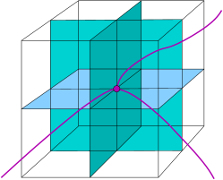
Figure 6: An elementary cell in the Riemann sum (4.29), together with the three surfaces on which the fluxes are evaluated.

Having constructed a sequence of refinements with the correct classical limit, we can now attempt to promote (4.28) to a quantum operator by invoking the known action of each factor $\hat{F}^{a}_{S^{a}_{I}}$ on a spin network wave function, viz.

$$\hat{V}(\Omega)=\lim_{N\rightarrow\infty}\sum_{I=1}^{N}\hat{V}(\Omega_{I})=\lim_{N\rightarrow\infty}\sum_{I=1}^{N}\sqrt{\big{|}\hat{q}_{I}^{(N)}(S^{1}_{I},S^{2}_{I},S^{3}_{I})\big{|}}\,,$$ (4.29)

with the operator (= square of the local volume)

$$\hat{q}_{I}^{{(N)}}(S^{1}_{I},S^{2}_{I},S^{3}_{I}):=\frac{1}{3!}\epsilon_{abc}\hat{F}^{a}_{S^{1}_{I}}[\tilde{E}]\,\hat{F}^{b}_{S^{2}_{I}}[\tilde{E}]\,\hat{F}^{c}_{S^{3}_{I}}[\tilde{E}]\,.$$ (4.30)

Ignoring the square root for the moment, (4.30) is indeed well defined as an operator at this point. However, unlike the classical volume, the action of $\hat{q}_{I}^{{(N)}}$ on the spin network wave function depends on the way we partition $\Omega$, and more specifically on the position of the faces $S^{a}_{I}$ in relation to the edges and vertices. As a simple example of the inherent ambiguities consider a cube which is traversed by one edge $e$, but not containing any vertex of the network. If the surfaces $S^{a}_{I}$ are positioned in such a way that the edge intersects each one of them with ${\iota}(e,S^{a}_{I})\neq 0$ at three different points in $\Omega_{I}$, the operator simply inserts the matrices $\tau^{1},\tau^{2}$ and $\tau^{3}$ at the appropriate places in $h_{e}[A]$. If the cell is sufficiently small, we can bring these matrices together, using $\tau^{1}\tau^{2}\tau^{3}=i$, and thus pick up a contribution of order one. It is easy to construct sequences of refinements such that an arbitrarily large number of cells $\Omega_{I}$ gives such a contribution, no matter how small the cells are. In order to prevent catastrophic divergent sums from appearing on the r.h.s. of (4.29) one must therefore rule out such configurations ‘by hand’ and stipulate that each cell $\Omega_{I}$ may contain at most two such intersections with any edge, in which case one of the three factors in (4.30) will give zero.

With this proviso, the sum receives contributions only from those cells $\Omega_{I}$ which contain a vertex $v$. If the vertex $v$ does not coincide with the intersection point of the three faces $S_{I}^{a}$, further refinement will yield more cells, which do not contribute by the above requirement. Hence, with sufficient refinement only those cells will remain and contribute for which the vertex $v$ sits precisely at the intersection: $v=S^{1}_{I}\cap S^{2}_{I}\cap S^{3}_{I}$. This means that we must also exclude refinements such as in figure 7 for which $S^{1}_{I}\cap S^{2}_{I}\cap S^{3}_{I}$ ‘misses’ $v$ by an amount that gets smaller with $N$, but never vanishes for $N<\infty$.

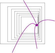
Figure 7: A series of refining steps for one cell in a Riemann sum, such that the indicated node is never at the centre of any of the boxes except in the strict $N\rightarrow\infty$ limit. A volume operator based on cells of this kind would always yield a vanishing result for any finite cell size.

With these assumptions, the resulting action of the operator $\hat{q}_{I}$ on the vertex $v$ reduces to

$$\hat{q}_{I}=(8\pi l_{P}^{2}\gamma)^{3}\frac{1}{48}\sum_{e_{1},e_{2},e_{3}}\epsilon(e_{1},e_{2},e_{3})\epsilon_{abc}\hat{J}_{a}^{(e_{1})}\hat{J}_{b}^{(e_{2})}\hat{J}_{c}^{(e_{3})}\,,$$ (4.31)

where the sum runs over all possible triplets of edges in the vertex $v$, and the angular momentum operator $\hat{J}^{(e,v)}_{a}$ (defined in (4.17)) by definition inserts a matrix $\rho_{j_{e}}(\tau^{a})$ at the vertex $v$ into the spin network wave function. The coefficients $\epsilon(e_{1},e_{2},e_{3})$ are orientation factors which are equal to $\pm 1$. They depend on how the faces $S^{a}_{I}$ cut across the vertex, and on which edges are ‘above’ and ‘below’ $S^{a}_{I}$. More precisely, in terms of the factors $\sigma(e,S)$ introduced in (4.17) they are given by

$$\epsilon(e_{1},e_{2},e_{3})=\sigma(e_{1},S^{1}_{I})\,\sigma(e_{2},S^{2}_{I})\,\sigma(e_{3},S^{3}_{I})$$ (4.32)

and thus completely fixed by the relative positions of the edges and the surfaces. Let us also stress they are independent of any fiducial metric background structure, and purely combinatorial – hence invariant under diffeomorphisms. (4.32) is not yet the final answer, but let us first make the above formulas a little more concrete by working out the action of the above operator on a 4-valent vertex (4.5). Its net effect is the replacement of the intertwiner according to

$$C_{\alpha_{1}\ldots\alpha_{4}}^{j_{1}\ldots j_{4}}\rightarrow\text{const}.\!\!\!\!\!\!\!\sum_{\text{perm.}\{1,2,3,4\}}\;\epsilon(e_{1},e_{2},e_{3})\;\epsilon_{abc}\\[-2.15277pt] \times\Big{(}\rho_{j_{e_{1}}}(\tau^{a})\Big{)}_{\alpha_{1}\beta_{1}}\,\,\Big{(}\rho_{j_{e_{2}}}(\tau^{b})\Big{)}_{\alpha_{2}\beta_{2}}\,\,\Big{(}\rho_{j_{e_{3}}}(\tau^{c})\Big{)}_{\alpha_{3}\beta_{3}}\,\,\delta_{\alpha_{4}\beta_{4}}C^{j_{e_{1}}\ldots j_{e_{4}}}_{\beta_{1}\ldots\beta_{4}}\,,$$ (4.33)

where the sum runs over all choices of three edges out of four. From this formula it is obvious that in general the operator $\hat{q}_{I}$ acts non-diagonally on a spin network wave function $|\Gamma,\{j\},\{C\}\rangle$, because it changes the intertwiners $\{C\}$, although it does not affect the spin network itself (i.e. the graph $\Gamma$). The operator vanishes when all the edges enter $v$ through the same octant, in which case $\epsilon=+1$ for all choices, and

$$\epsilon_{abc}\big{(}\hat{J}_{1}^{a}\hat{J}_{2}^{b}\hat{J}_{3}^{c}+\hat{J}_{1}^{a}\hat{J}_{2}^{b}\hat{J}_{4}^{c}+\hat{J}_{1}^{a}\hat{J}_{3}^{b}\hat{J}_{4}^{c}+\hat{J}_{2}^{a}\hat{J}_{3}^{b}\hat{J}_{4}^{c}\big{)}=0$$ (4.34)

by angular momentum conservation, $\hat{J}_{1}^{a}+\hat{J}_{2}^{a}+\hat{J}_{3}^{a}+\hat{J}_{4}^{a}=0$. Note that we can in principle arrange any 4-valent vertex to conform with this choice (see figure 8). Similar results hold true when yet more edges enter the vertex from one octant.

\psfrag{OR }{or}\includegraphics*[height=113.81102pt]{ambiguity2.eps}

Figure 8: Two different choices for the relative orientation of the edges emanating from a four-valent node and the cell used in the definition of the volume operator (prior to averaging over the positions of the surfaces $S_{I}$). It is always possible to choose the division of the cell such that all four edges emanate from the same octant. We have here drawn the ‘active’ version in which the edges rather than the surfaces are deformed. Note that these two configurations are not homotopically related.

Let us now return to the coefficients $\epsilon(e_{1},e_{2},e_{3})$ in (4.32). Though manifestly background independent they do depend on how we choose to position the faces and edges: for instance, there is no a priori argument that would force a given edge linking two vertices in adjacent cells to appear ‘to the left’ or ‘to the right’ of the face connecting the two vertices, as illustrated in figure 9, and in fact almost any combination of factors $\pm 1$ is possible. To eliminate this remaining ambiguity in the definition of the volume operator, one now averages over the various possibilities . More specifically, this is done by integrating over the positions of the surfaces with some measure ${\rm d}\mu(\theta_{1},\theta_{2},\theta_{3})$, where the $\theta_{i}$ are suitable angular coordinates, viz.

$$\hat{\epsilon}(e_{1},e_{2},e_{3}):=\int{\rm d}\mu(\theta_{1},\theta_{2},\theta_{3})\;\sigma(e_{1},S^{1}_{I}(\theta_{1}))\,\sigma(e_{2},S^{2}_{I}(\theta_{2}))\,\sigma(e_{3},S^{3}_{I}(\theta_{3}))\,.$$ (4.35)

\psfrag{OR }{or}\includegraphics*[height=113.81102pt]{ambiguity1.eps}

Figure 9: Sign ambiguities in the volume operator, present because the relative location of the three surfaces $S_{I}$ and the edges of the spin network can be chosen in different ways (again prior to averaging, as in figure 8).

This leads to a well defined combinatorial answer depending on the relative orientation of the three edges $(e_{1},e_{2},e_{3})$ (= the sign of the determinant of the dreibein spanned by the tangents to the three edges at the vertex), but only modulo an overall factor which encapsulates the freedom in the choice of the measure ${\rm d}\mu$. In principle such a factor can arise for each vertex, but in order to preserve diffeomorphism invariance of the volume these factors should be chosen to be the same for all vertices. This factor is the one ambiguity which remains in the definition of the volume operator, and this ambiguity cannot be eliminated [109].

Finally, given an assignment of $\hat{\epsilon}(e_{1},e_{2},e_{3})$ for each vertex, how do we actually compute the spectrum of the volume operator in (4.29)? First of all, it is easy to see that this operator always vanishes on three-valent vertices which satisfy the Gauss constraint. This is a direct consequence of angular momentum conservation, or equivalently

$$\epsilon_{abc}\Big{(}\rho_{j_{e_{1}}}(\tau^{a})\Big{)}_{\alpha_{1}\beta_{1}}\Big{(}\rho_{j_{e_{2}}}(\tau^{b})\Big{)}_{\alpha_{2}\beta_{2}}\Big{(}\rho_{j_{e_{3}}}(\tau^{c})\Big{)}_{\alpha_{3}\beta_{3}}\,C^{j_{e_{1}}\,j_{e_{2}}\,j_{e_{3}}}_{\beta_{1}\beta_{2}\beta_{3}}=0\,.$$ (4.36)

In other words, the volume operator vanishes on gauge invariant two- and three-valent vertices (but not on gauge variant ones), and picks up contributions only from spin networks with vertices of valence $\geq 4$. Given any spin network wave function, the first step is to work out the action of $\hat{q}_{I}$ according to the above rules. In a second step this action must be diagonalised for each $I$ on the spin network wave functions. This can be done because the operators $\hat{q}_{I}$ commute amongst each other, i.e. $[\hat{q}_{I},\hat{q}_{I^{\prime}}]=0$ for $I\neq I^{\prime}$. Only now can we define the absolute value $|\hat{q}_{I}|$ and take the square root $\sqrt{|\hat{q}_{I}|}$ using the spectral decomposition of this operator (note that $\hat{q}_{I}$ is not necessarily a positive operator). Unfortunately, these steps are all but straightforward to carry out in practice [116]. The analysis can be simplified by applying the operator identity [115, 117]

$$\epsilon_{abc}J^{1}_{a}J^{2}_{b}J^{3}_{c}=\frac{i}{4}\big{[}({\bf J}^{1}+{\bf J}^{2})^{2},({\bf J}^{2}+{\bf J}^{3})^{2}\big{]}$$ (4.37)

to any three edges entering the vertex, enabling a numerical analysis of simple configurations with low-valence nodes. This procedure has recently been used to show that the operator corresponding to the inverse volume is not bounded from above when acting on zero-volume spin network states [41] (in marked contrast to the symmetry reduced models of [38], where the avoidance of an initial singularity hinges on the fact that the operator corresponding to the ‘inverse volume’ is bounded from above). Nevertheless, the resulting formulas remain very complicated. The lack of a more explicit representation for the operators $\sqrt{\hat{q}_{I}}$ is also a serious impediment towards a better understanding of the Hamiltonian constraint.

4.5 Some comments on regularisation dependence

At this point some comments regarding the regularisation procedures for kinematical operators which we have outlined above, are in order. Similar comments will apply to the regularisation of the Hamiltonian constraint operator. First of all it should be evident from the foregoing discussion that the notions of ‘finiteness’ and ‘regulator independence’ as currently used in LQG are not the same as in conventional quantum field theory. There one insists that renormalised quantities should come out the same (modulo a finite number of normalisations) after removal of the regulator, no matter how the latter is chosen. By contrast, LQG does not claim that different prescriptions for constructing an operator will always lead to the same physical result. This is well illustrated by the volume operator, whose definition and whose very existence hinge on various choices that have been made along the way.

Let us nevertheless briefly summarise what is meant here by ‘regularisation’. In order to regulate a given classical phase space quantity defined by an integral (such as the volume), one first approximates that integral by a Riemann sum (which is of course assumed in the classical theory to converge to the desired quantity in the limit of infinite refinement). One then replaces in this finite Riemann sum all terms by operators, usually in such a way that the various area or volume elements are absorbed into the definition of these operators (as exemplified by the ‘small’ operators $\hat{F}^{a}_{S^{a}_{I}}[\tilde{E}]$ entering the definition of the area and volume operators). Acting with a sequence of these discretised operators on an arbitrary, but fixed spin network state, the resulting sequence of refinements (labelled by $N$, say) eventually becomes stationary (i.e. constant for $N$ sufficiently large), because the state is kept fixed as the limit $N\rightarrow\infty$ is taken. This follows straightforwardly for the area operator, but requires a choice of ‘preferred’ regularisations for the volume operator. With these choices, the ‘correct’ result is always obtained already after a finite number of refinements. A good analogy would be the Riemann integral of a step function, for which a suitably refined Riemann sum attains the exact value already after finitely many steps, after which the result no longer depends on the ‘regulator’ (i.e. the size of the intervals defining the Riemann sum). In this sense, the results of LQG are indeed ‘regulator independent’.

From what has just been said, it is evident that infinities can never appear in the LQG regularisation procedure, and in this sense the resulting theory is ‘finite’, at least as far as the kinematical operators are concerned. LQG nevertheless requires the regularisation of the area and volume operators in order even to be able to define the quantum counterparts of the classical constraints via Thiemann’s trick. The outlined regularisation is, therefore, not introduced to remove divergences. Standard short distance, QFT divergences ‘disappear’ in the LQG approach by the very construction of the theory: all states are discrete, and at any step of the calculation one deals only with a finite number of objects. The price one pays are ambiguities of the type encountered above, some of which can only be eliminated by making ad hoc choices, such as the rule prescribing the way in which an edge has to traverse a cell. We shall encounter more such ambiguities when we attempt to define the Hamiltonian constraint operator.

Of course, these considerations do not necessarily imply any inconsistency. Namely, one can always adopt the above prescriptions for the kinematic operators as definitions, which can be plausibly related to the corresponding classical objects, and in this sense the definitions of the above operators in LQG are perfectly acceptable. What we would like to emphasise, however, is that with this construction the work is hardly begun. The far more difficult task is now to show that these definitions, when put together and inserted in the constraints, yield a sensible quantum theory, and a consistent quantum constraint algebra, in particular. The situation here is reminiscent of the one in the early days of constructive quantum field theory (see e.g. [118] and references therein). The problem then was not so much finding non-perturbative regulators and establishing the existence of selected limits when the regulator is removed. Rather, the main problem was to establish that the resulting theory has all the desired physical properties, to wit, full Poincaré invariance, locality and causality. As is well known, no interacting quantum field theory in four dimensions satisfying all these requirements is known to this day . And for those low dimensional models which could actually be shown to exist and possess all the requisite properties, the tightly knit construction left no room for ambiguities other than the normalisation of a finite number of physical parameters (masses and coupling constants).

4.6 Coupling to matter fields

Any realistic theory of quantum gravity should at least allow for a coupling to the matter fields of the Standard Model of elementary particles. In the framework of geometrodynamics it is fairly easy to extend the relevant formulas to incorporate matter fields (but, of course, the difficulties with quantisation remain the same as before). Likewise, it is possible to include gauge fields and fermions in the LQG formalism, essentially without any restriction on the gauge group or the number and structure of fermion families — as we already pointed out LQG does not appear to put any restrictions on the matter couplings (such as renormalisability). Armed with the translation rules of section 3.2, the transition from the ‘old’ metric or dreibein variables to the loop variables is in principle straightforward, though usually cumbersome (and, we may add, of considerably diminished esthetical appeal in comparison with Ashtekar’s original reformulation of pure gravity). Because there is an ample literature on this subject (see e.g. [119, 120, 121, 122, 123, 124]), and because the introduction of matter couplings does not alleviate the problems with the Hamiltonian constraint in LQG, we will be very brief and only mention two selected aspects here.

Consider, for example, the coupling of fermion fields in the LQG setting [119, 125]. The starting point is the classical continuum action of a Dirac fermion coupled to gravity

$$S=\int\!{\rm d^{4}}x\,E\,\bar{\chi}\gamma^{A}E_{A}{}^{\mu}{\cal D}_{\mu}\chi\equiv\int\!{\rm d^{4}}x\,E\,\bar{\chi}\gamma^{A}E_{A}{}^{\mu}\big{(}\partial_{\mu}+\omega_{\mu BC}\gamma^{BC}\big{)}\chi\,,$$ (4.38)

where we have omitted a possible mass term for simplicity, as its inclusion would pose no new conceptual problems. There are two immediate questions one faces when trying to construct quantum Hamiltonian for this system. One is the choice of the conjugate pair of variables for fermions; finding the proper fermionic variables may also require redefinitions of the other fields so as to ‘diagonalise’ the canonical (Poisson or Dirac) brackets. For instance, for the above model it turns out [120] that a good choice for the conjugate pair of fermionic variables is the pair of half-densitised spinors

$$\tilde{\chi}\equiv\sqrt[4]{\det\tilde{E}}\,\psi\,,\quad\pi=i{\tilde{\chi}}^{\dagger}\gamma^{0}\,.$$ (4.39)

If instead of densitised spinors we used bare spinors (without any factors of the determinant of the dreibein), one would have to modify the gravitational connection [120] in order to obtain diagonal canonical brackets, but at the expense of making the connection complex again

$$\tilde{A}_{m}^{a}=-\frac{1}{2}\epsilon^{abc}\omega_{m\,bc}+\gamma K_{m}^{a}+\frac{i}{4\sqrt{\tilde{E}}}e_{m}^{a}\bar{\chi}\chi\,.$$ (4.40)

This leads to a new reality problem, similar to the one already encountered in [76], and not different from the one which eventually led LQG to abandon the ‘old’ Ashtekar variables with $\gamma=\pm i$. The second question is how to express all variables in terms of the LQG variables $h_{e}[A]$ and $F^{a}_{S}[\tilde{E}]$. The answer to this question can be obtained by employing the identities (3.26) and (3.27). A similar procedure will be spelled out in the next section in order to construct the Hamiltonian constraint, so we will refrain here from giving more details.

When implementing the matter Hamiltonians in terms of spin networks, the description of (abelian or non-abelian) gauge fields and matter fields is somewhat similar to the description of standard lattice gauge theories: matter fields (scalars or fermions) are attached to the vertices of the spin network, while gauge fields are associated to the edges (links), see e.g. [121, 122, 123] for a treatment of electromagnetism and [124] for scalar field theories in the LQG formalism. There are, however, two main differences between lattice gauge theory and LQG. In the former, the space or spacetime lattice is given, and hence there are only three (or four) possible directions for the edges. The coupling between two fermions $\chi_{1}$ and $\chi_{2}$ on adjacent vertices 1 and 2 connected by an edge $e\equiv(12)$, is uniquely given by $\bar{\chi}_{1}\gamma_{12}h_{12}[A]\chi_{2}$, where $\gamma_{12}$ is the $\gamma$-matrix ‘along’ the edge (12). In LQG (and in general relativity), this simple formula fails because the direction of the link is arbitrary, and a vielbein factor must be inserted to ‘align’ the $\gamma$-matrix with the holonomy. When rewriting the dreibein by means of the formulas of section 3.2, this usually leads to rather awkward expressions in terms of the spin network variables $h_{e}[A]$ and $F^{a}_{S}[\tilde{E}]$. This problem is further compounded by a second difficulty which goes back to the issue of what the correct value is for the Barbero-Immirzi parameter. As we mentioned already, for $\gamma\neq\pm i$, the connection $A$ is not the pullback of the (chiral) spin connection. Therefore, the holonomy $h_{12}[A]$ does not effect the correct parallel transport between $\chi_{1}$ and $\chi_{2}$, and must accordingly be amended by further (and again rather awkward) modifications.

We should stress that, even when one has obtained an expression for the matter action in terms of spin network operators, one does not know whether the resulting quantum theory has any relation to the usual Fock-space quantised theory. Showing that such a relation exist requires the field-theory analogues of the ‘shadow states’ for point particles [18]. These states are complicated linear combinations of elementary spin network states, approximating Fock space coherent states. In flat space some results have been obtained in the case of Maxwell [121, 122, 123] and scalar fields [124]. Recent attempts to construct coherent states in the presence of gravity include [19, 20, 21, 22, 23, 24, 101, 102].

A completely different question concerns the role of the structure group SU(2), and the possibility of generalising Ashtekar’s variables to higher dimensions, to achieve a Kaluza-Klein type unification of matter and gravity. The closure of the classical constraint algebra in the Ashtekar reformulation of gravity requires use of the identity $\epsilon_{abe}\epsilon^{cde}=2\delta^{cd}_{ab}$, which is only valid for the structure constants of the group SU(2) and its non-compact form SO(1,2). These properties no longer hold for SU($N$) when $N>2$. For this reason, the LQG reformulation of gravity works only in three and four spacetime dimensions. Nevertheless, one can try to generalise the formalism to SU($N$) [126] and thereby arrive at a novel type of coupling between gravity and Yang-Mills fields [127, 128]. A very different attempt to generalise the formalism to include matter couplings is based on the observation that an inverse densitised vielbein also appears naturally in certain reformulations of $D=11$ supergravity [129]. It is not known whether any of these ansätze can be implemented in a spin network formulation (although replacing SU(2) holonomies by SU($N$) holonomies seems straightforward enough).

5 Quantum constraints

As we have seen in section 3.1, the Hamiltonian framework leads to three classical constraints: the Gauss, diffeomorphism and Hamiltonian constraints. To implement these constraints at the quantum level, one must first properly define them, i.e. express them in terms of the elementary variables, the holonomies and fluxes, and then investigate their properties. We will first discuss the kinematical constraints, which are ‘easy’ (relatively speaking), whence we can be brief. We will then turn to the truly difficult part of the story – the Hamiltonian constraint.

5.1 Kinematical constraints

The Gauss constraint is already expressed in canonical variables $h_{e}[A]$ and $F_{S}[\tilde{E},f]$, and one can solve it exactly. This is simply because fulfilment of the Gauss constraint is equivalent to the gauge invariance of the spin network wave function: invariance is simply achieved by contracting the SU(2) representation indices entering a given vertex in an SU(2) invariant manner. Equivalently, one says that angular momentum is conserved at each vertex, viz.

$$\sum_{e}\hat{J}_{(e,v)}^{a}=0$$ (5.1)

for each $v\in\Gamma$. Recall (see the discussion around (4.17)) that the operator $\hat{J}^{(e,v)}_{a}$ is defined to act by inserting a matrix $\rho_{j_{e}}(\tau^{a})$ at the vertex $v$ in the representation belonging to the (oriented) edge $e$, with appropriately contracted SU(2) representation indices, and appropriate orientation. For the following discussion, we will tacitly assume that the wave function satisfies the Gauss constraint, whenever appropriate.

The diffeomorphism constraint is more difficult to impose — unlike in geometrodynamics, one cannot immediately write down formal expressions which are manifestly diffeomorphism invariant, because the spin network functions are not supported on all of $\Sigma$, but only on one-dimensional links. Nevertheless, it would seem most natural at first sight to try to solve the diffeomorphism constraint on the kinematical Hilbert space ${\cal H}_{\rm kin}$. However, this is impossible for two reasons. First of all, the diffeomorphism generator does not even exist as an operator: there is no way to differentiate finite diffeomorphisms so as to obtain ‘infinitesimal’ ones due to the lack of weak continuity (and a fortiori, differentiability). Secondly, with the exception of the trivial state $\Psi={\bf 1}$ (the empty spin network), there is just no diffeomorphism invariant state in ${\cal H}_{\rm kin}$. This is intuitively clear because every spin network state changes under a diffeomorphism which moves the associated graph around. For these reasons, LQG invokes a variant of the so-called ‘group averaging’ method, but in a way that is different from the standard group averaging procedure. Namely, application of the latter would require knowing an integration measure ${\rm d}\mu(\phi)$ on the infinite dimensional group Diff$(\Sigma)$. The formally diffeomorphism invariant state would then be

$$\Psi^{\text{inv}}_{\Gamma,\psi}[A]\stackrel{{\scriptstyle?}}{{=}}\int_{\text{Diff}(\Sigma)}{\rm d}\mu(\phi)\,\Psi_{\Gamma,\psi}[A\circ\phi]\,,$$ (5.2)

and if the measure existed, this state would legitimately belong to ${\cal H}_{\rm kin}$. For the infinite dimensional group Diff$(\Sigma)$ no such measure is known (the ‘counting measure’ (5.6) introduced below does not ‘live’ on ${\cal H}_{\rm kin}$, but leads out of the kinematical Hilbert space), hence the above expression is devoid of meaning — confirming the conclusion above that ${\cal H}_{\rm kin}$ does not admit non-trivial solutions. LQG circumvents this difficulty by implementing ‘group averaging’ in a way that is more adapted to the non-separable Hilbert space and the properties of the scalar product (4.7). The key observation here is that the constraint can be formally solved on a much larger space, namely the algebraic dual ${\cal D}^{*}$ of some dense subspace ${\cal D}$ of ${\cal H}_{\rm kin}$, such that

$${\cal D}\subset{\cal H}_{\rm kin}\subset{\cal D}^{*}\,.$$ (5.3)

Typically, the dual space ${\cal D}^{*}$ is thus a space of distributions. This is not as outlandish as it may seem at first, because for constrained systems, the solutions of the constraints are generically distributions, see e.g. [130] . Given any (densely defined and closable) operator ${\cal O}$ and its adjoint ${\cal O}^{\dagger}$ with domain ${\cal D}\subset{\cal H}_{\rm kin}$, the action of the dual operator ${\cal O}^{*}$ on the algebraic dual ${\cal D}^{*}$ of ${\cal D}$ is defined for any particular element ${\cal X}\in{\cal D}^{*}$ by requiring

$$\langle{\cal O}^{*}{\cal X}\,|\,\Psi\rangle=\langle{\cal X}\,|\,{\cal O}^{\dagger}\Psi\rangle$$ (5.4)

to hold for all $\Psi\in{\cal D}$. The space ${\cal D}^{*}$ is very large, and in practice one restricts attention to a physically motivated vector subspace thereof, the so-called ‘habitat’ ${\cal V}^{*}\subset{\cal D}^{*}$, whose specification is closely related to the definition of the Hamiltonian constraint. Observe also that the above definition does not require the operator ${\cal O}$ to be hermitean.

The obvious (‘canonical’) choice for ${\cal D}$ is

$${\cal D}={\cal S}$$ (5.5)

that is, the space of finite linear combinations of spin network states. However, there may exist other viable choices for ${\cal D}$. The dual space ${\cal S}^{*}$ is much larger than ${\cal H}_{\rm kin}$, and actually too large for our purposes. What is important here is that ${\cal S}^{*}$ contains a certain subspace of diffeomorphism invariant states, and its completion w.r.t. to the norm (5.8) below. This subspace is contained in any of the proposed ‘habitats’ ${\cal V}^{*}$, and is obtained by averaging spin network states. More specifically, for any $\Psi_{\Gamma}\in{\cal S}$ associated with a particular graph $\Gamma$ we define the ‘group average’ by the formal sum

$$\eta(\Psi_{\Gamma})\equiv\overline{\Psi}_{\Gamma}:=\sum_{\phi\in{\rm Diff}(\Sigma|\Gamma)}\phi^{*}\circ\Psi_{\Gamma}$$ (5.6)

where $(\phi^{*}\circ\Psi)[A]:=\Psi[A\circ\phi]$, and where Diff$(\Sigma|\Gamma)$ consists of the subgroup of Diff$(\Sigma)$ obtained by dividing out the diffeomorphisms leaving invariant the graph $\Gamma$ on which $\Psi_{\Gamma}$ lives. While $\Psi_{\Gamma}\in{\cal S}$ by assumption, averaging the state in this way throws it out of ${\cal S}$ and also ${\cal H}_{\rm kin}$. At first sight, this seems to make matters worse: we have replaced the ill-defined integral over Diff$(\Sigma)$ by a highly formal continuous sum. However, the day is now saved by two facts: $(i)$ unlike the integral, the sum no longer requires unavailable detailed knowledge of the properties of Diff$(\Sigma)$, and $(ii)$ when applying an averaged spin network state $\eta(\Psi_{\Gamma^{\prime}})$ (considered as a bra-vector) to any other spin network state $\Psi_{\Gamma}[A]$, the sum

$$\langle\eta(\Psi_{\Gamma^{\prime}})\,|\,\Psi_{\Gamma}\rangle=\sum_{\phi\in{\rm Diff}(\Sigma|\Gamma^{\prime})}\langle\phi^{*}\circ\Psi_{\Gamma^{\prime}}\,|\,\Psi_{\Gamma}\rangle$$ (5.7)

consists at most of a finite number of terms, and it is this fact which ensures that $\eta(\Psi_{\Gamma})$ is indeed well defined as an element of the dual space ${\cal S}^{*}$. Namely, there is no contribution at all if $\Gamma$ and $\Gamma^{\prime}$ are not diffeomorphic. For $\Gamma$ and $\Gamma^{\prime}$ diffeomorphic, only that term contributes for which $\Gamma$ and $\phi^{*}\circ\Gamma^{\prime}$ coincide. In the above equation, the bracket on the r.h.s. is just the scalar product (4.7), while the bracket on the l.h.s. denotes the dual pairing between ${\cal S}$ and ${\cal S}^{*}$.

We can now promote the space of averaged diffeomorphism invariant spin network states to a pre-Hilbert space by ‘dividing out the volume of the gauge group’ ( = Diff($\Sigma$)). More precisely, we define the scalar product between two such states as

$$\langle\!\langle\eta(\Psi_{\Gamma^{\prime},\psi^{\prime}})\,\big{|}\,\eta(\Psi_{\Gamma,\psi})\rangle\!\rangle:=\langle\eta(\Psi_{\Gamma^{\prime},\psi})\,\big{|}\,\Psi_{\Gamma,\psi}\rangle\,.$$ (5.8)

Here the bracket on the r.h.s. is the dual pairing between ${\cal S}$ and ${\cal S}^{*}$, and the bracket $\langle\!\langle.|.\rangle\!\rangle$ on the l.h.s. denotes the new scalar product. The new Hilbert space ${\cal H}_{\rm diff}$ of diffeomorphism averaged states is then obtained by completion w.r.t. this norm, and can be thought of to consist of the averaged versions of the states (4.8) (but let us emphasise again that it is not a subspace of ${\cal H}_{\rm kin}$). Observe that the Hilbert space ${\cal H}_{\rm diff}$ is still a ‘small’ subspace of ${\cal S}^{*}$ because the vast majority of elements in ${\cal S}^{*}$ does not correspond to diffeomorphism averaged spin network states, and cannot be obtained as limits of such states w.r.t. to the above norm. Moreover, ${\cal H}_{\rm diff}$ is ‘smaller’ than the original kinematical Hilbert space ${\cal H}_{\rm kin}$, because distinct elements of the latter which are related by a diffeomorphism get mapped to the same element of ${\cal S}^{*}$; equivalently, the averaging map has a very large kernel. There is no way to extend the above norm from ${\cal H}_{\rm diff}$ to all of ${\cal S}^{*}$, in accordance with the fact that distribution spaces cannot be made into Hilbert spaces, but at best into topological vector spaces; however, there appears to be no consensus as to which of the many possible topologies is the right one for ${\cal S}^{*}$. While ${\cal H}_{\rm kin}$ is non-separable, it is expected that ${\cal H}_{\rm diff}$ is separable [134, 135] provided one averages over homeomorphisms rather than diffeomorphisms (if one divides out only by analytic or $C^{\infty}$ diffeomorphisms, ${\cal H}_{\rm diff}$ remains non-separable, see also [12] for a recent discussion of this point).

Which, then, is the arena, or ‘habitat’, in which quantum gravity takes place according to LQG, and where one must ultimately consider the action of the Hamiltonian constraint? The foregoing discussion shows that there is no easy answer to this question, and apparently also no complete consensus in the community as to which space is ‘right’. The Hilbert space ${\cal H}_{\rm diff}$ of diffeomorphism averaged states certainly appears to be a good starting point for implementing and solving the Hamiltonian constraint, but it may not be good enough. The reason is that the action of the Hamiltonian constraint in general does not preserve ${\cal H}_{\rm diff}$; in other words, it maps diffeomorphism invariant states into ones that are not invariant. Consequently, when checking the commutator of two Hamiltonian constraints, one must again pass to a larger space, which is preserved by the action of the Hamiltonian, but which is no longer a Hilbert space. An explicit example are the ‘vertex-smooth’ states introduced in [29], obeying $\langle{\cal X}|\Psi_{1}\rangle=\langle{\cal X}|\Psi_{2}\rangle$ for all $\Psi_{1},\Psi_{2}$ which are related by a diffeomorphism that leaves the vertices of the spin network fixed. Alternatively, it has been proposed to implement the Hamiltonian constraint on the kinematical Hilbert space ${\cal H}_{\rm kin}$ via a weak $\!{}^{*}\!$ limit [27], see also the following section. At any rate, the challenge here — as with any other constrained quantum mechanical system — is to find a subspace that is annihilated by all the constraints, and to define a physical inner product which yields the ‘final’ physical Hilbert space.

5.2 Hamiltonian constraint

As we explained, the diffeomorphism constraint is imposed not in terms of an operator constraint, but through the formal group averaging method. By contrast, the Hamiltonian constraint is imposed as an operator constraint. Hence, as a zeroth step, one has to construct this Hamiltonian operator. As we explain in more detail below, in this derivation one is forced, at a certain stage, to make choices concerning the action of the Hamiltonian operator on a generic spin network state. Thus the resulting definition is indeed motivated by the classical expression for the Hamiltonian (expressed in loop variables), but it is plagued by a very large number of ambiguities . To test the proposed prescription and compare it with other possibilities, one would need to find states which are annihilated by the Hamiltonian, and check that in the semi-classical limit these states produce sensible results. This is, however, currently out of reach: due to the great complexity of the proposed Hamiltonian, not a single physically interpretable eigenstate is known. While this should not come as a surprise (after all, we have no reason to expect to be able to solve the theory exactly), it is remarkable that even the far more modest goal of working out in complete detail the action of the (regulated) Hamiltonian on a general spin network wave function appears difficult to attain.

Even if we can work out the action of the Hamiltonian on any given element of ${\cal S}$, we are not done. As explained in the previous subsection, in order to ensure satisfaction of the diffeomorphism constraint, we must transfer the action of the Hamiltonian to the dual space ${\cal S}^{*}$, or at least to some physically motivated subspace ${\cal V}^{*}$ thereof. Below, we will be mostly dealing with a regulated Hamiltonian $\hat{H}[N,\epsilon]$ (where $N$ is the lapse function). Here, the regularisation parameter $\epsilon>0$ enters via a plaquette $P(\epsilon)$, which is attached to a vertex and which must be shrunk to zero at the end of the calculation. However, for a given $\Psi$, the limit $\epsilon\rightarrow 0$ of $\hat{H}[N,\epsilon]\Psi$ does not exist on ${\cal S}$, because wave functionals supported on the same network, but with an extra loop $\partial P(\epsilon)$ attached to one of the vertices, are orthogonal to one another for different values of $\epsilon$ by (4.7). For this reason, one must resort to a weaker notion of limit by transferring the action of the Hamiltonian to the dual space. More specifically, we define the limit $\epsilon\rightarrow 0$ by demanding

$$\langle\hat{H}^{*}[N]{\cal X}\,|\,\Psi\rangle=\lim_{\epsilon\rightarrow 0}\;\langle{\cal X}\,|\,\hat{H}[N,\epsilon]\Psi\rangle$$ (5.9)

to hold for all $\Psi\in{\cal S}$ and ${\cal X}\in{\cal V}^{*}$. Here ${\cal V}^{*}\subset{\cal S}^{*}$ is the ‘habitat’ already mentioned in the previous subsection, a vector subspace of ${\cal S}^{*}$. The choice of ${{\cal V}}^{*}$ should be physically motivated. Natural choices are ${\cal V}^{*}={\cal H}_{\rm diff}$ or the space of vertex smooth states [29], but there may be others. An evident requirement here is, of course, that the choice of ${\cal V}^{*}\subset{\cal S}^{*}$ should be such that the limit (5.9) exists. Although it is not entirely clear (to us) what precisely the conditions on ${\cal V}^{*}$ should be for this limit to exist, and to what extent they would determine ${\hat{H}}^{*}[N]\chi\in{\cal V}^{*}$ uniquely, it seems obvious that the limit (5.9) will not exist if ${\cal V}^{*}$ is ‘much larger’ than ${\cal H}_{\text{diff}}$. There is an alternative point of view, which does not require ‘habitats’: according to [27, 74], the choice ${\cal V}^{*}={\cal H}_{\rm diff}$ in fact is singled out, and formula (5.9) should not be viewed as defining a dual Hamiltonian on ${\cal V}^{*}$, but rather as defining the limiting Hamiltonian as a weak $\!{}^{*}\!$ limit on the kinematical Hilbert space ${\cal H}_{\rm kin}$ w.r.t. the weak $\!{}^{*}\!$ topology defined by ${\cal V}^{*}={\cal H}_{\rm diff}$ . In that interpretation, only the r.h.s. of (5.9) is meaningful — but let us repeat that there is no state in ${\cal H}_{\rm kin}$ that could be interpreted as “$\lim_{\epsilon\rightarrow 0}\hat{H}[N,\epsilon]\Psi$”.

Independently of whether or not one adopts the ‘habitat’ point of view, an essential ingredient in existing constructions is the ‘diffeomorphism covariance’ of the Hamiltonian. This means that by transferring the action of $\hat{H}$ to the space of diffeomorphism invariant states, the existence of the above limit can be ensured by the fact that the habitat ${\cal V}^{*}$ is sensitive only to the diffeomorphism invariant characteristics of the regulator. This is also borne out by the construction of [29] which takes ${\cal V}^{*}$ to be the (larger) space of ‘vertex smooth states’. (But note that from the point of view of the Hamiltonian action, going to the slightly larger habitat of ‘vertex-smooth’ states does not make much of a difference; namely, when acting on a spin network state, the Hamiltonian does not shift nodes around. Hence its action on ${\cal H}_{\rm diff}$ or on the larger habitat of ‘vertex-smooth’ states is essentially the same.) In addition to restricting the choice of ${\cal V}^{*}$, requiring the limit (5.9) to exist eliminates at least some of the ambiguities inherent in the definition of the Hamiltonian.

To sum up, the Hamiltonian $\hat{H}[N]$ can only be defined, via (5.9), as a weak limit. This is reminiscent of the LSZ formalism of ordinary quantum field theory, where one also defines the asymptotic field operators as weak rather than strong limits. It is remarkable that the known constructions make essential use of the diffeomorphism covariance, and thus implicit use of the constraints, already in the very definition of the Hamiltonian. However, for all we can tell, the question as to which ${\cal V}^{*}$ is ‘best’ is not settled. On a more practical note, and independently of the choice of ${\cal V}^{*}$, we note that the concrete evaluation of the limit requires simultaneous knowledge of the action of the original regulated Hamiltonian $\hat{H}[N,\epsilon]$ on all elements of ${\cal S}$. Furthermore, explicit expressions for the dual Hamiltonian $\hat{H}^{*}[N]$ that could be used for any practical application of the formalism are even more difficult to obtain than for the Hamiltonian acting on spin network states, and certainly beyond the scope of our modest efforts in this section. Nevertheless, we should stress once more that the dual Hamiltonian $\hat{H}^{*}$ is our true object of interest, and that all further considerations (constraint algebra, semi-classical states, and so on) should be based on it, rather than on the regulated Hamiltonian acting on ${\cal S}$. With these caveats in mind, let us now proceed.

To motivate the form of the quantum Hamiltonian one starts with the classical expression, written in loop variables. Despite the simplifications brought about by equation (3.21), the Hamiltonian constraint still looks formidable,

$$H[N]=\int_{\Sigma}\!{\rm d}^{3}x\,N\frac{\tilde{E}_{a}^{m}\tilde{E}_{b}^{n}}{\sqrt{\det\tilde{E}}}\Big{(}\epsilon^{abc}F_{mnc}-\frac{1}{2}(1+\gamma^{2})K_{[m}{}^{a}K_{n]}{}^{b}\Big{)}\,.$$ (5.10)

In order to write the constraint in terms of only holonomies and fluxes, one has to eliminate the inverse square root as well as the extrinsic curvature factors. This can be done [74] using the relations (3.26)–(3.28). Inserting these into the Hamiltonian constraint one obtains the expression

$$H[N]=\int_{\Sigma}\!{\rm d}^{3}x\,N\epsilon^{mnp}\operatorname{Tr}\Big{(}F_{mn}\{A_{p},V\}-\frac{1}{2}(1+\gamma^{2})\{A_{m},\bar{K}\}\{A_{n},\bar{K}\}\{A_{p},V\}\Big{)}\,.$$ (5.11)

This expression is the starting point for the construction of the quantum constraint operator.

The next step is to express the Ashtekar connection $A_{m}$ as well as field strength $F_{mn}$ and the extrinsic curvature $\bar{K}$ in terms of holonomies. As in lattice gauge theory, this requires the introduction of a cell structure. In the classical expression one splits the target space into cells of size $\sim\epsilon^{3}$ in coordinate space. In order to express connections and curvatures in terms of holonomies, one now has to choose edges $e_{m}$ within each cell, along which the holonomies are going to be evaluated. Once the edges $e_{m}$ are chosen, one uses that the connection along a line of coordinate distance $\epsilon$ can be approximated by

$${}\left\{\int_{e}A,V\right\} =-h_{e}[A]^{-1}\big{\{}h_{e}[A],V\big{\}}+o(\epsilon)\,,$$ (5.12)

$${}\left\{\int_{e}A,\bar{K}\right\} =-h_{e}[A]^{-1}\big{\{}h_{e}[A],\bar{K}\big{\}}+o(\epsilon)\,.$$

For the field strength one has the standard lattice expression

$$\int_{P(\epsilon)}F[A]=\frac{1}{2}\Big{(}h_{\partial P(\epsilon)}^{-1}[A]-h_{\partial P(\epsilon)}[A]\Big{)}+o(\epsilon^{3})\,,$$ (5.13)

where $P(\epsilon)$ is a two-dimensional infinitesimal plaquette with boundary $\partial P(\epsilon)$, that shrinks to zero as $\epsilon\rightarrow 0$. The extrinsic curvature is expressed using the relation (3.28), in which in one substitutes (5.13). Finally, as for the volume operator, one replaces integrals with Riemann sums over the cells, which we will again label with $\alpha$.

In order to quantise the classical Hamiltonian (5.11) with the above regularisation, we next elevate all classical objects to quantum operators as described in the foregoing sections, and replace the Poisson brackets in (5.11) by quantum commutators. The resulting regulated Hamiltonian then reduces to a sum over the vertices $v_{\alpha}$ of the spin network with lapses $N(v_{\alpha})$

$$\hat{H}[N,\epsilon]=\sum_{\alpha}\,N(v_{\alpha})\,\epsilon^{mnp}\operatorname{Tr}\Big{(}\big{(}h_{\partial{P_{mn}(\epsilon)}}-h_{\partial{P_{mn}(\epsilon)}}^{-1}\big{)}\,h^{-1}_{p}\,\big{[}h_{p},\hat{V}\big{]}\Big{)}\\[4.30554pt] -\frac{1}{2}(1+\gamma^{2})\sum_{\alpha}N(v_{\alpha})\,\epsilon^{mnp}\operatorname{Tr}\Big{(}h^{-1}_{m}\,\big{[}h_{m},\bar{K}\big{]}\,h_{n}^{-1}\,\big{[}h_{n},\bar{K}\big{]}\,h_{p}^{-1}\big{[}h_{p},\hat{V}\big{]}\Big{)}\,,$$ (5.14)

where we have already assumed a specific ordering of the operators. The fact that the regularisation parameter $\epsilon$ drops out ‘miraculously’ from this expression, and the integral (5.11) can be replaced by the sum (5.14), requires the Hamiltonian density to have the correct weight, and would not work with the weight two density (3.21), cf. footnote 6 on page 6. If one does not want to make reference to any particular spin network, the Hamiltonian can also be expressed more abstractly as a continuous sum

$$\hat{H}[N,\epsilon]=\sum_{{\bf x}\in\Sigma}N({\bf x})\hat{H}({\bf x};\epsilon)$$ (5.15)

which, on any given spin network, reduces to a finite sum as in (5.14). In the remainder, we will keep the regularisation parameter $\epsilon>0$ fixed, and not always indicate it explicitly in the formulas below.

A first stumbling block here is the presence of the volume operator $\hat{V}$ in (5.14). Although its square has been expressed in terms of fluxes in section 4.4.2, the spectrum of this operator is only partially known, see, however, [115, 117, 41] for recent progress (recall that $\hat{q}$ is not necessarily positive). The further evaluation of (5.14) on a given spin network wave function would now in particular require a diagonal basis of spin network states, on which we could determine the square root of $|\hat{q}|$ for each node, cf. (4.30). To treat all the relevant terms, this diagonalisation would have to be repeated several times, along the lines of [117], with intermittent application of other operators. Although all the steps required in this calculation are thus clearly laid out, presently available technology does not, as far as we are aware, allow a complete evaluation of $\hat{H}[N,\epsilon]$ on a given, but arbitrary spin network state. For this reason, we will only be able to exploit certain qualitative properties of the volume operator in our analysis of the Hamiltonian constraint below. We will thus adopt a pragmatical approach in the remainder, performing all computations with the local trilinear operator $\hat{q}$ instead of the volume operator itself, and assume that we can divide by the relevant power of the volume at the end (thereby postponing the most difficult part of the calculation) . Accordingly, the arguments in this section should be viewed as no more than a gedanken calculation, and there is no claim that this is the way the calculation should ultimately be done.

Apart from obvious ordering ambiguities, and the difficulties with volume operator just described, the action of the quantum expression (5.14) on a generic spin network state also depends strongly on the choice of the coordinate system on $\Sigma$. To be more precise, the action depends on whether or not the basis vectors (i.e. the directions $m$,$n$ and $p$) are aligned with the spin network edges at a given node. There exists a large number of possibilities for these alignments, which are not diffeomorphically equivalent, and one might thus simply define the action of the Hamiltonian by employing a particular alignment, as LQG does. Some of these possibilities are explicitly listed below. We regard these choices as genuine ambiguities in the quantisation procedure, in the sense that observables quantities may depend on them, if they can be shown to exist at all. This potential prescription dependence, and the abundance of possible outcomes for physical quantities are most difficult to digest from the perspective of conventional quantum field theory, especially because, the result for the corresponding classical quantity does not depend on such choices when the limit $\epsilon\rightarrow 0$ is taken.

To get an idea of the complications, let us consider the action of the first term in the regulated Hamiltonian constraint, which is occasionally called the ‘Euclidean Hamiltonian’ (because with a Euclidean signature and $\gamma=\pm 1$, the bothersome second term in (5.14) would be absent, as it is for $\gamma=\pm i$ with Lorentzian signature). We will act with this operator on a three-valent vertex $v$ in a spin network, for given $\epsilon>0$. The spin network wave function on which we will act is given by

$$\psi=\big{(}h^{j_{1}}_{e_{1}}\big{)}_{\alpha_{1}\beta_{1}}\big{(}h^{j_{2}}_{e_{2}}\big{)}_{\alpha_{2}\beta_{2}}\big{(}h^{j_{3}}_{e_{3}}\big{)}_{\alpha_{3}\beta_{3}}\,C^{j_{1}j_{2}j_{3}}_{\beta_{1}\beta_{2}\beta_{3}}\ldots\,,$$ (5.16)

where the dots denote other parts of the spin network. Since the Hamiltonian acts node by node, we can restrict our attention to this local structure at $v$. Let us also write out all indices on the Hamiltonian operator, restricted to that part which acts at $v$,

$$\hat{H}=\operatorname{sgn}(\hat{q})\,|\hat{q}|^{-1/2}\,\epsilon^{mnp}\,\big{(}F^{j}_{mn}\big{)}_{\lambda_{1}\lambda_{2}}\big{(}h^{j}_{p}\big{)}^{-1}_{\lambda_{2}\lambda_{3}}\left[\hat{q},\,\big{(}h^{j}_{p}\big{)}_{\lambda_{3}\lambda_{1}}\right]+\ldots\,,$$ (5.17)

where the dots now denote terms which act at other vertices. The choice of the spin $j$ is a new ambiguity. In the first step, the operator $h_{p}^{-1}[h_{p},\,{\hat{q}}]={\hat{q}}-h^{-1}_{p}\,{\hat{q}}\,h_{p}$ acts at the vertex of the network. When ${\hat{q}}$ in the second term acts on three holonomies already present in the spin network, the result cancels against the first term. (Note that the result only vanishes because we are using ${\hat{q}}$ instead of $\hat{V}$, so that the local volume operator acts tri-linearly in holonomy derivatives. This is no longer true when one uses the square-root expression for $\hat{V}$ in the Hamiltonian constraint).

When $\hat{q}$ acts on two existing holonomies and on the $h_{p}$ factor, however, the result is non-trivial. In order to work out this non-trivial action of $\hat{q}$, it is necessary to fix the orientation of the coordinate system on $\Sigma$. We will here choose the $m,n$ and $p$ directions to be aligned with the three edges $e_{1},e_{2}$ and $e_{3}$ of the spin network respectively, as is usually done in the LQG literature. Note, however, that this is not the only possibility; we will return to this arbitrariness shortly. In effect, this means that the quantum Hamiltonian is postulated to be

$$\hat{H}=\sum_{\alpha}\sum_{I,J,K}\,N(v_{\alpha})\,L^{IJK}\operatorname{Tr}\Big{(}\big{(}h_{\partial{P_{IJ}}}-h_{\partial{P_{IJ}}}^{-1}\big{)}\,h^{-1}_{s_{K}}\,\big{[}h_{s_{K}},\hat{V}\big{]}\Big{)}\\[4.30554pt] -\frac{1}{2}(1+\gamma^{2})\sum_{\alpha}\sum_{I,J,K}N(v_{\alpha})\,L^{IJK}\operatorname{Tr}\Big{(}h^{-1}_{s_{I}}\,\big{[}h_{s_{I}},\bar{K}\big{]}\,h_{s_{J}}^{-1}\,\big{[}h_{s_{J}},\bar{K}\big{]}\,h_{s_{K}}^{-1}\big{[}h_{s_{K}},\hat{V}\big{]}\Big{)}\,.$$ (5.18)

The second sum is a sum over all triplets of edges emanating from the vertex $v_{\alpha}$ in the centre of the cell $\alpha$. The boundary of a plaquette in the plane spanned by the edges $s_{I}$ and $s_{J}$ is denoted by $\partial P_{IJ}$. Finally, the value of the constant, fully anti-symmetric tensor $L^{IJK}$ depends on the particular vertex $\alpha$.

Having made this coordinate choice, we can now return to our calculation. The situation is as in the first graph of figure 10. Because the small edge $p$ is extending in the $e_{3}$ direction, we can use the tensor product decomposition rule to first ‘merge’ the $h_{p}$ holonomy with (a segment of) the $h_{e_{3}}$ holonomy of the spin network. For two arbitrary holonomies along identical edges, this decomposition rule reads

$$\big{(}h^{j_{1}}_{e}\big{)}_{\alpha_{1}\beta_{1}}\big{(}h^{j_{2}}_{e}\big{)}_{\alpha_{2}\beta_{2}}=\sum_{k}C^{j_{1}j_{2}k}_{\alpha_{1}\alpha_{2}\gamma_{1}}C^{j_{1}j_{2}k}_{\beta_{1}\beta_{2}\gamma_{2}}\,\big{(}h^{k}_{e}\big{)}_{\gamma_{1}\gamma_{2}}\,.$$ (5.19)

By splitting the edge $e_{3}$ into a ‘small’ piece, overlapping with the $p$ edge, and a ‘larger’ remainder, we can write

$$\big{(}h^{j_{3}}_{e_{3}})_{\alpha_{3}\beta_{3}}=\big{(}h^{j_{3}}_{e_{3}^{\prime}}\big{)}_{\alpha_{3}\gamma_{3}}\big{(}h^{j_{3}}_{e_{3}^{\prime\prime}}\big{)}_{\gamma_{3}\beta_{3}}\,,$$ (5.20)

where the edge $e_{3}^{\prime\prime}$ is the small piece of the edge, equal to $p$. Applying the tensor product rule to the holonomies $h_{p}$ and $h_{e_{3}^{\prime\prime}}$ one now obtains (recalling that also $m$ and $n$ are aligned with $e_{1}$ and $e_{2}$ respectively)

$$\hat{H}\psi=\operatorname{sgn}(\hat{q})\,|\hat{q}|^{-1/2}\,\big{(}F^{j}_{e_{1}e_{2}}\big{)}_{\lambda_{1}\lambda_{2}}\big{(}h_{e_{3}^{\prime\prime}}^{j}\big{)}^{-1}_{\lambda_{2}\lambda_{3}}\big{(}h_{e_{3}^{\prime}}^{j_{3}}\big{)}_{\alpha_{3}\gamma_{3}}\hat{q}\;\\[4.30554pt] \times\left(\sum_{k_{3}}C^{j\;j_{3}\;k_{3}}_{\lambda_{3}\gamma_{3}\rho_{3}}C^{j\;j_{3}\;k_{3}}_{\lambda_{1}\beta_{3}\sigma_{3}}\,\big{(}h^{k_{3}}_{e_{3}^{\prime\prime}}\big{)}_{\rho_{3}\sigma_{3}}\right)\;\big{(}h^{j_{1}}_{e_{1}}\big{)}_{\alpha_{1}\beta_{1}}\big{(}h^{j_{2}}_{e_{2}}\big{)}_{\alpha_{2}\beta_{2}}\,C^{j_{1}j_{2}j_{3}}_{\beta_{1}\beta_{2}\beta_{3}}\,\ldots\,.$$ (5.21)

The factor in brackets corresponds to the two merged holonomies. We can now work out the action of the first line of this expression.

As explained in section 4.4.2, the square of the local volume operator inserts a $\tau$ matrix at the end of the three holonomies on which it acts. In our case, this means that the matrices are connected to the indices $\lambda_{1}$, $\beta_{1}$ and $\beta_{2}$, as these indices correspond to the end-points of the three holonomies which are located at the vertex $v$ (remember that in expression (5.17), the only non-zero contribution arises when $\hat{q}$ acts on two holonomies of the spin network and on the holonomy $(h_{p})_{\lambda_{3}\lambda_{1}}$ inside the Hamiltonian constraint; the $\lambda_{1}$ index is the one located at the vertex). Up to a normalisation factor, this leads to

$$\hat{H}\psi=\operatorname{sgn}(\hat{q})\,|\hat{q}|^{-1/2}\,\epsilon^{abc}\,\big{(}F^{j}_{e_{1}e_{2}}\big{)}_{\lambda_{1}\lambda_{2}}\big{(}h_{e_{3}^{\prime\prime}}^{j}\big{)}^{-1}_{\lambda_{2}\lambda_{3}}\big{(}h_{e_{3}^{\prime}}^{j_{3}}\big{)}_{\alpha_{3}\gamma_{3}}\;\\[4.30554pt] \times\big{(}\tau^{a}\big{)}_{\lambda_{1}\tau_{3}}\left(\sum_{k_{3}}C^{j\;j_{3}\;k_{3}}_{\lambda_{3}\gamma_{3}\rho_{3}}C^{j\;j_{3}\;k_{3}}_{\tau_{3}\beta_{3}\sigma_{3}}\,\big{(}h^{k_{3}}_{e_{3}^{\prime\prime}}\big{)}_{\rho_{3}\sigma_{3}}\right)\;\big{(}h^{j_{1}}_{e_{1}}\,\tau^{b}\big{)}_{\alpha_{1}\beta_{1}}\big{(}h^{j_{2}}_{e_{2}}\,\tau^{c}\big{)}_{\alpha_{2}\beta_{2}}\,C^{j_{1}j_{2}j_{3}}_{\beta_{1}\beta_{2}\beta_{3}}\,\ldots\,.$$ (5.22)

What is left to do is to insert the plaquette. Because of our choice of coordinate system on $\Sigma$, the plaquette extends in the plane spanned by the $e_{1}$ and $e_{2}$ edges. In the limit $\epsilon\rightarrow 0$, the field strength can be expressed in terms of elementary holonomies as

$$\big{(}F_{e_{1}e_{2}}^{j}\big{)}_{\lambda_{1}\lambda_{2}}\simeq\big{(}h^{j}_{e_{1}}\big{)}_{\lambda_{1}\kappa_{1}}\big{(}h^{j}_{e_{1}e_{2}}\big{)}_{\kappa_{1}\kappa_{2}}\big{(}h^{j}_{e_{2}}\big{)}_{\kappa_{2}\lambda_{2}}\;-\;\;\text{(inverted loop)}\,,$$ (5.23)

where $h^{j}_{e_{1}e_{2}}$ denotes a holonomy in the direction which connects the edge $e_{1}$ with the edge $e_{2}$. When we insert this expression in (5.22), we can again split the edges in a small and large piece as in (5.20) and then use the tensor product decomposition (5.19) to merge the two holonomies in the $e_{1}$ direction and the two holonomies in the $e_{2}$ direction. This introduces four new Clebsch-Gordan coefficients, with the result

$$\hat{H}\psi=\operatorname{sgn}(\hat{q})\,|\hat{q}|^{-1/2}\,\epsilon^{abc}\,\big{(}h_{e_{1}^{\prime}}^{j_{1}}\big{)}_{\alpha_{1}\gamma_{1}}\big{(}h_{e_{2}^{\prime}}^{j_{2}}\big{)}_{\alpha_{2}\gamma_{2}}\big{(}h_{e_{3}^{\prime}}^{j_{3}}\big{)}_{\alpha_{3}\gamma_{3}}\;\\[4.30554pt] \times\big{(}h_{e_{3}^{\prime\prime}}^{j}\big{)}^{-1}_{\lambda_{2}\lambda_{3}}\,\big{(}h_{e_{1}e_{2}}^{j}\big{)}_{\kappa_{1}\kappa_{2}}\,\,C^{j_{1}j_{2}j_{3}}_{\tau_{1}\tau_{2}\beta_{3}}\,\big{(}\tau^{c}\big{)}_{\beta_{1}\tau_{1}}\big{(}\tau^{b}\big{)}_{\beta_{2}\tau_{2}}\big{(}\tau^{a}\big{)}_{\lambda_{1}\tau_{3}}\left(\sum_{k_{3}}C^{j\;j_{3}\;k_{3}}_{\lambda_{3}\gamma_{3}\rho_{3}}C^{j\;j_{3}\;k_{3}}_{\tau_{3}\beta_{3}\sigma_{3}}\,\big{(}h^{k_{3}}_{e_{3}^{\prime\prime}}\big{)}_{\rho_{3}\sigma_{3}}\right)\\[4.30554pt] \times\left(\sum_{k_{1}}C^{j\;j_{1}k_{1}}_{\lambda_{1}\beta_{1}\sigma_{1}}C^{j\;j_{1}k_{1}}_{\kappa_{1}\gamma_{1}\rho_{1}}\big{(}h^{k_{1}}_{e_{1}^{\prime\prime}}\big{)}_{\rho_{1}\sigma_{1}}\right)\left(\sum_{k_{2}}C^{j\;j_{2}k_{2}}_{\lambda_{2}\beta_{2}\sigma_{2}}C^{j\;j_{2}k_{2}}_{\kappa_{2}\gamma_{2}\rho_{2}}\big{(}h^{k_{2}}_{e_{2}^{\prime\prime}}\big{)}_{\rho_{2}\sigma_{2}}\right)\,\ldots\,.$$ (5.24)

Altogether, these manipulations have introduced three new vertices, at locations $\epsilon$ away along each edge, and they have also modified the original vertex. The three new vertices are given by

$$(V^{(1)})^{k_{1}j_{1}j}_{\rho_{1}\gamma_{1}\kappa_{1}} =C^{jj_{1}k_{1}}_{\kappa_{1}\gamma_{1}\rho_{1}}\,,$$ (5.25)

$$(V^{(2)})^{k_{2}j_{2}j}_{\rho_{2}\gamma_{2}\kappa_{2}} =C^{j\;\;j_{2}k_{2}}_{\kappa_{2}\gamma_{2}\rho_{2}}\,,$$

$$(V^{(3)})^{k_{3}j_{3}j}_{\rho_{3}\gamma_{3}\lambda_{3}} =C^{j\;\;j_{3}k_{3}}_{\lambda_{3}\gamma_{3}\rho_{3}}\,,$$

while the old vertex has been changed to

$$V^{k_{1}k_{2}k_{3}\;j}_{\sigma_{1}\sigma_{2}\sigma_{3}\lambda_{2}}=C^{j\;j_{1}k_{1}}_{\lambda_{1}\beta_{1}\sigma_{1}}\,C^{j\;j_{2}k_{2}}_{\lambda_{2}\beta_{2}\sigma_{2}}\,C^{j\;j_{3}\;k_{3}}_{\tau_{3}\beta_{3}\sigma_{3}}\times\epsilon^{abc}\,\big{(}\tau^{b}\big{)}_{\beta_{1}\tau_{1}}\big{(}\tau^{c}\big{)}_{\beta_{2}\tau_{2}}\big{(}\tau^{a}\big{)}_{\lambda_{1}\tau_{3}}\times C^{j_{1}j_{2}j_{3}}_{\tau_{1}\tau_{2}\beta_{3}}\,.$$ (5.26)

One can still merge $\big{(}h_{e_{3}^{\prime\prime}}^{j}\big{)}^{-1}_{\lambda_{2}\lambda_{3}}$ and $\big{(}h^{k_{3}}_{e_{3}^{\prime\prime}}\big{)}_{\rho_{3}\sigma_{3}}$ using the tensor product decomposition rule, which will reduce the vertex $V^{(3)}$ to an overall factor times a Kronecker delta. We will refrain from spelling out these details.

Let us now comment on other possible coordinate systems and alignments. The use of the tensor product decomposition (5.19) depends crucially on the edges of the spin network being aligned with the edges of the plaquette (and, through (5.14), with the coordinate system on $\Sigma$). If this is not the case for the $m$,$n$ and $e_{1}$,$e_{2}$ edges, the plaquette will not get glued into the spin network, but instead remains freely floating, only connected at the original vertex (see figure 11). Similarly, if the $p$ edge is not aligned with $e_{3}$, the plaquette will only be connected to the spin network through the $\tau^{a}$ matrix in the construction above. In the LQG literature, such cases are excluded by hand, by always choosing a local coordinate system around each vertex which is completely aligned with (three of the) edges emanating from the vertex. This choice is usually justified by invoking background independence, which would be violated otherwise [11].

\psfrag{a1}{$\alpha_{1}$}\psfrag{a2}{$\alpha_{2}$}\psfrag{a3}{$\alpha_{3}$}\psfrag{b1}{$\beta_{1}$}\psfrag{b2}{$\beta_{2}$}\psfrag{b3}{$\beta_{3}$}\psfrag{l1}{$\lambda_{1}$}\psfrag{l2}{$\lambda_{2}$}\psfrag{l3}{$\lambda_{3}$}\psfrag{j}{$j$}\psfrag{j1}{$j_{1}$}\psfrag{j2}{$j_{2}$}\psfrag{j3}{$j_{3}$}\psfrag{k1}{$k_{1}$}\psfrag{k2}{$k_{2}$}\psfrag{k3}{$k_{3}$}\psfrag{C}{$C$}\psfrag{V}{$V$}\includegraphics*[width=411.93767pt]{hnew1.eps}

Figure 10: The action of the first term in the Hamiltonian constraint on a spin network, in the special case that the $m$, $n$ and $p$ directions are aligned with three existing edges of the spin network. The three edges are drawn in the plane for convenience, but should span a tetrahedron in order for the volume operator to act non-trivially. Filled dots denote insertions of $\tau$ matrices. In the last two steps, we have only drawn one term in the plaquette (5.23).

\psfrag{a1}{$\alpha_{1}$}\psfrag{a2}{$\alpha_{2}$}\psfrag{a3}{$\alpha_{3}$}\psfrag{b1}{$\beta_{1}$}\psfrag{b2}{$\beta_{2}$}\psfrag{b3}{$\beta_{3}$}\psfrag{l1}{$\lambda_{1}$}\psfrag{l2}{$\lambda_{2}$}\psfrag{l3}{$\lambda_{3}$}\psfrag{j}{$j$}\psfrag{j1}{$j_{1}$}\psfrag{j2}{$j_{2}$}\psfrag{j3}{$j_{3}$}\psfrag{k1}{$k_{1}$}\psfrag{k2}{$k_{2}$}\psfrag{k3}{$k_{3}$}\psfrag{C}{$C$}\psfrag{V}{$V$}\includegraphics*[height=128.0374pt]{hnew2.eps}

Figure 11: The action of the first term in the Hamiltonian constraint, for the case in which the $m$ and $n$ directions on $\Sigma$ are not aligned with any of the edges emanating from the vertex.

We have so far not discussed the second term in the constraint (5.14), which arose from the product of extrinsic curvatures in (5.10). This term is hardly ever discussed in detail, and with good reason: it is far more complicated than the first one. In fact, the technical complications which we have just described pile up in such a way as to make any concrete calculation almost unfeasible. The complexity of this term stems from the complexity of the intermediate expression

$${}[A_{I},\bar{K}]=h^{-1}_{e_{I}}\left[h_{e_{I}},\epsilon^{JKL}\left[(h_{\alpha_{JK}}-h^{-1}_{\alpha_{JK}})h^{-1}_{e_{L}}\,\big{[}h_{e_{L}},\hat{V}\big{]},\;\hat{V}\right]\right]\,,$$ (5.27)

which is obtained using (3.26)–(3.28). One recognises the combination of operators which opens up the vertex and inserts a plaquette, but there there is an additional volume operator which applies further changes to the node. If the coordinate system on $\Sigma$ is aligned in such a way that all three directions coincide with an existing edge, the action of the second term in the constraint is roughly to glue in three new edges, introducing six new vertices. But as the discussion above shows, there is a plethora of other possibilities.

Let us, for clarity, summarise the problems which we see with the Hamiltonian constraint.

• Ambiguities. The construction of the Hamiltonian outlined here is plagued with a variety of ambiguities. Firstly, a choice has to be made for the coordinate system on $\Sigma$. The action of the Hamiltonian depends in a qualitative way on this choice. Secondly, there is an ambiguity in choosing the representation in which the trace is evaluated (i.e. the representation in which the field strength $F_{mn}$ and the holonomy $h_{p}$ are taken). Thirdly, there are operator ordering ambiguities. Finally, and less conspicuously, there may exist $\hbar$-dependent ‘higher order’ corrections to the Hamiltonian (5.14), which are still compatible with diffeomorphism covariance, but would not affect the classical limit. Not only will physical predictions depend on the choices made to fix these ambiguities, but these choices are important in order to determine whether or not the limit $\epsilon\rightarrow 0$ of (5.9) exists at all.

• Ad-hoc choices. The quantum constraint should be well-defined and unambiguous on the full space of spin-network states. If this is not the case, it should be shown that the choices do not matter for the physical predictions, or alternatively that a particular choice is singled out by physical consistency. By focussing only on the operator (5.18), it becomes impossible to tell whether the constraint operator is indeed independent of the coordinate choice on $\Sigma$.

• Ultralocality. From the explicit discussion of the Hamiltonian constraint it should be clear that its action is always ‘ultralocal’, in the sense that all changes to the spin network are made in an $\epsilon\rightarrow 0$ neighbourhood of a given vertex, while the spin network graph is kept fixed [137, 138, 139]. More specifically, it has been argued [29] that the Hamiltonian acts at a particular vertex only by changing the intertwiners at that vertex, viz.

  $$\hat{H}(v)\,|\Gamma,\{j\},\{C\}\rangle=\sum_{I,J}U^{a}|\Gamma,\{j\},C_{a}(\Gamma,\{j\},I,J)\rangle$$ (5.28)

  where $U^{a}$ is the traceless part of the holonomy associated with the plaquette $P_{IJ}$ and $C_{a}$ a triplet of new intertwiners at $v$, and the sum is over pairs of edges $I,J$ entering the vertex. This is in contrast to what happens in lattice field theories. There the action of the Hamiltonian always non-trivially links two existing nodes, the plaquettes are by construction always spanned between existing nodes, and the continuum limit involves the lattice as a whole, not only certain sub-plaquettes.

6 Constraint algebra

As we already emphasised in the introduction, the proper closure of the quantum constraint algebra is perhaps the crucial consistency requirement that must be met by any candidate theory of quantum gravity. Of course, the devil hides in the meaning of the word ‘proper’. To find out where it might possibly hide, we now return to the points raised at the end of section 5.1. We will not bother here with the commutators involving the Gauss constraints, which are straightforward to take care of. The canonical (Poisson) brackets involving the diffeomorphism generators read

$$\Big{\{}D_{m}[\vec{M}]\,,\,D_{n}[\vec{N}]\Big{\}}_{\text{PB}} =\int_{\Sigma}\!{\rm d}^{3}x\,(M^{m}\partial_{m}N^{n}-N^{m}\partial_{m}M^{n})D_{n}\,,$$ (6.1)

$$\Big{\{}D_{m}[\vec{M}]\,,\,H_{0}[N]\Big{\}}_{\text{PB}} =\int_{\Sigma}\!{\rm d}^{3}x\,(M^{m}\partial_{m}N-N\partial_{m}M^{m})H_{0}\,.$$ (6.2)

Here $D_{m}\equiv{e_{m}}^{a}D_{a}$ is the diffeomorphism generator, while the smeared Hamiltonian and smeared diffeomorphism generators are defined as

$$H_{0}[M]:=\int_{\Sigma}\!{\rm d}^{3}x\,H_{0}({\bf x})M({\bf x})\,,\quad D_{m}[\vec{M}]:=\int_{\Sigma}\!{\rm d}^{3}x\,D_{m}({\bf x})M^{m}({\bf x})\,.$$ (6.3)

Because infinitesimal diffeomorphisms do not actually exist on ${\cal H}_{\rm kin}$, only the exponentiated version of (6.1) makes sense in LQG. For the same reason, relation (6.2) is implemented by considering only finite (exponentiated) diffeomorphisms $\varphi$. Given a realisation of $\varphi$ on the Hilbert space through a unitary operator $\hat{U}[\varphi]$, the bracket (6.2) can be exponentiated formally to

$$\hat{U}[\varphi]\,\hat{H}_{0}[N]\,\hat{U}[\varphi]^{-1}=\hat{H}_{0}[\varphi^{*}N]\,.$$ (6.5)

These relations constitute what we would call the ‘kinematical part’ of the constraint algebra.

The crucial, remaining relation is the commutator of two Hamiltonian constraints, whose classical analog reads

$$\Big{\{}H_{0}[M]\,,\,H_{0}[N]\Big{\}}_{\text{PB}}=\int_{\Sigma}\!{\rm d}^{3}x\,(M\partial_{m}N-N\partial_{m}M)g^{mn}D_{n}\,.$$ (6.6)

Together with the ‘kinematical relations’ above, this relation encapsulates the closure of the classical algebra of spacetime diffeomorphisms in the Hamiltonian formulation (we should note, however, that the relation between timelike diffeomorphisms on the one hand, and the ‘motion’ generated by the Hamiltonian constraint on the other, is quite subtle [141]). To be sure, the proper closure of this part of the quantum constraint algebra, i.e. the issue of promoting (6.6) to a relation between operators acting on a suitable Hilbert space of states, is also one of the major unsolved problems of the conventional geometrodynamics approach. There it has not been possible to resolve the ordering and other ambiguities, and to get rid of the infinities resulting from the clash of functional differential operators (the situation is partly better, though, in certain supergravity models whose constraint superalgebra always contains the bosonic constraint algebra as a subalgebra [76]).

6.1 The bosonic string as an example

Before continuing our discussion of the quantum constraint algebra in canonical gravity, we would like to recall that there does exist a model which can be solved exactly, and all the way. Hence it can serve as an example of how quantisation should work. This model is the bosonic string (in a Polyakov type formulation), when viewed as a bona fide model of matter coupled quantum gravity in two dimensions (see also [142] for an earlier discussion of the bosonic string in this context). For this purpose, we only need to forget about the target space interpretation and its ramifications, such as string scattering, or higher order corrections in $g_{s}$, involving splitting and joining of strings (in the present context, the latter processes would amount to changes of the spatial topology, ‘baby universes’ and the like, hence, ‘third quantisation’). The resulting theory is manifestly independent of the two-dimensional space-time background, free of divergences and other pathologies, and also possesses nice observables (vertex operators). More specifically, the diffeomorphism and scalar constraints $D$ and $H$ are given by (see e.g. [143] or [144])

$$D[f] =\frac{1}{2}\int_{0}^{2\pi}\!{\rm d}\sigma\,f(\sigma)P_{\mu}(\sigma)\partial_{\sigma}X^{\mu}(\sigma)\,,$$ (6.7)

$$H[N] =\frac{1}{4}\int_{0}^{2\pi}\!{\rm d}\sigma\,N(\sigma)\Big{(}P_{\mu}(\sigma)P^{\mu}(\sigma)+\partial_{\sigma}X_{\mu}(\sigma)\partial_{\sigma}X^{\mu}(\sigma)\Big{)}\,.$$

with shift $f(\sigma)$ and lapse $N(\sigma)$. The classical constraint algebra, given by (6.1), (6.2) and (6.6) in four dimensions, reduces to

$${}\Big{\{}D[f_{1}],\;D[f_{2}]\Big{\}}_{\text{PB}} =\tfrac{1}{2}D[f_{1}\partial f_{2}-f_{2}\partial f_{1}]\,,$$ (6.8)

$${}\Big{\{}D[f],\;H[N]\Big{\}}_{\text{PB}} =\tfrac{1}{2}H[f\partial N-N\partial f]\,,$$

$${}\Big{\{}H[N_{1}],\;H[N_{2}]\Big{\}}_{\text{PB}} =\tfrac{1}{2}D[N_{1}\partial N_{2}-N_{2}\partial N_{1}]\,.$$

Canonical quantisation is straightforward in the conformal gauge. The state space of the theory ${\cal F}$ is simply the tensor product of the space of one-particle wave functions and an infinite number of harmonic oscillator Hilbert spaces associated with the excited string modes. Composite operators become well defined, i.e. have finite matrix elements between arbitrary states in ${\cal F}$, through normal ordering. Both the kinematical and the Hamiltonian constraint are hermitean operators. With the normal ordered energy momentum tensors $T_{\pm\pm}(\sigma)\equiv\;:({H}(\sigma)\pm{D}(\sigma)):$, the classical constraint algebra is modified by the anomaly (the central term), which is responsible for almost everything that is non-trivial about string theory,

$$\big{[}T_{\pm\pm}(\sigma)\,,\,T_{\pm\pm}(\sigma^{\prime})\big{]}=\delta^{\prime}(\sigma,\sigma^{\prime})\big{(}T_{\pm\pm}(\sigma)+T_{\pm\pm}(\sigma^{\prime})\big{)}+\hbar c\,\delta^{\prime\prime\prime}(\sigma,\sigma^{\prime})\,.$$ (6.9)

Our main point in repeating this well known story here is that this algebra holds on the full space of states, i.e. prior to the imposition of any constraints, hence closes off-shell. Only at this point can we impose and solve the quantum constraints to obtain the subspace ${\cal F}_{0}\subset{\cal F}$ of physical states — with the well known result (‘No Ghost Theorem’) that negative norm states are absent if the number of scalar fields is $\leq 26$. Because the Hilbert spaces ${\cal F}_{0}$ and ${\cal F}$ of physical and unphysical states, respectively, are well defined, there is no need to discuss ‘habitats’ here. Of course, one key simplifying feature of the string model must be pointed out here, which is not shared by (matter coupled) gravity in higher dimensions: (6.8) is an honest (albeit infinite dimensional) Lie algebra (and (6.9) closes in Dirac’s sense), whereas (6.1), (6.2), and (6.6) are not. This Lie algebra furthermore possesses a triangular decomposition, allowing for a systematic study of its representations, and this fact is a crucial ingredient in establishing the above results.

Very recently, LQG methods have been applied to string theory, but have been shown to lead to results which are at variance with those obtained using Fock-space quantisation [145, 146]. It therefore does not appear that LQG can recover conventional results; instead it gives rise to an inequivalent quantisation of the string model, in which the quantum constraint algebra is realised without a central term, and without any restriction on the target space dimension. The meaning of these results is currently subject of an intense debate, see [147, 148].

Another simple model which can be quantised all the way is dilaton gravity in 1+1 dimensions. For this model the constraint algebra has been worked out for various inequivalent representations of the operators, and the physical consequences have been analysed in detail. See for instance [149, 150, 151]. See also [152] for a review of dilaton gravity with many further references.

6.2 On-shell vs. off-shell closure

We have seen that LQG treats the diffeomorphism and Hamiltonian constraints in a very different manner. Diffeomorphism invariance is implemented by an averaging procedure that makes the states invariant under finite (i.e. ‘exponentiated’) diffeomorphisms. In LQG a canonical generator of diffeomorphisms simply does not exist, since the lack of weak continuity that goes with the scalar product (4.7) prevents us from differentiating finite diffeomorphisms so as to obtain ‘infinitesimal’ ones. By contrast, at least so far, group averaging is of no use, even at the formal level and allowing for whatever approximation scheme, when it comes to imposing the Hamiltonian constraint. Therefore the latter, whose cumbersome form we have exhibited in the foregoing section, must be analysed ‘the traditional way’ . This restriction applies also to the commutator of two Hamiltonian constraint operators. A further (and well known) difficulty is that, even for the classical theory, this commutator does not generate an ordinary Lie algebra, in the sense that there appear field dependent structure ‘constants’; as is well known, these lead to ordering problems and ambiguities in the quantum constraint algebra.

While there is general agreement as to what one means when one speaks of ‘closure of the constraint algebra’ in classical gravity (or any other classical constrained system), this notion is more subtle in the quantised theory. Let us therefore clarify first the various notions of closure that can arise: we see at least three different possibilities. As we explained in the foregoing section, the ‘true’ Hamiltonian $\hat{H}^{*}$ is defined as a weak limit on some habitat ${\cal V}^{*}\subset{\cal S}^{*}$ by means of (5.9). Assuming that this subspace is preserved by the action of $\hat{H}^{*}$, the strongest notion is ‘off-shell closure’ (or ‘strong closure’), where one seeks to calculate

$$\big{[}\hat{H}^{*}[N_{1}]\,,\,\hat{H}^{*}[N_{2}]\big{]}=\hat{O}^{*}(N_{1};N_{2})$$ (6.10)

without further restrictions on the states, on which this relation is supposed to hold — in other words on a sufficiently large ‘habitat’ ${\cal V}^{*}$ that does not only contain diffeomorphism invariant states. The operator $\hat{O}^{*}(N_{1};N_{2})$ here is the quantum analogue of the r.h.s. of (6.6), and would be proportional to the diffeomorphism generator (but this commutator might also differ from the classical one by certain quantum modifications). Together with the ‘kinematical part’ of the quantum constraint algebra, the above relation would express the quantum space-time covariance of the theory. Strong closure is realised for the string model, with the well known result (6.9). If one could resolve the ordering ambiguities and eliminate all singularities, this is also the type of closure expected to work in conventional geometrodynamics. On the other hand, although the calculation in principle does make sense in LQG, too, the r.h.s. of (6.10) may not exist as an operator in LQG, as we explained above. Of course, even if the diffeomorphism generator does not make sense as an operator, it is still conceivable that a combination like $g^{mn}H_{n}$ does exist as a ‘composite operator’. In this case, however, this operator would not generate a closed algebra: repeated commutation would generate an infinite tower of new operators, and one would therefore no longer be discussing the algebra of constraints.

At any rate, it appears that the goal of determining $\hat{O}^{*}(N_{1};N_{2})$ as a bona fide ‘off-shell’ operator on ${\cal V}^{*}$, and prior to the imposition of any constraints, is unattainable within the current framework of LQG. For this reason, LQG must resort to weaker notions of closure, by making partial use of the constraints. More specifically, equation (6.10) can be relaxed substantially by demanding only

$$\big{[}\hat{H}^{*}[N_{1}]\,,\,\hat{H}^{*}[N_{2}]\big{]}{\cal{X}}=0\,.$$ (6.11)

This ‘weak closure’ should hold for all states $\cal{X}$ in a restricted habitat ${\cal V}^{*}$ of states that are ‘naturally’ expected to be annihilated by the r.h.s. of (6.10), and that are subject to the further requirement that the Hamiltonian can be applied twice without leaving the ‘habitat’. The latter condition is, for instance, met by the ‘vertex smooth’ states of [29]. As shown in  [28, 29], the commutator of two Hamiltonians indeed vanishes on this ‘habitat’, and one is therefore led to conclude that the full constraint algebra closes ‘without anomalies’.

The same conclusion was already arrived at in an earlier computation of the constraint algebra in [74, 27], which was done from a different perspective (no ‘habitats’), and is based on the choice ${\cal V}^{*}={\cal H}_{\rm diff}$, the ‘natural’ kernel of the r.h.s. of (6.10). Here the first step consists in calculating the commutator of two regulated Hamiltonians (see section 5.2)

$$\hat{O}(N_{1};N_{2};\epsilon):=\big{[}\hat{H}[N_{1},\epsilon]\,,\,\hat{H}[N_{2},\epsilon]\big{]}\,,$$ (6.12)

for fixed but arbitrary $\epsilon>0$ on the space ${\cal S}$ of spin network states. As for the Hamiltonian itself, letting $\epsilon\rightarrow 0$ in this commutator produces an uncountable sequence $\hat{O}(N_{1},N_{2};\epsilon)\Psi$ of mutually orthogonal states w.r.t. the scalar product (4.7); consequently, $\lim_{\epsilon\rightarrow 0}\hat{O}(N_{1},N_{2};\epsilon)$ again does not exist in the usual sense, but only as a weak $\!{}^{*}\!$ limit. More specifically, one shows that [74, 27]

$$\lim_{\epsilon\rightarrow 0}\;\langle{\cal X}\,|\,\hat{O}(N_{1};N_{2};\epsilon)\Psi\rangle=0$$ (6.13)

for all ${\cal X}\in{\cal H}_{\rm diff}$, and for all $\Psi\in{\cal S}$ (the ‘diffeomorphism covariance’ of the Hamiltonian is again essential for this result); in this sense, the constraint algebra is free of anomalies. Let us stress that (6.11) and (6.13) are by no means the same: in (6.11) one uses the dual Hamiltonian defined in (5.9) (where the limit $\epsilon\rightarrow 0$ has already been taken) and performs the calculation on a subspace ${\cal V}^{*}\subset{\cal S}^{*}$, whereas the calculation of the commutator in (6.13) takes place on the space ${\cal S}$, that is, inside ${\cal H}_{\rm kin}$, and the limit $\epsilon\rightarrow 0$ is taken only after computing the commutator of two regulated Hamiltonians on ${\cal S}$. In other words, these two operations (taking the limit $\epsilon\rightarrow 0$, and calculating the commutator) need not commute. Because with both (6.11) and (6.13), one forgoes the aim of finding an operatorial expression for the commutator $\big{[}\hat{H}^{*}[N_{1}],\hat{H}^{*}[N_{2}]\big{]}$ as an operator on ${\cal V}^{*}$, or the commutator (6.12) on the kinematical Hilbert space, making partial use of the constraints, we say (in a partly supergravity inspired terminology) that the algebra closes ‘on-shell’.

At this point we should like to remark that computations done so far make only little use of the detailed structure of the terms in the Hamiltonian. In particular, (on-shell) closure is achieved independently of whether or not one takes into account the second term in (5.14), and there may exist (diffeomorphism covariant) modifications of the type discussed at the end of this section, or ‘higher order’ modifications of the Hamiltonian (5.14), which do not alter this result. The analysis of [29] uses only schematic formulas like (5.28) rather than explicit operatorial expressions for the Hamiltonian. All this is contrary to naive expectations, because computations of more complicated gravity-matter systems (such as the supergravity constraint algebra studied in [75]) show that the detailed structure and the interplay of all terms in the constraints is indispensable already for the proper closure of the classical constraint algebra. This may indicate that crucial information is lost, and that, in a sense, the on-shell closure is already ‘built into’ the formalism via the diffeomorphism covariance of the Hamiltonian, and by restricting the calculation to special states (or matrix elements) only. Still, one would hope to be able in principle to extract from this computation some kind of explicit operatorial expression for the commutator. However, (at least our) attempts to actually evaluate (6.12) on a given spin network wave function $\Psi$ along the lines of section 5.2, and before transferring the result to ${\cal V}^{*}$, get stuck quickly: the resulting state would be substantially more complicated than the (incomplete) expressions displayed there.

The procedure of making partial use of the constraints prior to the evaluation of the constraint algebra, as well as in the very construction of the Hamiltonian constraint, is very different from the conventional treatment of quantised canonical systems [60], as exemplified by the bosonic string in the previous subsection. There, one first studies the constraint operators and tries to make them well defined as quantum operators without constraining the allowed states, and before checking the closure of the constraint algebra. When one then in a second step computes the algebra, one usually encounters subtle quantum (i.e. $\hbar$-dependent) modifications of this algebra, whose determination requires great care. Because these modifications are subject to certain constraints (Wess-Zumino type consistency conditions and their offspring in BRST cohomology), they can often be determined in a representation and gauge independent way, as is the case for the group Diff$(S^{1})$. If one succeeds in working out this algebra and demonstrating its consistency, the quantum constraint algebra closes ‘off-shell’. Only after ensuring the closure of the quantum constraint algebra does one proceed to impose and solve the quantum constraints. Let us also remind readers that, at least according to conventional (quantum field theory) wisdom, ‘on-shell’ calculations of the algebra might be ‘empty’: in general it is not correct to use a symmetry before it has been shown that it can be implemented without anomalies [154].

Why do we emphasise off-shell closure, despite the difficulties (ordering ambiguities, field dependent structure constants, and the like), which likewise plague other approaches to canonical quantum gravity? Our main reason for emphasising this requirement is two-fold: first and most importantly, the off-shell closure of the quantum constraint algebra (which, as we pointed out, need not coincide with the classical algebra) encapsulates the key property of quantum gravity, namely quantum space-time covariance. Secondly, this property furnishes an excellent means to distinguish between the ‘correct’ theory and a mere regularisation: consider for instance replacing the kinetic part of the WDW operator by a smeared point-split operator. With this modification, all constraint operators become formally well defined, so one might contemplate ‘defining’ the quantised theory in terms of them, and simply proceed to study the solutions of these modified constraints. This procedure would, of course, suffer from the same kind of ambiguities encountered in section 5.2 and before, but it might still take us a long way if we did not pay due attention to the constraint algebra. If, however, we do subject the modified WDW Hamiltonian to this acid test, it is immediately clear that the resulting operator (or any other obtained by such a regularisation) is ‘wrong’: it does not satisfy the correct algebra, whence the quantised theory would not satisfy the basic requirement of quantum space-time covariance.

As another example, consider modifying the Hamiltonian constraint of string theory by multiplying it with an operator which commutes with all Virasoro generators,

$$(\hat{T}_{++}+\hat{T}_{--})\;\longrightarrow\;(\hat{T}_{++}+\hat{T}_{--})\,\hat{C}\,,$$ (6.14)

where $[\hat{C},\hat{T}_{++}]=0$ and $[\hat{C},\hat{T}_{--}]=0$, while keeping the diffeomorphism constraint $(\hat{T}_{++}-\hat{T}_{--})$ unchanged. There are many such operators $\hat{C}$ in string theory. The simplest is to take $\hat{C}$ to be equal to the mass operator $P^{\mu}P_{\mu}$ minus some arbitrary positive integer, where $P^{\mu}$ is the conserved global momentum of the string (which indeed commutes with all Virasoro operators). In this way, we arrive at a realisation of the constraint operators which is very similar to the one used in LQG: the algebra of spatial diffeomorphisms is realised via a (projective) unitary representation, and the Hamiltonian constraint transforms covariantly as in (6.5) (the extra factor $\hat{C}$ does not matter, because it commutes with all constraints). In a first step, one can restrict attention to the subspace of states annihilated by the diffeomorphism constraint, the analog of the space ${\cal H}_{\rm diff}$. Imposing $(\hat{T}_{++}+\hat{T}_{--})\,\hat{C}|\text{phys}\rangle=0$ on this subspace would now produce a ‘non-standard’ spectrum by allowing extra diffeomorphism invariant states of a certain prescribed mass, but the algebra would still close on-shell, i.e. on the ‘habitat’ of states annihilated by the diffeomorphism constraint. The point here is not so much whether this new spectrum is ‘right’ or ‘wrong’, but rather that in allowing such modifications which are compatible with on-shell closure of the constraint algebra, we introduce an infinite ambiguity and arbitrariness into the definition of the physical states. In other words, if we only demand on-shell closure as in LQG, there is no way of telling whether or not the vanishing of a commutator is merely accidental, that is, not really due to the diffeomorphism invariance of the state, but caused by some other circumstance.

This, then, is our main point: by weakening the requirements on the constraint algebra and by no longer insisting on off-shell closure, crucial information gets lost. This loss of information is reflected in the ambiguities inherent in the construction of the LQG Hamiltonian. It is quite possible that the LQG Hamiltonian admits many further modifications on top of the ones we have already discussed, for which the commutator continues to vanish on a suitably restricted habitat of states — in which case neither (6.11) nor (6.13) would amount to much of a consistency test.

7 Conclusions

String theory and LQG pursue the same goal, a consistent theory of quantum gravity, though with very different means. Both approaches address core issues of quantum gravity, but concentrate on complementary aspects of the problem, and have led to valuable insights. For this reason, the opinion has been voiced that string theory and LQG may ultimately merge together in a grand synthesis, or that LQG might become part of string theory [155, 156]. On the basis of the available evidence, this does not appear a likely outcome to us: the basic hypotheses underlying string theory and LQG seem impossible to reconcile without major modifications in either approach. There is a basic clash here, as reflected in such questions as to whether or not supersymmetry is necessary for a consistent quantisation of gravity. One might thus say that the differences between the two approaches are such that, in the end, at most one ‘can be right’.

We have reported here on the status of loop quantum gravity from a somewhat uncommon perspective. Our general conclusion is that, despite the optimism prevalent in many other reviews, more attention should be paid to basic aspects and unresolved problems of the theory. As many LQG practitioners may find this assessment too harsh, let us therefore summarise once more the basic point we have been trying to make in this review. The main issue here is not so much specific details of the LQG approach, where there has been a lot of serious work and considerable progress, but rather the question: what does one mean when one speaks of a consistent theory of quantum gravity? And what are the basic properties that such a theory should satisfy? It is here that opinions differ. In the introduction, we have spelled out some of the criteria that we believe such a theory should meet. Apart from the question of the semi-classical limit (which is generally acknowledged to be a main outstanding problem of the LQG approach), and our insistence on the key role of the perturbative two-loop divergence (1.1), we have emphasised the importance of finding a good criterion for ensuring the space-time covariance of the theory at the quantum level — after all, this, rather than merely covariance under spatial diffeomorphisms, is the essence of Einstein’s theory. We have recalled the well known fact that, in the canonical approach, it is the constraint algebra that encodes the information about space-time covariance, and that everything hinges on how this algebra is to be implemented in the quantum theory. Whereas LQG proponents generally seem to be content with (6.11) or (6.13) as an expression of covariance, as well as the procedure of solving constraints ‘in steps’, using the diffeomorphism constraint already in the very definition of the Hamiltonian, we have tried to explain why we consider both (6.11) and (6.13) as too weak, hence insufficient, in this regard. Instead, we have proposed the off-shell closure of the quantum constraint algebra as a criterion of space-time covariance. We have also argued that imposing off-shell closure may further reduce the large number of ambiguities present in the formalism, and in the definition of the Hamiltonian constraint, in particular. As we have stressed repeatedly, it is this constraint which lies at the core of canonical quantum gravity.

In summary, we feel that there are still important problems at a basic level that need to be addressed and resolved before one can tell whether or not the loop quantum gravity programme can succeed. We hope that the present paper will provide an incentive to re-focus attention to these basic issues, and contribute to the debate between the different approaches.

References

- Goroff and Sagnotti [1985] M. H. Goroff and A. Sagnotti, “Quantum gravity at two loops”, Phys. Lett. B160 (1985) 81.
- Goroff and Sagnotti [1986] M. H. Goroff and A. Sagnotti, “The ultraviolet behavior of Einstein gravity”, Nucl. Phys. B266 (1986) 709.
- van de Ven [1992] A. E. M. van de Ven, “Two loop quantum gravity”, Nucl. Phys. B378 (1992) 309–366.
- Weinberg [1979] S. Weinberg, “Ultraviolet divergences in quantum gravity”, in “An Einstein centenary survey”, S. Hawking and W. Israel, eds., pp. 790–832. Cambridge University Press, 1979.
- Weinberg [1996] S. Weinberg, “What is quantum field theory, and what did we think it was?”, hep-th/9702027.
- Lauscher and Reuter [2002] O. Lauscher and M. Reuter, “Is quantum Einstein gravity nonperturbatively renormalizable?”, Class. Quant. Grav. 19 (2002) 483–492, hep-th/0110021.
- Gibbons and Hawking [1977] G. W. Gibbons and S. W. Hawking, “Action integrals and partition functions in quantum gravity”, Phys. Rev. D15 (1977) 2752–2756.
- Hawking [1979] S. W. Hawking, “The path-integral approach to quantum gravity”, in “An Einstein centenary survey”, S. Hawking and W. Israel, eds., pp. 746–789. Cambridge University Press, 1979.
- Hartle and Hawking [1983] J. B. Hartle and S. W. Hawking, “Wave function of the universe”, Phys. Rev. D28 (1983) 2960–2975.
- Gambini and Pullin [1996] R. Gambini and J. Pullin, “Loops, knots, gauge theories and quantum gravity”, Cambridge University Press, 1996.
- Thiemann [2001] T. Thiemann, “Introduction to modern canonical quantum general relativity”, gr-qc/0110034.
- Ashtekar and Lewandowski [2004] A. Ashtekar and J. Lewandowski, “Background independent quantum gravity: A status report”, Class. Quant. Grav. 21 (2004) R53, gr-qc/0404018.
- Rovelli [2004] C. Rovelli, “Quantum gravity”, Cambridge University Press, 2004.
- Perez [2004] A. Perez, “Introduction to loop quantum gravity and spin foams”, gr-qc/0409061.
- Horowitz [1991] G. T. Horowitz, “Ashtekar’s approach to quantum gravity”, in “Strings and symmetries 1991”, pp. 154–167. World Scientific, 1991. hep-th/9109002.
- Kuchar [1993] K. V. Kuchar, “Canonical quantum gravity”, in “General relativity and gravitation”, R. Gleiser, C. Kozameh, and O. Moreschi, eds., pp. 119–150. IOP, 1993. gr-qc/9304012.
- Carlip [2001] S. Carlip, “Quantum gravity: A progress report”, Rep. Prog. Phys. 64 (2001) 885, gr-qc/0108040.
- Ashtekar et al. [2003] A. Ashtekar, S. Fairhurst, and J. L. Willis, “Quantum gravity, shadow states, and quantum mechanics”, Class. Quant. Grav. 20 (2003) 1031–1062, gr-qc/0207106.
- Thiemann [2001] T. Thiemann, “Gauge field theory coherent states (GCS). I: General properties”, Class. Quant. Grav. 18 (2001) 2025–2064, hep-th/0005233.
- Thiemann and Winkler [2001a] T. Thiemann and O. Winkler, “Gauge field theory coherent states (GCS). II: Peakedness properties”, Class. Quant. Grav. 18 (2001)a 2561–2636, hep-th/0005237.
- Thiemann and Winkler [2001b] T. Thiemann and O. Winkler, “Gauge field theory coherent states (GCS) III: Ehrenfest theorems”, Class. Quant. Grav. 18 (2001)b 4629–4682, hep-th/0005234.
- Thiemann and Winkler [2001c] T. Thiemann and O. Winkler, “Gauge field theory coherent states (GCS). IV: Infinite tensor product and thermodynamical limit”, Class. Quant. Grav. 18 (2001)c 4997–5054, hep-th/0005235.
- Thiemann [2002] T. Thiemann, “Complexifier coherent states for quantum general relativity”, gr-qc/0206037.
- Sahlmann et al. [2001] H. Sahlmann, T. Thiemann, and O. Winkler, “Coherent states for canonical quantum general relativity and the infinite tensor product extension”, Nucl. Phys. B606 (2001) 401–440, gr-qc/0102038.
- Borissov et al. [1997] R. Borissov, R. De Pietri, and C. Rovelli, “Matrix elements of Thiemann’s Hamiltonian constraint in loop quantum gravity”, Class. Quant. Grav. 14 (1997) 2793–2823, gr-qc/9703090.
- Thiemann [2003] T. Thiemann, “The Phoenix project: Master constraint programme for loop quantum gravity”, gr-qc/0305080.
- Thiemann [1996] T. Thiemann, “Anomaly-free formulation of non-perturbative, four-dimensional Lorentzian quantum gravity”, Phys. Lett. B380 (1996) 257–264, gr-qc/9606088.
- Gambini et al. [1998] R. Gambini, J. Lewandowski, D. Marolf, and J. Pullin, “On the consistency of the constraint algebra in spin network quantum gravity”, Int. J. Mod. Phys. D7 (1998) 97–109, gr-qc/9710018.
- Lewandowski and Marolf [1998] J. Lewandowski and D. Marolf, “Loop constraints: A habitat and their algebra”, Int. J. Mod. Phys. D7 (1998) 299–330, gr-qc/9710016.
- Zeh [1999] H. Zeh, “The physical basis of the direction of time, 3rd edition”, Springer Verlag, 1999.
- Isham [1991] C. Isham, “Conceptual and geometrical problems in quantum gravity”, in “Recent Aspects of Quantum Fields”, H. Mitter and H. Gausterer, eds. Springer Lecture Notes in Physics 396, 1991.
- Banks [1985] T. Banks, “T C P, quantum gravity, the cosmological constant and all that…”, Nucl. Phys. B249 (1985) 332.
- Hartle [1992] J. B. Hartle, “Space-time quantum mechanics and the quantum mechanics of space-time”, gr-qc/9304006.
- Kiefer [2004] C. Kiefer, “Quantum Gravity”, Clarendon Press, 2004.
- Rovelli [1991] C. Rovelli, “What is observable in classical and quantum gravity?”, Class. Quant. Grav. 8 (1991) 297–316.
- Rovelli [2002a] C. Rovelli, “GPS observables in general relativity”, Phys. Rev. D65 (2002)a 044017, gr-qc/0110003.
- Rovelli [2002b] C. Rovelli, “Partial observables”, Phys. Rev. D65 (2002)b 124013, gr-qc/0110035.
- Bojowald [2001] M. Bojowald, “Absence of singularity in loop quantum cosmology”, Phys. Rev. Lett. 86 (2001) 5227–5230, gr-qc/0102069.
- Ashtekar et al. [2003] A. Ashtekar, M. Bojowald, and J. Lewandowski, “Mathematical structure of loop quantum cosmology”, Adv. Theor. Math. Phys. 7 (2003) 233–268, gr-qc/0304074.
- Russo and Townsend [2005] J. G. Russo and P. K. Townsend, “Cosmology as relativistic particle mechanics: From big crunch to big bang”, Class. Quant. Grav. 22 (2005) 737–752, hep-th/0408220.
- Brunnemann and Thiemann [2005] J. Brunnemann and T. Thiemann, “On (cosmological) singularity avoidance in loop quantum gravity”, gr-qc/0505032.
- Coule [2003] D. H. Coule, “Contrasting quantum cosmologies”, gr-qc/0312045.
- Bojowald [2002] M. Bojowald, “Inflation from quantum geometry”, Phys. Rev. Lett. 89 (2002) 261301, gr-qc/0206054.
- Vandersloot [2005] K. Vandersloot, “On the Hamiltonian constraint of loop quantum cosmology”, Phys. Rev. D71 (2005) 103506, gr-qc/0502082.
- Bekenstein [1973] J. D. Bekenstein, “Black holes and entropy”, Phys. Rev. D7 (1973) 2333–2346.
- Hawking [1975] S. W. Hawking, “Particle creation by black holes”, Commun. Math. Phys. 43 (1975) 199–220.
- Ashtekar et al. [1998] A. Ashtekar, J. Baez, A. Corichi, and K. Krasnov, “Quantum geometry and black hole entropy”, Phys. Rev. Lett. 80 (1998) 904–907, gr-qc/9710007.
- Ashtekar et al. [2000] A. Ashtekar, J. C. Baez, and K. Krasnov, “Quantum geometry of isolated horizons and black hole entropy”, Adv. Theor. Math. Phys. 4 (2000) 1–94, gr-qc/0005126.
- Strominger and Vafa [1996] A. Strominger and C. Vafa, “Microscopic origin of the Bekenstein-Hawking entropy”, Phys. Lett. B379 (1996) 99–104, hep-th/9601029.
- de Wit [2005] B. de Wit, “Introduction to black hole entropy and supersymmetry”, hep-th/0503211.
- Ashtekar and Krishnan [2004] A. Ashtekar and B. Krishnan, “Isolated and dynamical horizons and their applications”, Living Rev. Rel. 7 (2004) 10, gr-qc/0407042.
- Reisenberger [1994] M. P. Reisenberger, “World sheet formulations of gauge theories and gravity”, gr-qc/9412035.
- Reisenberger and Rovelli [1997] M. P. Reisenberger and C. Rovelli, “‘Sum over surfaces’ form of loop quantum gravity”, Phys. Rev. D56 (1997) 3490–3508, gr-qc/9612035.
- Baez [1998] J. C. Baez, “Spin foam models”, Class. Quant. Grav. 15 (1998) 1827–1858, gr-qc/9709052.
- Barrett and Crane [1998] J. W. Barrett and L. Crane, “Relativistic spin networks and quantum gravity”, J. Math. Phys. 39 (1998) 3296–3302, gr-qc/9709028.
- Rovelli [1999] C. Rovelli, “The projector on physical states in loop quantum gravity”, Phys. Rev. D59 (1999) 104015, gr-qc/9806121.
- Arnowitt et al. [1962] R. Arnowitt, S. Deser, and C. W. Misner, “The dynamics of general relativity”, in “Gravitation: an introduction to current research”, L. Witten, ed., pp. 227–265. Wiley, 1962. gr-qc/0405109.
- Misner et al. [1973] C. Misner, K. Thorne, and J. Wheeler, “Gravitation”, Freeman, 1973.
- Dirac [1975] P. A. M. Dirac, “General theory of relativity”, Princeton University Press, 1975.
- Henneaux and Teitelboim [1992] M. Henneaux and C. Teitelboim, “Quantization of gauge systems”, Princeton University Press, 1992.
- Nicolai and Matschull [1993] H. Nicolai and H. J. Matschull, “Aspects of canonical gravity and supergravity”, J. Geom. Phys. 11 (1993) 15–62.
- Geroch [1970] R. Geroch, “Domain of dependence”, J. Math. Phys. 11 (1970) 437.
- DeWitt [1967a] B. S. DeWitt, “Quantum theory of gravity. I. The canonical theory”, Phys. Rev. 160 (1967)a 1113–1148.
- DeWitt [1967b] B. S. DeWitt, “Quantum theory of gravity. II. The manifestly covariant theory”, Phys. Rev. 162 (1967)b 1195–1239.
- DeWitt [1967c] B. S. DeWitt, “Quantum theory of gravity. III. Applications of the covariant theory”, Phys. Rev. 162 (1967)c 1239–1256.
- Wheeler [1964] J. A. Wheeler, “Geometrodynamics and the issue of the final state”, in “Relativity, Groups and Topology”, C. DeWitt and J. Wheeler, eds. Blackie and Sons, London, 1964.
- Ashtekar [1987] A. Ashtekar, “New Hamiltonian formulation of general relativity”, Phys. Rev. D36 (1987) 1587–1602.
- Holst [1996] S. Holst, “Barbero’s Hamiltonian derived from a generalized Hilbert-Palatini action”, Phys. Rev. D53 (1996) 5966–5969, gr-qc/9511026.
- Samuel [2001] J. Samuel, “Comment on Holst’s Lagrangian formulation”, Phys. Rev. D63 (2001) 068501.
- Barbero [1995] J. F. Barbero, “Real Ashtekar variables for Lorentzian signature space times”, Phys. Rev. D51 (1995) 5507–5510, gr-qc/9410014.
- Immirzi [1997] G. Immirzi, “Real and complex connections for canonical gravity”, Class. Quant. Grav. 14 (1997) L177–L181, gr-qc/9612030.
- Gambini et al. [1999] R. Gambini, O. Obregon, and J. Pullin, “Yang-Mills analogues of the Immirzi ambiguity”, Phys. Rev. D59 (1999) 047505, gr-qc/9801055.
- Bengtsson [1989] I. Bengtsson, “Yang-Mills theory and general relativity in three and four dimensions”, Phys. Lett. B220 (1989) 51.
- Thiemann [1998] T. Thiemann, “Quantum spin dynamics (QSD)”, Class. Quant. Grav. 15 (1998) 839–873, gr-qc/9606089.
- Nicolai [1991] H. Nicolai, “The canonical structure of maximally extended supergravity in three dimensions”, Nucl. Phys. B353 (1991) 493–518.
- Matschull and Nicolai [1994] H. J. Matschull and H. Nicolai, “Canonical quantum supergravity in three dimensions”, Nucl. Phys. B411 (1994) 609–646, gr-qc/9306018.
- Samuel [2000] J. Samuel, “Is Barbero’s Hamiltonian formulation a gauge theory of Lorentzian gravity?”, Class. Quant. Grav. 17 (2000) L141–L148, gr-qc/0005095.
- Kodama [1990] H. Kodama, “Holomorphic wave function of the universe”, Phys. Rev. D42 (1990) 2548–2565.
- Jackiw [1985] R. Jackiw, “Topological investigations in quantized gauge theories”, in “Current algebra and anomalies”, S. B. Treiman, ed., pp. 258, exercise 3.7. World Scientific, 1985.
- Witten [2003] E. Witten, “A note on the Chern-Simons and Kodama wavefunctions”, gr-qc/0306083.
- Freidel and Smolin [2004] L. Freidel and L. Smolin, “The linearization of the Kodama state”, Class. Quant. Grav. 21 (2004) 3831–3844, hep-th/0310224.
- Rovelli and Smolin [1990] C. Rovelli and L. Smolin, “Loop space representation of quantum general relativity”, Nucl. Phys. B331 (1990) 80.
- Simon [1974] B. Simon, “The Euclidean (quantum) field theory”, Princeton University Press, 1974. Princeton Series in Physics.
- Ashtekar et al. [1998] A. Ashtekar, A. Corichi, and J. A. Zapata, “Quantum theory of geometry. III: Non-commutativity of Riemannian structures”, Class. Quant. Grav. 15 (1998) 2955–2972, gr-qc/9806041.
- Stone [1930] M. H. Stone, “Linear transformations in Hilbert space, III: operational methods and group theory”, Proc. Nat. Acad. Sci. 16 (1930) 172–175.
- von Neumann [1931] J. von Neumann, “Die Eindeutigkeit der Schrödingerschen Operatoren”, Math. Ann. 104 (1931) 570.
- Rosenberg [2004] J. Rosenberg, “A selective history of the Stone-von Neumann theorem”, in “Operator algebras, quantization, and noncommutative geometry: a centennial celebration honoring John von Neumann and Marshall H. Stone”, R. S. Doran and R. V. Kadison, eds., vol. 365 of Contemporary Mathematics. American Mathematical Society, 2004.
- Perez [2003] A. Perez, “Spin foam models for quantum gravity”, Class. Quant. Grav. 20 (2003) R43, gr-qc/0301113.
- Sahlmann [2002a] H. Sahlmann, “Some comments on the representation theory of the algebra underlying loop quantum gravity”, gr-qc/0207111.
- Sahlmann [2002b] H. Sahlmann, “When do measures on the space of connections support the triad operators of loop quantum gravity?”, gr-qc/0207112.
- Sahlmann and Thiemann [2003] H. Sahlmann and T. Thiemann, “On the superselection theory of the Weyl algebra for diffeomorphism invariant quantum gauge theories”, gr-qc/0302090.
- Okolow and Lewandowski [2003] A. Okolow and J. Lewandowski, “Diffeomorphism covariant representations of the holonomy-flux -algebra”, Class. Quant. Grav. 20 (2003) 3543–3568, gr-qc/0302059.
- Sahlmann and Thiemann [2003] H. Sahlmann and T. Thiemann, “Irreducibility of the Ashtekar-Isham-Lewandowski representation”, gr-qc/0303074.
- Okolow and Lewandowski [2005] A. Okolow and J. Lewandowski, “Automorphism covariant representations of the holonomy-flux -algebra”, Class. Quant. Grav. 22 (2005) 657–680, gr-qc/0405119.
- Thirring and Narnhofer [1992] W. Thirring and H. Narnhofer, “Covariant QED without indefinite metric”, Rev. Math. Phys. SI1 (1992) 197–211.
- Migdal [1983] A. A. Migdal, “Loop equations and expansion”, Phys. Rev. 102 (1983) 199–290.
- Polyakov [1987] A. M. Polyakov, “Gauge fields and strings”, Harwood, 1987. Contemporary concepts in physics, volume 3.
- Montvay and Münster [1994] I. Montvay and G. Münster, “Quantum fields on a lattice”, Cambridge University Press, 1994.
- Rothe [1992] H. J. Rothe, “Lattice gauge theories; an introduction”, World Scientific, 1992.
- Creutz [1983] M. Creutz, “Quarks, gluons and lattices”, Cambridge University Press, 1983.
- Sahlmann and Thiemann [2002a] H. Sahlmann and T. Thiemann, “Towards the QFT on curved spacetime limit of QGR. I: A general scheme”, gr-qc/0207030.
- Sahlmann and Thiemann [2002b] H. Sahlmann and T. Thiemann, “Towards the QFT on curved spacetime limit of QGR. II: A concrete implementation”, gr-qc/0207031.
- Brown and Kuchar [1995] J. D. Brown and K. V. Kuchar, “Dust as a standard of space and time in canonical quantum gravity”, Phys. Rev. D51 (1995) 5600–5629, gr-qc/9409001.
- Kuchar [1993] K. V. Kuchar, “Matter time in canonical quantum gravity”, in “Directions in General Relativity: An International Symposium in Honor of the 60th Birthdays of Dieter Brill and Charles Misner”, pp. 27–29. 1993.
- Dittrich [2004] B. Dittrich, “Partial and complete observables for Hamiltonian constrained systems”, gr-qc/0411013.
- Thiemann [2004] T. Thiemann, “Reduced phase space quantization and Dirac observables”, gr-qc/0411031.
- Kuchar [1991] K. V. Kuchar, “Time and interpretations of quantum gravity”, in “Proceedings of the 4th Canadian conference on general relativity and relativistic astrophysics”, G. Kunstatter, D. Vincent, and J. Williams, eds., pp. 211–314. World Scientific, 1991.
- Ashtekar and Lewandowski [1997] A. Ashtekar and J. Lewandowski, “Quantum theory of geometry. I: Area operators”, Class. Quant. Grav. 14 (1997) A55–A82, gr-qc/9602046.
- Ashtekar and Lewandowski [1998] A. Ashtekar and J. Lewandowski, “Quantum theory of geometry. II: Volume operators”, Adv. Theor. Math. Phys. 1 (1998) 388, gr-qc/9711031.
- Thiemann [1998] T. Thiemann, “A length operator for canonical quantum gravity”, J. Math. Phys. 39 (1998) 3372–3392, gr-qc/9606092.
- Domagala and Lewandowski [2004] M. Domagala and J. Lewandowski, “Black hole entropy from quantum geometry”, Class. Quant. Grav. 21 (2004) 5233–5244, gr-qc/0407051.
- Meissner [2004] K. A. Meissner, “Black hole entropy in loop quantum gravity”, Class. Quant. Grav. 21 (2004) 5245–5252, gr-qc/0407052.
- Ghosh and Mitra [2005] A. Ghosh and P. Mitra, “An improved lower bound on black hole entropy in the quantum geometry approach”, Phys. Lett. B616 (2005) 114–117, gr-qc/0411035.
- Khriplovich [2004] I. B. Khriplovich, “Holographic bound and spectrum of quantized black hole”, gr-qc/0411109.
- Thiemann [1998] T. Thiemann, “Closed formula for the matrix elements of the volume operator in canonical quantum gravity”, J. Math. Phys. 39 (1998) 3347–3371, gr-qc/9606091.
- De Pietri and Rovelli [1996] R. De Pietri and C. Rovelli, “Geometry eigenvalues and scalar product from recoupling theory in loop quantum gravity”, Phys. Rev. D54 (1996) 2664–2690, gr-qc/9602023.
- Brunnemann and Thiemann [2004] J. Brunnemann and T. Thiemann, “Simplification of the spectral analysis of the volume operator in loop quantum gravity”, gr-qc/0405060.
- Glimm and Jaffe [1987] J. Glimm and A. Jaffe, “Quantum physics – A functional integral point of view”, Springer, New York, 1987.
- Baez and Krasnov [1998] J. C. Baez and K. V. Krasnov, “Quantization of diffeomorphism-invariant theories with fermions”, J. Math. Phys. 39 (1998) 1251–1271, hep-th/9703112.
- Thiemann [1998] T. Thiemann, “QSD V: Quantum gravity as the natural regulator of matter quantum field theories”, Class. Quant. Grav. 15 (1998) 1281–1314, gr-qc/9705019.
- Varadarajan [2000] M. Varadarajan, “Fock representations from U(1) holonomy algebras”, Phys. Rev. D61 (2000) 104001, gr-qc/0001050.
- Varadarajan [2001] M. Varadarajan, “Photons from quantized electric flux representations”, Phys. Rev. D64 (2001) 104003, gr-qc/0104051.
- Ashtekar and Lewandowski [2001] A. Ashtekar and J. Lewandowski, “Relation between polymer and Fock excitations”, Class. Quant. Grav. 18 (2001) L117–L128, gr-qc/0107043.
- Ashtekar et al. [2003] A. Ashtekar, J. Lewandowski, and H. Sahlmann, “Polymer and Fock representations for a scalar field”, Class. Quant. Grav. 20 (2003) L11–1, gr-qc/0211012.
- Thiemann [1998] T. Thiemann, “Kinematical Hilbert spaces for fermionic and Higgs quantum field theories”, Class. Quant. Grav. 15 (1998) 1487–1512, gr-qc/9705021.
- Ashtekar et al. [1995] A. Ashtekar, J. Lewandowski, D. Marolf, J. Mourao, and T. Thiemann, “Quantization of diffeomorphism invariant theories of connections with local degrees of freedom”, J. Math. Phys. 36 (1995) 6456–6493, gr-qc/9504018.
- Peldan [1992] P. Peldan, “Ashtekar’s variables for arbitrary gauge group”, Phys. Rev. D46 (1992) 2279–2282, hep-th/9204069.
- Chakraborty and Peldan [1994] S. Chakraborty and P. Peldan, “Towards a unification of gravity and Yang-Mills theory”, Phys. Rev. Lett. 73 (1994) 1195–1198, gr-qc/9401028.
- Melosch and Nicolai [1998] S. Melosch and H. Nicolai, “New canonical variables for supergravity”, Phys. Lett. B416 (1998) 91–100, hep-th/9709227.
- Hajicek and Kuchar [1990] P. Hajicek and K. V. Kuchar, “Constraint quantization of parametrized relativistic gauge systems in curved space-times”, Phys. Rev. D41 (1990) 1091–1104.
- Witten [1988] E. Witten, “(2+1)-Dimensional gravity as an exactly soluble system”, Nucl. Phys. B311 (1988) 46.
- Ashtekar et al. [1989] A. Ashtekar, V. Husain, C. Rovelli, J. Samuel, and L. Smolin, “(2+1)-Quantum gravity as a toy model for the (3+1) theory”, Class. Quant. Grav. 6 (1989) L185.
- de Wit et al. [1993] B. de Wit, H. J. Matschull, and H. Nicolai, “Physical states in , supergravity”, Phys. Lett. B318 (1993) 115–121, gr-qc/9309006.
- Zapata [1997] J. A. Zapata, “A combinatorial approach to diffeomorphism invariant quantum gauge theories”, J. Math. Phys. 38 (1997) 5663–5681, gr-qc/9703037.
- Fairbairn and Rovelli [2004] W. Fairbairn and C. Rovelli, “Separable Hilbert space in loop quantum gravity”, J. Math. Phys. 45 (2004) 2802–2814, gr-qc/0403047.
- Edwards [1965] R. Edwards, “Functional analysis: Theory and applications”, Holt, Rinehart and Winston, 1965.
- Smolin [1996] L. Smolin, “The classical limit and the form of the Hamiltonian constraint in non-perturbative quantum general relativity”, gr-qc/9609034.
- Neville [1999] D. E. Neville, “Long range correlations in quantum gravity”, Phys. Rev. D59 (1999) 044032, gr-qc/9803066.
- Loll [1998] R. Loll, “On the diffeomorphism-commutators of lattice quantum gravity”, Class. Quant. Grav. 15 (1998) 799–809, gr-qc/9708025.
- Thiemann [1998] T. Thiemann, “QSD III: Quantum constraint algebra and physical scalar product in quantum general relativity”, Class. Quant. Grav. 15 (1998) 1207–1247, gr-qc/9705017.
- Mukhanov and Wipf [1995] V. Mukhanov and A. Wipf, “On the symmetries of Hamiltonian systems”, Int. J. Mod. Phys. A10 (1995) 579–610, hep-th/9401083.
- Kouletsis and Kuchar [2002] I. Kouletsis and K. V. Kuchar, “Diffeomorphisms as symplectomorphisms in history phase space: Bosonic string model”, Phys. Rev. D65 (2002) 125026, gr-qc/0108022.
- Green et al. [1987] M. B. Green, J. H. Schwarz, and E. Witten, “Superstring theory”, Cambridge University Press, 1987.
- Polchinski [1998] J. Polchinski, “String theory”, Cambridge University Press, 1998.
- Starodubtsev [2002] A. Starodubtsev, “String theory in a vertex operator representation: A simple model for testing loop quantum gravity”, gr-qc/0201089.
- Thiemann [2004] T. Thiemann, “The LQG string: Loop quantum gravity quantization of string theory. I: Flat target space”, hep-th/0401172.
- Schreiber [2004] U. Schreiber, “DDF and Pohlmeyer invariants of (super)string”, JHEP 05 (2004) 027, hep-th/0403260.
- Helling and Policastro [2004] R. C. Helling and G. Policastro, “String quantization: Fock vs. LQG representations”, hep-th/0409182.
- Louis-Martinez et al. [1994] D. Louis-Martinez, J. Gegenberg, and G. Kunstatter, “Exact Dirac quantization of all 2-D dilaton gravity theories”, Phys. Lett. B321 (1994) 193–198, gr-qc/9309018.
- Benedict et al. [1996] E. Benedict, R. Jackiw, and H. J. Lee, “Functional Schrödinger and BRST quantization of (1+1)-dimensional gravity”, Phys. Rev. D54 (1996) 6213–6225, hep-th/9607062.
- Cangemi et al. [1996] D. Cangemi, R. Jackiw, and B. Zwiebach, “Physical states in matter coupled dilaton gravity”, Ann. Phys. 245 (1996) 408–444, hep-th/9505161.
- Grumiller et al. [2002] D. Grumiller, W. Kummer, and D. V. Vassilevich, “Dilaton gravity in two dimensions”, Phys. Rep. 369 (2002) 327–430, hep-th/0204253.
- Markopoulou and Smolin [1998] F. Markopoulou and L. Smolin, “Quantum geometry with intrinsic local causality”, Phys. Rev. D58 (1998) 084032, gr-qc/9712067.
- De Jonghe et al. [1992] F. De Jonghe, R. Siebelink, W. Troost, S. Vandoren, P. van Nieuwenhuizen, and A. Van Proeyen, “The regularized BRST jacobian of pure Yang-Mills theory”, Phys. Lett. B289 (1992) 354–360, hep-th/9206097.
- Musser [2003] G. Musser, “The future of string theory - A conversation with Brian Greene”, Sci. Am., November 2003 48–53.
- Overbye [2004] D. Overbye, “String theory, at 20, explains it all (or not)”, New York Times, December 7 2004.
- Dijkgraaf et al. [2004] R. Dijkgraaf, S. Gukov, A. Neitzke, and C. Vafa, “Topological M-theory as unification of form theories of gravity”, hep-th/0411073.