Asymptotic cosmological solutions for string/brane gases with solitonic fluxes

Abstract

We present new cosmological solutions for brane gases with solitonic fluxes that can dynamically explain the existence of three large spatial dimensions. This reasserts the importance of fluxes for understanding the full space of solutions in a potential implementation of the Brandenberger-Vafa mechanism with M2-branes. Additionally, we study a particular example in which the cosmological dynamics supported by a string gas with a NS flux in the ten-dimensional dilaton gravity framework is asymptotically equivalent to that of a M2-brane gas with a certain wrapping configuration in eleven-dimensional supergravity. We speculate that this connection between the ten- and eleven-dimensional implementations of the Brandenberger-Vafa mechanism could be a general feature.

I Introduction

In the late ’80s Brandenberger and Vafa suggested a potential mechanism for explaining the number of spatial dimensions we observe today. The idea was basically based in the unusual thermodynamical behaviour of a gas of strings near the Hagedorn temperature when considered in a compact space Brandenberger and Vafa (1989) (see Bassett et al. (2003); Easther et al. (2004a); Danos et al. (2004) for recent reexaminations of this phase). The string spectrum supports states which can wind around different directions. The energy of these modes increases with the size of the spatial dimension and this implies that the string gas acts as an effective confining potential. Then, the Universe can grow large if the winding modes are able to decay. The crucial argument is to note that the annihilation process of one dimensional objects could only be efficient if the dimensionality of the spacetime is smaller than four Tseytlin and Vafa (1992); Tseytlin (1992). The mechanism can be easily extended to include Dp-branes Alexander et al. (2000). In this case a further hierarchy of small dimensions can also be obtained. To have a better understanding of the physical ideas behind this proposal authors have studied two potential implementations of the mechanism. The first in the framework of ten-dimensional dilaton-gravity Brandenberger et al. (2002); Campos (2003); Easson (2003); Easther et al. (2002); Watson and Brandenberger (2003a); Boehm and Brandenberger (2003); Kaya and Rador (2003); Kaya (2003); Brandenberger et al. (2004); Campos (2004); Biswas (2004); Watson and Brandenberger (2004); Watson (2004a); Watson and Brandenberger (2003b); Battefeld and Watson (2004); Kim (2004); Watson (2004b); Kaya (2004); Patil and Brandenberger (2004); Arapoglu and Kaya (2004); Berndsen and Cline (2004); Brandenberger et al. (2005) and the second in eleven-dimensional supergravity Easther et al. (2003); Alexander (2003); Easther et al. (2004b); Campos (2005).

The purpose of this work is twofold. On the one hand, we present new cosmological solutions with fluxes characterised by a large number of unwrapped dimensions that can account for the right number of spatial dimensions at late times within the context of eleven-dimensional supergravity. As noticed in Campos (2005) the presence of fluxes allows the existence of relevant cosmological solutions with different numbers of unwrapped dimensions and consequently they are capable of softening the fine-tuning problem posed by a decompactication mechanism driven by M2-branes Easther et al. (2003). On the other hand, we are interested in understanding to what extend the two above mentioned implementations of the Brandenberger-Vafa mechanism are connected. Are they physically equivalent? Can this relation provide a broader perspective of the limits of the mechanism and the details of the underlying cosmological dynamics? These questions were first briefly discussed in Easther et al. (2004b). Here we give a more elaborate analysis by incorporating the late dynamics of gauge fields.

In Sec. II we derive two new cosmological solutions for a M2-brane gas for different numbers of unwrapped dimensions. Both solutions are driven by a solitonic (magnetic) flux and complement the solutions with elementary (electric) fluxes already found in Campos (2005). The first solution we present has eight unwrapped dimensions which is the largest possibility for a nontrivial anisotropic wrapping of the brane gas. Configurations with a large number of unwrapped dimensions are relevant because they could have been originated in the Hagedorn phase from an initial state of the Universe with a small volume. The second solution has no unwrapped dimensions and is the M-theory counterpart of the ten-dimensional dilaton-gravity solution with a NS flux studied in Campos (2004). The cosmological dynamics of this lower dimensional solution is analytically discussed in Sec. III and the relationship between both solutions is obtained in Sec. IV. Finally, in Sec. V we outline the conclusions of our results.

II Brane gas dynamics in eleven dimensions

II.1 Field equations

Let us start considering the gauge-gravity sector of eleven-dimensional supergravity,

$$S=\frac{1}{2\kappa^{2}_{11}}\int d^{11}x\ \sqrt{-g}\left(R-\frac{1}{48}F^{2}_{[4]}\right)\,,$$ (1)

where $R$ is the scalar curvature, $F_{[4]}=dA_{[3]}$ is the field strength of the gauge field $A_{[3]}$, and the eleven-dimensional gravitational coupling constant is given by $2\kappa^{2}_{11}=(2\pi)^{8}$ in Planck units. In this work we only consider solutions for the gauge field with vanishing Chern-Simons contribution. The classical equations of motion derived from this action are,

$$G^{\mathrm{IJ}} = \kappa^{2}_{11}\left(T^{\mathrm{IJ}}_{{}_{G}}+T^{\mathrm{IJ}}_{{}_{M}}\right)\,,$$ (2)

$$\nabla_{\mathrm{I}}F^{\mathrm{IJKL}} = 0\,,$$ (3)

where $T^{\mathrm{IJ}}_{{}_{G}}$ is the energy-momentum tensor associated with the gauge field,

$$T^{\mathrm{IJ}}_{{}_{G}}=\frac{1}{12\kappa^{2}_{11}}\left({F^{\mathrm{I}}}_{\mathrm{KLM}}F^{\mathrm{JKLM}}-\frac{1}{8}g^{\mathrm{IJ}}F_{\mathrm{KLMN}}F^{\mathrm{KLMN}}\right)\,,$$ (4)

and $T^{\mathrm{IJ}}_{{}_{M}}$ stands for the energy-momentum tensor of any other matter component. Here capital Roman indices take values from 0 to 10. Recall that the field strength must also obey the Bianchi identity $\nabla_{[\mathrm{I}}F_{\mathrm{JKLM}]}=0$.

We assume that the spacetime is described by the homogenous but spatially anisotropic metric,

$$ds^{2}=-dt^{2}+\sum^{10}_{i=1}e^{2\lambda_{i}(t)}dx^{2}_{i}\,,$$ (5)

with the spatial sections having the topology of a torus, $0\leq x_{i}\leq 1$. The total volume of this background is given by,

$$V=\prod^{10}_{i=1}e^{\lambda_{i}}\,.$$ (6)

For the gauge field we consider a solution of solitonic (magnetic) type. In this solution the 4-form field strength is assumed to be nonzero only in a four-dimensional spatial submanifold,

$$F^{\mathrm{IJKL}}=\frac{\epsilon^{\mathrm{IJKL}}}{\sqrt{g_{4}}}F(t)\,,$$ (7)

where $g_{4}$ is the determinant of the induced metric on the submanifold and $\epsilon^{\mathrm{IJKL}}$ is the corresponding Levi-Cività density. When indices run, for instance, from 7 to 10, the function $F(t)$ is simply given by,

$$F(t)=f\,e^{-\lambda_{7}(t)}\cdots e^{-\lambda_{10}(t)}\,,$$ (8)

with $f$ a constant of integration. The energy-momentum tensor for the gauge field is diagonal and corresponds to a fluid with energy density,

$$\rho_{{}_{G}}=\frac{1}{\kappa^{2}_{11}}\left(\frac{F(t)}{2}\right)^{2}\,,$$ (9)

and anisotropic pressures,

$$p^{i}_{{}_{G}}=\varepsilon^{i}\rho_{{}_{G}}\,,$$ (10)

where the ten-dimensional object $\varepsilon^{i}$ indicates a plus or minus sign. For the solution explicitly indicated in (8), it is $-1$ for $i=1,\cdots 6$ and $+1$ for $i=7,\cdots,10$.

We further assume that an important component of supersymmetric relativistic matter is present in the early Universe. This source can be represented by a gas of massless particles, with energy density $\rho_{{}_{S}}$ and pressure $p_{{}_{S}}$. For simplicity we take the gas to be a homogeneous and isotropic perfect fluid with a radiation equation of state $p_{{}_{S}}=\rho_{{}_{S}}/10$. Note that because the energy-momentum tensor is individually covariantly conserved, the energy density of supergravity particles scales with the total size of the Universe as,

$$\rho_{{}_{S}}=\rho^{o}_{{}_{S}}\left(\frac{V_{o}}{V}\right)^{11/10}\,,$$ (11)

where $\rho^{o}_{{}_{S}}$ and $V_{o}$ are, respectively, the energy density and the spatial volume at some given time, $t_{o}$.

The last source of matter in this model is a gas of M2-branes wrapping the various cycles of the torus. The possible brane wrappings can be characterised by a symmetric matrix $N_{ij}$, where elements with $i<j$ ($i>j$) represent the number of branes (anti-branes) wrapped around the cycle $(ij)$. This effective description separates the spatial dimensions into three groups. A direction is said to be unwrapped if it has no branes at all. A Fully wrapped direction is that which shares branes with all the dimensions but the unwrapped ones. The rest of directions are called partially wrapped. Accordingly, we will refer to a brane gas with $m_{1}$ unwrapped, $m_{2}$ partially wrapped, and $m_{3}$ fully wrapped dimensions as a brane gas of wrapping type $m_{1}$-$m_{2}$-$m_{3}$. To study the late time dynamics we start at the point in which the brane gas has already freezed out and the elements of the wrapping matrix are constants. In principle, the actual values will depend on the thermodynamics of the gas in the Hagedorn phase but for practical purposes we can take them as random integer numbers. Ignoring excitations on the brane and assuming that the branes are nonrelativistic, an energy-momentum tensor properly smeared over transverse directions can be defined for the gas. The corresponding energy density and pressures being, respectively,

$$\rho_{{}_{B}} = \frac{T_{2}}{V}\sum_{k\neq l}e^{\lambda_{k}}e^{\lambda_{l}}N_{kl}\,,$$ (12)

$$p^{i}_{{}_{B}} = -\frac{T_{2}}{V}\sum_{k\neq i}e^{\lambda_{i}}e^{\lambda_{k}}\left(N_{ki}+N_{ik}\right)\,,$$ (13)

where $T_{2}=1/(2\pi)^{2}$ is the brane tension.

Inserting all the matter sources in the Einstein equations (2) one gets the Friedmann constraint,

$$\sum^{10}_{k\neq l}\dot{\lambda}_{k}\dot{\lambda}_{l}=2\kappa^{2}_{11}\left(\rho_{{}_{S}}+\rho_{{}_{B}}+\rho_{{}_{G}}\right)\,,$$ (14)

and dynamical equations for the sizes of all the spatial dimensions,

$$\ddot{\lambda}_{i}+10H\dot{\lambda}_{i}=\kappa^{2}_{11}\left[\frac{1}{10}\rho_{{}_{S}}+\frac{1}{3}\rho_{{}_{B}}+\left(\varepsilon^{i}+\frac{1}{3}\right)\rho_{{}_{G}}+p^{i}_{{}_{B}}\right]\,,$$ (15)

with $i=1,\cdots,10$. Here, $H$ is the mean Hubble function which represents the rate change of the total spatial volume of the Universe and is given in terms of the metric components by,

$$H=\frac{1}{10}\sum^{10}_{i=1}\dot{\lambda}_{i}\,.$$ (16)

It is important to notice that in (15) there is a change of sign in the prefactor of the energy density for the gauge field with respect to that on the equations for an elementary type solution Campos (2005).

Looking into Eq. (15), one can readily observe that there are two possible sources of anisotropy in the cosmological dynamics. The one coming from the brane gas $p^{i}_{{}_{B}}$ and the one from the gauge field $\varepsilon^{i}\rho_{{}_{G}}$. As long as those matter components have a significant contribution to the total expansion at late times the differential pressures will allow an asymmetric evolution on the sizes of different dimensions. For instance, consider the situation in which the gauge field is the only dominant matter component and is described by the solution given in (8). At late times, a scaling solution to the Einstein equations can be found with,

$$e^{\lambda_{i}}\sim\left\{\begin{array}[]{ll}t^{-1/8}&\textrm{\,\,\, for }i=1,\cdots,6\\ t^{1/4}&\textrm{\,\,\, for }i=7,\cdots,10\end{array}\right.$$ (17)

This means that the effect of a solitonic flux solution is to drive the Universe with 4 expanding and 6 contracting dimensions. Then, the gauge field naturally splits the spacetime into R$\times$T${}^{6}\times$T⁴ and the proper number of large spatial dimensions can not be explained. In the next sections we will see in some particular cases how this behaviour affects a potential mechanism for explaining the actual number of spatial dimensions based on the dynamics of a gas of M2-branes.

II.2 Cosmological solution with 8 unwrapped dimensions

It was shown in Campos (2005) that the presence of an elementary flux can support the grow of three large directions at late times for a brane gas configuration with 6 unwrapped dimensions. Here, we present a new asymptotic solution for a configuration with 8 unwrapped dimensions which is the maximum nontrivial number of unwrapped dimensions after freeze out. Note that due to the spatial dimensionality of the M2-branes there cannot exist 9 unwrapped dimensions and that an evolution with 10 unwrapped dimensions (no brane left after freeze out) is always isotropic. This new solution is characterised by a brane gas with wrapping 8-0-2 (that is, a gas configuration with eight unwrapped and two fully wrapped dimensions) and is driven by a solitonic flux of the form (8).

Without a gauge field the asymptotic cosmological dynamics of a brane gas with general wrapping $m_{1}$-$m_{2}$-$m_{3}$ can be cast by a scaling solution of the form Easther et al. (2003),

$$e^{\lambda_{i}}\sim\left\{\begin{array}[]{ll}t^{a}&\textrm{\,\,\, for }i=1,\cdots,m_{1}\\ t^{b}&\textrm{\,\,\, for }i=m_{1}+1,\cdots,m_{1}+m_{2}\\ t^{c}&\textrm{\,\,\, for }i=m_{1}+m_{2}\cdots,m_{1}+m_{2}+m_{3}\end{array}\right.$$ (18)

When $m_{2}\leq m_{3}$ and $5\leq m_{1}<9$, both the gas of supergravity particles and the gas of branes are not negligible at late times. In this case the generic solution only depends on the number of unwrapped dimensions $m_{1}$ and is explicitly given by,

$$a = \frac{30-m_{1}}{11m_{1}}\,,$$

$$b = c=-\frac{1}{11}\,.$$

Then, for a brane gas with a wrapping configuration of type 8-0-2 one simply has,

$$a=\frac{1}{4},\,\,\,\,c=-\frac{1}{11}\,,$$ (19)

and, subsequently, the eight unwrapped dimensions are expanding and the two fully wrapped dimensions are contracting.

Let us now analyse the dynamical effects of the gauge field. First note that for a brane configuration of type 8-0-2 the only nonvanishing component of the wrapping matrix is $N_{9\,10}$. This readily implies that the individual pressures of the brane gas are,

$$p^{i}_{{}_{B}} = 0\textrm{\,\,\, for }i=1,\cdots,8\,,$$

$$p^{9}_{{}_{B}} = p^{10}_{{}_{B}}=-\rho_{{}_{B}}\,.$$

For concreteness consider the solitonic flux picks coordinates $1,2,3$ and $10$. (Note that other possible combinations also lead to similar results with three large dimensions at late times. The important point is that the flux takes three unwrapped dimensions.) The presence of the gauge field introduces a new physical length scale, $l_{{}_{G}}$ into the problem. Following similar arguments as those in Campos (2005) for the elementary case, one can estimate this scale to be of the order $l_{{}_{G}}\sim l^{4}_{o}f^{-1}$ where $l_{o}$ represents the typical length scale for the initial size of the Universe. The gauge field will has a relevant contribution to the dynamics as long as the field strength has an integration constant of the order of $f\sim l^{-3}_{o}$. A full numerical solution of the cosmological dynamics fulfilling such condition is shown in Fig. 1. The top plot represents the evolution of the size of each spatial dimension and the bottom plot the evolution of all fractional contributions to the total expansion of the Universe, including the fractional shear component which gives a measure of the amount of anisotropy of the spacetime (for the actual definition in our context see Campos (2005)).

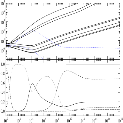
Figure 1: Cosmological evolution for a brane gas of wrapping type 8-0-2 with a solitonic flux. Top: Sizes of the spatial dimensions as functions of cosmic time. Solid curves are for unwrapped dimensions, dashed curves for partially wrapped dimensions, and dotted curves for fully wrapped dimensions. Bottom: Evolution of the different fractional contributions to the total expansion of the Universe. The solid line represents the contribution from the energy density of the M2-brane gas, the dashed line from the energy density of the gauge field, the dotted-dashed line from the energy density of supergravity particles, and the dotted line is the fractional shear component. The thick solid line is the sum of all the contributions and serves to check the accuracy of the numerical computation.

As one can observe, in this solution with eight unwrapped dimension, three spatial dimensions can get large dynamically. The energy density of the gauge field starts dominating the evolution and, consequently, four dimensions are forced to expand and six to contract initially (recall Eq. (17)). As the size of the four expanding dimensions grows, the energy density of the gauge field (9) decreases. This behaviour continues until the energy density of the brane gas takes over the rest of energy components causing the Universe to evolve with eight expanding and two contracting dimensions. After that turning point there appears a transient phase in which the energy density of the brane gas decreases and the energy density of the supergravity particles increases. This period is characterised by a fast drop of the total amount of anisotropy. The final asymmetry in the size of dimensions occurs at the time when all the energy densities stabilise.

The asymptotic behaviour of this solution can be studied analytically using a scaling ansatz of the form,

$$e^{\lambda_{i}}\sim\left\{\begin{array}[]{ll}t^{a_{+}}&\textrm{\,\,\, for }i=1,\cdots,3\\ t^{a_{-}}&\textrm{\,\,\, for }i=4,\cdots,8\\ t^{c_{-}}&\textrm{\,\,\, for }i=9\\ t^{c_{+}}&\textrm{\,\,\, for }i=10\end{array}\right.$$ (20)

The $\pm$ signs in the exponents have been introduced to keep track of the dimensions where the field strength of the gauge field is nonzero. As we have seen, the three matter components have an important fractional contribution to the expansion at late times. Imposing that all the energy densities scale with cosmic time as $t^{-2}$ and demanding selfconsistency of the Einstein equations a set of four algebraic relations can be found,

$$a_{-}-a_{+}-c_{-}+c_{+} = 0\,,$$

$$5a_{-}+3a_{+}+c_{-}+c_{+} = \frac{20}{11}\,,$$

$$3a_{+}+c_{+} = 1\,,$$

$$5a_{-}+3a_{+} = 2\,.$$

Solving for the exponents one obtains,

$$a_{+}=\frac{71}{209},\,\,\,\,a_{-}=\frac{41}{209}\,,$$

$$c_{-}=-\frac{34}{209},\,\,\,\,c_{+}=-\frac{4}{209}\,,$$

which can be compared with the numerical result,

$$a_{+}=0.33972,\,\,\,\,a_{-}=0.19614\,,$$

$$c_{-}=-0.1628,\,\,\,\,c_{+}=-0.019222\,.$$

To sum up, we have found a cosmological solution driven by a brane gas of M2-branes and a solitonic flux leading to the appropriate asymmetry among spatial dimensions with the largest number of nontrivial unwrapped dimensions allowed. Brane configurations with a large number of unwrapped dimensions can be originated after freeze out from a smaller initial size of the Universe than configurations with lower unwrapping numbers Easther et al. (2004b). In addition to the above solution we have check that other relevant solutions can also be obtain with seven and zero unwrapped dimensions. In the next sections we study a particular solution with zero unwrapped dimensions which reflects a connection between the cosmology of a brane gas in eleven dimensions and that of a string gas in ten dimensions.

II.3 Cosmological solution with wrapping 0-9-1

Now we are interested to study the asymptotic cosmological dynamics of a brane gas characterised by a wrapping of type 0-9-1 with a solitonic flux. As we will see later, this solution is the higher dimensional counterpart of the cosmological solution found in Campos (2004) for a particular ten-dimensional dilaton-gravity implementation of the Brandenberger-Vafa mechanism.

Without a gauge field, a gas of M2-branes described by a wrapping configuration that obeys the conditions $m_{1}=0$, $0<m_{3}<m_{2}$, and $2m_{2}m_{3}<25$, has the generic asymptotic power law solution (18) with,

$$b = \frac{2}{11}\frac{m_{3}+10}{m_{2}-m_{3}}\,$$

$$c = -\frac{2}{11}\frac{m_{2}+10}{m_{2}-m_{3}}\,$$

Substituting for our particular case with $m_{2}=9$ and $m_{3}=1$ one obtains,

$$b=\frac{1}{4},\,\,\,\,c=-\frac{19}{44}\,.$$ (22)

As expected, this configuration has nine dimensions which are expanding and one which is contracting. In this case both the energy density of the brane gas and the energy density of supergravity particles have a relevant contribution to the total expansion of the Universe at late times.

Let us now analyse the cosmological evolution of this brane configuration including the gauge degrees of freedom. The field strength is assumed to lay in the submanifold parametrised by the last four coordinates. Again the late attractor solution can be cast with an ansatz of the form,

$$e^{\lambda_{i}}\sim\left\{\begin{array}[]{ll}t^{b_{-}}&\textrm{\,\,\, for }i=1,\cdots,6\\ t^{b_{+}}&\textrm{\,\,\, for }i=7,8,9\\ t^{c_{+}}&\textrm{\,\,\, for }i=10\end{array}\right.$$ (23)

The numerical solution of the full equations has been plotted in Fig. 2. As one can observe, at late times only the contribution of the brane gas and the gauge field are relevant. This occurs as long as the energy density of both components scale with cosmic time as $t^{-2}$. Using the definition of these energy densities one finds two algebraic conditions,

$$3{b_{-}}+{b_{+}} = 1\,,$$

$$3{b_{+}}+{c_{+}} = 1\,.$$

On the other hand, the spatial components of Einstein equations (15) impose another additional relation,

$$2{b_{-}}+{c_{+}}=0\,.$$ (24)

Solving for ${b_{+}},{b_{-}}$ and ${c_{+}}$ the linear system of three equations, one obtains,

$${b_{+}}=\frac{5}{11},\,\,\,\,{b_{-}}=\frac{2}{11},\,\,\,\,{c_{+}}=-\frac{4}{11}\,.$$ (25)

In our numerical solution these parameters are obtained with an error of one part in $10^{4}$. Note that for this configuration the appropriate asymmetry of dimensions to explain the dimensionality of spacetime is also achieved. One direction is contracting and nine expanding with three growing more rapidly than the other six.

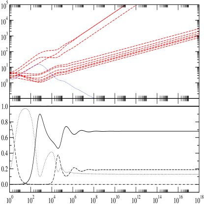
Figure 2: Cosmological evolution for a brane gas of wrapping type 0-9-1 with a solitonic flux. The identification of plots and lines is the same as in Fig. 1.

III String gas dynamics in ten dimensional dilaton-gravity

As we will see shortly the previous eleven-dimensional supergravity solution with wrapping type 0-9-1 is deeply connected with another solution in the ten-dimensional dilaton-gravity scenario for the implementation of the Brandenberger-Vafa mechanism. In particular, it is related to the string/gauge solution presented in Campos (2004). In that solution the cosmological dynamics is driven by a freezed gas of strings filling all the dimensions and a solitonic two-form gauge field. Without the dynamical effects of the flux the evolution of the string gas is completely isotropic but when it is taking into account three spatial dimensions can get large and six stabilise naturally. For simplicity, this was shown numerically for a background with three spatial dimensions. Here we complement the analysis of this solution with an analytical discussion in the appropriate number of dimensions.

III.1 Set-up

We start with the ten-dimensional bosonic action with fields only in the NS-NS sector,

$$S=\frac{1}{2\kappa^{2}_{10}}\int d^{10}x\ \sqrt{-g}e^{-2\phi}\left(R+4(\nabla_{\mu}\phi)^{2}-\frac{1}{12}H^{2}_{\alpha\beta\gamma}\right)\,,$$ (26)

where $\phi$ represents the dilaton field, $R$ is the scalar curvature of the ten-dimensional metric, and $H_{\alpha\beta\gamma}$ the field strength of the two-form gauge field. (Greek indices run from 0 to 9.) The field strength obeys two equations,

$$\nabla_{\alpha}(e^{-2\phi}H^{\alpha\beta\gamma}) = 0\,,$$ (27)

$$\nabla_{[\beta}H_{\mu\nu\alpha]} = 0\,.$$ (28)

The first comes as a result of the variation of the action with respect to the gauge degrees of freedom and the second is the Bianchi identity. Following Campos (2004), we consider a solitonic solution in which the components of the field strength are restricted to a three-dimensional spatial submanifold. By adopting a homogenous metric of the form,

$$ds^{2}=-N^{2}(t)dt^{2}+e^{2\nu(t)}\sum^{6}_{i=1}dx^{2}_{i}+e^{2\lambda(t)}\sum^{9}_{i=7}dx^{2}_{i}\,,$$ (29)

the appropriate ansatz for the flux is,

$$H^{\alpha\beta\gamma}=\frac{\epsilon^{\alpha\beta\gamma}}{\sqrt{g_{3}}}H(t)\,,$$ (30)

where, analogously to the eleven-dimensional ansatz, $g_{3}$ is the determinant of the induced three-dimensional metric and $\epsilon^{\alpha\beta\gamma}$ is the Levi-Cività antisymmetric density. In order to make a direct connection to the higher dimensional brane solution of wrapping 0-9-1, we assume the indeces $\alpha,\beta$, and $\gamma$ take values 7, 8, and 9. The above ansatz obeys the dynamical equation identically and the function $H(t)$ is actually fixed by the Bianchi identity,

$$H(t)=H_{o}e^{-3\lambda}\,,$$ (31)

where $H_{o}$ is a constant of integration. This simple solution yields a gauge term on the action that only depends on $\lambda$,

$$H^{2}_{\alpha\beta\gamma}=6H^{2}_{o}e^{-6\lambda}\equiv 12U(\lambda)\,.$$ (32)

For this solution of the gauge field, the bosonic action can be rewritten as,

$$S=\frac{1}{2\kappa^{2}_{10}}\int dte^{-\varphi}\left[\frac{1}{N}\left(3\dot{\lambda}^{2}+6\dot{\nu}^{2}-\dot{\varphi}^{2}\right)-NU(\lambda)\right]\,,$$ (33)

where we have introduced the shifted dilaton variable $\varphi\equiv 2\phi-3\lambda-6\nu$ in order to absorb the space volume factor. Taking the gauge $N=1$ and units in which $2\kappa^{2}_{10}=1$, the equations of motion are,

$$\dot{\varphi}^{2}-3\dot{\lambda}^{2}-6\dot{\nu}^{2} = e^{\varphi}E+U(\lambda)\,,$$ (34)

$$\ddot{\varphi}-3\dot{\lambda}^{2}-6\dot{\nu}^{2} = \frac{1}{2}e^{\varphi}E\,,$$ (35)

$$\ddot{\lambda}-\dot{\varphi}\dot{\lambda} = \frac{1}{2}e^{\varphi}P_{\lambda}+U(\lambda)\,,$$ (36)

$$\ddot{\nu}-\dot{\varphi}\dot{\nu} = \frac{1}{2}e^{\varphi}P_{\nu}\,.$$ (37)

In the above equations $E$ denotes the total energy of the string gas and, $P_{\lambda}$ and $P_{\nu}$ the total pressures in the three- and six-dimensional subvolumes, respectively. We are interested in a situation in which the spacetime background is still effectively higher dimensional but the strings present do not longer interact. The interaction ceases when the annihilation rate is suppressed with respect to the expansion rate. We assume that freeze-out occurs sufficiently fast and then the remaining network of strings wraps all the nine spatial dimensions. Such initial configurations are supported by recent studies of the string thermodynamics close to the Hagedorn phase Easther et al. (2004a); Danos et al. (2004). In this case, the total energy of the string gas, $E$, can be separated into the contribution from the $T^{3}$ subvolume, $E_{\lambda}$, and that of the $T^{6}$ subvolume, $E_{\nu}$,

$$E=E_{\lambda}+E_{\nu}\,.$$ (38)

For strings in a compact space these individual energies can be expressed as,

$$E_{\lambda} = \mu N_{(3)}e^{\lambda}\,,$$ (39)

$$E_{\nu} = \mu N_{(6)}e^{\nu}\,,$$ (40)

where $\mu$ is a mass parameter, and $N_{(3)}$ and $N_{(6)}$ account for the number of winding modes in the corresponding subvolume. On the other hand, the total pressure of the string gas in each subvolume are related with the above energies by,

$$P_{\lambda} = -\frac{1}{3}E_{\lambda}\,,$$ (41)

$$P_{\nu} = -\frac{1}{6}E_{\nu}\,.$$ (42)

Recall that, in general, for a nonrelativistic gas of Dp-branes in a $d$-dimensional space the total pressure is given in terms of the energy by $P=-(p/d)E$.

III.2 Late-time dynamics

Without gauge fields the above string gas set-up will certainly lead to a contracting Universe with a unique scale factor scaling as $t^{-1/5}$ at late times and consequently no asymmetry among different dimensions. Consider the opposite situation in which the energy density of the string gas is negligible. In this case the scale factors of the two subvolumes behave as,

$$e^{\lambda} \sim t^{\sqrt{3}/3}\,,$$ (43)

$$e^{\nu} \sim {\mathrm{c}onstant}\,.$$ (44)

Although a large Universe with three dimensions expanding and six dimensions stabilised seems to be explained, one can easily see that the theory becomes strongly coupled and, then, the low energy description used to describe the dynamics is inappropriate Campos (2004).

The interesting situation occurs when both the string gas and the gauge field have a significant contribution to the total expansion of the Universe at late times. Let us see that the evolution presents an attractor power-law behaviour asymptotically. One starts by taking all fields scaling with cosmic time as,

$$e^{\lambda}\sim t^{\alpha},\,\,\,\,e^{\nu}\sim t^{\beta},\,\,\,\,e^{\varphi}\sim t^{\gamma}\,.$$ (45)

To determine $\alpha$ and $\gamma$ one simply needs to look into the equation of motion for the variable $\lambda$. The right hand side of this equation can be interpreted as coming from a classical effective potential,

$$V_{eff}(\lambda)=\frac{1}{6}\left[\mu N_{(3)}e^{\varphi}e^{\lambda}+U(\lambda)\right]\,.$$ (46)

The first term comes from the string gas and produces a confinement force whereas the second term is the contribution from the gauge field and induces an expanding force. In an expanding Universe one would naively expect that the gauge contribution should always be less important than the string gas contribution. However, this does not need to be the case because the dilaton dynamics is modulating the first term in the effective potential. This means that both contributions can only be important at late times simultaneously if $\varphi$ is a decreasing function of time. This property is guaranteed by the equations of motion as long as $\dot{\varphi}$ is initially negative. Imposing that both terms in the effective potential scale asymptotically with cosmic time as $t^{-2}$ immediately yields,

$$\alpha=\frac{1}{3},\,\,\,\,\gamma=-\frac{7}{3}\,.$$ (47)

On the other hand, the consistency of the dynamical equation for $\nu$ additionally gives,

$$\beta=0\,,$$ (48)

which means that the directions that do not get large are stabilised at a constant radius. This is easily understood by examining the effective potential for the field $\nu$,

$$V_{eff}(\nu)=\frac{1}{12}\mu N_{(6)}e^{\varphi}e^{\nu}\,,$$ (49)

which represents a confining exponential force. The evolution of $\nu$ is stopped simply because the shape of the potential is completely flatten out by the dilaton field dynamics. Finally, note that with these parameters the original dilaton field behaves as $e^{\phi}\sim t^{-2/3}$ and then the weak coupling condition is dynamically preserved by this analytical solution.

Then, as a conclusion, the effect of the gauge field at late times in this string gas scenario is to make the size of three dimensions large and at the same time to stabilise the small extra dimensions giving a simple realization of the Brandenberger-Vafa mechanism.

IV Uplifting string gas solutions to eleven dimensions

Uplifting cosmological solutions from string gases in ten dimensions to eleven dimensions was briefly discussed in Easther et al. (2003). Here, we extend their discussion by considering solutions with gauge fields.

Consider the solution studied in the previous section. Asymptotically, it can be described by the ten-dimensional metric,

$$ds^{2}_{10}=-dT^{2}+\sum^{6}_{i=1}dy^{2}_{i}+T^{2\alpha}\sum^{9}_{i=7}dy^{2}_{i}\,,$$ (50)

and a late evolution for the shifted dilaton field,

$$e^{\varphi}\sim T^{\gamma}\,,$$ (51)

where $\alpha$ and $\gamma$ are given by (47). In general, the standard procedure to uplift the ten-dimensional solution to one extra dimension is to define the eleven-dimensional metric,

$$ds^{2}_{11}=e^{-2\phi/3}\,ds^{2}_{10}+e^{4\phi/3}\,dy^{2}_{10}\,,$$ (52)

where $y_{10}$ represents the tenth spatial coordinate in the higher dimensional space and $\phi$ is the original dilaton. Then, for the asymptotic cosmological solution (50), the eleven-dimensional metric should be,

$$ds^{2}_{11}=T^{-2\bar{\gamma}}\,ds^{2}_{10}+T^{4\bar{\gamma}}\,dy^{2}_{10}\,,$$ (53)

with,

$$\bar{\gamma}=\frac{1}{6}\left(\gamma+3\alpha\right)=-\frac{2}{9}\,.$$ (54)

To understand the physical meaning of this solution one has to write the metric with respect to proper time. Defining a new time coordinate $t$ as,

$$t=\frac{T^{1-\bar{\gamma}}}{1-\bar{\gamma}}\,,$$ (55)

and introducing new spatial coordinates $x_{i}$, in order to absorb irrelevant constant factors, the higher dimensional metric can be rewritten as,

$$ds^{2}_{11}=-dt^{2}+t^{-\frac{2\bar{\gamma}}{1-\bar{\gamma}}}\,\sum^{6}_{i=1}dx^{2}_{i}+t^{\frac{2(\alpha-\bar{\gamma})}{(1-\bar{\gamma})}}\,\sum^{9}_{i=7}dx^{2}_{i}+t^{\frac{4\bar{\gamma}}{1-\bar{\gamma}}}\,dx^{2}_{10}\,.$$ (56)

It is straightforward to see, by substituting the value of the parameters, that this metric corresponds to the asymptotic solution (23) and (25) described in Sec. II. This relationship permits a physical eleven-dimensional interpretation of the ten-dimensional solution. From the higher dimensional perspective, instead of a gas of strings covering the whole space with a solitonic three-form field strength, one has a M2-brane gas of anisotropic wrapping 0-9-1 with a four-form field strength. Note that the M2-brane configuration is such that all branes have one spatial dimension passing through the tenth direction which is the one that becomes compact. This is the reason why the gas of branes behaves effectively as a gas of one-dimensional objects filling the whole nine-dimensional space in the lower-dimensional gravi-dilaton implementation.

The important difference between both realizations is that from the higher dimensional point of view the compactification of the tenth dimension is obtained dynamically and not assumed a priori as being small. On the other hand, it is also worth noticing that the small dimensions that are stabilised in the dilaton-gravity context are destabilised in the M theory framework. Due to the compactification procedure this is a quite general property that makes a hard task to obtain stabilisation of the extra dimensions in the higher dimensional realization. Nevertheless, one can still imagine potential configurations that can succeed in stabilising this extra dimensions by uplifting a particular ten-dimensional solution. For instance, one can think of a set up in which the momentum modes are confined to a three dimensional subspace and a freezed gas of strings to the complementary six dimensional subspace. For this configuration one expects an asymptotic evolution with three expanding and six contracting dimensions. After uplifting to eleven dimensions the six contracting spatial dimensions can be stabilised if the dynamical evolution (45) is such that the scaling behaviour of the shifted dilaton, $\gamma$, and of the large expanding dimensions, $\alpha$, obey the condition,

$$\gamma=-3\alpha\,.$$ (57)

From the eleven-dimensional perspective three dimensions will be expanding, six will be stabilised and one, that related to the dilaton, will be contracting. Now one can ask whether a M2-brane wrapping configuration can be constructed with six, or seven if one is not interested to connect with a lower dimensional solution, asymptotically stable dimensions. To answer this question positively what seems unavoidable is the necessity of having a nonisotropic distribution of supergravity particles.

V Conclusions

This work have been devoted to present new asymptotic cosmological solutions with solitonic fluxes that could potentially explain the dimensionality of the spacetime in both the eleven-dimensional supergravity and the ten-dimensional dilaton-gravity frameworks.

In the higher dimensional context we have studied solutions supporting brane gas configurations with different numbers of unwrapped dimensions. This gives stronger evidence to the importance of fluxes, solitonic or elementary, in order to understand the full space of nontrivial solutions in brane gas cosmology. It is worth to mention that one of the solutions has eight unwrapped dimensions which is the largest possible configuration that can drive a nonisotropic cosmological evolution. This type of brane wrappings could have been produced after freeze out from a small initial volume of the Universe Easther et al. (2004b). In addition, we have also seen that solitonic and elementary fluxes introduce two different physical length scales and this will certainly be important to understand the string/brane thermodynamics of the Hagedorn phase.

We have also illustrated an example in which the lower dimensional dilaton-gravity solution is related with the M theory solution. It would be interesting to investigate whether any string gas solution in ten dimensions will have a M2-brane counterpart in eleven dimensions. One example that could be worth analysing is the string gas stabilisation mechanism proposed in Watson and Brandenberger (2003b) and find out if it has a brane gas counterpart in the eleven dimensional implementation of the Brandenberger-Vafa mechanism.

Finally, It would certainly be interesting to study the potential connection of the flux solutions we have found in the context of brane gas cosmology and the presence of S-branes Gutperle and Strominger (2002); Chen et al. (2002).