Wilson-Polchinski exact renormalization group equation for $O(N)$ systems: Leading and next-to-leading orders in the derivative expansion.† 

Abstract

With a view to study the convergence properties of the derivative expansion of the exact renormalization group (RG) equation, I explicitly study the leading and next-to-leading orders of this expansion applied to the Wilson-Polchinski equation in the case of the $N$-vector model with the symmetry $\mathrm{O}\left(N\right)$. As a test, the critical exponents $\eta$ and $\nu$ as well as the subcritical exponent $\omega$ (and higher ones) are estimated in three dimensions for values of $N$ ranging from $1$ to $20$. I compare the results with the corresponding estimates obtained in preceding studies or treatments of other $\mathrm{O}\left(N\right)$ exact RG equations at second order. The possibility of varying $N$ allows to size up the derivative expansion method. The values obtained from the resummation of high orders of perturbative field theory are used as standards to illustrate the eventual convergence in each case. A peculiar attention is drawn on the preservation (or not) of the reparametrisation invariance.

† Dedicated to Lothar Schäfer on the occasion of his 60th birthday

1 Introduction

The renormalization group (RG) theory is suitable to the study of many modern physical problems. Generically, every situation where the scale of typical physical interest belongs to a (wide) range of correlated or coupled scales may be (must be?) treated by RG techniques. Critical phenomena, which are characterized by one (or several) diverging correlation length(s), provide “the” didactic example [1]. Quantum field theory, with its strongly correlated quantum fluctuations, is not less famous since it has given rise to the early stages of the RG theory [2].

Thanks to a fortunate success (essentially due to an impressive diagrammatic calculation [3]) in estimating the critical behavior of some systems [4, 5], the perturbative framework has pushed into the background the undoubtedly nonperturbative character [6, 7, 8] of the RG theory. As a consequence, there has been relatively little interest in the development of nonperturbative RG techniques [9]. In particular the formulation of the RG theory via an infinitesimal change of the scale of reference (running scale), designated by the generic expression “exact renormalization group equation”[1] although known since 1971 [10], has actually been actively considered only since the beginning of the nineties [9]. Because the variety of systems to which the exact RG formulation could be applied is large [9, 11] (see also [12]) and also because the perturbative framework is generally not well adapted to such studies [8, 13, 14], it is worthwhile making every endeavour to master, if possible, the exact RG framework.

The exact RG equation is an integro-differential equation the study of which calls for approximations and/or truncations. Among the possible approximations, those based on expansions in powers of a small parameter such as $\epsilon=d_{u}-d$ or $1/N$ (where the upper-dimension $d_{u}=4$ for the $N$-vector model) are perturbative in essence. They, however, present the advantage of allowing analytic calculations but are attached to the smallness of quantities that are actually not small in the cases of physical interest. In some cases the perturbative framework may fail [14, 8].

The derivative expansion [15], of present interest here, is an expansion in powers of the derivative of the field. It is not associated to a small parameter though it is expected to be rather adapted to the study of phenomena at small momenta (large distances) like critical phenomena for instance. The interest of the derivative expansion is that the physical parameters (like $d$ and $N$) may take on arbitrary values. Hence, in the range of validity of the expansion (thus presumed to be in the large distance regime), the approach is actually nonperturbative. The drawback is the necessary recourse to numerical techniques [for studying coupled nonlinear ordinary differential equations (ODE)] that are not always well controlled. Consequently very few orders of the derivative expansion have really been explicitly considered.

Many studies have been effectuated in the local potential approximation (LPA), i.e. at the leading order [$O\left(\partial^{0}\right)$] of the derivative expansion [9, 11, 16]. Also, estimates of the critical exponents for Ising-like models ($N=1$) have been obtained several times from full studies of the next-to-leading order [i.e. $O\left(\partial^{2}\right)$] [15, 21, 22, 23, 24, 13], and even from a full study of the third order [$O\left(\partial^{4}\right)$] [25]. On the contrary, only two full studies have been effectuated up to $O\left(\partial^{2}\right)$ for the $\mathrm{O}\left(N\right)$ vector model [26, 27]. Yet, this model provides us with the opportunity of varying $N$  and of comparing the results with the best estimates of critical exponents obtained from six [28, 29] or seven [30] orders of the perturbative framework in a wide range of values of $N$. Interesting informations on the possible convergence of the derivative expansion are then reachable.

In the present study, I consider the $\mathrm{O}\left(N\right)$ Wilson-Polchinski exact RG equation expanded up to order $O\left(\partial^{2}\right)$ in the derivative expansion and I calculate the critical exponents. Beyond the specific calculation (which was lacking) the real aim is to try to clarify (and also to evaluate) the present status of the derivative expansion. Still, I must explain why I consider the Wilson-Polchinski equation.

Indeed, there are several different approaches and treatments of the exact RG equation so that it is not easy to really estimate the validity of the choice of the equation or/and of the calculations available in the litterature. Let me try to briefly summarize the situation and to justify my choice.

There are two families of exact RG equations (for a review see [9]). The first family expresses the RG flow ($\Lambda\mathrm{d}S_{\Lambda}/\mathrm{d}\Lambda$) of the microscopic action $S_{\Lambda}\left[\phi\right]$ (hamiltonian) associated to a running momentum scale $\Lambda$ which, in the circumstances, is a running ultra-violet cutoff. The second family expresses the RG flow of $\Gamma_{\Lambda}\left[M\right]$, the Legendre transform of $S_{\Lambda}\left[\phi\right]$, in that case the running scale $\Lambda$ effectively appears as an infra-red momentum cutoff.

There is no fundamental difference between the two families since the object of the RG is the same in the two cases: accounting for all the correlated scales $\Lambda$ ranging from 0 to $\infty$ (at criticality); only the physical meaning of the field variable at hand has been changed: $\phi$ is related to a microscopic description (like a spin of the Ising model) while $M$ is thought of as a macroscopic variable (like the magnetization). If one wants to calculate an equation of state or some correlation functions or some universal critical amplitude ratios, the second family of equations is better adapted. But if one only wants to estimate critical exponents (for example to illustrate the convergence of the derivative expansion), then considering the first family is surely more efficient. Actually, the set of ODE generated in the derivative expansion is much simpler when considered with the first family than with the second . The first family is indeed better adapted to the calculation of critical exponents for the same reason as in the field theoretical approach to critical phenomena [4], the critical exponents are defined from renormalization functions that are introduced within the microscopic action $S_{\Lambda}\left[\phi\right]$. The Wilson [1] and Polchinski [33] exact RG equations belong to the first family, they only differ by the way the smooth cutoff function has been defined (a specific function for Wilson, an arbitrary one for Polchinski). Of course, the two equations are physically equivalent, but due to a misunderstanding in the introduction of the critical exponent $\eta$ in the exact RG equation as formulated by Polchinski, it is only recently that the equivalence has been clearly established [34, 13].

If the coupled set of ODE generated by the derivative expansion is different in the two families of exact RG equations, the treatments of the differential equations encountered in the litterature differ also. For convenience, let me classify the studies in two groups according to whether the authors have adopted the conventional approach (defined below) or not.

The conventional approach is characterized as follows:

1. the set of ODE is numerically studied as such (e.g., without considering any artefact such as an expansion in powers of the field).

2. the critical exponent $\eta$ is introduced in a conventional way as defined in references [1, 35, 13].

3. the critical exponents are estimated from a set of eigenvalue equations linearized about a fixed point solution of the flow equation.

4. the reparametrization invariance is explicitly accounted for.

To limit myself to the studies mentioned above that consider $\mathrm{O}\left(N\right)$ systems via equations of the second family developped up to $O(\partial^{2})$ [26, 27]: the study of reference [26] follows the conventional approach while that of reference [27] does not. In fact, in this latter work, except the first point above, none of the other points is satisfied. This is particularly important relatively to point (iv) because the reparametrization invariance induces a line of equivalent fixed points along with $\eta$ is constant [36]. In the case where the invariance is broken (it is generally the case within the derivative expansion, except in reference [26]) then the fixed points along the line are no longer equivalents and the effective $\eta$ (when introduced conventionally) varies with the global normalisation of the field $\phi$. Nevertheless, even if the invariance is broken, one expects that a vestige of this invariance can still be observed [36, 37, 15] via an extremum of $\eta$ on varying the global normalization of the field $\phi$. The absence of explicit consideration of the reparametrization invariance in reference [27] is intringuing inasmuch as the estimation of the critical exponents is excellent (see section 3.3).

By considering the Wilson-Polchinski RG equation for $O(N)$ systems, my first aim is to illustrate the conventional treatment as described above. Additionnal aims follow:

1. Morris and Turner [26]  have imposed the reparametrization invariance by choosing a specific cutoff function and the resulting estimates of the critical exponents are not very good, especially for $\omega$. Does the Wilson-Polchinski RG equation also produce such bad results at order $O\left(\partial^{2}\right)$?.

2. Is the Wilson-Polchinski RG equation able to produce estimates of critical exponents comparable to those obtained by Gersdorff and Wetterich [27]?

3. The $\mathrm{O}\left(N\right)$ exact RG equation expanded up to order $\partial^{2}$ involves three coupled ODE. Compared to the Ising case $N=1$, it is somewhat an intermediate state between the order $\partial^{2}$ which involves two coupled equations and the order $\partial^{4}$ which involves five coupled equations [25, 20].

4. Does one observe some signs of convergence of the derivative expansion already at order $\partial^{2}$?

Relative to this latter point, it is worth mentioning here the work of Litim [38] whose aim, though very interesting, differs from that of the present work. Litim focuses its attention almost exclusively on the second family of the exact RG equations and especially on the arbitrariness introduced by the regularization process (cut-off procedure) but he does not account for the reparametrization invariance. From general arguments (independent from the derivative expansion), he provides us with a criterium for choosing the regulator which should optimize the convergence of the derivative expansion already at a very low order. The considerations are surely useful especially for studying sophisticated systems, such as gauge field theory for example, for which already the leading order of the derivative expansion is difficult to implement. However, Litim has not actually studied the convergence properties of the derivative expansion in itself but, in fact, has implicitly assumed that it converges (at least, the fact that the expansion could yield only asymptotic series has been excluded). Furthermore, Litim’s criterium of choice does not apply to the Wilson-Polchinski RG equation. In particular, at leading order of the derivative expansion, his optimization provides the same estimates of critical exponents as those obtained with the Wilson-Polchinski RG equation (see section 3.2) which, at this order, does not display any dependence on the regularization process.

2 Derivative expansion up to O$\left(\partial^{2}\right)$

2.1 Flow equations

According to reference [13], after subtraction of the high temperature fixed point $\frac{1}{2}\sum_{a=1}^{N}\int_{q}\left(\tilde{P}\psi^{2}\right)^{-1}\phi_{q}^{a}\phi_{-q}^{a}$ from the action, the Wilson-Polchinski exact RG equation satisfied by an $\mathrm{O}\left(N\right)$-symmetric action $S\left[\phi^{a}\right]$ (with $a=1,\cdots,N$) reads as follows:

$$\dot{S} = \sum_{a=1}^{N}\left\{-\int_{q}\phi_{q}^{a}\left(\tilde{d}_{\phi}\,+2q^{2}\frac{\psi^{\prime}}{\psi}+\mathbf{q}\cdot\partial_{q}\right)\frac{\delta S}{\delta\phi_{q}^{a}}\right.$$ (1)

$$\left.+\int_{q}\left(\varpi\tilde{P}-q^{2}\tilde{P}^{\prime}\right)\psi^{2}\left[\frac{\delta^{2}S}{\delta\phi_{q}^{a}\delta\phi_{-q}^{a}}-\frac{\delta S}{\delta\phi_{q}^{a}}\frac{\delta S}{\delta\phi_{-q}^{a}}\right]\right\}$$

in which $\dot{S}$ stands for $\mathrm{d}S/\mathrm{d}t=-\Lambda\mathrm{d}S/\mathrm{d}\Lambda$ (hence $\exp\left(-t\right)$ $=\Lambda/\Lambda_{0}$ in which $\Lambda_{0}$ is some initial momentum scale of reference [13]), $\mathbf{q}$ is a dimensionless $d$-vector ($d$ is the dimension of the euclidean space and $\mathbf{q}=\left\{q_{i},i=1,\cdots,d\right\}$) , $q^{2}=\sum_{i=1}^{d}q_{i}^{2}$, $\tilde{P}(q^{2})$ is a dimensionless cutoff function that decreases rapidly when $q\rightarrow\infty$ with $\tilde{P}(0)=1$ , $\psi\left(q^{2}\right)$ is an arbitrary function (except the normalization $\psi\left(0\right)=1$) introduced to test the reparametrization invariance, $\varpi=1-\eta/2$ and $\tilde{d}_{\phi}=d/2+\varpi$. A prime denotes a derivative with respect to $q^{2}$: $\psi^{\prime}=\mathrm{d}\psi/\mathrm{d}q^{2}$, $\tilde{P}^{\prime}=\mathrm{d}\tilde{P}/\mathrm{d}q^{2}$ and $\mathbf{q}\cdot\partial_{q}f\left(q\right)=\sum_{i=1}^{d}q_{i}\partial f/\partial q_{i}$.

The expansion up to order $\partial^{2}$ consists in projecting equation (1) onto actions of the form:

$${S[\phi]}={\int d^{d}x\,}\left[V{(\rho,t)+}Z{(\rho,t)(\partial\vec{\phi})^{2}+}Y{(\rho,t)(\vec{\phi}\partial\vec{\phi})^{2}}\right]$$

with

$$\rho=\frac{1}{2}\sum_{\alpha=1}^{N}\phi^{\alpha}\phi^{\alpha}=\frac{1}{2}\vec{\phi}^{2}$$

Then the flow equations for $V$, $Z$ and $Y$ read as follows:

$$\dot{V} = I_{0}\left(N{V}^{\prime}{+2\rho V}^{\prime\prime}\right)+dV-\left(d+2\varpi\right)\rho V^{\prime}-2\varpi\rho{V}^{\prime 2}$$

$$+2I_{1}\left({N}Z+2{\rho}Y\right)$$

$$\dot{Z} = I_{0}\left(NZ^{\prime}{+2\rho Z^{\prime\prime}+2}Y\right)-2\left(\varpi+1\right)Z{-}\left(d+2\varpi\right)\rho Z^{\prime}-2\psi_{0}^{\prime}V^{\prime}$$

$$-4\varpi\left({V}^{\prime}Z+\rho V^{\prime}Z^{\prime}\right)-\left[\left(\varpi-1\right)\tilde{P}_{0}^{\prime}+2\varpi\psi_{0}^{\prime}\right]V^{\prime 2}$$

$$\dot{Y} = I_{0}\left(NY^{\prime}{+2\rho}Y^{\prime\prime}{+4}Y{{}^{\prime}}\right)-(d+2+4\varpi)Y{-}\left(d+2\varpi\right)\rho Y^{\prime}-2\psi_{0}^{\prime}{V}^{\prime\prime}$$ (2)

$$-4\varpi\left({V}^{\prime\prime}Z+2{V}^{\prime}Y+\rho{V}^{\prime}Y^{\prime}+2{\rho{V}^{\prime\prime}}Y\right)$$

$$-2\left[\left(\varpi-1\right)\tilde{P}_{0}^{\prime}+2\varpi\psi_{0}^{\prime}\right]\left({V}^{\prime\prime}{V}^{\prime}+\rho{V}^{\prime\prime 2}\right)$$

in which a prime acting on $V$, $Z$ or $Y$ denotes this time a derivative with respect to $\rho$, while $\psi_{0}^{\prime}\equiv\psi^{\prime}\left(0\right)$, $\tilde{P}_{0}^{\prime}\equiv\tilde{P}^{\prime}\left(0\right)$ and:

$$I_{0}=\int_{q}\left(\varpi\tilde{P}-q^{2}\tilde{P}^{\prime}\right)\psi^{2},\qquad I_{1}=\int_{q}q^{2}\left(\varpi\tilde{P}-q^{2}\tilde{P}^{\prime}\right)\psi^{2}$$ (3)

It is convenient to perform the following changes:

$$\rho=NI_{0}\,\bar{\rho},\qquad V=NI_{0}\,\bar{V},\qquad Z=\bar{Z},\qquad Y=\frac{1}{NI_{0}}\,\bar{Y}$$ (4)

and then to consider the new set of functions:

$$\mathrm{v}_{1}=\frac{\mathrm{d}\bar{V}}{\mathrm{d}\bar{\rho}},\qquad\mathrm{v}_{2}=\bar{Z},\qquad\mathrm{v}_{3}=\bar{Y}$$

Using these new notations and restoring the writing $\bar{\rho}\longrightarrow\rho$, the set of equations (2) becomes:

$$\mathrm{\dot{v}}_{1} = \left(1+\frac{{2}}{N}\right)\mathrm{v}_{1}^{\prime}{+}\frac{{2}}{N}{\rho\mathrm{v}_{1}^{\prime\prime}}-e\mathrm{v}_{1}-\left(d+e\right)\rho\mathrm{v}_{1}^{\prime}-e\left(\mathrm{v}_{1}^{2}+2\rho\mathrm{v}_{1}\mathrm{v}_{1}^{\prime}\right)$$ (5)

$$+P_{1}\left[\mathrm{v}_{2}^{\prime}+\frac{2}{N}\left(\mathrm{v}_{3}+{\rho}\mathrm{v}_{3}^{\prime}\right)\right]$$

$$\mathrm{\dot{v}}_{2} = \mathrm{v}_{2}^{\prime}{+}\frac{{2}}{N}{\rho\mathrm{v}_{2}^{\prime\prime}+}\frac{{2}}{N}\mathrm{v}_{3}-\left(e+2\right)\mathrm{v}_{2}{-}\left(d+e\right)\rho\mathrm{v}_{2}^{\prime}+2u\mathrm{v}_{1}$$ (6)

$$-2e\left(\mathrm{v}_{1}\mathrm{v}_{2}+\rho\mathrm{v}_{1}\mathrm{v}_{2}^{\prime}\right)+P_{2}\mathrm{v}_{1}^{2}$$

$$\mathrm{\dot{v}}_{3} = \left(1+\frac{{4}}{N}\right)\mathrm{v}_{3}^{\prime}{+}\frac{{2}}{N}{\rho}\mathrm{v}_{3}^{\prime\prime}-(d+2+2e)\mathrm{v}_{3}{-}\left(d+e\right)\rho\mathrm{v}_{3}^{\prime}+2u\mathrm{v}_{1}^{\prime}$$ (7)

$$-2e\left[\mathrm{v}_{1}^{\prime}\left(\mathrm{v}_{2}+2{\rho}\mathrm{v}_{3}\right)+\mathrm{v}_{1}\left(2\mathrm{v}_{3}+\rho\mathrm{v}_{3}^{\prime}\right)\right]+2P_{2}\left(\mathrm{v}_{1}+\rho\mathrm{v}_{1}^{\prime}\right)\mathrm{v}_{1}^{\prime}$$

in which:

$$u = -\psi_{0}^{\prime},\qquad e=2\varpi\qquad$$

$$P_{1} = 2\frac{I_{1}}{I_{0}},\qquad P_{2}=-\left(\frac{e}{2}-1\right)\tilde{P}^{\prime}(0)+eu$$

2.2 Fixed point equations

The fixed point equations correspond to the three simultaneous conditions $\mathrm{\dot{v}}_{i}=0$ for $i=1,2,3$ which yield three coupled nonlinear ODE of second order each:

$${\mathrm{v}_{1}^{\prime\prime}} = \frac{N}{2\rho}\left[e\mathrm{v}_{1}\left(1+\mathrm{v}_{1}\right)-\left(1+\frac{{2}}{N}\right)\mathrm{v}_{1}^{\prime}-P_{1}\left(\mathrm{v}_{2}^{\prime}+\frac{2}{N}\mathrm{v}_{3}\right)\right]$$ (8)

$$+\frac{N}{2}\left(d+e+2e\mathrm{v}_{1}\right)\mathrm{v}_{1}^{\prime}-P_{1}\mathrm{v}_{3}^{\prime}$$

$${\mathrm{v}_{2}^{\prime\prime}} = \frac{N}{2\rho}\left[\left(e+2+2e\mathrm{v}_{1}\right)\mathrm{v}_{2}-\mathrm{v}_{2}^{\prime}{-}\frac{{2}}{N}\mathrm{v}_{3}-2u\mathrm{v}_{1}-P_{2}\mathrm{v}_{1}^{2}\right]$$ (9)

$$+\frac{N}{2}\left[\left(d+e\right){+}2e\mathrm{v}_{1}\right]\mathrm{v}_{2}^{\prime}$$

$$\mathrm{v}_{3}^{\prime\prime} = \frac{N}{2\rho}\left[\left(d+2+2e+4e\mathrm{v}_{1}\right)\mathrm{v}_{3}-\left(1+\frac{{4}}{N}\right)\mathrm{v}_{3}^{\prime}+2\left(e\mathrm{v}_{2}-u-P_{2}\mathrm{v}_{1}\right)\mathrm{v}_{1}^{\prime}\right]$$ (10)

$${+}\frac{N}{2}\left[\left(d+e+2e\mathrm{v}_{1}\right)\mathrm{v}_{3}^{\prime}+2\left(2e\mathrm{v}_{3}-P_{2}\mathrm{v}_{1}^{\prime}\right)\mathrm{v}_{1}^{\prime}\right]$$

The differential system is of order six, thus the general solution depends on six arbitrary constants. Three of these constants are fixed so as to avoid the singularity at the origin $\rho=0$ displayed by the equations, hence the three following conditions:

$$\mathrm{v}_{2}^{\prime}\left(0\right) = \left[e+2+2e\mathrm{v}_{1}\left(0\right)\right]\mathrm{v}_{2}\left(0\right){-}\frac{{2}}{N}\mathrm{v}_{3}\left(0\right)-\mathrm{v}_{1}\left(0\right)\left[2u+P_{2}\mathrm{v}_{1}\left(0\right)\right]$$ (11)

$$\mathrm{v}_{1}^{\prime}\left(0\right) = \frac{N}{N+2}\left\{e\mathrm{v}_{1}\left(0\right)\left[1+\mathrm{v}_{1}\left(0\right)\right]-P_{1}\left[\mathrm{v}_{2}^{\prime}\left(0\right)+\frac{2}{N}\mathrm{v}_{3}\left(0\right)\right]\right\}$$ (12)

$$\mathrm{v}_{3}^{\prime}\left(0\right) = \frac{N}{N+4}\left\{\left[d+2+2e+4e\mathrm{v}_{1}\left(0\right)\right]\mathrm{v}_{3}\left(0\right)\right.$$ (13)

$$\left.+2\left[e\mathrm{v}_{2}\left(0\right)-u-P_{2}\mathrm{v}_{1}\left(0\right)\right]\mathrm{v}_{1}^{\prime}\left(0\right)\right\}$$

If $\eta$ is a priori fixed, then the general solution of the set of equations (8–10) depends on the three remaining arbitrary constants, e.g. the values $\mathrm{v}_{i}\left(0\right)$ for $i=1,2,3$. In general the corresponding solutions are singular at some varying $\rho^{\ast}$ (moving singularity), with:

$$\mathrm{v}_{1}\left(\rho\right)\propto\left(\rho^{\ast}-\rho\right)^{-1},\qquad\mathrm{v}_{2}\left(\rho\right)\propto\left(\rho^{\ast}-\rho\right)^{-2},\qquad\mathrm{v}_{3}\left(\rho\right)\propto\left(\rho^{\ast}-\rho\right)^{-2}$$

But, the equations (8–10) admit another kind of solution that goes to infinity ($\rho\rightarrow\infty$) without encountering any singularity and which behaves asymptotically for large $\rho$ as follows:

$$\mathrm{v}_{1\mathrm{asy}}\left(\rho\right) = G_{1}\rho^{\theta_{1}}+\left(1+2\theta_{1}\right)G_{1}^{2}\rho^{2\theta_{1}}+\cdots$$ (14)

$$\mathrm{v}_{2\mathrm{asy}}\left(\rho\right) = uG_{1}\rho^{\theta_{1}}+G_{1}^{2}\,\left(1+{{\theta}_{1}}\right)\frac{2\,\left(d\,-\,e\right)\,u+\left(d\,+e\,\right){\tilde{P}}_{0}^{\prime}}{2\,d}\rho^{2\theta_{1}}$$ (15)

$$+G_{2}\rho^{\theta_{2}}+\cdots$$

$$\mathrm{v}_{3\mathrm{asy}}\left(\rho\right) = u\theta_{1}G_{1}\rho^{\theta_{1}-1}+2G_{1}^{2}\,{{\theta}_{1}}\,\frac{2\,\left(d\,-\,e\right)\,u+d\,{\tilde{P}}^{\prime}{{}_{0}}}{2\,\left(d+e\right)}\rho^{2\theta_{1}-1}$$ (16)

$$+G_{3}\rho^{\theta_{3}}+\cdots$$

with:

$$\theta_{1}=-\frac{e}{d+e},\qquad\theta_{2}=-\frac{e+2}{d+e},\qquad\theta_{3}=\theta_{2}-1$$

The values of the three constants $\left\{G_{i};i=1,2,3\right\}$, correspond to some adjustment of the set $\left\{\mathrm{v}_{i}\left(0\right);i=1,2,3\right\}$ and vice versa. This nonsingular solution is the fixed point solution which we are interested in. When $\eta$ is a priori fixed, the six arbitrary constants of integration are then determined, the differential system is balanced.

If $\eta$ is considered as an unknown parameter to be determined, then one of the three preceding quantities $\left\{\mathrm{v}_{i}\left(0\right)\right\}$ or $\left\{G_{i}\right\}$ must be promoted to the rank of a fixed parameter chosen a priori. In general one chooses

$$\mathrm{v}_{2}\left(0\right)=Z_{0}$$ (17)

which corresponds to having fixed to $Z_{0}$ the value of the kinetic term in $S\left[\phi^{a}\right]$ and is customarily associated with the arbitrary global normalization of the field $\phi$. One thus obtains a function $\eta\left(Z_{0}\right)$ which should be a constant if the reparametrization invariance of the exact RG equation was preserved by the derivative expansion presently considered ($\eta$ should be a constant along a line of equivalent fixed points generated by the variation of $Z_{0}$). Since it is not the case, one actually obtains a nontrivial function $\eta\left(Z_{0}\right)$. Fortunately a vestige of the reparametrisation invariance is preserved and $\eta\left(Z_{0}\right)$ displays an extremum in $Z_{0}$. This provides us with an optimal value ($\eta^{\mathrm{opt}}$) of $\eta$ (and similarly for $Z_{0}$) via the condition:

$$\frac{\mathrm{d}\eta^{\mathrm{opt}}}{\mathrm{d}Z_{0}}=0$$ (18)

Instead of using this condition to determine $\eta^{\mathrm{opt}}$, I use the fact that the line of equivalent fixed points is associated with a redundant operator with a zero eigenvalue [36, 37]. Hence, one may determine $\eta^{\mathrm{opt}}$ by imposing that the fixed point of interest be associated to a zero eigenvalue. This leads us to the consideration of the system of eigenvalue equations.

2.3 Eigenvalue equations

The eigenvalue equations are obtained by linearization of the flow equations (5–7) about a fixed point solution $\left\{\mathrm{v}_{i}^{\mathrm{\ast}},i=1,2,3\right\}$:

$$\mathrm{v}_{i}=\mathrm{v}_{i}^{\mathrm{\ast}}+\varepsilon\mathrm{e}^{\lambda t}\mathrm{g}_{i}$$

Keeping the linear contribution in $\varepsilon$, the following set of coupled ODE comes:

$$\mathrm{g}_{1}^{\prime\prime} = \frac{N}{2\rho}\left[\left(\lambda+e+2e\mathrm{v}_{1}^{\mathrm{\ast}}\right)\mathrm{g}_{1}-\left(1+\frac{{2}}{N}\right)\mathrm{g}_{1}^{\prime}-P_{1}\left(\mathrm{g}_{2}^{\prime}+\frac{2}{N}\mathrm{g}_{3}\right)\right]$$ (19)

$$+\frac{N}{2}\left[\left(d+e+2e\mathrm{v}_{1}^{\mathrm{\ast}}\right)\mathrm{g}_{1}^{\prime}+2e\mathrm{g}_{1}\mathrm{v}_{1}^{\mathrm{\ast}\prime}\right]-P_{1}\mathrm{g}_{3}^{\prime}$$

$${\mathrm{g}_{2}^{\prime\prime}} = \frac{N}{2\rho}\left[\left(\lambda+e+2+2e\mathrm{v}_{1}^{\mathrm{\ast}}\right)\mathrm{g}_{2}-\mathrm{g}_{2}^{\prime}{-}\frac{{2}}{N}\mathrm{g}_{3}+2\left(e\mathrm{v}_{2}^{\ast}-u-P_{2}\mathrm{v}_{1}^{\mathrm{\ast}}\right)\mathrm{g}_{1}\right]$$ (20)

$${+}\frac{N}{2}\left[\left(d+e+2e\mathrm{v}_{1}^{\mathrm{\ast}}\right)\mathrm{g}_{2}^{\prime}+2e\mathrm{g}_{1}\mathrm{v}_{2}^{\ast\prime}\right]$$

$$\mathrm{g}_{3}^{\prime\prime} = \frac{N}{2\rho}\left[(\lambda+d+2+2e+4e\mathrm{v}_{1}^{\ast})\mathrm{g}_{3}-\left(1+\frac{{4}}{N}\right)\mathrm{g}_{3}^{\prime}-2u\mathrm{g}_{1}^{\prime}\right.$$ (21)

$$\left.+2e\left(\mathrm{g}_{1}^{\prime}\mathrm{v}_{2}^{\ast}+2\mathrm{g}_{1}\mathrm{v}_{3}^{\ast}\right)-2P_{2}\left(\mathrm{g}_{1}\mathrm{v}_{1}^{\ast\prime}+\mathrm{v}_{1}^{\ast}\mathrm{g}_{1}^{\prime}\right)+2e\mathrm{v}_{1}^{\ast\prime}\mathrm{g}_{2}\right]$$

$${+}\frac{N}{2}\left[\left(d+e+2e\mathrm{v}_{1}^{\mathrm{\ast}}\right)\mathrm{g}_{3}^{\prime}+2e\left(2\mathrm{g}_{1}^{\prime}\mathrm{v}_{3}^{\ast}+\mathrm{g}_{1}\mathrm{v}_{3}^{\ast\prime}+2\mathrm{v}_{1}^{\ast\prime}\mathrm{g}_{3}\right)-4P_{2}\mathrm{g}_{1}^{\prime}\mathrm{v}_{1}^{\ast\prime}\right]$$

Similar considerations as those relative to the determination of the six integration constants associated to the fixed point equations (8–10) stand. For a given fixed point solution ($\mathrm{v}_{i}^{*}$), there remain six constants to be determined. Three of them are fixed so as to avoid the singularity at the origin $\rho=0$ displayed by the equations:

$$\mathrm{g}_{2}^{\prime}\left(0\right) = \left[\lambda+e+2+2e\mathrm{v}_{1}^{\mathrm{\ast}}\left(0\right)\right]\mathrm{g}_{2}\left(0\right){-}\frac{{2}}{N}\mathrm{g}_{3}\left(0\right)$$

$$+2\left[e\mathrm{v}_{2}^{\ast}\left(0\right)-u-P_{2}\mathrm{v}_{1}^{\mathrm{\ast}}\left(0\right)\right]\mathrm{g}_{1}\left(0\right)$$

$$\mathrm{g}_{1}^{\prime}\left(0\right) = \frac{N}{N+2}\left\{\left[\lambda+e+2e\mathrm{v}_{1}^{\mathrm{\ast}}\left(0\right)\right]\mathrm{g}_{1}\left(0\right)-P_{1}\left[\mathrm{g}_{2}^{\prime}\left(0\right)+\frac{2}{N}\mathrm{g}_{3}\left(0\right)\right]\right\}$$

$$\mathrm{g}_{3}^{\prime}\left(0\right) = \frac{N}{N+4}\left\{\left[\lambda+d+2+2e+4e\mathrm{v}_{1}^{\ast}\left(0\right)\right]\mathrm{g}_{3}\left(0\right)-2u\mathrm{g}_{1}^{\prime}\left(0\right)\right.$$

$$+2e\left[\mathrm{g}_{1}^{\prime}\left(0\right)\mathrm{v}_{2}^{\ast}\left(0\right)+2\mathrm{g}_{1}\left(0\right)\mathrm{v}_{3}^{\ast}\left(0\right)\right]$$

$$\left.-2P_{2}\left[\mathrm{g}_{1}\left(0\right)\mathrm{v}_{1}^{\ast\prime}\left(0\right)+\mathrm{v}_{1}^{\ast}\left(0\right)\mathrm{g}_{1}^{\prime}\left(0\right)\right]+2e\mathrm{v}_{1}^{\ast\prime}\left(0\right)\mathrm{g}_{2}\left(0\right)\right\}$$

One is interested in the solution that is regular when $\rho\rightarrow\infty$.

For $\lambda$ a priori fixed, the three values $\left\{\mathrm{g}_{i}\left(0\right),i=1,2,3\right\}$ at the origin $\rho=0$ must be adjusted so that the solution reaches the following regular asymptotic behavior:

$$\mathrm{g}_{1\mathrm{asy}} = S_{1}\rho^{\chi_{1}}+2\,\,\left(1+{{\theta}_{1}+}\chi_{1}\right)\,{G_{1}}\,{S_{1}\rho}^{{{\theta}_{1}+}\chi_{1}}+\cdots$$

$$\mathrm{g}_{2\mathrm{asy}} = S_{2}\rho^{\chi_{2}}+uS_{1}\rho^{\chi_{1}}+\cdots$$

$$\mathrm{g}_{3\mathrm{asy}} = S_{3}\rho^{\chi_{3}}+uS_{1}\chi_{1}\rho^{\chi_{1}-1}+\cdots$$

with:

$$\chi_{1}=-\frac{\lambda+e}{d+e},\qquad\chi_{2}=-\frac{\lambda+e+2}{d+e},\qquad\chi_{3}=\chi_{2}-1$$

and the value of the set of constants $\left\{S_{i},i=1,2,3\right\}$ entering the regular solution at large $\rho$ corresponds to the value of $\left\{\mathrm{g}_{i}(0)\right\}$ adjusted at the origin and vice versa.

As in any eigenvalue problem, the global normalization of the eigenvector may be chosen at will so that, fixing $\mathrm{g}_{1}\left(0\right)=1$ for instance, allows one to determine discrete values of $\lambda$. Positive values give the critical exponents, negative values are subcritical (or correction-to-scaling) exponents.

The peculiar value $\lambda=0$, if present, is associated to the vestige of the reparametrization invariance [37, 15]. Indeed this zero eigenvalue is associated to the redundant operator that generates the line of equivalent fixed points in the complete theory [36, 37]. Conversely, if one considers together the fixed point equations (8–10) with the eigenvalue equations (19–21) in which $\lambda$ is set equal to zero (and the condition $\mathrm{g}_{1}\left(0\right)=1$ is maintained), then the condition (17) may be abandoned and $\mathrm{v}_{2}\left(0\right)$ adjusted so as to get a common solution to the set of six coupled ODE. Then, the resulting value of $\eta$ nececessarily coincides with $\eta^{\mathrm{opt}}$ as defined by equation (18) and the resulting value of $\mathrm{v}_{2}(0)$ gives $Z_{0}^{\mathrm{opt}}$. Though the number of differential equations has increased twofold this procedure of determining the optimized fixed point is the most efficient one when parameters (like $N$ and some other ones, see following section) have to be varied.

2.4 The free parameters

In order to perform an actual numerical study of the set of second order ODE described in the preceding section, I make the following choice :

$$\tilde{P}\left(q^{2}\right) = \mathrm{e}^{-q^{2}}$$ (22)

$$\psi\left(q^{2}\right) = \frac{1}{1+bq^{2}}$$ (23)

Following the terminology of reference [39], the free parameter $b$ is redundant and is intended to be used to optimize the numerical results of the derivative expansion.

The introduction of $b$ is linked to the general property of reparametrization invariance which is broken by the present derivative expansion. The normalization $\psi\left(0\right)=1$ is chosen in order to distinguish the effect of simply changing the global normalization of the field which induces a line of equivalent fixed points (at fixed $b$). That line is customarily associated to the arbitrariness of $Z_{0}$ the value of $Z\left(0\right)$ ($\equiv\mathrm{v}_{2}\left(0\right)$), i.e. the coefficient of the kinetic term in $S\left[\phi^{a}\right]$ (see preceding section). Changing the value of $b$ in the complete theory would induce new (equivalent) lines of equivalent fixed points.

Though they are part of the same invariance, the two free parameters $b$ and $Z_{0}$ have effects of different nature in the derivative expansion. As a global constant of normalization, one can expect that, at a given order of the derivative expansion, the variation of $Z_{0}$ will still reveal a vestige of the invariance of the exact theory (see preceding section). On the contrary, the effect of $b$ spreads out over different orders of the derivative expansion. Consequently, one expects to observe a progressive restoration of the redundant character of $b$ as the order of the expansion increases. Regarding the extremely low order considered here ($\mathrm{O}\left(\partial^{2}\right)$), one must not expect too much from varying $b$ (see section 3.2).

Notice that the cutoff function $\tilde{P}\left(q^{2}\right)$ is essentially a regulator of the integrals (3) generated by the derivative expansion. Besides the arbitrary choice in the decreasing at large $q$, the other sources of arbitrariness of the cutoff function may be included within the arbitrary function $\psi\left(q^{2}\right)$. This is why the choice (22) does not involve any free parameter.

3 Numerical study and results

There are two different methods for numerically studying systems of coupled nonlinear ODE as those described above: the shooting and the relaxation methods (see, for example reference [40]). Because it is the easiest to implement, only the shooting method is considered here (though it is less numerically stable than the relaxation method).

3.1 The shooting method

Considering an initial point $\rho_{1}$ where known conditions (initial conditions) are imposed and trial values are given to the remaining integration constants, one integrates the ODE system up to a second point $\rho_{2}$ where the required conditions are checked. Using a Newton-Raphson algorithm, one iterates the test until the latter conditions are satisfied within a given accuracy.

In the present study, the two points $\rho_{1}$ and $\rho_{2}$ are either the origin $\rho=0$ and a large value $\rho_{\mathrm{asy}}$ (shooting from the origin) or the reverse (shooting to the origin).

In principle, shooting to the origin is technically better adapted to the present study. For example, in the case of the fixed point equations (8–10) with $\eta$ fixed, one starts from $\rho_{\mathrm{asy}}$ with trial values for the three constants $\left\{G_{i}\right\}$ and the initial values of the three functions and of their first derivatives $\left\{\mathrm{v}_{i},\mathrm{v}_{i}^{\prime}\right\}$ defined by (14–16). After integration up to the origin, one checks whether the three conditions (11–13) are fulfilled or not. The system is balanced and the values of the other interesting parameters are simply by-products of the adjustment. For example, the value of $Z_{0}$ associated to the arbitrarily fixed value of $\eta$ is simply read as the value that $\mathrm{v}_{2}\left(0\right)$ takes on after achievement of the adjustment. If one wants instead to determine $\eta\left(Z_{0}\right)$, then $\eta$ has to be considered as a trial parameter like $\left\{G_{i}\right\}$ and the supplementary condition (17) with $Z_{0}$ an arbitrary fixed number, must be fulfilled at the origin.

Unfortunately, equations (8–10) are singular at $\rho=0$ so that it is impossible to shoot to the origin. In reference [41] (where the leading order LPA was studied for small values of $N$), the difficulty was circumvented by shooting to a point close to the origin. On the contrary, I have chosen to shoot from the origin because it is easy to control the equations starting from that point.

Starting from the origin implies that, for a given value of $\eta$, the adjustable parameters no longer are the $\left\{G_{i}\right\}$ but the initial values $\left\{\mathrm{v}_{i}\left(0\right)\right\}$, the initial values of the first derivatives follow from (11–13). At the point $\rho_{\mathrm{asy}}$ only three conditions are needed in order to balance the number of adjustable parameters. Thus one must eliminate the $\left\{G_{i}\right\}$ from the six equations (14–16) to obtain three anonymous conditions. Consequently the precise knowledge of the asymptotic behavior of the regular fixed point solution is not necessary.

It appears that imposing conditions like $\left\{\mathrm{v}_{i}^{\prime\prime}\left(\rho_{\mathrm{asy}}\right)=0\right\}$ is sufficient to determine the solution of interest. I first adjust the trial parameters so as to reach some not too large a value of $\rho_{\mathrm{asy}}$, then I increase $\rho_{\mathrm{asy}}$ until the desired accuracy is reached on the trial parameters.

3.2 Numerical results

Table 1: Critical exponent estimates (for $d=3$) from the $\mathrm{O}\left(N\right)$ Wilson-Polchinski exact RG equation expanded up to $O\left(\partial^{2}\right)$ in the derivative expansion for two values of the free parameter $b$.

• 	$b=0.03$			$b=0.11$
  $N$	$\eta$	$\nu$	$\omega$	$\eta$	$\nu$	$\omega$
  $1$	$0.01006$	$0.6223$	$0.7755$	$0.02494$	$0.5994$	$0.8740$
  $2$	$0.00866$	$0.6723$	$0.7266$	$0.02263$	$0.6388$	$0.7656$
  $3$	$0.00721$	$0.7238$	$0.7132$	$0.02007$	$0.6838$	$0.7156$
  $4$	$0.00592$	$0.7713$	$0.7223$	$0.01739$	$0.7313$	$0.7010$
  $5$	$0.00486$	$0.8111$	$0.7437$	$0.01489$	$0.7762$	$0.7088$
  $6$	$0.00404$	$0.8424$	$0.7695$	$0.01275$	$0.8138$	$0.7307$
  $7$	$0.00342$	$0.866$	$0.7946$	$0.01100$	$0.8440$	$0.7576$
  $8$	$0.00294$	$0.8849$	$0.8172$	$0.00960$	$0.8673$	$0.7842$
  $9$	$0.00256$	$0.8993$	$0.8368$	$0.00848$	$0.8854$	$0.8081$
  $10$	$0.00227$	$0.9107$	$0.8533$	$0.00757$	$0.8995$	$0.8292$
  $11$	$0.00204$	$0.9214$	$0.8711$	$0.00683$	$0.9108$	$0.8463$
  $12$	$0.00184$	$0.9293$	$0.8836$	$0.00621$	$0.9198$	$0.8613$
  $15$	$0.00142$	$0.9438$	$0.9060$	$0.00488$	$0.9387$	$0.8942$
  $20$	$0.00102$	$0.9596$	$0.9330$	$0.00358$	$0.9563$	$0.9258$

Table 2: Same as table 1 (two other values of $b$).

• 	$b=0.17011$			$b=0.25611$
  $N$	$\eta$	$\nu$	$\omega$	$\eta$	$\nu$	$\omega$
  $1$	$0.03553$	$0.5850$	$0.9515$	$0.04979$	$0.5677$	$1.0906$
  $2$	$0.03278$	$0.6176$	$0.7917$	$0.04670$	$0.5908$	$0.8273$
  $3$	$0.02980$	$0.6574$	$0.7115$	$0.04371$	$0.6242$	$0.7288$
  $4$	$0.02643$	$0.7033$	$0.6806$	$0.03999$	$0.6664$	$0.6570$
  $5$	$0.02300$	$0.7506$	$0.6809$	$0.03565$	$0.7175$	$0.6538$
  $6$	$0.01986$	$0.7939$	$0.7040$	$0.03175$	$0.7737$	$0.6682$
  $7$	$0.01719$	$0.8291$	$0.7331$	$0.02772$	$0.8224$	$0.7137$
  $8$	$0.01502$	$0.8565$	$0.7641$	$0.02352$	$0.8565$	$0.7456$
  $9$	$0.01327$	$0.8779$	$0.7938$	$0.02150$	$0.8928$	$0.8037$
  $10$	$0.01185$	$0.8944$	$0.8194$	$0.01937$	$0.9132$	$0.8165$
  $11$	$0.01068$	$0.9075$	$0.8413$	$0.01734$	$0.9357$	$0.8505$
  $12$	$0.00972$	$0.9180$	$0.8596$	$0.01588$	$0.9552$	$0.8741$
  $15$	$0.00779$	$0.9552$	$0.9209$	—	—	—

Table 3: Compared to LPA on the lhs of the arrows, the order $\partial^{2}$ (rhs of the arrows) induces a splitting into two of the subcritical exponents of degree higher than $\omega$ (values for $d=3$, $N=1$ and $b=0.11$). The LPA values may be found in [43].

• $\omega$	$\omega_{2}$	$\omega_{3}$	$\omega_{4}$
  $0.6557\rightarrow 0.8740$	$3.18\rightarrow\left\{\begin{array}[]{l}2.83\\ 3.62\end{array}\right.$	$5.91\rightarrow\left\{\begin{array}[]{l}5.70\\ 6.40\end{array}\right.$	$8.80\rightarrow\left\{\begin{array}[]{l}7.30\\ 9.6\end{array}\right.$

At the leading order LPA, the function $\mathrm{v}_{1}$ is considered alone. Only one second order ODE defines the fixed point (twice this number for the eigenvalue problem). The study has already been done in reference [41] for $d=3$ and $N=1$ to $4$. I have extended the results (for $d=3$) to larger values of $N$. The study is simple because:

1. the reparametrization invariance is automatically satisfied since, by construction, the coefficient of the kinetic term is supposed to be constant.

2. the equation (5) with $\mathrm{v}_{2}=\mathrm{v}_{3}=0$, does not depend on any free parameter like $b$.

Consequently there is no ambiguity: to any value of $N$, corresponds a unique value of $\nu$ and $\omega$ while $\eta$=0. As already mentioned in reference [42], it is noteworthy that the values I obtain (see also [41]) for the critical and subcritical exponents (without optimization since there is no free parameters at hand) agree, “to all published digits”, with the “optimized” values obtained in reference [43] from a study of an exact RG equation of the second family. Hence, for the numerical results I have obtained at order LPA for $\nu$, $\omega$ and other subleading critical exponents $\omega_{n}$, the reader is referred to table 1 of reference [43].

At order $\partial^{2}$, once the arbitrariness of $Z_{0}$ has been removed via the definition of $\eta^{\mathrm{opt}}$, the values of the critical exponents still depend on $b$ in such a way that, for a given value of $N$, it is impossible to define “preferred” values. For example $\eta$ (from now on, $\eta$ stands for $\eta^{\mathrm{opt}}$) depends on $b$ almost linearly.

Due to the spreading out over several orders of the effects of $b$, the study of the convergence of the derivative expansion relies rather on the consideration of several orders. Now the order $\partial^{2}$ is still too low to allow an appreciation of the convergence of the derivative expansion. Instead of presently producing one “best” estimate for each critical exponent at a given value of $N$, it is preferable to maintain the freedom of $b$ in order to better emphasize the early beginnings of some criteria of convergence if any (see section 3.3).

Tables 1 and 2 display the estimates of $\eta$, $\nu$ and $\omega$ as obtained for four values of $b$ and $N$ varying from 1 to 20 (while $d=3$).

For $N=1$, the results of reference [13] (preferred value of $\eta^{\mathrm{opt}}$ for $b=0.11$) is obtained again. In this latter work I had proposed a criterium of choice of the value of $b$ which gave a preferred value of $\eta$. It was based on the idea of Golner [15] of a global minimization of the magnitude of the function $Z\left(\phi\right)$ (i.e., $\mathrm{v}_{2}\left(\phi\right)$). However the extension of this criterion to $N>1$ is not easy to implement because the function $Z\left(\phi\right)$ has been split into two parts ($Z(\rho)$ and $Y(\rho)$).

The further discussion of these results is left to section 3.3.

Table 3 displays a comparison between the LPA and $O(\partial^{2})$ results for $d=3$, $N=1$ and $b=0.11$ of the series of subcritical exponents $\omega_{n}$ (with $\omega_{1}=\omega$). Compared to LPA, the order $O\left(\partial^{2}\right)$ has increased the potential number of subcritical exponents (due to the supplementary terms in the truncated action considered). For instance, if one adopts the dimensional analysis of perturbation theory, then at order LPA a term like $\phi^{6}$ contributing to $S[\phi]$ is associated with the subcritical $\omega_{2}$ while a $\phi^{8}$-term generates $\omega_{3}$. But at order $O\left(\partial^{2}\right)$, new terms involving two derivatives contribute to $S[\phi]$, and a term proportionnal to $\phi^{2}(\partial\phi)^{2}$ induces a priori an in-between correction exponent. Despite important differences between the classical dimensions of the couples $\phi^{6}$ and $\phi^{2}(\partial\phi)^{2}$, table 3 clearly shows that, for $N=1$, the order $\partial^{2}$ induces a splitting of the LPA values of the subcritical exponents $\omega_{n}$ for $n>1$ ($\omega$ is, in the perturbative approach, associated to the unique $\phi^{4}$ coupling and is not, fortunately for the perturbative framework, subject to this splitting). This simple splitting is presumably not preserved for other values of $N$ due to the supplementary contribution of $Y(\phi)$.

3.3 Comparison with other studies, discussions and conclusion

Figure 1 shows the evolution of $\eta$ with $N$ from different works. The results obtained from the resummation of six [29] and seven [30] orders of the perturbation field theory serves the purpose of standards (other accurate estimates of the critical exponents, especially for $N\leq 4$, exist in the litterature, for a review see [5]). One sees that the present study yields generally small values of $\eta$ compared to the standards except for small $N$ and for the highest values of $b$. The evolution of $\eta$ with $N$ is smoother than in the work of Morris and Turner [26] but, as in this latter work, the non-monotonic behavior of the standards (responsible for the maximum of $\eta$ about $N=2$ or $3$) is not reproduced. Instead, the results of Gersdorff and Wetterich [27] are better. The present results are however not so bad if one keeps in mind that the first estimate of $\eta$ in the derivative expansion is given at order $\partial^{2}$. In particular, figure 1 shows also recent estimates from the resummation of three orders of the perturbative series using an efficient method [44]. One sees that the present estimates withstand the comparison (except the monotonic evolution with $N$). Notice also, for $N$ fixed, the monotonic evolution of $\eta$ with $b$ already mentioned.

The results for the critical exponent $\nu$ are more interesting to discuss because the order $\partial^{2}$ provides its second estimate. Figure 2 shows the evolution with $N$ of $\nu$ at order $\partial^{2}$ compared to the results at order LPA (obtained in the present work), the standards [29, 30] are reproduced also. Again, one observes that the results for large $N$ are not as good as for small values. However, for these latter values, one clearly sees that there is a range of values of $b$ where the two estimates at orders LPA and $\partial^{2}$ flank the standards and another range where the two present estimates are on the same side (with respect to the standards). This is a phenomenon often observed in convergent series the elements of which depend on a free parameter (like $b$) but the resumed series does not: on varying the free parameter, one may observe monotonic or alternate approaches to the limit. These features may be used to determine error bars. Presently one additionnal order would be necessary to propose such error bars. Figure 2 shows also that, when $N$ increases the dependence of $\nu$ on $b$ becomes non-monotonic. This is interesting since such extrema may indicate a vestige of the primarily independence on $b$ of the exact RG equation. Why this effect does not occur at small values of $N$ is not explained. Once more, at least one supplementary order of the derivative expansion would be necessary to understand this point.

Figure 3 shows the results for $\nu$ coming from [26] and [27] compared to the present results for $b=0.11$ and the standards [29, 30]. One observes that the present results are globally better than in [26] and that again the estimates of Gersdorff and Wetterich [27] are excellent (for small $N$ the points almost coincide with the standards).

Figure 4 shows the present results for $\omega$ at order LPA and $\partial^{2}$ compared to the standards [28, 30]. This figure is the matching piece to figure 2 and the same kinds of remarks stand: monotonic and alternate approaches to the standards at fixed $N$ exist as well as non-monotonic dependences on $b$. The magnitude of these effects are larger than for $\nu$ and the accuracy is worse, but this is expected for a subleading eigenvalue: the accuracy decreases as the order of the eigenvalue increases.

Figure 5 shows the results for $\omega$ coming from [26] compared to the present results for $b=0.11$ and the standards [28, 30]. One observes that the present results are much better than in [26].

One may regret that Gersdorff and Wetterich [27], who obtained excellent values for $\nu$ and $\eta$, had not estimated $\omega$. As already said, this study [27] does not follow the conventional approach defined in the introduction. In particular nothing is said on the way the reparametrization invariance is accounted for. In fact, instead of leaving free the value of $Z(0)=Z_{0}$ to get a function $\eta(Z_{0})$, the procedure followed in [27] was to attach the determination of $\eta$ to the minimum of the potential. This condition fixes $Z_{0}$ and the arbitrariness carried by the reparametrization invariance is implicitly removed this way. Because Morris and Turner [26] have considered an equation of the same family and have obtained disappointing results, I think that this particular way of choosing $\eta^{\mathrm{opt}}$ could be the main reason for the excellent estimates of the critical exponents obtained in [27]. It will be interesting to adapt it to the study of the Wilson-Polchinski RG equation.

To conclude, the derivative expansion at order $O(\partial^{2})$ already displays a tendency to converge. This must be confirmed by considering the next order which is in progress [32]. The study of reference [25] which for $N=1$ follows the procedure of reference [27] and the optimization process of reference [38] is very encouraging. I think that the Wilson-Polchinski RG equation, which is the simplest exact RG equation, is better adapted to the estimation of the critical exponents. Further studies should be undertaken with a view to better determine the status of the derivative expansion.

References

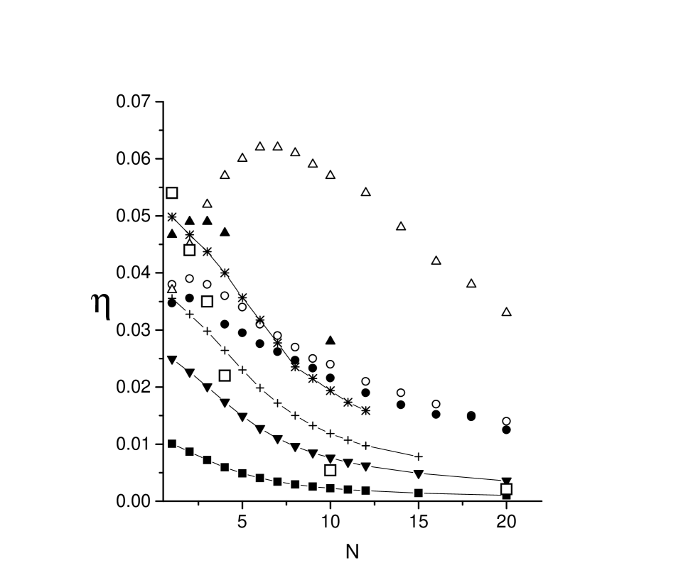
Figure 1: Critical exponent $\eta$ as function of $N$ ($d=3$). Open and full circles represent the standards, they were obtained from the resummation of six (○from [29]) or seven (●from [30]) orders of the perturbation field theory. Recent estimates of [44] from the same perturbative series at order three only are also represented (△). The other estimates are from the exact RG equation expanded up to $O\left(\partial^{2}\right)$ in the derivative expansion: full triangle up from [27], □ from [26]. The points linked by straight lines are from the present work: ■  for $b=0.03$, full triangle down for $b=0.11$, + for $b=0.17011$, * for b=0.25611. See text for discussion.

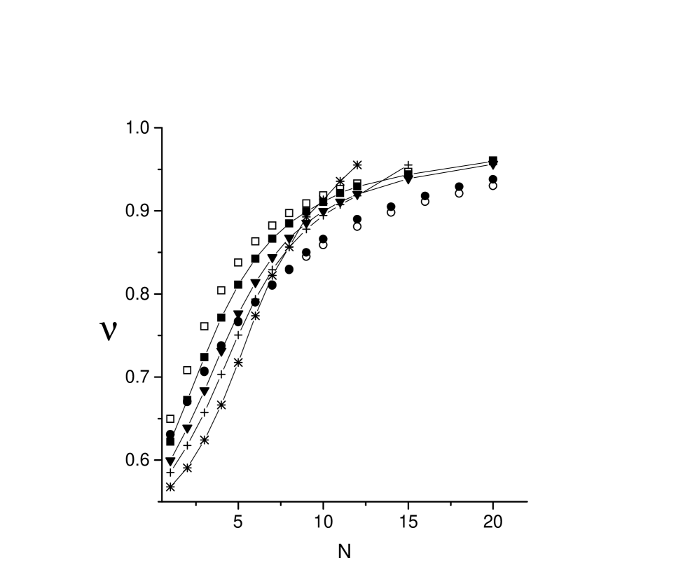
Figure 2: Critical exponent $\nu$ as function of $N$ ($d=3$). Open and full circles represent the standards as in figure 1. The other estimates are from the present work: □  from order LPA, the points linked by straight lines are from $O\left(\partial^{2}\right)$ in the derivative expansion: ■  for $b=0.03$, full triangle down for $b=0.11$, + for $b=0.17011$, * for b=0.25611. See text for discussion.

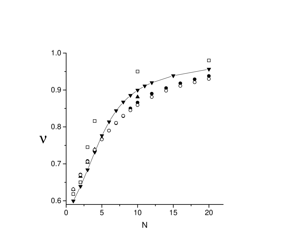
Figure 3: Critical exponent $\nu$ as function of $N$ ($d=3$). Open and full circles represent the standards as in figure 1. The other estimates are from the exact RG equation expanded up to $O\left(\partial^{2}\right)$ in the derivative expansion: full triangle up from [27], □ from [26]. The estimates of the present study for $b=0.11$ is reported (full triangles down linked by straight lines, see figure 2 for the other values of $b$). See text for discussion.

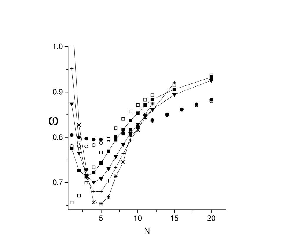
Figure 4: Subcritical exponent $\omega$ as function of $N$ ($d=3$). Open and full circles represent the standards as in figure 1 but the opencircles (○) are from [28]. The other estimates are from the present work: □  from order LPA, the points linked by straight lines are from $O\left(\partial^{2}\right)$ in the derivative expansion: ■  for $b=0.03$, full triangle down for $b=0.11$, + for $b=0.17011$, * for b=0.25611. See text for discussion.

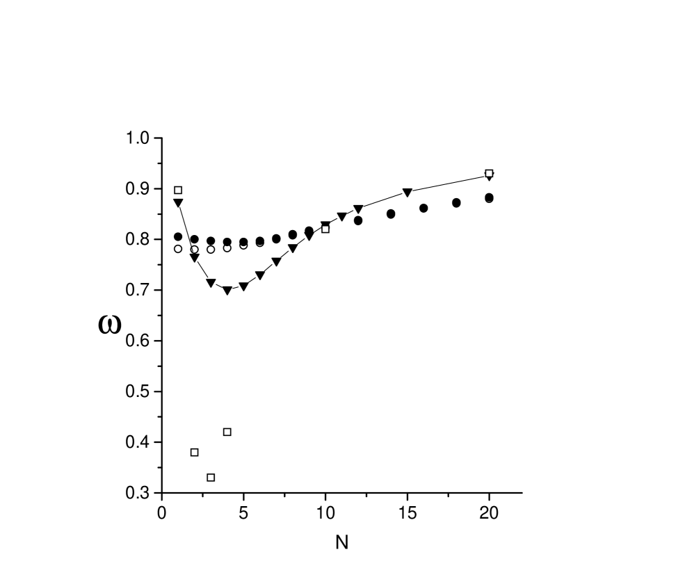
Figure 5: Subcritical exponent $\omega$ as function of $N$ ($d=3$). Open and full circles represent the standards as in figure 4. The other estimates are from the exact RG equation expanded up to $O\left(\partial^{2}\right)$ in the derivative expansion: □ from [26]. The estimates of the present study for $b=0.11$ is reported (full triangles down linked by straight lines, see figure 4 for the other values of $b$). See text for discussion.

References

- [1] Wilson K G and Kogut J 1974 Phys. Rep. 12C 77
- [2] Gell-Mann M and Low F E 1954 Phys. Rev. 95 1300
- [3] Nickel B G, Meiron D I and Baker G A Jr 1977 Compilation of 2-pt and 4-pt graphs for continuous spin models Guelph University preprint unpublished
- [4] Zinn-Justin J 2002 Euclidean Field Theory and Critical Phenomena Fourth edition (Clarendon Press, Oxford)
- [5] Pelissetto A and Vicari E 2002 Phys. Rep. 368 549
- [6] Wilson K G 1976 Phase Transitions and Critical Phenomena Vol. VI ed C. Domb and M.S. Green (Acad. Press, N.-Y.) p 1
- [7] Bagnuls C and Bervillier C 1988 Phys. Rev. Lett. 60 1464
- [8] Delamotte B and Canet L 2004 What can be learnt from the nonperturbative renormalization group? Preprint cond-mat/0412205
- [9] Bagnuls C and Bervillier C 2001 Phys. Rep. 348 91
- [10] Wilson K G 1970 Irvine Conference (unpublished)
- [11] Berges J, Tetradis N and Wetterich C 2002 Phys. Rep. 363 223 Polonyi J 2003 Cent. Eur. J. Phys. 1 1
- [12] Wiese K J 2003 Ann. Inst. Henri Poincaré 4 473 Reuter M and Weyer H 2004 Phys. Rev. D 70 124028 Honerkamp C 2004 Functional renormalization group in the two-dimensional Hubbard model Preprint cond-mat/0411267
- [13] Bervillier C 2004 Phys. Lett. A 332 93
- [14] Bervillier C 2004 Phys. Lett. A 331 110
- [15] Golner G R 1986 Phys. Rev. B 33 7863
- [16] Bagnuls C and Bervillier C 2000 Cond. Matt. Phys. 3 559
- [17] Blaizot J P, Galain R M and Wschebor N 2004 Non Perturbative Renormalization Group, momentum dependence of -point functions and the transition temperature of the weakly interacting Bose gas Preprint cond-mat/0412481
- [18] Tetradis N and Wetterich C 1994 Nucl. Phys. B 422 541
- [19] Bohr O, Schaefer B J and Wambach J 2001 Int. J. Mod. Phys. A 16 3823
- [20] Ballhausen H 2003 The effective average action beyond first order Preprint hep-th/0303070
-
[21]
Ball R D, Haagensen P E, Latorre J I and Moreno E 1995
Phys. Lett. B 347 80
Comellas J 1998 Nucl. Phys. B 509 662 Kubyshin Y, Neves R and Potting R 1999 The Exact Renormalization Group ed A Krasnitz et al (World Scientific, Publ. Co., Singapore) p 159 - [22] Morris T R 1994 Phys. Lett. B 329 241 —–1995 Phys. Lett. B 345 139 Aoki K I, Morikawa K, Souma W, Sumi J I and Terao H 1998 Prog. Theor. Phys. 99 451
- [23] Bonanno A and Zappalà D 2001 Phys. Lett. B 504 181 Mazza M and Zappalà D 2001 Phys. Rev. D 64 105013
- [24] Seide S and Wetterich C 1999 Nucl. Phys. B 562 524 Ballhausen H, Berges J and Wetterich C 2004 Phys. Lett. B 582 144 Canet L 2004 Optimization of field-dependent nonperturbative renormalization group flows Preprint hep-th/0409300
- [25] Canet L, Delamotte B, Mouhanna D and Vidal J 2003 Phys. Rev. B 68 064421
- [26] Morris T R and Turner M D 1998 Nucl. Phys. B 509 637
- [27] Gersdorff G V and Wetterich C 2001 Phys. Rev. B 64 054513
- [28] Sokolov A I 1998, Phys. Status Solidi 40 1169
- [29] Antonenko S A and Sokolov A I 1995 Phys. Rev. E 51 1894
- [30] Kleinert H 1999 Phys. Rev. D 60 085001
- [31] Canet L 2004 Processus de réaction-diffusion : une approche par le groupe de renormalisation non perturbatif Thesis
- [32] Bagnuls C, Bervillier C and Shpot M in progress
- [33] Polchinski J 1984 Nucl. Phys. B 231 269
- [34] Golner G R 1998 Exact renormalization group flow equations for free energies and N-point functions in uniform external fields Preprint hep-th/9801124
- [35] Fisher M E 1983 Critical Phenomena Lecture Notes in Physics ed F.J.W. Hahne (Springer-Verlag, Pub.) p 1
- [36] Bell T L and Wilson K G 1974 Phys. Rev. B 10 3935
- [37] —–1975 Phys. Rev. B 11 3431
- [38] Litim D F 2000 Phys. Lett. B 486 92 —–2001 Phys. Rev. D 64 5007
- [39] Wegner F J 1976 Phase Transitions and Critical Phenomena Vol. VI ed C. Domb and M.S. Green (Acad. Press, N.-Y.) p 7
- [40] Press W H, Flannery B P, Teukolsky S A and Vetterling W T 1986 Numerical Recipes. The Art of Scientific Computing (Cambridge University Press)
- [41] Comellas J and Travesset A 1997 Nucl. Phys. B 498 539
- [42] Litim D F 2001 Int. J. Mod. Phys. A 16 2081
- [43] —–2002 Nucl. Phys. B 631 128
- [44] Kleinert H and Yukalov V I 2004 Self-similar variational perturbation theory for critical exponents Preprint cond-mat/0402163