ITP Budapest Report No. 616
UMTG–245

NLIE for hole excited states in the sine-Gordon model
with two boundaries
Changrim Ahn, Zoltán Bajnok, Rafael I. Nepomechie, László Palla and Gábor Takács²

We derive a nonlinear integral equation (NLIE) for some bulk excited states of the sine-Gordon model on a finite interval with general integrable boundary interactions, including boundary terms proportional to the first time derivative of the field. We use this NLIE to compute numerically the dimensions of these states as a function of scale, and check the UV and IR limits analytically. We also find further support for the ground-state NLIE by comparison with boundary conformal perturbation theory (BCPT), boundary truncated conformal space approach (BTCSA) and the boundary analogue of the Lüscher formula.

1 Introduction

The nonlinear integral equation (NLIE) approach [1, 2] is a powerful tool for studying finite-size effects in the sine-Gordon model with both periodic [2] - [6] and Dirichlet [7, 8] boundary conditions. A NLIE has recently been proposed [9] for the ground state of the sine-Gordon model on a finite interval with more general integrable boundary conditions [10, 11], including new boundary terms proportional to the first time derivative of the field ($\partial_{y}\varphi$). We propose here a NLIE for some bulk excited states of this model, using which we numerically compute the dimensions of these states as a function of scale (the product of the length of the interval and the soliton mass) from ultraviolet (UV) to infrared (IR). We perform checks of the UV and IR limits analytically. Other approaches to studying this model (although without the $\partial_{y}\varphi$ boundary terms) have been considered in [12]-[15].

Our NLIE is based on the Bethe Ansatz solution [16, 17, 18] of the XXZ model with general (both diagonal and nondiagonal) boundary terms [19]. A significant limitation of this solution is that the boundary parameters are not all independent, as they must satisfy a linear constraint relating the left and right boundary parameters. (Such a constraint does not arise in the case of diagonal boundary terms [20, 21, 22].) Consequently, our NLIE is applicable only when the boundary parameters of the sine-Gordon model (including the coefficients of the $\partial_{y}\varphi$ boundary terms) obey a corresponding constraint.

Three different sets of boundary parameters are introduced in the course of this paper: the UV parameters $(\mu_{\pm}\,,\varphi_{0}^{\pm}\,,\kappa_{\pm})$ appearing in the boundary sine-Gordon action; the IR parameters $(\eta_{\pm}\,,\vartheta_{\pm}\,,\gamma_{\pm})$ appearing in the sine-Gordon boundary $S$ matrix; and the lattice parameters $(a_{\pm}\,,b_{\pm}\,,c_{\pm})$ appearing in the XXZ spin-chain Hamiltonian. The relations between the continuum parameters $(\mu_{\pm}\,,\varphi_{0}^{\pm})$ and $(\eta_{\pm}\,,\vartheta_{\pm})$ are known [12, 23]. An important challenge in our Bethe-Ansatz-based approach is to have the correct relations between the lattice and continuum boundary parameters. Such relations were proposed in [9]. The consistency of the results presented here for the UV and IR limits of excited states provides further support for those relations.

The outline of this article is as follows. In Section 2 we collect some results about the sine-Gordon model on a finite interval which we use later to compare with the NLIE results. In particular, we clarify various aspects of the $\partial_{y}\varphi$ boundary terms: the periodicity of the coefficients $\kappa_{\pm}$ (2.11), and the dependence of the UV conformal dimensions (2.29) and of the boundary $S$ matrices (2.37) on these parameters. In Section 3 we review the construction of the counting function for the corresponding light-cone lattice model [9], and the corresponding expression for the Casimir energy (4.11). Moreover, we derive the lattice counting equation (3.16), which is valid also for the homogeneous $(\Lambda=0)$ open XXZ spin chain. In Section 4 we present the continuum NLIE (4.2) which follows from the lattice counting function. For simplicity, we restrict our attention to source contributions from holes and special roots. We also note the relations (4.12), (4.13) between the lattice and continuum boundary parameters, and the constraints (4.14), (4.15) that these parameters must obey. In Section 4.1 we analyze the UV limit. We give the NLIE result for the UV conformal dimensions of states with arbitrary numbers of holes and special roots (4.20), and show that it can be consistent with the CFT result (2.29) for appropriate values of the boundary parameters. In Section 4.2 we analyze the IR limit. In particular, we verify that the IR limit of the NLIE for a one-hole state is equivalent to the Yang equation for a particle on an interval. A noteworthy feature of this computation is that the boundary $S$ matrices [11] which enter the Yang equation are not diagonal. Our numerical results, including comparisons with boundary conformal perturbation theory (BCPT), boundary truncated conformal space approach (BTCSA) [24, 25] and the boundary Lüscher formula [26, 27], are presented in Section 5. Section 6 contains a brief summary and a list of some remaining problems. In Appendix A we present a discussion of BCPT and BTCSA.

2 The sine-Gordon model on a finite interval

In this Section, we collect some results about the sine-Gordon model on a finite interval which will be needed later for making comparisons with NLIE results. In particular, we clarify various aspects of the $\partial_{y}\varphi$ boundary terms: the periodicity of the coefficients $\kappa_{\pm}$, the dependence of the UV conformal dimensions on these parameters, and the dependence of the boundary $S$ matrices on these parameters.

2.1 Action

Following [9], we consider the sine-Gordon quantum field theory on the finite “spatial” interval $x\in\left[x_{-}\,,x_{+}\right]$, with Euclidean action

$${\cal A}_{E}=\int_{-\infty}^{\infty}dy\int_{x_{-}}^{x_{+}}dx\ A(\varphi\,,\partial_{\mu}\varphi)+\int_{-\infty}^{\infty}dy\left[B_{-}(\varphi\,,\partial_{y}\varphi)\Big{|}_{x=x_{-}}+B_{+}(\varphi\,,\partial_{y}\varphi)\Big{|}_{x=x_{+}}\right]\,,$$ (2.1)

where the bulk terms are given by

$$A(\varphi\,,\partial_{\mu}\varphi)={1\over 2}(\partial_{\mu}\varphi)^{2}-\mu_{bulk}\cos(\beta\varphi)\,,$$ (2.2)

and the boundary terms are given by

$$B_{\pm}(\varphi\,,\partial_{y}\varphi)=-\mu_{\pm}\cos({\beta\over 2}(\varphi-\varphi_{0}^{\pm}))\pm i\kappa_{\pm}\partial_{y}\varphi\,.$$ (2.3)

As noted in [9], this action is similar to the one considered by Ghoshal and Zamolodchikov [11], except that now there are two boundaries instead of one, and the boundary action (2.3) contains an additional term depending on the “time” derivative of the field. In the one-boundary case, such a term can be eliminated by adding to the bulk action (2.2) a term proportional to $\partial_{x}\partial_{y}\varphi$, which has no effect on the classical equations of motion. However, in the two-boundary case, one can eliminate in this way only one of the two $\kappa_{\pm}$ parameters (say, $\kappa_{+}$), which results in a shift of the other ($\kappa_{-}\mapsto\kappa_{-}-\kappa_{+}$).

The $\kappa_{\pm}$ parameters are real. The factor of $i$ in the $\partial_{y}\varphi$ terms in (2.3) (which was missed in [9]) is introduced by the Wick rotation from Minkowski to Euclidean space. Indeed, the Minkowski-space action is given by ${\cal A}_{M}=\int_{-\infty}^{\infty}dt\ L_{M}$, with

$$L_{M}=\int_{x_{-}}^{x_{+}}dx\ {1\over 2}\left((\partial_{t}\varphi)^{2}-(\partial_{x}\varphi)^{2}\right)-\kappa_{+}\partial_{t}\varphi(x_{+})+\kappa_{-}\partial_{t}\varphi(x_{-})+\ldots\,,$$ (2.4)

where the ellipsis ($\cdots$) represents the mass terms (proportional to $\mu_{bulk}$ or $\mu_{\pm}$) which we have suppressed for brevity. With $\varphi$ and $\kappa_{\pm}$ real, the Minkowski-space action is real, as is necessary. Rotating to Euclidean space $t=-iy$, $\partial_{t}\varphi=i\partial_{y}\varphi$, we see that

$$L_{M}=-\left\{\int_{x_{-}}^{x_{+}}dx\ {1\over 2}\left((\partial_{y}\varphi)^{2}+(\partial_{x}\varphi)^{2}\right)+i\kappa_{+}\partial_{y}\varphi(x_{+})-i\kappa_{-}\partial_{y}\varphi(x_{-})+\ldots\right\}\equiv-L_{E}\,.$$ (2.5)

Hence, ${\cal A}_{M}=\int_{-\infty}^{\infty}(-idy)\ (-L_{E})=i{\cal A}_{E}$, with the Euclidean action ${\cal A}_{E}=\int_{-\infty}^{\infty}dy\ L_{E}$ given by Eqs. (2.1)-(2.3). As usual, $e^{i{\cal A}_{M}}=e^{-{\cal A}_{E}}$.

An important observation is that the $\kappa_{\pm}$ parameters are periodic, with periodicity $\beta/2$. Indeed, first observe that the action (2.1)-(2.3) has the periodicity

$$\varphi(x,y)\mapsto\varphi(x,y)+{4\pi\over\beta}\,.$$ (2.6)

The contribution from the $\partial_{y}\varphi$ boundary terms to $e^{-{\cal A}_{E}}$ in the Euclidean path integral $\int{\cal D}\varphi\ e^{-{\cal A}_{E}}$ is evidently given by

$$e^{-i\left(\kappa_{+}\Delta\varphi(x_{+})-\kappa_{-}\Delta\varphi(x_{-})\right)}\,,$$ (2.7)

where

$$\Delta\varphi(x)\equiv\int_{-\infty}^{\infty}dy\ \partial_{y}\varphi(x,y)=\varphi(x,y=\infty)-\varphi(x,y=-\infty)\,.$$ (2.8)

Let us compactify the $y$ axis to a circle, so that $y=-\infty$ and $y=\infty$ correspond to the same point. It follows that the sine-Gordon field on the boundary at $y=-\infty$ must be identified with that at $y=\infty$, up to the periodicity (2.6). Hence,

$$\Delta\varphi(x_{\pm})={4\pi\over\beta}n_{\pm}\,,$$ (2.9)

where $n_{\pm}$ are integers. It follows that the contribution (2.7) to $e^{-{\cal A}_{E}}$ becomes

$$e^{-{4\pi i\over\beta}\left(\kappa_{+}n_{+}-\kappa_{-}n_{-}\right)}\,,$$ (2.10)

which has the periodicity

$$\kappa_{\pm}\mapsto\kappa_{\pm}+{\beta\over 2}\,.$$ (2.11)

We recall here that it is useful to introduce the parameters $\lambda$ and $\nu$ which are related to the bulk coupling constant $\beta$,

$$\lambda={8\pi\over\beta^{2}}-1={1\over\nu-1}\,.$$ (2.12)

Hence, the attractive ($0<\beta^{2}<4\pi$) and repulsive ($4\pi<\beta^{2}<8\pi$) regimes correspond to the ranges $1<\nu<2$ and $\nu>2$, respectively.

2.2 Ultraviolet limit

The sine-Gordon model (2.1)-(2.3) can be regarded as a perturbed $c=1$ boundary conformal field theory (CFT). In the ultraviolet limit $\mu_{bulk},\mu_{\pm}\rightarrow 0$, the Minkowski-space Lagrangian is given by (see (2.4))

$$L_{M}=\int_{x_{-}}^{x_{+}}dx\ {1\over 2}\left((\partial_{t}\varphi)^{2}-(\partial_{x}\varphi)^{2}\right)-\kappa_{+}\partial_{t}\varphi(x_{+})+\kappa_{-}\partial_{t}\varphi(x_{-})\,.$$ (2.13)

It follows from the variational principle that $\varphi(x,t)$ obeys the massless free field equation and Neumann boundary conditions,

$$\left(\partial_{t}^{2}-\partial_{x}^{2}\right)\varphi(x,t)=0\,,\qquad\partial_{x}\varphi(x,t)|_{x=x_{\pm}}=0\,.$$ (2.14)

Although the $\partial_{t}\varphi$ boundary terms do not affect the central charge (they are “marginal” perturbations), they modify the expression for the conformal dimension, which we now proceed to compute by canonical quantization.

The canonical momentum $\Pi$ conjugate to $\varphi$ is given by

$$\Pi={\delta{\cal L}\over\delta(\partial_{t}\varphi)}=\partial_{t}\varphi-\kappa_{+}\delta(x-x_{+})+\kappa_{-}\delta(x-x_{-})\,,$$ (2.15)

where ${\cal L}$ is the Lagrange density whose spatial integral is the Lagrangian (2.13). We expand $\varphi$ in terms of modes,

$$\varphi(x,t)=\varphi_{0}+\pi_{0}{t\over L}+{i\over\sqrt{\pi}}\sum_{n\neq 0}{1\over n}\alpha_{n}\cos(\pi n(x-x_{-})/L)e^{-i\pi nt/L}\,,$$ (2.16)

where $L=x_{+}-x_{-}$. One can verify that this expression satisfies the equations of motion (2.14). The mode expansion for $\Pi$ is obtained by substituting (2.16) into (2.15). Note that the momentum zero mode $\Pi_{0}$ is given by

$$\Pi_{0}=\int_{x_{-}}^{x_{+}}dx\ \Pi(x,t)=\pi_{0}-\kappa_{+}+\kappa_{-}\,.$$ (2.17)

The canonical equal-time commutation relations

$$\left[\Pi(x,t)\,,\varphi(x^{\prime},t)\right]=-i\delta(x-x^{\prime})\,,\qquad\left[\Pi(x,t)\,,\Pi(x^{\prime},t)\right]=\left[\varphi(x,t)\,,\varphi(x^{\prime},t)\right]=0\,,$$ (2.18)

imply that $\left[\alpha_{n}\,,\alpha_{m}\right]=n\delta_{n+m,0}$ and

$$\left[\Pi_{0}\,,\varphi_{0}\right]=-i\,.$$ (2.19)

The Hamiltonian is given by

$$H=\int_{x_{-}}^{x_{+}}dx\ {\cal H}\,,\qquad{\cal H}=\Pi\ \partial_{t}\varphi-{\cal L}\,.$$ (2.20)

Substituting the mode expansions, we obtain

$$H={1\over 2L}\pi_{0}^{2}+\mbox{ modes }\,,$$ (2.21)

where “modes” represents the contribution of the oscillators $\alpha_{n}$. The wave functional of the zero mode is a plane wave,

$$\Psi(\varphi_{0})=e^{i\Pi_{0}\varphi_{0}}\,.$$ (2.22)

Let us now compactify the Boson on a circle with radius $r$, which means that the theory is invariant under

$$\varphi(x,t)\mapsto\varphi(x,t)+2\pi r\,,$$ (2.23)

or equivalently, $\varphi_{0}\mapsto\varphi_{0}+2\pi r$. Imposing this condition on the wave functional $\Psi(\varphi_{0})=\Psi(\varphi_{0}+2\pi r)$ implies the quantization of the momentum zero mode,

$$\Pi_{0}={n\over r}\,,$$ (2.24)

where $n$ is an integer. In view of (2.17), (2.21) and (2.24), the zero-mode contribution to the energy is

$$E_{0\,,n}={1\over 2L}\left({n\over r}+\kappa_{+}-\kappa_{-}\right)^{2}\,.$$ (2.25)

Comparing this result with the CFT result

$$E_{0\,,n}=-{\pi\over 24L}(c_{eff}-1)={\pi\over L}\Delta_{n}$$ (2.26)

leads to the following expression for the conformal dimension

$$\Delta_{n}={1\over 2\pi}\left({n\over r}+\kappa_{+}-\kappa_{-}\right)^{2}\,.$$ (2.27)

For the boundary sine-Gordon model and its UV limit, the compactification radius must be

$$r={2\over\beta}\,,$$ (2.28)

corresponding to the periodicity (2.6). We conclude that $\Delta_{n}$ is given by

$$\Delta_{n} = {1\over 2\pi}\left({n\beta\over 2}+\kappa_{+}-\kappa_{-}\right)^{2}$$ (2.29)

$$= {1\over 4\nu(\nu-1)}\left[2n(\nu-1)+{4\over\beta}(\nu-1)(\kappa_{+}-\kappa_{-})\right]^{2}\,.$$

This result is consistent with the $\kappa_{\pm}$ periodicity (2.11). Also, this result is “dual” to the corresponding result for a free massless Boson with Dirichlet boundary conditions [28, 29].

2.3 Boundary $S$ matrices

Results from the theory on the left half line [11] imply that the right and left boundary $S$ matrices $R(\theta\,;\eta_{\pm},\vartheta_{\pm},\gamma_{\pm})$ are given by

$$R(\theta\,;\eta,\vartheta,\gamma)=r_{0}(\theta)\ r_{1}(\theta\,;\eta,\vartheta)\ M(\theta\,;\eta,\vartheta,\gamma)\,,$$ (2.30)

where $M$ has matrix elements

$$M(\theta\,;\eta,\vartheta,\gamma)=\left(\begin{array}[]{cc}m_{11}&m_{12}\\ m_{21}&m_{22}\end{array}\right)\,,$$ (2.33)

where

$$m_{11} = \cos\eta\cosh\vartheta\cosh(\lambda\theta)+i\sin\eta\sinh\vartheta\sinh(\lambda\theta)\,,$$

$$m_{22} = \cos\eta\cosh\vartheta\cosh(\lambda\theta)-i\sin\eta\sinh\vartheta\sinh(\lambda\theta)\,,$$

$$m_{12} = ie^{i\gamma}\sinh(\lambda\theta)\cosh(\lambda\theta)\,,$$

$$m_{21} = ie^{-i\gamma}\sinh(\lambda\theta)\cosh(\lambda\theta)\,.$$ (2.34)

Moreover, the scalar factors have the integral representations (see, e.g., [14])

$$r_{0}(\theta) = \exp\left\{2i\int_{0}^{\infty}{d\omega\over\omega}\sin(2\theta\omega/\pi){\sinh((\nu-2)\omega/2)\sinh(3\omega/2)\over\sinh((\nu-1)\omega/2)\sinh(2\omega)}\right\}\,,$$

$$r_{1}(\theta\,;\eta,\vartheta) = {1\over\cos\eta\cosh\vartheta}\sigma(\eta,\theta)\ \sigma(i\vartheta,\theta)\,,$$ (2.35)

where

$$\sigma(x,\theta)=\exp\left\{2\int_{0}^{\infty}{d\omega\over\omega}\sin((i\pi-\theta)\omega/(2\pi))\sin(\theta\omega/(2\pi)){\cosh((\nu-1)\omega x/\pi)\over\sinh((\nu-1)\omega/2)\cosh(\omega/2)}\right\}\,.$$ (2.36)

Note the presence of the factors $e^{\pm i\gamma}$ in the off-diagonal matrix elements $m_{12}$ and $m_{21}$, which are related to the presence of the $\partial_{y}\varphi$ terms in the boundary action (2.3), and which are absent in the case of a single boundary [11]. In [9] an argument from [11] was borrowed to determine the relation between the (real) parameters $\gamma_{\pm}$ in the boundary $S$ matrix and the (real) parameters $\kappa_{\pm}$ in the boundary action; namely (after correcting for the missing $i$), $\gamma_{\pm}=\beta\kappa_{\pm}/\pi$. However, this relation seems to be incorrect, since it would imply that the factors $e^{i\gamma_{\pm}}$ do not have the periodicity (2.11). We propose here instead the relation

$$\gamma_{\pm}={4\pi\over\beta}\kappa_{\pm}\,,$$ (2.37)

which implies that the factors $e^{i\gamma_{\pm}}$ (and hence, the boundary $S$ matrix) do have the expected periodicity (2.11).

The relation (2.37) for the right boundary can be understood from elementary considerations. Indeed, for the theory on the left half-line $x_{-}=-\infty\,,x_{+}=0$, the Minkowski-space Lagrangian (2.13) can be written in the form

$$L_{M}=L_{M}\left(\kappa_{+}=0\right)-\kappa_{+}\partial_{t}\varphi(x=0)\,.$$ (2.38)

The amplitude for a process can be expressed using a path integral of the form

$$\int\mathcal{D}\varphi\ \exp\left(i\int_{-\infty}^{\infty}dt\ L_{M}\right)=e^{-i\kappa_{+}\Delta\varphi}\int\mathcal{D}\varphi\ \exp\left(i\int_{-\infty}^{\infty}dt\ L_{M}\left(\kappa_{+}=0\right)\right)\,,$$ (2.39)

where now

$$\Delta\varphi=\varphi(x=0,\,t=\infty)-\varphi(x=0,\,t=-\infty)\,,$$ (2.40)

with appropriate initial and final configurations of the field $\varphi$ at $t=\mp\infty$. For definiteness, we can fix the asymptotic condition $\varphi(x=-\infty)=0$. For a process involving a soliton reflecting back into a soliton, we have

$$\varphi\left(x=0,t=\mp\infty\right)=\frac{2\pi}{\beta}\qquad\Rightarrow\qquad\Delta\varphi=0\,.$$ (2.41)

Hence, for such processes the amplitude is independent of $\kappa_{+}$; and this is also true for the reflection of an antisoliton into an antisoliton. For a soliton reflecting into an antisoliton we have

$$\varphi\left(x=0,t=\mp\infty\right)=\pm\frac{2\pi}{\beta}\qquad\Rightarrow\qquad\Delta\varphi=-\frac{4\pi}{\beta}\,,$$ (2.42)

which results in a phase factor

$$\exp\left(i\frac{4\pi}{\beta}\kappa_{+}\right)\,.$$ (2.43)

For an antisoliton reflecting into a soliton the resulting phase factor is the inverse of the above. This leads to the relation (2.37) between the parameters in the Lagrangian and the reflection factor for the right boundary.

Similarly, for the left boundary, we consider the theory on the right half-line $x_{-}=0\,,x_{+}=\infty$. The corresponding Lagrangian and path integral are given by (2.38) and (2.39) with $\kappa_{+}\mapsto-\kappa_{-}$; and we now fix $\varphi(x=\infty)=0$. For a soliton reflecting into an antisoliton we have

$$\varphi\left(x=0,t=\mp\infty\right)=\mp\frac{2\pi}{\beta}\qquad\Rightarrow\qquad\Delta\varphi=\frac{4\pi}{\beta}\,,$$ (2.44)

which results in a phase factor

$$\exp\left(i\frac{4\pi}{\beta}\kappa_{-}\right)\,,$$ (2.45)

and leads to the relation (2.37) for the left boundary.

We find further support for relation (2.37) from a study of the UV and IR limits of the NLIE in Sections 4.1 and 4.2.

The relation of the boundary $S$-matrix parameters $\eta_{\pm},\vartheta_{\pm}$ to the parameters $\mu_{\pm}\,,\varphi_{0}^{\pm}$ in the boundary action (2.3) is given by [12, 23]

$$\cos\left({\beta^{2}\over 8\pi}(\eta_{\pm}+i\vartheta_{\pm})\right) = {\mu_{\pm}\over\mu_{c}}e^{\mp{i\over 2}\beta\varphi_{0}^{\pm}}\,,$$

$$\cos\left({\beta^{2}\over 8\pi}(\eta_{\pm}-i\vartheta_{\pm})\right) = {\mu_{\pm}\over\mu_{c}}e^{\pm{i\over 2}\beta\varphi_{0}^{\pm}}\,,$$ (2.46)

where

$$\mu_{c}=\sqrt{2\mu_{bulk}\over\sin\left({\beta^{2}\over 8}\right)}\,.$$ (2.47)

Note that we have introduced an additional minus sign on one of the boundaries. That is, the UV-IR relation is different on the two boundaries, the difference being in the sign of $\varphi_{0}$. The two sets of boundary parameters $(\mu_{\pm}\,,\varphi_{0}^{\pm}\,,\kappa_{\pm})$ and $(\eta_{\pm}\,,\vartheta_{\pm}\,,\gamma_{\pm})$ can be regarded as “UV” and “IR” boundary parameters, respectively; hence, the relations (2.37), (2.46), (2.47) correspond to UV-IR relations.

3 The lattice counting function

The light-cone lattice [30, 31, 32] version of the sine-Gordon model is similar to the XXZ spin chain, the main difference being the introduction of an alternating inhomogeneity parameter $\pm\Lambda$. The solution [16, 17] leads to the Bethe Ansatz equations [9]

$$h^{(+)}(\lambda_{j})=I_{j}^{(+)}\,,\qquad j=1\,,\ldots\,,M^{(+)}\,,$$ (3.1)

where $\{I_{j}^{(+)}\}$ are integers, and the lattice counting function $h^{(+)}(\lambda)$ is given by

$$h^{(+)}(\lambda) = {1\over 2\pi}\Big{\{}N\left[q_{1}(\lambda+\Lambda)+q_{1}(\lambda-\Lambda)\right]+q_{1}(\lambda)+r_{1}(\lambda)+q_{2a_{-}-1}(\lambda)-r_{1+2ib_{-}}(\lambda)$$ (3.2)

$$+ q_{2a_{+}-1}(\lambda)-r_{1+2ib_{+}}(\lambda)-\sum_{k=1}^{M^{(+)}}\left[q_{2}(\lambda-\lambda_{k})+q_{2}(\lambda+\lambda_{k})\right]\Big{\}}\,.$$

The functions $q_{n}(\lambda)$ and $r_{n}(\lambda)$ are odd, and are defined by

$$q_{n}(\lambda) = \pi+i\ln{\sinh\left({\pi\over\nu}(\lambda+{in\over 2})\right)\over\sinh\left({\pi\over\nu}(\lambda-{in\over 2})\right)}=2\tan^{-1}\left(\cot(n\pi/(2\nu))\tanh(\pi\lambda/\nu)\right)\,,$$

$$r_{n}(\lambda) = i\ln{\cosh\left({\pi\over\nu}(\lambda+{in\over 2})\right)\over\cosh\left({\pi\over\nu}(\lambda-{in\over 2})\right)}\,.$$ (3.3)

The real lattice boundary parameters $a_{\pm},b_{\pm},c_{\pm}$ must satisfy the constraints

$$a_{-}+a_{+} = \pm|c_{-}-c_{+}|+k\,,$$

$$b_{-}+b_{+} = 0\,,$$ (3.4)

where the integer $k\in[-(N+1)\,,N+1]$ is even if $N$ is odd, and is odd if $N$ is even. The parameters $a_{\pm}$ can be restricted to the fundamental domain $|2a_{\pm}-1|<2\nu$. The number $M^{(+)}$ of Bethe roots is given by

$$M^{(+)}={1\over 2}(N-1+k)\,,$$ (3.5)

where $k$ is the integer in the constraint (3.4).

The corresponding energy is given by [7, 32]

$$E=-{1\over\delta}\sum_{j=1}^{M^{(+)}}\left[a_{1}(\lambda_{j}+\Lambda)+a_{1}(\lambda_{j}-\Lambda)\right]\,,$$ (3.6)

where $\delta$ is the lattice spacing, and

$$a_{n}(\lambda)={1\over 2\pi}{d\over d\lambda}q_{n}(\lambda)={1\over\nu}{\sin(n\pi/\nu)\over\cosh(2\pi\lambda/\nu)-\cos(n\pi/\nu)}\,.$$ (3.7)

For given values of the bulk and boundary parameters, the counting function $h^{(+)}(\lambda)$ does not give all $2^{N}$ energy levels. The remaining levels can be obtained from a corresponding counting function $h^{(-)}(\lambda)$ with the boundary parameters negated,

$$(a_{\pm}\,,b_{\pm})\mapsto(-a_{\pm}\,,-b_{\pm})\,,$$ (3.8)

and with the number of Bethe roots equal to $M^{(-)}={1\over 2}(N-1-k)$ [18]. We shall refer to this other counting function as the “negated” counting function. Although below we generally explicitly discuss only $h^{(+)}(\lambda)$, corresponding results hold also for $h^{(-)}(\lambda)$.

Since the counting function (3.2) is odd and has the periodicity $\lambda\mapsto\lambda+i\nu$, we can restrict the Bethe roots $\lambda_{j}$ to the following region of the complex $\lambda$ plane [8]

$$\left\{\Re e\ \lambda>0\,,\quad-{\nu\over 2}<\Im m\ \lambda\leq{\nu\over 2}\right\}\bigcup\left\{\Re e\ \lambda=0\,,\quad 0<\Im m\ \lambda<{\nu\over 2}\right\}\,.$$ (3.9)

The origin ($\lambda=0$) is excluded since the corresponding Bethe state would vanish.

The summation over all the roots in the counting function involves the function $q_{2}(\lambda)$, whose fundamental analyticity strip is $|\Im m\ \lambda|<\min(1\,,\nu-1)$. Hence, it is useful to classify the Bethe roots $\lambda_{j}$ in the region (3.9) as either real, “close” ($0<|\Im m\ \lambda_{j}|<\min(1\,,\nu-1)$), or “wide” ($\min(1\,,\nu-1)<|\Im m\ \lambda_{j}|<{\nu\over 2}$). Real solutions of $h^{(+)}(\lambda)=\mbox{ integer }$ which are not Bethe roots are called “holes”. If an “object” (either a root or a hole) has rapidity $\lambda_{j}$ for which the counting function is decreasing (${d\over d\lambda}h^{(+)}(\lambda_{j})<0$), then the object is called “special”. We denote by $M_{R}$, $M_{C}$, $M_{W}$, $N_{H}$ and $N_{S}$ the number of real roots, close roots, wide roots, holes, and special objects, respectively. Note also that $h^{(+)}(\lambda)$ is continuous on the real $\lambda$ axis. For further discussion about general properties of the counting function and the classification of roots and holes, see e.g. [4, 8].

We now proceed to derive a so-called lattice counting equation, which relates $M_{C}$, $M_{W}$, $N_{H}$ and $N_{S}$ (but which is independent of $M_{R}$ and $N$) for any Bethe state. To this end, we first compute the asymptotic limit of the counting function, and take its integer part,

$$\lfloor h^{(+)}(\infty)\rfloor=M^{(+)}+1+{1\over 2}(s_{+}+s_{-})-k+\mathop{\rm sgn}\nolimits(\nu-2)M_{W}+\lfloor{1\over 2}-{1\over\nu}\left(a_{+}+a_{-}-k\right)\rfloor\,,$$ (3.10)

where $\lfloor\quad\rfloor$ denotes integer part, and $s_{\pm}=\mathop{\rm sgn}\nolimits(a_{\pm}-{1\over 2})$, where the sign function $\mathop{\rm sgn}\nolimits(n)$ is defined as

$$\mathop{\rm sgn}\nolimits(n)=\left\{\begin{array}[]{c@{\quad: \quad} l}{n\over|n|}&n\neq 0\\ 0&n=0\end{array}\right.\,.$$ (3.13)

In obtaining the result (3.10), we have used the facts

$$q_{n}(\infty) = \mathop{\rm sgn}\nolimits(n)\pi-{n\pi\over\nu}\quad\mbox{ for }0<|n|<2\nu\,,$$

$$r_{n}(\infty) = -{n\pi\over\nu}\,,$$ (3.14)

as well as the relation (3.5) to eliminate $N$, and the second constraint in (3.4). On the other hand, one can argue that (see e.g. [4])

$$\lfloor h^{(+)}(\infty)\rfloor=N_{H}+M_{R}-2N_{S}\,.$$ (3.15)

Using the evident relation $M^{(+)}=M_{R}+M_{C}+M_{W}$ to eliminate $M_{R}$ on the RHS of (3.15), and then combining with (3.10), we finally obtain the lattice counting equation,

$$N_{H}-2N_{S}=M_{C}+2M_{W}\mbox{step}(\nu-2)+1+{1\over 2}(s_{+}+s_{-})-k+\lfloor{1\over 2}-{1\over\nu}\left(a_{+}+a_{-}-k\right)\rfloor\,,$$ (3.16)

where the step function $\mbox{step}(n)$ is defined as

$$\mbox{step}(n)=\left\{\begin{array}[]{c@{\quad: \quad} l}1&n\geq 0\\ 0&n<0\end{array}\right.\,.$$ (3.19)

The lattice counting equation (3.16) is valid also for the homogeneous $(\Lambda=0)$ open XXZ spin chain.

As a simple example of the utility of this result, consider (as in [9]) the case that $N$ is even with $k=1$, and look for purely real solutions with no holes or special roots $(M_{C}=M_{W}=N_{H}=N_{S}=0)$. The lattice counting equation implies

$$0={1\over 2}(s_{+}+s_{-})+\lfloor{1\over 2}-{1\over\nu}\left(a_{+}+a_{-}-1\right)\rfloor\,,$$ (3.20)

which is a condition on the boundary parameters $a_{\pm}$ that is necessary for such solutions to exist. Numerical checks suggest that this might also be a sufficient condition for the existence of such solutions.

4 Nonlinear integral equation

The lattice NLIE can be derived from the lattice counting function (3.2) by standard manipulations [2] - [8]. The continuum limit consists of taking the number of spins $N\rightarrow\infty$, the lattice spacing $\delta\rightarrow 0$, and the inhomogeneity parameter $\Lambda\rightarrow\infty$, in such a way that the length $L=x_{+}-x_{-}$ and the soliton mass $m$ (whose relation to $\mu_{bulk}$ is given by (A.12)) are given by

$$L=N\delta\,,\qquad m={2\over\delta}e^{-\pi\Lambda}\,,$$ (4.1)

respectively. Changing to the rescaled rapidity variable $\theta=\pi\lambda$, and setting $f^{(+)}(\theta)=2\pi ih^{(+)}(\theta)$, one arrives at the continuum NLIE for $f^{(+)}(\theta)$

$$f^{(+)}(\theta) = 2imL\sinh\theta+iP_{bdry}^{(+)}(\theta)+ig(\theta)$$ (4.2)

$$+ {2i\over\pi}\int_{-\infty}^{\infty}d\theta^{\prime}\ \Im m\ G(\theta-\theta^{\prime}-i\epsilon)\ \ln(1-e^{f^{(+)}(\theta^{\prime}+i\epsilon)})\,,$$

where $G(\theta)$ is given by

$$G(\theta)={1\over 2\pi}\int_{-\infty}^{\infty}d\omega\ e^{-i\omega\theta/\pi}\hat{G}(\omega)\,,$$ (4.3)

and the Fourier transform $\hat{G}(\omega)$ is given by

$$\hat{G}(\omega)={\sinh((\nu-2)\omega/2)\over 2\sinh((\nu-1)\omega/2)\cosh(\omega/2)}\,.$$ (4.4)

Furthermore, $P_{bdry}^{(+)}(\theta)$ is the odd function satisfying ${P_{bdry}^{(+)}}^{\prime}(\theta)=2R^{(+)}(\theta)$, where $R^{(+)}(\theta)$ is given (as in (4.3)) in terms of its Fourier transform

$$\hat{R}^{(+)}(\omega)={\sinh((\nu-2)\omega/4)\cosh(\nu\omega/4)\over\sinh((\nu-1)\omega/2)\cosh(\omega/2)}+{\sinh((\nu-2)\omega/2)\over 2\sinh((\nu-1)\omega/2)\cosh(\omega/2)}$$

$$+{s_{+}\sinh((\nu-|2a_{+}-1|)\omega/2)\over 2\sinh((\nu-1)\omega/2)\cosh(\omega/2)}+{\sinh((1+2ib_{+})\omega/2)\over 2\sinh((\nu-1)\omega/2)\cosh(\omega/2)}+(+\leftrightarrow-)\,,$$

where $(+\leftrightarrow-)$ is a shorthand for two additional terms which are the same as those on the second line of (4), but with $a_{+},s_{+}$ and $b_{+}$ replaced by $a_{-},s_{-}$ and $b_{-}$, respectively.

Moreover, $g(\theta)$ is the source term. For simplicity, we henceforth restrict our attention to source contributions from holes and special roots; other bulk sources (close or wide roots) can presumably be treated in the same manner as in [4, 8]. The source term is therefore given by

$$g(\theta) = \sum_{j=1}^{N_{H}}\left[\chi(\theta-\theta_{j}^{H})+\chi(\theta+\theta_{j}^{H})\right]$$

$$- \sum_{j=1}^{N_{S}}\left[\chi(\theta-\theta_{j}^{S}+i\epsilon)+\chi(\theta-\theta_{j}^{S}-i\epsilon)+\chi(\theta+\theta_{j}^{S}+i\epsilon)+\chi(\theta+\theta_{j}^{S}-i\epsilon)\right]\,,$$

where $\chi(\theta)$ is the odd function satisfying $\chi^{\prime}(\theta)=2G(\theta)$, the latter function being given by (4.3). Finally, $\theta_{j}^{H}$ and $\theta_{j}^{S}$ are the positions of the holes and special roots, respectively, whose corresponding distinct, positive integers we label by $I_{j}^{H}$ and $I_{j}^{S}$,

$$f^{(+)}(\theta_{j}^{H})=2\pi iI_{j}^{H}\,,\qquad f^{(+)}(\theta_{j}^{S})=2\pi iI_{j}^{S}\,.$$ (4.7)

For the continuum model, the value $I_{j}=0$ is excluded because the corresponding rapidity $\theta_{j}=0$ is not physical.

The energy is given by

$$E=\epsilon_{bulk}L+\epsilon_{boundary}+E_{Casimir}\,,$$ (4.8)

where $\epsilon_{bulk}$ and $\epsilon_{boundary}$ are given by [9]

$$\epsilon_{bulk}={1\over 4}m^{2}\cot(\nu\pi/2)$$ (4.9)

and

$$\epsilon_{boundary}=-{m\over 2}\left[-\cot(\nu\pi/4)-1+{\cos((\nu-2s_{+}a_{+})\pi/2)\over\sin(\nu\pi/2)}+{\cosh(\pi b_{+})\over\sin(\nu\pi/2)}+(+\leftrightarrow-)\right]\,,$$ (4.10)

and $E_{Casimir}$ (order $1/L$) is given by

$$E_{Casimir} = m\sum_{j=1}^{N_{H}}\cosh\theta_{j}^{H}-m\sum_{j=1}^{N_{S}}\left[\cosh(\theta_{j}^{S}+i\epsilon)+\cosh(\theta_{j}^{S}-i\epsilon)\right]$$ (4.11)

$$- {m\over 2\pi}\int_{-\infty}^{\infty}d\theta\ \Im m\ \sinh(\theta+i\epsilon)\ln(1-e^{f^{(+)}(\theta+i\epsilon)})\,.$$

The following relations between the continuum IR ($\eta_{\pm}\,,\vartheta_{\pm}$) and lattice ($a_{\pm}\,,b_{\pm}$) boundary parameters were obtained in [9]

$$\eta_{\pm} = \mp{\pi(s_{\pm}\nu-2a_{\pm})\over 2(\nu-1)}\,,$$

$$\vartheta_{\pm} = {\pi b_{\pm}\over\nu-1}\,.$$ (4.12)

These relations were obtained by comparing the continuum [12, 23] and lattice expressions for the boundary energy. A relation between $\gamma_{\pm}$ and $c_{\pm}$ was also conjectured in [9]

$$\gamma_{\pm}={\pi c_{\pm}\over\nu-1}\,,$$ (4.13)

for which we shall find further support from analysis of the UV and IR limits in Sections 4.1 and 4.2 below. Note that these relations together with the constraints (3.4) among the lattice boundary parameters imply corresponding constraints among the continuum IR boundary parameters,

$$\eta_{-}-\eta_{+} = \mp|\gamma_{-}-\gamma_{+}|+{\pi\over\nu-1}\left[{1\over 2}(s_{+}+s_{-})\nu-k\right]\,,$$

$$\vartheta_{-}+\vartheta_{+} = 0\,.$$ (4.14)

The UV and IR limits also imply that, in the continuum limit, the integer $k$ must be restricted to odd values,

$$k=\mbox{ odd }\,.$$ (4.15)

The UV-IR relations (2.37), (2.46), (2.47) imply corresponding constraints among the UV parameters appearing in the boundary sine-Gordon action. We emphasize that our NLIE describes the sine-Gordon model only for values of boundary parameters which satisfy these constraints.

It is interesting to consider the continuum version of the lattice counting equation (3.16). For the case of periodic boundary conditions, Destri and de Vega have argued [4] that the continuum result coincides with the lattice result without the integer part term. It is therefore plausible that for the case at hand the continuum counting equation is given by

$$N_{H}-2N_{S}=M_{C}+2M_{W}\mbox{step}(\nu-2)+1+{1\over 2}(s_{+}+s_{-})-k\,.$$ (4.16)

We shall find some support for this conjecture when we consider the UV limit below.

4.1 Ultraviolet limit

We now consider the UV limit $mL\rightarrow 0$. In this limit, only large values of $|\theta|$ contribute to the Casimir energy. Indeed, the driving term of the NLIE implies that one must consider the scaling limit

$$\theta=\ln{1\over mL}+\tilde{\theta}\,,$$ (4.17)

where $\tilde{\theta}$ is finite as $mL\rightarrow 0$. Hence, one must distinguish whether the positions of the sources remain finite or scale in the same manner. Let $N_{H}^{0}$ ($N_{H}^{\infty}$) be the number of holes whose positions $\theta_{j}^{H\ 0}$ ($\theta_{j}^{H\ \infty}$) remain finite (scale), with corresponding integers $I_{j}^{H\ 0}$ ($I_{j}^{H\ \infty}$, respectively); and similarly for the special roots. Hence,

$$\theta_{j}^{H\ \infty}=\ln{1\over mL}+\tilde{\theta}_{j}^{H\ \infty}\,,\qquad\theta_{j}^{S\ \infty}=\ln{1\over mL}+\tilde{\theta}_{j}^{S\ \infty}\,,$$ (4.18)

with $\tilde{\theta}_{j}^{H\ \infty}$ and $\tilde{\theta}_{j}^{S\ \infty}$ finite as $mL\rightarrow 0$, and

$$N_{H}=N_{H}^{0}+N_{H}^{\infty}\,,\qquad N_{S}=N_{S}^{0}+N_{S}^{\infty}\,.$$ (4.19)

Proceeding to compute the Casimir energy from (4.2) and (4.11) as in [4]-[7], imposing the constraints (3.4), and recalling that $E_{Casimir}=-{c_{eff}\pi\over 24L}$ with $c_{eff}=1-24\Delta_{n}$, we obtain

$$\Delta_{n} = {1\over 4\nu(\nu-1)}\Bigg{\{}\nu\left[{1\over 2}(s_{+}+s_{-})+N_{H}^{0}-N_{H}^{\infty}-2N_{S}^{0}+2N_{S}^{\infty}\right]-\left(k-1+2N_{H}^{0}-4N_{S}^{0}\right)$$ (4.20)

$$\mp |c_{-}-c_{+}|\Bigg{\}}^{2}+\sum_{j=1}^{N_{H}^{\infty}}I_{j}^{H\ \infty}-2\sum_{j=1}^{N_{S}^{\infty}}I_{j}^{S\ \infty}-{1\over 2}(N_{H}^{\infty}-2N_{S}^{\infty})(N_{H}^{\infty}-2N_{S}^{\infty}+1)\,.$$

The result (4.20) for the conformal dimension is consistent with the CFT result (2.29) if we identify

$$c_{\pm}={4\over\beta}(\nu-1)\kappa_{\pm}\,,$$ (4.21)

and set

$${1\over 2}(s_{+}+s_{-})+N_{H}^{0}-N_{H}^{\infty}-2N_{S}^{0}+2N_{S}^{\infty}=k-1+2N_{H}^{0}-4N_{S}^{0}=2n\,,$$ (4.22)

where $n$ is an integer. The relation (4.21) together with (2.37) implies the relation (4.13) between the boundary parameters $\gamma_{\pm}$ and $c_{\pm}$. Note that the result (4.20) for the conformal dimension contains not only the contribution (2.29) corresponding to the highest weights, but also additional integer-valued terms corresponding to their descendants.

It follows from (4.19) and (4.22) that

$$N_{H}-2N_{S}=1+{1\over 2}(s_{+}+s_{-})-k\,,$$ (4.23)

which is in agreement with the conjectured continuum counting equation (4.16) for the special case $M_{C}=M_{W}=0$ that we are considering. Moreover, (4.22) implies the result (4.15) that $k$ must be an odd integer.

Here are three examples:

Ex. 1

A Bethe state consisting of only real roots and no holes or special roots ($N_{H}=N_{S}=0$) with $k=1$ has, according to (4.23), a “good” UV limit only if the boundary parameters satisfy $s_{+}+s_{-}=0$; and its UV dimension, according to (4.22), is given by (2.29) with $n=0$.

Ex. 2

A Bethe state consisting of only real roots and 1 hole and no special roots ($N_{H}=1\,,N_{S}=0$) with $k=1$ has a “good” UV limit only if $s_{+}+s_{-}=2$. Its UV dimension is given by (2.29) with either $n=1$ or $n=0$, depending on whether in the UV limit the hole’s rapidity remains finite ($N_{H}^{0}=1\,,N_{H}^{\infty}=0$) or infinite ($N_{H}^{0}=0\,,N_{H}^{\infty}=1$), respectively.

Ex. 3

For $k=-1$, it is possible to have a Bethe state with a “good” UV limit consisting of only real roots and 2 holes and no special roots ($N_{H}=2\,,N_{S}=0$), provided $s_{+}+s_{-}=0$. Its UV dimension is given by (2.29) with $n$ values equal to either $1\,,0\,,$ or $-1$ depending on whether in the UV limit the hole rapidities are either both finite, one finite and one infinite, or both infinite, respectively.

4.2 Infrared limit

We verify in this Section that the IR limit of the NLIE for a one-hole state is equivalent to the Yang equation for a particle on an interval. Indeed, in the IR limit $mL\rightarrow\infty$, the integral terms in the NLIE (4.2) and in the energy formula (4.11) are of order $O(e^{-mL})$ and can therefore be neglected. For a single hole with rapidity $\theta_{H}$, the NLIE becomes

$$f^{(+)}(\theta)=2imL\sinh\theta+iP_{bdry}^{(+)}(\theta)+i\chi(\theta-\theta_{H})+i\chi(\theta+\theta_{H})\,.$$ (4.24)

Noting that $e^{f^{(+)}(\theta_{H})}=1$ on account of Eq. (4.7), we obtain the following relation for $\theta_{H}$

$$e^{2imL\sinh\theta_{H}}e^{i\left(P_{bdry}^{(+)}(\theta_{H})+\chi(2\theta_{H})\right)}=1\,.$$ (4.25)

A similar relation can be derived from the negated counting function,

$$e^{2imL\sinh\theta_{H}}e^{i\left(P_{bdry}^{(-)}(\theta_{H})+\chi(2\theta_{H})\right)}=1\,,$$ (4.26)

where $P_{bdry}^{(-)}(\theta)$ differs from $P_{bdry}^{(+)}(\theta)$ by the negation of the boundary parameters (3.8). These relations should be equivalent to the Yang equation for a particle on an interval of length $L$,

$$e^{2imL\sinh\theta_{H}}R(\theta_{H}\,;\eta_{+},\vartheta_{+},\gamma_{+})R(\theta_{H}\,;\eta_{-},\vartheta_{-},\gamma_{-})|\theta_{H},(\pm)\rangle=|\theta_{H},(\pm)\rangle\,,$$ (4.27)

where the boundary $S$ matrices $R(\theta\,;\eta_{\pm},\vartheta_{\pm},\gamma_{\pm})$ are given by (2.30), and $|\theta_{H},(\pm)\rangle$ denote the two possible one-particle states.

In other words, dropping the subscript $H$ of the hole rapidity, the expressions $e^{i\left(P_{bdry}^{(\pm)}(\theta)+\chi(2\theta)\right)}$ should be equal to the two eigenvalues of the Yang matrix $Y(\theta)$, which is defined by

$$Y(\theta)=R(\theta\,;\eta_{+},\vartheta_{+},\gamma_{+})R(\theta\,;\eta_{-},\vartheta_{-},\gamma_{-})\,.$$ (4.28)

Indeed, for a state with real roots and one hole, Eq. (4.16) implies that $k={1\over 2}(s_{+}+s_{-})$. Since $k$ must be odd, it follows that the only two possibilities are $k=s_{\pm}=1$ or $k=s_{\pm}=-1$. For definiteness, we consider the former case, $k=s_{\pm}=1$, and therefore, ${1\over 2}<a_{\pm}<{1\over 2}+\nu$. From the definitions of $P_{bdry}^{(\pm)}(\theta)$ and $\chi(\theta)$, it follows that

$$P_{bdry}^{(\pm)}(\theta)+\chi(2\theta)=2\int_{0}^{\infty}{d\omega\over\omega}\left[\sin(\omega\theta/\pi)\hat{R}^{(\pm)}(\omega)+\sin(2\omega\theta/\pi)\hat{G}(\omega)\right]\,.$$ (4.29)

With the help of the expression (4) for $\hat{R}^{(+)}(\omega)$ (and a similar expression with the boundary parameters negated (3.8) for $\hat{R}^{(-)}(\omega)$) and the identity [34]

$${\sinh((\nu-2)\omega/4)\cosh(\nu\omega/4)\over\sinh((\nu-1)\omega/2)\cosh(\omega/2)}+{\sinh((\nu-2)\omega/2)\over 2\sinh((\nu-1)\omega/2)\cosh(\omega/2)}$$ (4.30)

$$={2\sinh((\nu-2)\omega/4)\sinh(3\omega/4)\over\sinh((\nu-1)\omega/4)\sinh\omega}-\hat{G}(\omega/2)\,,$$

we obtain

$$e^{i\left(P_{bdry}^{(\pm)}(\theta)+\chi(2\theta)\right)} = \exp 2i\int_{0}^{\infty}{d\omega\over\omega}\sin(2\omega\theta/\pi)\Big{\{}{2\sinh((\nu-2)\omega/2)\sinh(3\omega/2)\over\sinh((\nu-1)\omega/2)\sinh(2\omega)}$$

$$+ {\sinh((1\pm(\nu-2a_{+}))\omega)\over 2\sinh((\nu-1)\omega)\cosh\omega}+{\sinh((1\pm 2ib_{+})\omega)\over 2\sinh((\nu-1)\omega)\cosh\omega}+(+\leftrightarrow-)\Big{\}}\,.$$

Finally, using the relations (4.12) between the lattice and continuum IR boundary parameters, we obtain

$$e^{i\left(P_{bdry}^{(\pm)}(\theta)+\chi(2\theta)\right)} = \exp 2i\int_{0}^{\infty}{d\omega\over\omega}\sin(2\omega\theta/\pi)\Big{\{}{2\sinh((\nu-2)\omega/2)\sinh(3\omega/2)\over\sinh((\nu-1)\omega/2)\sinh(2\omega)}$$

$$+ {\sinh((1\mp(\nu-1)2\eta_{+}/\pi)\omega)\over 2\sinh((\nu-1)\omega)\cosh\omega}+{\sinh((1\pm(\nu-1)2\eta_{-}/\pi)\omega)\over 2\sinh((\nu-1)\omega)\cosh\omega}$$

$$+ {\sinh((1\pm(\nu-1)2i\vartheta_{+}/\pi)\omega)\over 2\sinh((\nu-1)\omega)\cosh\omega}+{\sinh((1\pm(\nu-1)2i\vartheta_{-}/\pi)\omega)\over 2\sinh((\nu-1)\omega)\cosh\omega}\Big{\}}\,.$$

We now turn to the computation of the eigenvalues of the Yang matrix (4.28). Recalling (2.30), we see that the eigenvalues $y^{(\pm)}$ of $Y(\theta)$ are given by

$$y^{(\pm)}=r_{0}(\theta)^{2}r_{1}(\theta\,;\eta_{+},\vartheta_{+})r_{1}(\theta\,;\eta_{-},\vartheta_{-})\Lambda^{(\pm)}\,,$$ (4.33)

where $\Lambda^{(\pm)}$ denote the eigenvalues of $M(\theta\,;\eta_{+},\vartheta_{+},\gamma_{+})M(\theta\,;\eta_{-},\vartheta_{-},\gamma_{-})$. Although the expressions for $\Lambda^{(\pm)}$ are generally very complicated, a remarkable simplification occurs if the boundary parameters satisfy the constraints (4.14), (4.15). Indeed, in that case, the eigenvalues are factorizable into a product of trigonometric functions,

$$\Lambda^{(\pm)}=\cos(-\eta_{+}\mp i\lambda\theta)\cos(\eta_{-}\mp i\lambda\theta)\cos(i\vartheta_{+}\mp i\lambda\theta)\cos(i\vartheta_{-}\mp i\lambda\theta)\,.$$ (4.34)

Recalling the expressions (2.35) for $r_{0}(\theta)$ and $r_{1}(\theta\,;\eta,\vartheta)$, using the identity

$${1\over\cos x}\cos(x\mp i\lambda\theta)\ \sigma(x,\theta)=\exp\left\{2i\int_{0}^{\infty}{d\omega\over\omega}\sin(2\theta\omega/\pi){\sinh((1\pm(\nu-1)2x/\pi)\omega)\over 2\sinh((\nu-1)\omega)\cosh\omega}\right\}\,,$$ (4.35)

and comparing with (4.2), we obtain the desired result

$$e^{i\left(P_{bdry}^{(\pm)}(\theta)+\chi(2\theta)\right)}=r_{0}(\theta)^{2}r_{1}(\theta\,;\eta_{+},\vartheta_{+})r_{1}(\theta\,;\eta_{-},\vartheta_{-})\Lambda^{(\pm)}=y^{(\pm)}\,.$$ (4.36)

That is, we have verified that the IR limit of the NLIE for a one-hole state is equivalent to the Yang equation for a particle on an interval. We stress that the boundary $S$ matrices entering the Yang equation are not diagonal.

We remark that, for the case of $N_{H}$ holes, the Casimir energy in the IR limit becomes

$$E_{Casimir}\rightarrow mN_{H}\,.$$ (4.37)

Indeed, as already noted, the integral term in the energy formula (4.11) can be neglected; thus, only the first term of that formula survives. Moreover, the hole rapidities go as $\theta_{j}^{H}\sim{1\over mL}$ (since $mL\sinh\theta_{j}^{H}\sim 1$) for $L\rightarrow\infty$, which leads to the result (4.37).

5 Numerical results

The NLIE (4.2) can be solved numerically by iteration, and the corresponding Casimir energy can then be evaluated with (4.11). It is not evident how to best present such numerical results for the full range of $L\in(0\,,\infty)$. The difficulty is that, in the UV limit ($L\rightarrow 0$), $E_{Casimir}=-{\pi c_{eff}\over 24L}$ diverges and $c_{eff}$ is finite; while in the IR limit ($L\rightarrow\infty$), the reverse is true: $E_{Casimir}$ is finite (4.37) and $c_{eff}$ diverges (if the number of holes is not zero). That is, neither $E_{Casimir}$ nor $c_{eff}$ remain finite over the full range of $L$. Following [35], we consider the dimensionless quantity (“normalized energy”)

$${\cal E}={LE_{Casimir}\over\pi+mL}=-{\pi c_{eff}\over 24\left(\pi+mL\right)}\,,$$ (5.1)

whose UV and IR limits are both finite:

$${\cal E} \rightarrow \Delta_{n}-{1\over 24}\quad\mbox{ for }\quad L\rightarrow 0\,,$$ (5.2)

$${\cal E} \rightarrow N_{H}\quad\quad\quad\mbox{ for }\quad L\rightarrow\infty\,.$$ (5.3)

We have plotted ${\cal E}$ as a function of $\ln l$, where $l\equiv mL$ is the dimensionless scale parameter, for various states.

5.1 Ground state

NLIE results for the ground state (0 holes), whose UV limit is discussed in Ex. 1 at the end of Section 4.1, are presented in Fig. 1. As expected, the value of $-c_{eff}/24$ in the IR limit is 0; and in the UV limit agrees well with the analytical result for $\Delta_{0}$ given by (2.29), (4.20).

We define three regions of $l=mL$ in which we further test, with different methods, the ground state energy level obtained by numerically solving the NLIE:

• The UV region is the small volume region, $l<10^{-1}$; here we compare it with boundary conformal perturbation theory (BCPT).

• In the intermediate region, $l\sim 1$, we test it against truncated conformal space approach (TCSA) [24, 25].

• In the IR region, where the volume is large, $l>10$, we compute its Lüscher-type [26, 27] correction.

In all regions we obtain a perfect confirmation of the correctness of our NLIE.

5.1.1 UV region

Combining the formulae from Appendix A which describe the BCPT and NLIE schemes, we obtain the small volume expansion of the NLIE ground state energy

$$E_{NLIE}(L) = -\epsilon_{bulk}L-\epsilon_{boundary}+\frac{\pi}{L}\Bigg{(}E_{|0\rangle}-\frac{1}{24}$$ (5.4)

$$+ c_{2}^{0}\left(\frac{\pi}{L}\right)^{2(\Delta-1)}+c_{4}^{0}\left(\frac{\pi}{L}\right)^{4(\Delta-1)}+c_{6}^{0}\left(\frac{\pi}{L}\right)^{6(\Delta-1)}+\dots\Bigg{)}\,.$$

Note that $E_{|0\rangle}$ is the conformal dimension of the ground state, which is given by (2.29) with $n=0$; that is, $E_{|0\rangle}={\kappa^{2}\over 2\pi}$. Also, as in Sec. A.3, here $\Delta={\beta^{2}\over 8\pi}={\nu-1\over\nu}$. The bulk and boundary energies are given by Eqs. (4.9) and (4.10), respectively. Computing numerically the ground-state energy for small volumes, the coefficients $c_{2}^{0}\ m^{2(\Delta-1)}$ can be extracted. Table 1 shows a comparison between the numerically measured coefficients and the exact values calculated from BCPT (A.11), (A.12) for various values of the bulk coupling constant $\nu$ and for the same values of boundary parameters used to generate Fig. 1. The agreement is convincing and is of the order of our numerical precision.

$\nu$	NLIE $c_{2}^{0}\ m^{2(\Delta-1)}$	BCPT $c_{2}^{0}\ m^{2(\Delta-1)}$
1.70	-5.3215286975	-5.3215288274
1.80	-7.4632436186	-7.4632435914
1.93	-19.5148929102	-19.5148929079
2.20	5.6819407377	5.6819407318
2.40	2.4879276564	2.4879276494
2.60	1.4601870563	1.4601870411

Table 1: Comparison of NLIE and BCPT results for $c_{2}^{0}\ m^{2(\Delta-1)}$, for various values of bulk coupling constant $\nu$ and for boundary parameter values $a_{+}=1.8$, $a_{-}=-0.9$, and $b_{+}=-b_{-}=0.41444$.

5.1.2 Intermediate region

In this region, the energy levels are not dominated only by the first few terms in the UV expansion; instead, all the higher-order terms contribute the same way. That is, a non-perturbative check is necessary. This is provided by a TCSA calculation, which – being a variational method – sums up the perturbative series, in which all the coefficients are calculated approximately in a finite-dimensional, truncated Hilbert space. The difficulty is in the comparison. TCSA works if the dimension of the perturbing operator is small, that is when $\nu$ is close to one. In this domain, however, the NLIE is not convergent. So one has to find a proper range, where the NLIE is convergent and the TCSA is reliable enough. In Table 2 we present results for $\nu=1.2$ and for boundary parameter values $a_{+}=1.2\,,a_{-}=-0.2$ and $b_{+}=b_{-}=0$. The dimensionless NLIE ground state energy data are transformed into the TCSA scheme by (A.6) and are compared to the dimensionless TCSA data for different truncation levels and dimensionless volumes, $l=mL$.

Volume	$l=0.7$	$l=0.9$	$l=1.1$	$l=1.3$
$m^{-1}E_{TCSA}$  with $E_{cut}=10$	-0.32803	-0.31248	-0.31030	-0.31498
$m^{-1}E_{TCSA}$ with $E_{cut}=12$	-0.32834	-0.31284	-0.31072	-0.31544
$m^{-1}E_{TCSA}$ with $E_{cut}=14$	-0.32857	-0.31311	-0.31103	-0.31579
$m^{-1}E_{TCSA}$ with $E_{cut}=16$	-0.32875	-0.31332	-0.31127	-0.31606
$m^{-1}(E_{NLIE}+\epsilon_{bulk}L+\epsilon_{bdry})$	-0.33067	-0.31559	-0.31386	-0.31895

Table 2: Comparison of NLIE and TCSA results for the ground-state energy, for $\nu=1.2$ and for boundary parameter values $a_{+}=1.2$, $a_{-}=-0.2$, and $b_{+}=b_{-}=0$.

We can see that as we increase $E_{cut}$ the TCSA energies approach the NLIE energy from above as a consequence of the variational nature of the TCSA. The truncated Hilbert space with $E_{cut}=16$ contains $6133$ states.

5.1.3 IR region

Here we check the exponentially small correction to the ground state energy for large but finite volumes. This is dominated by the first breather, with mass $m_{1}=2m\sin(\frac{\pi}{2\lambda})$, and is given by [27] as

$$E_{NLIE}\left(L\right)=m_{1}\frac{1+\cos\frac{\pi}{2\lambda}-\sin\frac{\pi}{2\lambda}}{1-\cos\frac{\pi}{2\lambda}+\sin\frac{\pi}{2\lambda}}\tan\frac{\eta_{+}}{2\lambda}\tanh\frac{\vartheta_{+}}{2\lambda}\tan\frac{\eta_{-}}{2\lambda}\tanh\frac{\vartheta_{-}}{2\lambda}\mathrm{e}^{-m_{1}L}+\dots$$ (5.5)

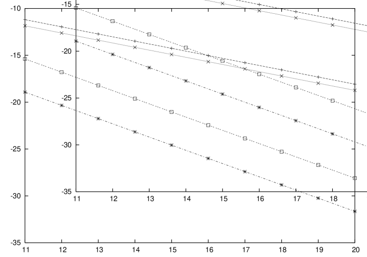
Figure 2: $\log(m^{-1}E)$ vs. $l$ for the ground state, with various values of the bulk and boundary parameters. See Sec. 5.1.3.

In Figure 2 this correction is checked as a function of $\nu=1+1/\lambda$ and of the boundary parameters. On the figure the logarithm of the dimensionless ground state energy is plotted against the dimensionless volume. The upper two lines in descending order are the Lüscher corrections (5.5) for $\nu=1.25,\>b_{+}=-b_{-}=0.1$; and with $a_{+}=1.2\>,\,a_{-}=-0.2$ for the first line, and $a_{+}=1.1\>,\,a_{-}=-0.3$ for the second line. The lower two lines have parameters $\nu=1.5,\>a_{+}=1.2\>,\,a_{-}=-0.2$; and with $b_{+}=-b_{-}=1$ for the first line, while $b_{+}=-b_{-}=0.1$ for the second line. The various boxes are the data of the numerical solution of the NLIE. The agreement is really excellent.

5.2 Excited states

NLIE results for states with 1 and 2 holes, whose UV limits are discussed in Exs. 2 and 3 at the end of Section 4.1, are presented in Figs. 3 and 4, respectively. Note that the values of ${\cal E}$ in the IR limit are 1 and 2, respectively, in agreement with (5.3). Moreover, the values of ${\cal E}$ in the UV limit agree well with (5.2) and with the analytical results for $\Delta_{n}$ given by (2.29), (4.20).

In particular, for the 1-hole states (Fig. 3), we consider integer values $I^{H}=1,2,3,4$; we find that the corresponding hole rapidities $\theta^{H}$ become infinite in the UV limit, and thus, all of these states have $n=0$. The values of ${\cal E}$ in the UV limit are spaced by 1 on account of the additional integer contribution to $\Delta_{n}$ in (4.20): as $I^{H}=I^{H\ \infty}$ increases by 1, so does $\Delta_{n}$. Similarly, for the 2-hole states (Fig. 4), we consider integer values $(I_{1}^{H},I_{2}^{H})=(1,2),(1,3),(1,4),(2,3)$; we find that both hole rapidities become infinite in the UV limit, and thus, the states have $n=-1$. As $I_{1}^{H}+I_{2}^{H}$ increases by 1, so does the limiting UV value of $\Delta_{n}$. Hence, the lowest line is $(I_{1}^{H},I_{2}^{H})=(1,2)$, the second-lowest line is $(1,3)$, and the next two (almost degenerate) are $(2,3)$ and $(1,4)$.

6 Conclusion

Starting from the Bethe Ansatz solution [16, 17, 18] of the XXZ model with general boundary terms, we have derived a nonlinear integral equation for some bulk excited states of the sine-Gordon model on a finite interval with general integrable boundary interactions [10, 11], including boundary terms proportional to $\partial_{y}\varphi$. We have used this NLIE to compute numerically the dimensions of these states as a function of scale, and have checked the UV and IR limits analytically. We have also verified that the ground-state NLIE agrees well with boundary conformal perturbation theory (BCPT), boundary truncated conformal space approach (BTCSA) and the boundary Lüscher formula. An advantage of the latter approaches is that they are not restricted to values of the boundary parameters that obey the constraints (3.4), (4.14). The consistency of the results provides support for the proposed relations between the lattice and continuum boundary parameters.

The result (2.29) for the conformal dimensions of a free massless Boson with Neumann boundary conditions and $\partial_{y}\varphi$ boundary terms, which is “dual” to the corresponding result for a massless Boson with Dirichlet boundary conditions [28, 29], may have applications in other contexts, such as string theory.

There are many issues that remain to be addressed. Among these are the proper treatment of complex (bulk) and imaginary (boundary) sources in the NLIE. While the former problem is in principle understood [4, 8], the latter problem is still not well understood even in the simpler Dirichlet case [8, 36]. Moreover, it would be interesting to extend the comparison of NLIE with BCPT and BTCSA also to excited states.

Appendix A Boundary Conformal Perturbation Theory
and Boundary Truncated Conformal Space Approach

Boundary conformal perturbation theory (BCPT) and boundary truncated conformal space approach (BTCSA) [25, 37] can be applied if the theory is a relevant perturbation of a boundary conformal field theory:

$$L=L_{BCFT}+L_{pert}=L_{BCFT}-\mu_{bulk}\int_{x_{-}}^{x^{+}}\Phi(x,t)dx-\mu_{-}\Psi_{-}(t)-\mu_{+}\Psi_{+}(t)\quad,$$

where $L_{BCFT}$ is the Lagrangian of the UV limiting boundary conformal field theory, $\Phi(x,t)$ is a relevant bulk primary field of weights $(h,\bar{h})$ and $\Psi_{\pm}$ are relevant boundary fields living on the left/right boundaries of the strip with weights $\Delta_{\pm}$. For simplicity we will suppose that $h=\bar{h}=\Delta_{-}=\Delta_{+}=:\Delta.$ and put $x_{-}=0;\;x_{+}=L$.

A.1 Hamiltonian approach

We are interested in the spectrum of the Hamiltonian:

$$H(L)=H_{BCFT}(L)+\mu_{bulk}\int_{0}^{L}\Phi(x,t)dx+\mu_{-}\Psi_{-}(t)+\mu_{+}\Psi_{+}(t)\quad.$$

The volume dependence can be obtained by mapping the system to the upper half plane (UHP) via $z=e^{i\frac{\pi}{L}(x+t)}$, where $t=-iy$ is the Euclidean time. The transformation rules of the primary fields are given by:

$$\Phi(x,t)=\left(\frac{\pi^{2}}{L^{2}}z\bar{z}\right)^{\Delta}\Phi(z,\bar{z})\quad;\quad\Psi_{\pm}(t)=\left(\mp\frac{\pi}{L}z\right)^{\Delta}\Psi(z)\quad,$$ (A.1)

Changing the integration variable to $\theta=\frac{\pi}{L}x$ and taking the Hamiltonian at $t=0$, we have:

$$H(L) = \frac{\pi}{L}\left(L_{0}-\frac{c}{24}\right)+\mu_{bulk}\left(\frac{\pi}{L}\right)^{2\Delta-1}\int_{0}^{\pi}\Phi(e^{i\theta},e^{-i\theta})d\theta$$

$$+ \mu_{-}\left(\frac{\pi}{L}\right)^{\Delta}\Psi_{-}(1)+\mu_{+}\left(\frac{\pi}{L}\right)^{\Delta}\Psi_{+}(-1)\quad,$$

where $L_{0}$ is the spectrum of the boundary conformal field theory with central charge, $c$. The spectrum of $H(L)$ can be calculated at least in two different ways: using perturbative (BCPT) and variational methods (BTCSA).

In the variational method we use, as input, the eigenvectors, $|n\rangle$, of the unperturbed (boundary conformal) Hamiltonian. For practical reasons we consider the eigenvectors having energy less then a given value, $E_{cut}$, and perform the calculation numerically. (Technically this means diagonalizing the truncated Hamiltonian).

Standard perturbation theory gives rise to the following perturbative series for the energy level labeled with its unperturbed UV limiting vector $|n\rangle$,

$$E_{n}(L)=\frac{\pi}{L}\left(E_{|n\rangle}-\frac{c}{24}+\sum_{k=1}^{\infty}c_{k}^{n}(\mu_{bulk},\mu_{\pm},\Delta)\left(\frac{\pi}{L}\right)^{k(\Delta-1)}\right)\quad\,,$$ (A.2)

where $E_{|n\rangle}$ denotes the conformal energy on the UHP. For the ground state the first few terms have the form

$$E_{0}(L)=\frac{\pi}{L}\left(E_{|0\rangle}-\frac{c}{24}+c_{1}^{0}(\mu_{\pm},\Delta)\left(\frac{\pi}{L}\right)^{(\Delta-1)}+c_{2}^{0}(\mu_{bulk},\mu_{\pm},\Delta)\left(\frac{\pi}{L}\right)^{2(\Delta-1)}+\dots\right)\quad,$$ (A.3)

where

$$c_{1}^{0}(\mu_{\pm},\Delta)=\langle 0|\left(\mu_{-}\Psi_{-}(1)+\mu_{+}\Psi_{+}(-1)\right)|0\rangle$$ (A.4)

and

$$c_{2}^{0}(\mu_{bulk},\mu_{\pm},\Delta) = \mu_{bulk}\int_{0}^{\pi}\langle 0|\Phi(e^{i\theta},e^{-i\theta})|0\rangle d\theta$$ (A.5)

$$+\sum_{i,j=\{\pm\}}\mu_{i}\mu_{j}\sum_{n\in\mathcal{H}}\frac{\langle 0|\Psi(i1)|n\rangle\langle n|\Psi(j1)|0\rangle}{E_{|0\rangle}-E_{|n\rangle}}\quad.$$

The large volume behavior of the ground state energy is

$$E_{0}(L)=\epsilon_{bulk}L+\epsilon_{boundary}^{-}+\epsilon_{boundary}^{+}+O(e^{-mL})\quad\textrm{as \quad}L\to\infty\quad.$$

The ground state energy in the NLIE description, however, is normalized differently as $E_{0}^{NLIE}(L)=O(e^{-mL})$ when $L\to\infty$. The correspondence between the two schemes is

$$E_{0}(L)=E_{0}^{NLIE}(L)+\epsilon_{bulk}L+\epsilon_{boundary}^{-}+\epsilon_{boundary}^{+}\quad.$$ (A.6)

A.2 Lagrangian approach

The evaluation of the second order term in the Hamiltonian perturbation theory (A.5) is cumbersome, since we have to sum up the various matrix elements. We can avoid this calculation by doing Lagrangian perturbation theory instead. We compactify the strip in the time-like direction on a circle of radius $R$ and consider the large $R$ limit of the cylinder partition function:

$$Z(L,R)=Tr(e^{-RH(L)})=e^{-RE_{0}(L)}+\dots\quad\textrm{for \quad}R\to\infty\quad.$$

Using the functional integral representation for the partition function with the action, $S=\int L(t)dt=S_{BCFT}+S_{pert}$,

$$Z(L,R) = \int d[\Phi,\Psi_{\pm}]e^{-S}=\int d[\Phi,\Psi_{\pm}]e^{-S_{BCFT}}e^{-S_{pert}}$$

$$= Z_{BCFT}\frac{\int d[\Phi_{\ },\Psi_{\pm}]e^{-S_{BCFT}}e^{-S_{pert}}}{Z_{BCFT}}=Z_{BCFT}\left\langle e^{-S_{pert}}\right\rangle$$

$$= Z_{BCFT}\left\langle\sum_{n=0}^{\infty}\frac{(-S_{pert})^{n}}{n!}\right\rangle\quad.$$

We can obtain the first few perturbative corrections to the ground state energy as

$$-\frac{1}{R}\lim_{R\to\infty}\log(Z(L,R)) = E_{0}(L)=E_{0}^{BCFT}(L)+\sum_{i=\pm}\mu_{i}\langle 0|\Psi_{i}(0)|0\rangle$$

$$+\mu_{bulk}\int_{0}^{L}\langle 0|\Phi(x,0)|0\rangle dx-\frac{1}{2}\sum_{i,j=\{\pm\}}\mu_{i}\mu_{j}\int_{-\infty}^{\infty}\langle 0|\Psi_{i}(0)\Psi_{j}(t)|0\rangle dt+\dots\quad,$$

where the correlators are the connected BCFT correlators. By transforming the various expressions onto the upper half plane we obtain:

$$E_{0}(L) = E_{0}^{BCFT}(L)+\sum_{i}\mu_{i}\left(\frac{\pi}{L}\right)^{\Delta}\langle 0|\Psi_{i}(0)|0\rangle$$

$$+\left(\frac{\pi}{L}\right)^{2\Delta-1}\left[\mu_{bulk}\int_{0}^{\pi}\langle 0|\Phi(e^{i\theta},e^{-i\theta})|0\rangle d\theta-\frac{1}{2}\sum_{i.j}\mu_{i}\mu_{j}\int_{0}^{\infty}duu^{\Delta-1}\langle 0|\Psi_{i}(i1)\Psi_{j}(ju)|0\rangle\right]-\dots$$

where $z=u+iv=re^{i\theta}$. Comparing the result with equations (A.3,A.4,A.5) we can establish the correspondence with the Hamiltonian perturbation theory. Clearly the second order term in (A.5) is summed up. One can compare this term directly by inserting the resolution of the identity $1=\sum_{n}|n\rangle\langle n|$ and using the conformal transformation property of the fields.

In any BCFT, using the $sl_{2}$ invariance of the vacuum, $|0\rangle$, the bulk one point function on the UHP can be put to the form

$$\langle 0|\Phi(e^{i\theta},e^{-i\theta})|0\rangle=\frac{c_{bulk}}{\sin(\theta)^{2\Delta}}\quad,$$ (A.8)

while the boundary two point function can be brought to the form

$$\langle 0|\Psi_{i}(i1)\Psi_{j}((ju)|0\rangle=\frac{c_{ij}}{|1-(i1)\cdot(ju)|^{2\Delta}}\,,$$ (A.9)

where the radial ordering is taken into account. The relevant integrals can be written in terms of the beta function $B(x,y)$, both for the bulk and for $i=j$ and for $i\neq j$ as

$$\int_{0}^{1}du\,u^{x-1}(1-u)^{y-1}=\int_{0}^{\infty}du\,u^{x-1}(1+u)^{-x-y}=B(x,y)=\frac{\Gamma(x)\Gamma(y)}{\Gamma(x+y)}\quad,$$

The first integral converges only for $y>0$ thus $0<\Delta<\frac{1}{2}$ is needed. Collecting all terms, the $c_{2}^{0}$ coefficient is

$$c_{2}^{0}(\mu_{bulk},\mu_{\pm},\Delta) = \mu_{bulk}c_{bulk}\frac{\Gamma(\frac{1}{2}-\Delta)\Gamma(\frac{1}{2})}{\Gamma(1-\Delta)}$$ (A.10)

$$-(\mu_{+}^{2}c_{++}+\mu_{-}^{2}c_{--})\frac{\Gamma(\Delta)\Gamma(1-2\Delta)}{\Gamma(1-\Delta)}-\mu_{-}\mu_{+}c_{+-}\frac{\Gamma^{2}(\Delta)}{\Gamma(2\Delta)}\quad,$$

where only the coefficients $c_{bulk},\,c_{ij}$ are model dependent.

A.3 Boundary sine-Gordon theory

In the sine-Gordon theory the UV limiting BCFT is described by (2.13), the bulk perturbation is given by

$$\Phi(x,t)=\frac{1}{2}(V_{\beta}(x,t)+V_{-\beta}(x,t))\quad;\quad V_{\beta}(z,\bar{z})=n(z,\bar{z}):e^{i\beta\varphi(z,\bar{z})}:\quad,$$

while the boundary by

$$\Psi_{\pm}(t)=\frac{1}{2}\left(e^{-i\frac{\beta\varphi_{0}^{\pm}}{2}}U_{\frac{\beta}{2}}(t)+e^{i\frac{\beta\varphi_{0}^{\pm}}{2}}U_{-\frac{\beta}{2}}(t)\right)\quad;\quad U_{\frac{\beta}{2}}(u)=:e^{i\frac{\beta}{2}\varphi(u,u)}:\quad,$$

and $\Delta=\frac{\beta^{2}}{8\pi}$, see [37] for the details. Since the bulk, $V_{\beta}(z,\bar{z})$, and boundary, $U_{\frac{\beta}{2}}(u)$, vertex operators change the eigenvalue of $\pi_{0}$ by $\beta$ and $\frac{\beta}{2}$, respectively, only even $c$ coefficients are nonzero in the expansion (A.2). Moreover, the vacuum expectation value of $\Phi$ is also zero (A.8), thus the leading perturbative contribution comes from the boundary two point function part of (A.2). In the boundary sine-Gordon theory with nonzero $\kappa:=\kappa_{+}-\kappa_{-}$ the vacuum is not $sl_{2}$-invariant and thus (A.9) has to be modified. In general for a theory with a non $sl_{2}$-invariant vacuum one has to compute the four point functions, instead of the two point function, and extract the relevant matrix element from them. Alternatively, in our case, one can also use the mode expansion of the field (2.16) together with the commutation relations (2.18) to obtain:

$$\langle 0|U_{\pm\frac{\beta}{2}}(i1)U_{\mp\frac{\beta}{2}}((ju)|0\rangle=\frac{|u|^{\mp\frac{4\kappa\Delta}{\beta}}}{|1-(i1)\cdot(ju)|^{2\Delta}}\quad.$$

This modifies (A.10) and gives the leading corrections:

$$c_{2}^{0}(\mu_{\pm},\Delta,\kappa) = -\frac{1}{2}\left[(\mu_{+}^{2}+\mu_{-}^{2})\frac{\Gamma(1-2\Delta)}{2}\left(\frac{\Gamma(\Delta+\frac{4\kappa\Delta}{\beta})}{\Gamma(1+\frac{4\kappa\Delta}{\beta}-\Delta)}+\frac{\Gamma(\Delta-\frac{4\kappa\Delta}{\beta})}{\Gamma(1-\frac{4\kappa\Delta}{\beta}-\Delta)}\right)\right.$$ (A.11)

$$\left.+\mu_{-}\mu_{+}\cos\frac{\beta}{2}(\varphi_{0}^{+}-\varphi_{0}^{-})\frac{\Gamma(\Delta+\frac{4\kappa\Delta}{\beta})\Gamma(\Delta-\frac{4\kappa\Delta}{\beta})}{\Gamma(2\Delta)}\right]\quad.$$

Although the derivation of this formula assumes that $0<\Delta<1/2$, the final result is analytic in $\Delta$ (with possible poles). Therefore it has an analytic continuation for $\Delta>1/2$, which, since the NLIE is also analytic in $\Delta$, must coincide with the NLIE result. This is confirmed by experience with the NLIE for bulk sine-Gordon and bulk supersymmetric sine-Gordon models. Using the UV-IR relation (2.46), (2.47) and the mass-gap formula (cf. [38])

$$\mu_{bulk}=m^{2-2\Delta}\frac{2\Gamma(\Delta)}{\pi\Gamma(1-\Delta)}\left(\frac{\sqrt{\pi}\Gamma\left(\frac{1}{2(1-\Delta)}\right)}{2\Gamma\left(\frac{\Delta}{2(1-\Delta)}\right)}\right)^{2-2\Delta}\quad,$$ (A.12)

where $m$ is the soliton mass, $c_{2}^{0}(\mu_{\pm},\Delta,\kappa)$ can be rewritten in terms of the IR parameters.

Figure 1: $-c_{eff}/24$ vs. $\log l$ for ground state (0 holes), with parameter values $\nu=1.93$, $a_{+}=1.8$, $a_{-}=-0.9$, and $b_{+}=-b_{-}=0.41444$. See Ex. 1 in Sec. 4.1, and Sec. 5.1.

Figure 3: ${\cal E}$ vs. $\log l$ for 1-hole states with integer values $I^{H}=1,2,3,4$, and with parameter values $\nu=1.93$, $a_{+}=1.8$, $a_{-}=1.9$, and $b_{+}=-b_{-}=0.41444$. See Ex. 2 in Sec. 4.1, and Sec. 5.2.

Figure 4: ${\cal E}$ vs. $\log l$ for 2-hole states with integer values $(I_{1}^{H},I_{2}^{H})=(1,2),(1,3),(1,4),(2,3)$, and with parameter values $\nu=2.13$, $a_{+}=1.8$, $a_{-}=-0.9$, and $b_{+}=-b_{-}=0.50357$. See Ex. 3 in Sec. 4.1, and Sec. 5.2.

References

- [1] A. Klümper, M.T. Batchelor and P.A. Pearce, J. Phys. A24 (1991) 3111.
- [2] C. Destri and H.J. de Vega, Phys. Rev. Lett. 69 (1992) 2313.
- [3] D. Fioravanti, A. Mariottini, E. Quattrini and F. Ravanini, Phys. Lett. B390 (1997) 243.
- [4] C. Destri and H.J. de Vega, Nucl. Phys. B504 (1997) 621.
- [5] G. Feverati, F. Ravanini and G. Takacs, Nucl. Phys. B540 (1999) 543.
- [6] G. Feverati, “Finite volume spectrum of sine-Gordon model and its restrictions,” hep-th/0001172.
- [7] A. LeClair, G. Mussardo, H. Saleur and S. Skorik, Nucl. Phys. B453 (1995) 581.
- [8] C. Ahn, M. Bellacosa and F. Ravanini, Phys. Lett. B595 (2004) 537.
- [9] C. Ahn and R.I. Nepomechie, Nucl. Phys. B676 (2004) 637.
- [10] E.K. Sklyanin, Funct. Anal. Appl. 21 (1987) 164.
- [11] S. Ghoshal and A.B. Zamolodchikov, Int. J. Mod. Phys. A9 (1994) 3841.
- [12] Z. Bajnok, L. Palla and G. Takács, Nucl. Phys. B622 (2002) 565.
- [13] J.-S. Caux, H. Saleur and F. Siano, Phys. Rev. Lett. 88 (2002) 106402.
- [14] J.-S. Caux, H. Saleur and F. Siano, Nucl. Phys. B672 (2003) 411.
- [15] T. Lee and C. Rim, Nucl. Phys. B672 (2003) 487.
- [16] R.I. Nepomechie, J. Stat. Phys. 111 (2003) 1363; J. Phys. A37 (2004) 433.
- [17] J. Cao, H.-Q. Lin, K.-J. Shi and Y. Wang, “Exact solutions and elementary excitations in the XXZ spin chain with unparallel boundary fields,” cond-mat/0212163; Nucl. Phys. 663 (2003) 487.
- [18] R.I. Nepomechie and F. Ravanini, J. Phys. A36 (2003) 11391; Addendum, J. Phys. A37 (2004) 1945.
- [19] H.J. de Vega and A. González-Ruiz, J. Phys. A26 (1993) L519.
- [20] M. Gaudin, Phys. Rev. A4 (1971) 386; La fonction d’onde de Bethe (Masson, 1983).
- [21] F.C. Alcaraz, M.N. Barber, M.T. Batchelor, R.J. Baxter and G.R.W. Quispel, J. Phys. A20 (1987) 6397.
- [22] E.K. Sklyanin, J. Phys. A21 (1988) 2375.
- [23] Al.B. Zamolodchikov, invited talk at the 4th Bologna Workshop, June 1999.
- [24] V.P. Yurov and Al.B. Zamolodchikov, Int. J. Mod. Phys. A5 (1990) 3221.
- [25] P. Dorey, A. Pocklington, R.Tateo, G. Watts, Nucl. Phys. B525 (1998) 641.
- [26] M. Lüscher, Comm. Math. Phys. 104 (1986) 177; ibid, 105 (1986) 153.
- [27] Z. Bajnok, L. Palla and G. Takács, “Finite size effects in quantum field theories with boundary from scattering data,” hep-th/0412192.
- [28] H. Saleur, “Lectures on nonperturbative field theory and quantum impurity problems,” cond-mat/9812110.
- [29] I. Affleck, M. Oshikawa and H. Saleur, Nucl. Phys. B594 (2001) 535.
- [30] C. Destri and H.J. de Vega, Nucl. Phys. B290 (1987) 363.
- [31] H.J. de Vega, Int. J. Mod. Phys. A4 (1989) 2371.
- [32] N.Yu. Reshetikhin and H. Saleur, Nucl. Phys. B419 (1994) 507.
- [33] A. Doikou, L. Mezincescu and R.I. Nepomechie, J. Phys. A30 (1997) L507.
- [34] P. Fendley and H. Saleur, Nucl. Phys. B428 (1994) 681.
- [35] P.A. Pearce, L. Chim and C. Ahn, Nucl. Phys. B601 (2001) 539.
- [36] S. Skorik and H. Saleur, J. Phys. A28 (1995) 6605.
- [37] Z. Bajnok, L. Palla and G. Takács, Nucl. Phys. B614 (2001) 405.
- [38] Al.B. Zamolodchikov, Int. J. Mod. Phys. A10 (1995) 1125.