A Variational Perturbation Approach
to One-Point Functions in QFT

Abstract

In this paper, we develop a variational perturbation (VP) scheme for calculating vacuum expectation values (VEVs) of local fields in quantum field theories. For a comparatively general scalar field model, the VEV of a comparatively general local field is expanded and truncated at second order in the VP scheme. The resultant truncated expressions (we call Gaussian smearing formulae) consist mainly of Gaussian transforms of the local-field function, the model-potential function and their derivatives, and so can be used to skip calculations on path integrals in a concrete theory. As an application, the VP expansion series of the VEV of a local exponential field in the sine- and sinh-Gordon field theories is truncated and derived up to second order equivalently by directly performing the VP scheme, by finishing ordinary integrations in the Gaussian smearing formulae, and by borrowing Feynman diagrammatic technique, respectively. Furthermore, the one-order VP results of the VEV in the two-dimensional sine- and sinh-Gordon field theories are numerically calculated and compared with the exact results conjectured by Lukyanov, Zamolodchikov $et\;al.$, or with the one-order perturbative results obtained by Poghossian. The comparisons provide a strong support to the conjectured exact formulae and illustrate non-perturbability of the VP scheme.

I Introduction

Green’s functions and correlation functions in quantum field theory(QFT), statistical mechanics and condensed matter physics are closely related to experimental studies on macroscopic matter systems and elementary particles 1 . Because of the existence of an operator-product-expansion algebra, various multi-point Green’s or correlation functions with the points approaching each other can be reduced down to one-point functions or vacuum expectation values (VEVs) of local fields 2 . On the other hand, as far as VEVs themselves go, they determine the linear responses of statistical-mechanics systems to external fields, and contain non-perturbative information about QFT, which is not accessible through a direct investigation in the conformal perturbation theory. Hence the problem of calculating the VEVs of local fields is of fundamental significance.

There exist some methods for calculating the VEVs of local fields. For an integrable QFT which can be considered as a conformal field theory perturbed by some operator, the VEV of the perturbing operator can be exactly obtained with the help of the thermodynamic Bethe Ansatz approach 3 ; 4 . This kind of exact calculation succeeded only in very few cases 4 . Nevertheless, S. Lukyanov and A. Zamolodchikov made a significant progress in 1997 and conjectured the exact VEV of an exponential field in the two-dimensional sine-Gordon (sG) and sinh-Gordon (shG) field theories 4 . This progress has led to the use of reflection relation 5 and accordingly exact VEVs of local fields in many perturbed conformal field theories without and with boundaries have been proposed 6 ; 7 through solving the reflection relations. Furthermore, these conjectured exact VEVs have again been employed to give VEVs of local fields in some other QFTs by making use of quantum group restriction existed between the relevant QFTs 6 ; 8 . Besides, recently, because of the peculiarity in super-Liouville theories with boundary, conformal bootstrap method 9 and Modular transformation method 10 were used to derive one-point functions of bulk and boundary operators. For the boundary scaling Lee-Yang model, one-point functions of bulk and boundary fields were approximated by using the truncated conformal space approach and the form-factor expansion 11 . Additionally, in order to check those exact predictions, perturbation theory 12 and some numerical methods based on the truncated conformal space approach 13 were adopted to calculate the VEVs.

Obviously, since VEVs of local fields in QFT are non-perturbative objects, general and systematical non-perturbation methods of directly calculating VEVs are needed and such tools are also necessary for independently checking those predictions on the exact VEVs. We feel that a variational perturbation (VP) theory 14 can afford such a tool. The VP theory can be regarded as some mixture of conventional perturbation theory and variational method. As is well known, the perturbation theory is a systematical approximation tool and results from it can be improved order by order. Meanwhile, the variational method is feasible and effective as well as valid for any coupling (the weak or the strong). These two methods have been dominating approximation calculations in theoretical researches for a long time, being two standard approximation tools. However, the perturbation theory is valid only for very weak coupling at most and the variational method gives no indication of the error in its resultant value. In order to collect their merits, avoid their drawbacks, and, of course, to develop a systematical non-perturbative tool, a primitive idea of the VP theory for simply combining the conventional perturbation theory with the variational method was proposed as a tool of solving stationary Schrödinger equation in 1955 15 (which can even date back to even twenty more years earlier 16 ). This naive combination has been applied to many fields in physics (see references in Ref. 14 ; 17 ; 18 ). It amounts to an expansion around variational approximate result and the variational parameter in the expansion is determined with the one-order result by variational method. This primitive VP theory really produces non-perturbative results which are valid for any coupling strength and can be improved order by order. Nevertheless, the naive combination of the perturbative and variational methods does not provide a convergent tool because the variational parameter is independent of the approximate order 14 . In 1981 or so, the principle of minimal sensitivity (PMS) 19 was proposed by P. M. Steveson (Possibly, earlier in the middle 1970s, a similar principle was proposed in Mosc. Univ. Phys. Bull. 31, 10(1976) by V. I. Yukalov) and can be used to determine an auxiliary parameter (the aforementioned variational parameter) which is artificially introduced into the VP theory. The VP theory with the PMS determines the parameter order by order (see next section) and is believed to be a fast convergent theory 14 . Now, as a systematical and non-perturbative tool, it has developed with many equivalent practical schemes to calculate energies, free energies and effective potentials of systems, and has been applied to QFT, condensed matter physics, statistical mechanics, chemical physics, and so on 14 ; 17 ; 18 (for a full list, to see references in Refs. 14 ; 17 ; 18 ). In this paper, we intend to develop a VP scheme to calculate the VEVs of local fields in QFT.

In sect.II, we will develop the VP scheme in a general way. For universality and definiteness, we shall consider a class of systems, scalar field systems or Fermi field systems which can be bosonized, with the Lagrangian density 20

$${\cal L}_{x}={\frac{1}{2}}\partial_{\mu}\phi_{x}\partial^{\mu}\phi_{x}-V(\phi_{x})\;.$$ (1)

In Eq.(1), the subscript $x=(\vec{x},t)$ represents the coordinates in a $(D+1)$-dimensional Minkowski space, $\partial_{\mu}$ and $\partial^{\mu}$ are the corresponding covariant derivatives, and $\phi_{x}\equiv\phi(x)$ the scalar field at $x$. The potential $V(\phi_{x})$ in Eq.(1) is assumed to have a Fourier representation in a sense of tempered distributions 21 ,

$$V(\phi_{x})=\int{\frac{d\omega}{\sqrt{2\pi}}}\tilde{V}(\omega)e^{i\omega\phi_{x}}\;.$$ (2)

Speaking roughly, this requires that the integral $\int^{\infty}_{-\infty}V(\alpha)e^{-C\alpha^{2}}d\alpha$ with a positive constant $C$ is finite. This shouldn’t be regarded as a limitation, and, as a matter of fact, quite a number of model potentials possess the property, such as the potentials of polynomial models, sG and shG models, Bullough-Dodd model, Liouville model, two models discussed in Ref. 22 , and so on. By the way, a similar general model was studied in Ref. 2 . For comparisons with existed work, we will work in a $\nu$-dimensional Euclidean space with $\nu\equiv(D+1)$. Through the time continuation $t\to-i\tau$ with $\tau$ the Euclidean time, a point $x$ in the Minkowski space is transformed into a point $\vec{r}=(\vec{x},\tau)$ in the Euclidean space. For universality and definiteness again, we will also assume that the local field has a Fourier representation,

$${\cal O}(\phi_{\vec{r}_{0}})=\int{\frac{d\Omega}{\sqrt{2\pi}}}{\tilde{\cal O}}(\Omega)e^{i\Omega\phi_{\vec{r}_{0}}}\;,$$ (3)

at least in a sense of tempered distributions. Here, $\vec{r}_{0}=(\vec{x}_{0},\tau_{0})$ is a given point in the Euclidean space. It is evident that such a local field is a comparatively general one. In the present paper, based on the VP scheme in Ref. 18 (the scheme stemmed from the Okopinska’s optimized expansion 23 , and was proposed by Stancu and Stevenson 24 ), we will develop a VP scheme to calculate the VEV of the local field ${\cal O}(\phi_{\vec{r}_{0}})$, Eq.(3), for the field theory Eq.(1) in the $\nu$-dimensional Euclidean space. In subsection $A$ of next section, we will state the VP scheme. It embraces mainly two key steps: one is the VP expansion on the VEVs with an auxiliary parameter introduced, and another is the determination of the auxiliary parameter in the expressions truncated from the VP expansion series. It is the truncated expressions that give rise to the VP approximate results of VEVs up to the truncated order. Then, in subsection $B$ of next section, the truncated expansions of the VEV of ${\cal O}(\phi_{\vec{r}_{0}})$ in the field theory, Eq.(1), will concretely be derived up to the second order. One will see that the resultant truncated expressions up to the second order are composed mainly of Gaussian transforms of the local field ${\cal O}(\phi)$ and the potential $V(\phi)$ as well as their derivatives, and we will call them Gaussian smearing formulae. For, at least, any scalar field theory which is involved in the model with Eq.(1), one can give VP approximated VEVs of ${\cal O}(\phi_{\vec{r}_{0}})$ up to the second order just by finishing ordinary integrations appeared in the Gaussian smearing formulae instead of calculating path integrals in the definitions of the VEVs. This point is the main reason why we are interested in the general model, Eq.(1) and the general local fields, Eq.(3). We should point out that since the QFT with Eq.(1) is not a concrete theory, so we will not carry out the other key step to determine the adjustable parameter in the Gaussian smearing formulae. Section IV will provide such an example on how to determine the auxiliary parameter by the PMS.

About the VP scheme, the renormalization problem need to be explained here. Since a bare field theory is full of divergences and makes no senses, we have to face those divergences appeared in the Gaussian smearing formulae and perform a necessary renormalization procedure to make the formulae finite before performing the second key step with the PMS in the VP scheme. Generally, the renormalization procedure is usually very complicated, and is similar to those in perturbative theory 24 . In order to concentrate our attention at developing the VP theory, we do not hope to be plagued with the complicated renormalization problems of QFT, but we certainly hope to give a finite example for the Gaussian smearing formulae. Fortunately, for any two-dimensional scalar field theory with non-derivative interactions, all ultraviolet divergences can be removed by normal-ordering the Hamiltonian 25 ; 2 . This fact led to a simple renormalization scheme for two-dimensional field theory, the Coleman’s normal-ordering renormalization prescription. Furthermore, this convenient renormalization prescription has been generalized to path integrals of Minkowski and Euclidean formalisms in Ref. 25a and Ref. 20 (2002), respectively. Hence, this prescription was used in Ref. 18 and will be adopted in the present paper. One will see that the Gaussian smearing formulae are full of no explicit divergences for the case of $\nu=2$ and so, generally, no further renormalization procedures are needed for this case.

As an application of the scheme, Sections III and IV will calculate the VEV of the local exponential field $e^{ia\phi_{\vec{r}_{0}}}$ in the sG field theory, $G_{a}$, with $a$ a parameter. The sG model, which appeared early in 1909 26 , is closely related to lots of problems in mathematics and physics, and has been extensively studied. For the general local field ${\cal O}(\phi_{\vec{r}_{0}})$, Eq.(3), its VEV can closely be related to that of an local exponential field, and so the problem of calculating the VEVs of the local exponential field is important. In 1997, through direct calculations in the sG field theory at the coupling $\beta^{2}\to 0$ ( semi-classical limit) and in the free-fermion theory (equivalent version of the sG field theory at $\beta^{2}={\frac{1}{2}}$), and through the exact specific free energy for the sG field theory, Lukyanov and Zamolodchikov obtained the exact $G_{a}$ for the following three special cases: $\beta\to 0$ (semi-classical limit), $\beta={\frac{1}{2}}$ and $a=\beta$, respectively 4 . And then, in the same paper, starting from those exact expressions for the special cases, they guessed an exact formula for $G_{a}$ in the two-dimensional sG field theory at any $\beta^{2}<1$ and $|Re(a)|<1/(2\beta)$. Obviously, it is worthwhile checking the conjectured exact formula. In order to do so, in the same paper, defining “fully connected” one-point functions, $\sigma_{2n}$, from the VEVs of even-power fields $\phi^{2n}$, they showed that $\sigma_{2}$ and $\sigma_{4}$ from the above-mentioned exact formula agree with those from perturbation theory for the sG field theory up to $\beta^{4}$ and that $\sigma_{2}$ agrees with the corresponding one-point function from perturbation theory up to $g$ the coupling in the massive Thirring model, which is the fermion version of the sG field theory 25 (1975). Furthermore, it was found that the conjectured exact formula can be reobtained from the reflection relations 5 , supporting it indirectly. Slightly later, in 2000, checks from perturbation theories in both an angular and a radial quantization approaches for the massive Thirring model indicated that the perturbation result up to $g$ exactly coincides with the corresponding result obtained by expanding the exact formula according to the coupling $g$ 12 (2000). In the same year, a numerical study for the model at a finite volume also provides evidence for the conjectured exact formula 13 (2000). In brief, up to now, the conjectured exact formula for $G_{a}$ in the two-dimensional sG field theory has been completely checked for the case of $\beta^{2}\to{\frac{1}{2}}$ ($g\to 0$ is equivalent to $\beta^{2}\to{\frac{1}{2}}$, See Eq.(67)), and received some indirect evidences for its validity. So, besides providing an example of applying the VP scheme, investigations on $G_{a}$ will also give the conjectured formula a direct check for the cases of $\beta^{2}\not={\frac{1}{2}}$ (Ref. 4 has provided a partial check for $\beta\to 0$).

In section III, we will derive the expressions truncated from the VP expansion series on $G_{a}$ at the second order. It will be done in three ways. Subsection $A$ will directly perform the VP expansion on $G_{a}$ and then truncate the expansion series at the second order. Since the sG and shG field theories are involved in the class of QFTs, Eq.(1), so, in subsection $B$, the truncated expressions of $G_{a}$ up to second order will be recalculated by finishing those ordinary integrations existed in the Gaussian smearing formulae in Section II. The results are identical to those obtained in subsection $A$. Thus, these calculations check and confirm the correctness, usefulness and simplicity of the Gaussian smearing formulae in Section II. Besides, the VP expansion procedure is formally similar to conventional perturbative expansion, and so the Feynman diagrammatic techniques for perturbative theory, which have developed very well up to now, can be borrowed into the VP expansion. Subsection $C$ will provide such a calculation on $G_{a}$ up to the second order in the VP expansion, and the resultant expressions are same as in Subsection $A$ and $B$.

The resultant expressions in Sections II and III are not the final VP approximate results because the other crucial step of the VP scheme is not yet performed to determine the auxiliary parameter by the PMS. As was aforementioned, Sect. IV will do it by considering the truncated expressions up to the first order in Sect. III and treat only the case of $\nu=2$. The sG field theory can be transformed into the shG field theory, and so the one-order VP results on the VEVs of the exponential fields in the two-dimensional both sG and shG field theories will numerically calculated and be completely compared with the conjectured exact results. For the sG model, we will also compare the one-order VP results here with those from a perturbation theory in Ref. 12 (Poghossian). These comparisons, albeit just the one-order results are considered, not only give a strong support for the conjectured exact results but also indicate usefulness and non-perturbability of the VP scheme here for calculating one-point functions. By the way, the VP approximate result up to the second order on the VEV of the exponential fields in the two-dimensional sG field theories has briefly been reported in Ref. 27 , and has a less error to the conjectured exact results than the one-order result. This gives a sign for the convergency of the VP scheme here.

Briefly, next section, we will develop the VP scheme by calculating the VEV’s of the local field, Eq.(3), in the QFT, Eq.(1), and Sect. III and IV will provide an application of the scheme to the sG and shG field theories. A brief conclusion will be made in Sect. V.

II The VP Approach to VEVs of Local Fields in QFT

As was stated in the introduction, we will first state the VP scheme in subsection $A$, and then derive the first three terms in the VP expansion series in subsection $B$.

II.1 the VP Scheme

The generating functional is usually the start of discussing a QFT and will be the basis for the purpose in the present paper. In this subsection, we will first introduce it, then state our VP scheme.

For any field theory, one can use either the Minkowskian formalism or Euclidean formalism to study it 28 . Here, we choose to have our discussion in Euclidean formalism. The Euclidean Lagrangian corresponding to the Minkowskian Lagrangian, Eq.(1), is

$${\cal L}_{\vec{r}}={\frac{1}{2}}\nabla_{\vec{r}}\phi_{\vec{r}}\nabla_{\vec{r}}\phi_{\vec{r}}+V(\phi_{\vec{r}})\;,$$ (4)

which has the same form with the Hamiltonian density of Eq.(1) in $\nu+1$ spacetime. In Euclidean formalism, the corresponding generating functional takes the following form 2 :

$$Z[J]=\int{\cal D}\phi\exp\{-\int d^{\nu}\vec{r}\ [{\frac{1}{2}}\nabla_{\vec{r}}\phi_{\vec{r}}\nabla_{\vec{r}}\phi_{\vec{r}}+V(\phi_{\vec{r}})-J_{\vec{r}}\phi_{\vec{r}}\;]\}\;,$$ (5)

where, $\nabla_{\vec{r}}$ is the gradient in the $\nu$-dimensional Euclidean space, $J_{\vec{r}}$ an external source at $\vec{r}$, and ${\cal D}\phi$ the functional measure. Generally, for an interacting system, the right side hand of Eq.(5) can not exactly be calculated. But for a free field system with $V(\phi_{\vec{r}})={\frac{1}{2}}\mu^{2}\phi_{\vec{r}}^{2}$, its generating functional is exactly calculable and plays a crucial role in the VP theory and relevant calculations. For the convenience of later uses, we write down its result as follows 2

$$Z_{\mu}[J] = \int{\cal D}\phi\exp\{-\int d^{\nu}\vec{r}\ [\ {\frac{1}{2}}\nabla_{\vec{r}}\phi_{\vec{r}}\nabla_{\vec{r}}\phi_{\vec{r}}+{\frac{1}{2}}\mu^{2}\phi_{\vec{r}}^{2}-J_{\vec{r}}\phi_{\vec{r}}\ ]\}$$ (6)

$$= \exp\{-{\frac{1}{2}}\int d^{\nu}\vec{r}\;I_{(0)}(\mu^{2})\}\exp\{{\frac{1}{2}}Jf^{-1}J\}\;.$$

Here,

$$I_{(n)}(Q^{2})\equiv\Biggl{\{}\begin{array}[]{ll}\int{\frac{d^{\nu}\vec{p}}{(2\pi)^{2}}}{\frac{1}{(p^{2}+Q^{2})^{n}}}\;,&\ \ \ \ \ {\rm for}\ \ n\not=0\\ \int{\frac{d^{\nu}\vec{p}}{(2\pi)^{2}}}\ln(p^{2}+Q^{2})\;,&\ \ \ \ \ {\rm for}\ \ n=0\end{array}$$

with $\vec{p}$ momentum and $p=|\vec{p}|$ and $Jf^{-1}J\equiv\int d^{\nu}\vec{r}^{\prime}d^{\nu}\vec{r}^{\prime\prime}J_{\vec{r}^{\prime}}f^{-1}_{\vec{r}^{\prime}\vec{r}^{\prime\prime}}J_{\vec{r}^{\prime\prime}}$ with 24 (1990)

$$f^{-1}_{\vec{r}^{\prime}\vec{r}^{\prime\prime}}\equiv\int{\frac{d^{\nu}\vec{p}}{(2\pi)^{\nu}}}{\frac{1}{p^{2}+\mu^{2}}}\;e^{i\vec{p}\cdot(\vec{r}^{\prime\prime}-\vec{r}^{\prime})}={\frac{\mu^{\nu/2-1}}{(2\pi)^{\nu/2}|\vec{r}^{\prime\prime}-\vec{r}^{\prime}|^{\nu/2-1}}}K_{\nu/2-1}(\mu|\vec{r}^{\prime\prime}-\vec{r}^{\prime}|)\;.$$ (8)

In Eq.(7), $K_{n}(z)$ is the $n$th-order modified Bessel function of the second kind.

Now we address ourselves to the VEVs. For a local field ${\cal O}(\phi_{\vec{r}_{0}})$, its VEV in the theory with Eq.(4) is defined as follows 4

$${\bar{\cal O}}\equiv<{\cal O}(\phi_{\vec{r}_{0}})>\equiv{\frac{\int{\cal D}\phi{\cal O}(\phi_{\vec{r}_{0}})\exp\{-\int d^{\nu}\vec{r}{\cal L}_{\vec{r}}\}}{\int{\cal D}\phi\exp\{-\int d^{2}\vec{r}{\cal L}_{\vec{r}}\}}}\;.$$ (9)

In general, ${\bar{\cal O}}$ in last equation cannot be exactly calculated and one has to manage to design some approximate tool to attack it.

According to Eqs.(3),(4) and (5), ${\bar{\cal O}}$ in Eq.(8) can easily be rewritten as

$${\bar{\cal O}}=\int{\frac{d\Omega}{\sqrt{2\pi}}}{\tilde{\cal O}}(\Omega){\frac{Z[J]_{J_{\vec{r}}=i\Omega\delta(\vec{r}-\vec{r}_{0})}}{Z[J=0]}}\;.$$ (10)

In the numerator of the integrand in Eq.(9), the subscript means that $i\Omega\delta(\vec{r}-\vec{r}_{0})$ takes the place of $J_{\vec{r}}$ in $Z[J]$. Hence, ${\bar{\cal O}}$ can be obtained via calculating the generating functional. Luckily, the calculation of effective potential has stimulated the establishment of several VP expansion schemes on the generating functional (see Refs. 14 ; 17 and references therein), and they can possibly be developed to calculate ${\bar{\cal O}}$. Next, we will generalize the VP scheme in the Ref. 18 (a very slightly different version of that in Ref. 24 ) to calculate ${\bar{\cal O}}$.

As was stated in the introduction, the Coleman’s normal-ordering renormalization prescription will be adopted. That is, the Euclidean Lagrangian in the exponential in Eq.(5) will be replaced by the following normal-ordered form with respect to an arbitrary normal-ordering mass $\cal M$ 20 (2002),

$$-{\frac{1}{2}}I_{(0)}({\cal M}^{2})+{\frac{1}{2}}{\cal M}^{2}I_{(1)}({\cal M}^{2})+{\frac{1}{2}}\nabla_{\vec{r}}\phi_{\vec{r}}\nabla_{\vec{r}}\phi_{\vec{r}}-J_{\vec{r}}\phi_{\vec{r}}+\int{\frac{d\omega}{\sqrt{2\pi}}}\tilde{V}(\omega)e^{i\omega\phi_{\vec{r}}}e^{{\frac{1}{2}}\omega^{2}I_{(1)}({\cal M}^{2})}\;.$$

In the above expression, the last term is the normal-ordered form of $V(\phi_{\vec{r}})$, and can be got by using Eq.(2) and the Baker-Hausdorff formula $e^{A+B}=e^{A}e^{B}e^{-[A,B]}$ with the commutator $[A,B]$ some c-number. So, $Z[J]$ is turned into the following form :

$$Z[J] = \exp\{\int d^{\nu}r[{\frac{1}{2}}I_{(0)}({\cal M}^{2})-{\frac{1}{2}}{\cal M}^{2}I_{(1)}({\cal M}^{2})]\}\int{\cal D}\phi$$ (11)

$$\times\exp\{-\int d^{\nu}\vec{r}\ [{\frac{1}{2}}\nabla_{\vec{r}}\phi_{\vec{r}}\nabla_{\vec{r}}\phi_{\vec{r}}-J_{\vec{r}}\phi_{\vec{r}}+\int{\frac{d\omega}{\sqrt{2\pi}}}\tilde{V}(\omega)e^{i\omega\phi_{\vec{r}}}e^{{\frac{1}{2}}\omega^{2}I_{(1)}({\cal M}^{2})}]\}\;.$$

Eq.(10) is nothing but Eq.(11) of Ref. 20 (2002) in notations here. Thus, for the case of two dimensions, the fields and the model parameters, such as mass and couplings, are now finite 25 ; 2 (for simplicity, we use the same symbols as those in the bare Lagrangian, Eq.(4)).

Now we further modify $Z[J]$ in Eq.(10) by following Ref. 18 or 20 (2002)(only without shifting the field, for simplicity). First, a parameter $\mu$ is introduced by adding a vanishing term$\int d^{\nu}\vec{r}{\frac{1}{2}}\phi_{\vec{r}}(\mu^{2}-\mu^{2})\phi_{\vec{r}}$ into the exponent of the functional integral in Eq.(10). This way of introducing the artificial $\mu$ was used several decades ago 28b . Then, rearrange the exponent into a free-field part (with a mass being the introduced parameter $\mu$) plus a new interacting part. Finally insert a formal expansion factor $\epsilon$ in front of the interacting part. Consequently, $Z[J]$ is turned into the following form

$$Z[J;\epsilon] = \exp\{\int d^{\nu}\vec{r}\;[{\frac{1}{2}}I_{(0)}[M^{2}]-{\frac{1}{2}}M^{2}I_{(1)}[M^{2}]]\}$$ (12)

$$\times\int{\cal D}\phi\exp\{-\int d^{\nu}\vec{r}[{\frac{1}{2}}\phi_{\vec{r}}(-\nabla^{2}_{\vec{r}}+\mu^{2})\phi_{\vec{r}}+\epsilon{\cal H}_{I}(\phi_{\vec{r}},\mu)-J_{r}\phi_{\vec{r}}]\}$$

$$= \exp\{\int d^{\nu}\vec{r}\;[{\frac{1}{2}}I_{(0)}[M^{2}]-{\frac{1}{2}}M^{2}I_{(1)}[M^{2}]]\}$$

$$\times\int{\cal D}\phi\exp\{-\epsilon\int d^{\nu}\vec{r}\;{\cal H}_{I}({\frac{\delta}{\delta J_{\vec{r}}}},\mu)\}\exp\{-\int d^{\nu}\vec{r}[{\frac{1}{2}}\phi_{\vec{r}}(-\nabla^{2}_{\vec{r}}+\mu^{2})\phi_{\vec{r}}-J_{r}\phi_{\vec{r}}]\}$$

$$= \exp\{-\int d^{\nu}\vec{r}\;[{\frac{1}{2}}I_{(0)}(\mu^{2})-{\frac{1}{2}}I_{(0)}({\cal M}^{2})+{\frac{1}{2}}{\cal M}^{2}I_{(1)}({\cal M}^{2})]\}$$

$$\times\exp\{-\epsilon\int d^{\nu}\vec{r}\;{\cal H}_{I}({\frac{\delta}{\delta J_{\vec{r}}}},\mu)\}\exp\{{\frac{1}{2}}Jf^{-1}J\}\;$$

with the new interacting part

$${\cal H}_{I}(\phi_{\vec{r}},\mu)=-{\frac{1}{2}}\mu^{2}\phi_{\vec{r}}^{2}+\int{\frac{d\omega}{\sqrt{2\pi}}}\tilde{V}(\omega)e^{i\omega\phi_{\vec{r}}}e^{{\frac{1}{2}}\omega^{2}I_{(1)}({\cal M}^{2})}\;.$$ (13)

In writing down Eq.(11), we have employed the result Eq.(6). Note that extrapolating $Z[J;\epsilon]$ to $\epsilon=1$, one recovers $Z[J]$ in Eq.(10).

Expanding $\exp\{-\epsilon\int d^{\nu}\vec{r}\;{\cal H}_{I}({\frac{\delta}{\delta J_{\vec{r}}}},\mu)\}$ in Eq.(11) into a series in $\epsilon$, one has

$$Z[J;\epsilon] = \exp\{-\int d^{\nu}\vec{r}\;[{\frac{1}{2}}I_{(0)}(\mu^{2})-{\frac{1}{2}}I_{(0)}({\cal M}^{2})+{\frac{1}{2}}{\cal M}^{2}I_{(1)}({\cal M}^{2})]\}$$ (14)

$$\times\sum_{n=0}^{\infty}\epsilon^{n}{\frac{(-1)^{n}}{n!}}\int\prod_{k=1}^{n}d^{\nu}\vec{r}_{k}{\cal H}_{I}({\frac{\delta}{\delta J_{\vec{r}_{k}}}},\mu)\exp\{{\frac{1}{2}}Jf^{-1}J\}\;.$$

Thus, we obtain an expansion of the generating functional without requiring the model coupling and/or the formal expansion factor $\epsilon$ very weak. It seems that this expansion form has no senses and is useless. Nevertheless, when the PMS is introduced, it can really furnish quite a potential non-perturbative approximate tool for us to attack physical problems 14 ; 17 ; 18 . Next, one will see that it provides a basis for non-perturbatively producing approximate results of ${\bar{\cal O}}$.

Since we are using normal-ordered form, the local field ${\cal O}(\phi_{\vec{r}_{0}})$ should be replaced by its normal-ordered form from now on, and, from Eq.(3) as well as the Baker-Hausdorff formula, it can be written as

$${\cal N}_{\cal M}[{\cal O}(\phi_{\vec{r}_{0}})]=\int{\frac{d\Omega}{\sqrt{2\pi}}}{\tilde{\cal O}}(\Omega)\exp\{{\frac{1}{2}}\Omega^{2}I_{(1)}({\cal M}^{2})\}e^{i\Omega(\phi_{\vec{r}_{0}})}$$

at least in a sense of tempered distributions. Then ${\bar{\cal O}}$ in Eq.(9) can take the following form

$${\bar{\cal O}} = \int{\frac{d\Omega}{\sqrt{2\pi}}}{\tilde{\cal O}}(\Omega)\exp\{{\frac{1}{2}}\Omega^{2}I_{(1)}({\cal M}^{2})\}$$ (15)

$$\times{\frac{\bigl{[}\sum_{n=0}^{\infty}\epsilon^{n}{\frac{(-1)^{n}}{n!}}\int\prod_{k=1}^{n}d^{\nu}\vec{r}_{k}{\cal H}_{I}({\frac{\delta}{\delta J_{\vec{r}_{k}}}},\mu)\exp\{{\frac{1}{2}}Jf^{-1}J\}\bigl{]}_{J_{\vec{r}}=i\Omega\delta(\vec{r}-\vec{r}_{0})}}{\bigl{[}\sum_{n=0}^{\infty}\epsilon^{n}{\frac{(-1)^{n}}{n!}}\int\prod_{k=1}^{n}d^{\nu}\vec{r}_{k}{\cal H}_{I}({\frac{\delta}{\delta J_{\vec{r}_{k}}}},\mu)\exp\{{\frac{1}{2}}Jf^{-1}J\}\bigl{]}_{J=0}}}\Biggl{|}_{\epsilon=1}\;.$$

The right hand side of Eq.(14) is only a quotient between two series in terms of $\epsilon$ and can be rearranged into a series consisting of powers of $\epsilon$

$${\bar{\cal O}}=[{\bar{\cal O}}^{(0)}+\epsilon^{1}{\bar{\cal O}}^{(1)}+\epsilon^{2}{\bar{\cal O}}^{(2)}+\cdots+\epsilon^{n}{\bar{\cal O}}^{(n)}+\cdots]_{\epsilon=1}=\Bigl{[}\sum_{n=0}^{\infty}\epsilon^{n}{\bar{\cal O}}^{(n)}\Bigl{]}_{\epsilon=1}\;.$$ (16)

This can be realized according to the formula 0.313 on page 14 in Ref. 29 ,

$${\frac{\sum_{n=0}^{\infty}b_{n}z^{n}}{\sum_{n=0}^{\infty}a_{n}z^{n}}}={\frac{1}{a_{0}}}\sum_{n=0}^{\infty}c_{n}z^{n},\hskip 17.07182ptc_{n}+{\frac{1}{a_{0}}}\sum_{k=1}^{n}c_{n-k}a_{k}-b_{n}=0\;.$$

This series, Eq.(15), is the VP expansion series with the auxiliary parameter $\mu$. For $\nu=2$, every terms in the series Eq.(15) must be full of no explicit divergences (there are possibly some implied divergences for some theories, and such an example will be met in next section), and truncating it at some order of $\epsilon$ will lead to an approximate ${\bar{\cal O}}$. In the case of $\nu>2$ where divergences are met in Eq.(15), the model parameters (the mass, coupling constants) should be written as series in $\epsilon$ as did in Ref. 24 , respectively, and then one can successively do as follow: substitute the series of the model parameters into the truncated expression, rearrange the truncated expression in terms of powers in $\epsilon$, keep terms in it only up to the truncated order. After these, one can take $\epsilon=1$ in the truncated expression and manage to find a renormalization scheme for rendering the truncated expression explicitly finite (finding the renormalization scheme is similar to what is done in a perturbative theory). The finite truncated expression at any order will be dependent upon $\mu$. How can we determine the arbitrary parameter $\mu$ in a truncated result? As was stated in the introduction, we can determine $\mu$ with the PMS 19 . Evidently, the exact result, Eq.(15) with $\epsilon=1$, is independent of the auxiliary parameter $\mu$ and is a constant in the space of $\mu$. Hence, it would be reasonable that the truncated result should vary most slowly with the parameter $\mu$ so that it can likely provide a most reliable approximate result to the exact one. This is the main spirit of the so called PMS 19 . A simple realization of the PMS is to require the first derivative of the truncated expression with respect to $\mu$ to be zero. Sometimes, it cannot give rise to a meaningful solution, and in this case one can render the second derivative zero to determine $\mu$. Thus the above procedure, truncating the series in Eq.(15) at some order of $\epsilon$ and using the PMS to determine $\mu$, provides an approximate method of calculating ${\bar{\cal O}}$ which can systematically control its approximate accuracy.

In a general, we can say nothing on the convergent property of Eq.(15), let alone on the convergency of the sequence consisting of the truncated results at various orders, because it is difficult to prove their convergency in a general way. Nevertheless, from the aforementioned spirit of the PMS, the convergency of the sequence of the truncated results determined with the PMS to the exact result should be conceivable and understandable. Existed investigations and applications have indicated and illustrated the point. In the early 1980s, Stevenson proposed the PMS, studied and indicated the efficiency of the PMS for keeping the VP theory convergent. In 1990s, it was rigorously proved that it is owing to the PMS that the VP theory leads to quickly convergent results on ground state energy for a quantum-mechanical anharmonic oscillator 30 14 (2004), and recently, the rigorous proofs of the convergency on the VP theory have been given to the critical O(N) scalar field theory 31 . From these existed investigations, the VP scheme of calculating VEVs in the present paper is presumably convergent, because, frankly, it is just a generalization of the existed VP schemes of calculating energy, free energy, effective potentials, and so on. As was aforementioned, a brief report in Ref. 27 suggest a sign on the convergency of the VPT scheme here. In the present paper, we will not discuss the convergent problem.

The VP scheme of calculating VEVs stated in the above is a non-perturbative method. The expansion in Eq.(15) in terms of $\epsilon$ is intrinsically different in nature from a conventional perturbation expansion in terms of the interaction coupling, albeit they are formally similar to each other. The key point of the reliable approximate results from conventional perturbation expansion consists in the requirement of weak couplings, whereas the crucial point of the reliable and fast convergent approximate results from the VP expansion consists in the requirement of most insensitivity of the truncated results to the auxiliary parameter. It is due to the adjustability of the auxiliary parameter that the expansion in Eq.(15) has no limitations both to the formal expansion factor $\epsilon$ (in fact, $\epsilon=1$ is taken eventually) and to the coupling. In the VP expansion, there exists the adjustable term, $-{\frac{1}{2}}\mu^{2}\phi_{\vec{r}}^{2}$, besides the original interaction terms (see Eq.(12)), and the propagator Eq.(7), which is embraced in the unexpanded part of $Z[J;\epsilon]$, also contains the adjustable parameter, $\mu$. So it is conceivable that for a different value of the coupling (weak or strong), one can adjust the value of $\mu$ through the PMS to get to a reliable approximate result of ${\bar{\cal O}}$. The existed investigations have indicated the non-perturbability of the VP theory. In Section IV, we will provide a comparison of the VP theory here with perturbation theory to illustrate the non-perturbative property of the VP scheme here.

II.2 Truncate the VP Expansion Series at the Second Order

This subsection derives the first three terms in the series Eq.(15). At the zeroth order, Eqs.(14) and (15) lead to

$${\bar{\cal O}}^{(0)} = \int{\frac{d\Omega}{\sqrt{2\pi}}}{\tilde{\cal O}}(\Omega)\exp\{{\frac{1}{2}}\Omega^{2}I_{(1)}({\cal M}^{2})\}\biggl{[}\exp\{{\frac{1}{2}}Jf^{-1}J\}\biggl{]}_{J_{\vec{r}}=i\Omega\delta(\vec{r}-\vec{r}_{0})}$$ (17)

$$= \int{\frac{d\Omega}{\sqrt{2\pi}}}{\tilde{\cal O}}(\Omega)e^{-{\frac{1}{2}}\Omega^{2}{\cal U}}=\int{\frac{d\Omega}{\sqrt{2\pi}}}{\tilde{\cal O}}(\Omega)\int_{-\infty}^{\infty}{\frac{d\alpha}{\sqrt{2\pi}}}e^{-{\frac{\alpha^{2}}{2}}+i\Omega\alpha\sqrt{\cal U}}$$

$$= \int_{-\infty}^{\infty}{\frac{d\alpha}{\sqrt{2\pi}}}e^{-{\frac{\alpha^{2}}{2}}}{\cal O}(\alpha\sqrt{\cal U})$$

with ${\cal U}\equiv I_{(1)}(\mu^{2})-I_{(1)}({\cal M}^{2})$. Here, we have used Eq.(3) and the Gaussian integral formula $\int^{\infty}_{-\infty}{\frac{d\alpha}{\sqrt{2\pi}}}e^{-{\frac{\alpha^{2}}{2}}+\alpha\sqrt{2a}}=e^{a}$, which will repeatedly be used for obtaining next Eqs.(20) and (25).

At the first order, the coefficient ${\bar{\cal O}}^{(1)}$ is as follows

$${\bar{\cal O}}^{(1)} = -\int{\frac{d\Omega}{\sqrt{2\pi}}}{\tilde{\cal O}}(\Omega)\exp\{{\frac{1}{2}}\Omega^{2}I_{(1)}({\cal M}^{2})\}\Biggl{[}\int d^{\nu}\vec{r}_{1}{\cal H}_{I}({\frac{\delta}{\delta J_{\vec{r}_{1}}}},\mu)\exp\{{\frac{1}{2}}Jf^{-1}J\}\Biggl{]}_{J_{\vec{r}}=i\Omega\delta(\vec{r}-\vec{r}_{0})}$$ (18)

$$+{\bar{\cal O}}^{(0)}\Biggl{[}\int d^{\nu}\vec{r}_{1}{\cal H}_{I}({\frac{\delta}{\delta J_{\vec{r}_{1}}}},\mu)\exp\{{\frac{1}{2}}Jf^{-1}J\}\Biggl{]}_{J_{\vec{r}}=0}\;.$$

To calculate ${\bar{\cal O}}^{(1)}$, one can first have

$${\frac{\delta^{2}}{\delta J_{\vec{r}_{1}}^{2}}}\exp\{{\frac{1}{2}}Jf^{-1}J\}=[f^{-1}_{\vec{r}_{1}\vec{r}_{1}}+(Jf^{-1})_{1}^{2}]\exp\{{\frac{1}{2}}Jf^{-1}J\}$$ (19)

and

$$\exp\{i\omega{\frac{\delta}{\delta J_{\vec{r}_{1}}}}\}\exp\{{\frac{1}{2}}Jf^{-1}J\}=\exp\{{\frac{1}{2}}Jf^{-1}J\}\Bigl{|}_{J_{\vec{r}}\to J_{\vec{r}}+i\omega\delta(\vec{r}-\vec{r}_{1})}$$ (20)

with $(Jf^{-1})_{n}^{m}\equiv(\int d^{\nu}\vec{r}J_{\vec{r}}f^{-1}_{\vec{r}\vec{r_{n}}})^{m}$. Eq.(19) is easily obtained by returning its left hand side to its original integral expression. (So are Eqs.(23) and (24)). Then substituting them into Eq.(17), one can obtain

$${\bar{\cal O}}^{(1)} = {\frac{1}{2}}\mu^{2}\int{\frac{d\Omega}{\sqrt{2\pi}}}{\tilde{\cal O}}(\Omega)e^{-{\frac{1}{2}}\Omega^{2}{\cal U}}\int d^{\nu}\vec{r}_{1}[f^{-1}_{\vec{r}_{1}\vec{r}_{1}}+(i\Omega)^{2}(f^{-1}_{\vec{r}_{0}\vec{r}_{1}})^{2}]$$ (21)

$$-\int{\frac{d\Omega}{\sqrt{2\pi}}}{\frac{d\omega}{\sqrt{2\pi}}}\int d^{\nu}\vec{r}_{1}{\tilde{\cal O}}(\Omega){\tilde{V}}(\omega)e^{-{\frac{1}{2}}(\Omega^{2}+\omega^{2}){\cal U}}e^{-\omega\Omega f^{-1}_{\vec{r}_{0}\vec{r}_{1}}}$$

$$-{\frac{1}{2}}\mu^{2}{\bar{\cal O}}^{(0)}\int d^{\nu}\vec{r}_{1}f^{-1}_{\vec{r}_{1}\vec{r}_{1}}+{\bar{\cal O}}^{(0)}\int{\frac{d\omega}{\sqrt{2\pi}}}\int d^{\nu}\vec{r}_{1}{\tilde{V}}(\omega)e^{-{\frac{1}{2}}\omega^{2}{\cal U}}$$

$$= {\frac{1}{2}}\mu^{2}\int d^{\nu}\vec{r}_{1}(f^{-1}_{\vec{r}_{0}\vec{r}_{1}})^{2}\int^{\infty}_{-\infty}{\frac{d\alpha}{\sqrt{2\pi}}}e^{-{\frac{\alpha^{2}}{2}}}{\cal O}^{(2)}(\alpha\sqrt{\cal U})$$

$$-\int d^{\nu}\vec{r}_{1}\int^{\infty}_{-\infty}{\frac{d\gamma}{\sqrt{2\pi}}}e^{-{\frac{\gamma^{2}}{2}}}V(\gamma\sqrt{\cal U})$$

$$\hskip 28.45274pt\times\int^{\infty}_{-\infty}{\frac{d\alpha}{\sqrt{2\pi}}}e^{-{\frac{\alpha^{2}}{2}}}\Bigl{[}{\cal O}(\alpha\sqrt{{\cal W}_{01}}+\gamma{\frac{f^{-1}_{\vec{r}_{0}\vec{r}_{1}}}{\sqrt{\cal U}}})-{\cal O}(\alpha\sqrt{\cal U})\Bigl{]}\;,$$

where ${\cal O}^{(n)}(z)={\frac{d^{n}{\cal O}(z)}{(dz)^{n}}}=\int{\frac{d\Omega}{\sqrt{2\pi}}}\tilde{\cal O}(\Omega)(i\Omega)^{n}e^{i\Omega z}$ and ${\cal W}_{jk}\equiv{\frac{{\cal U}^{2}-(f^{-1}_{\vec{r}_{j}\vec{r}_{k}})^{2}}{{\cal U}}}$.

Finally, Eqs.(14) and (15) give the second-order coefficient in Eq.(15) as

$${\bar{\cal O}}^{(2)} = \int{\frac{d\Omega}{\sqrt{2\pi}}}{\tilde{\cal O}}(\Omega)\exp\{{\frac{1}{2}}\Omega^{2}I_{(1)}({\cal M}^{2})\}{\frac{1}{2!}}\Bigl{[}\int d^{\nu}\vec{r}_{1}d^{\nu}\vec{r}_{2}{\cal H}_{I}({\frac{\delta}{\delta J_{\vec{r}_{1}}}},\mu)$$ (22)

$$\hskip 85.35826pt\times{\cal H}_{I}({\frac{\delta}{\delta J_{\vec{r}_{2}}}},\mu)\exp\{{\frac{1}{2}}Jf^{-1}J\}\Bigl{]}_{J_{\vec{r}}=i\Omega\delta(\vec{r}-\vec{r}_{0})}$$

$$-{\frac{1}{2!}}{\bar{\cal O}}^{(0)}\Bigl{[}\int d^{\nu}\vec{r}_{1}d^{\nu}\vec{r}_{2}{\cal H}_{I}({\frac{\delta}{\delta J_{\vec{r}_{1}}}},\mu){\cal H}_{I}({\frac{\delta}{\delta J_{\vec{r}_{2}}}},\mu)\exp\{{\frac{1}{2}}Jf^{-1}J\}\Bigl{]}_{J_{\vec{r}}=0}$$

$$+{\bar{\cal O}}^{(1)}\Bigl{[}\int d^{\nu}\vec{r}_{1}{\cal H}_{I}({\frac{\delta}{\delta J_{\vec{r}_{1}}}},\mu)\exp\{{\frac{1}{2}}Jf^{-1}J\}\Bigl{]}_{J_{\vec{r}}=0}\;.$$

Similarly to what was done at the first order, one can first have

$${\frac{\delta^{2}}{\delta J_{\vec{r}_{1}}^{2}}}{\frac{\delta^{2}}{\delta J_{\vec{r}_{2}}^{2}}}\exp\{{\frac{1}{2}}Jf^{-1}J\} = \{2(f^{-1}_{\vec{r}_{1}\vec{r}_{2}})^{2}+f^{-1}_{\vec{r}_{1}\vec{r}_{1}}f^{-1}_{\vec{r}_{2}\vec{r}_{2}}+4f^{-1}_{\vec{r}_{1}\vec{r}_{2}}(Jf^{-1})_{1}(Jf^{-1})_{2}+f^{-1}_{\vec{r}_{1}\vec{r}_{1}}(Jf^{-1})_{2}^{2}$$ (23)

$$\hskip 14.22636pt+f^{-1}_{\vec{r}_{2}\vec{r}_{2}}(Jf^{-1})_{1}^{2}+(Jf^{-1})_{1}^{2}(Jf^{-1})_{2}^{2}\}\exp\{{\frac{1}{2}}Jf^{-1}J\}\;,$$

$${\frac{\delta^{2}}{\delta J_{\vec{r}_{1}}^{2}}}\exp\{i\omega{\frac{\delta}{\delta J_{\vec{r}_{2}}}}\}\exp\{{\frac{1}{2}}Jf^{-1}J\}=\Bigl{\{}[f^{-1}_{\vec{r}_{1}\vec{r}_{1}}+(Jf^{-1})_{1}^{2}]\exp\{{\frac{1}{2}}Jf^{-1}J\}\Bigl{\}}\Bigl{|}_{J_{\vec{r}}\to J_{\vec{r}}+i\omega\delta(\vec{r}-\vec{r}_{2})}$$ (24)

and

$$\exp\{i\omega_{1}{\frac{\delta}{\delta J_{\vec{r}_{1}}}}\}\exp\{i\omega_{2}{\frac{\delta}{\delta J_{\vec{r}_{2}}}}\}\exp\{{\frac{1}{2}}Jf^{-1}J\}=\exp\{{\frac{1}{2}}Jf^{-1}J\}\Bigl{|}_{J_{\vec{r}}\to J_{\vec{r}}+i\omega_{1}\delta(\vec{r}-\vec{r}_{1})+i\omega_{2}\delta(\vec{r}-\vec{r}_{2})},$$ (25)

and then substituting Eqs.(22), (23) and (24) into Eq.(21) leads to

$${\bar{\cal O}}^{(2)} = {\frac{\mu^{4}}{8}}\int d^{\nu}\vec{r}_{1}d^{\nu}\vec{r}_{2}\int{\frac{d\Omega}{\sqrt{2\pi}}}{\tilde{\cal O}}(\Omega)[2(f^{-1}_{\vec{r}_{1}\vec{r}_{2}})^{2}+(f^{-1}_{\vec{r}_{1}\vec{r}_{1}})^{2}+4(i\Omega)^{2}f^{-1}_{\vec{r}_{0}\vec{r}_{1}}f^{-1}_{\vec{r}_{0}\vec{r}_{2}}f^{-1}_{\vec{r}_{1}\vec{r}_{2}}$$ (26)

$$\hskip 142.26378pt+2(i\Omega)^{2}f^{-1}_{\vec{r}_{1}\vec{r}_{1}}(f^{-1}_{\vec{r}_{0}\vec{r}_{1}})^{2}+(i\Omega)^{4}(f^{-1}_{\vec{r}_{0}\vec{r}_{1}})^{2}(f^{-1}_{\vec{r}_{0}\vec{r}_{2}})^{2}]e^{-{\frac{1}{2}}\Omega^{2}{\cal U}}$$

$$-{\frac{\mu^{2}}{2}}\int d^{\nu}\vec{r}_{1}d^{\nu}\vec{r}_{2}\int{\frac{d\Omega}{\sqrt{2\pi}}}{\frac{d\omega}{\sqrt{2\pi}}}{\tilde{\cal O}}(\Omega){\tilde{V}}(\omega)[f^{-1}_{\vec{r}_{1}\vec{r}_{1}}+(i\Omega)^{2}(f^{-1}_{\vec{r}_{0}\vec{r}_{1}})^{2}+(i\omega)^{2}(f^{-1}_{\vec{r}_{1}\vec{r}_{2}})^{2}$$

$$\hskip 142.26378pt+2i\omega i\Omega f^{-1}_{\vec{r}_{0}\vec{r}_{1}}f^{-1}_{\vec{r}_{1}\vec{r}_{2}}]e^{-{\frac{1}{2}}(\Omega^{2}+\omega^{2}){\cal U}-\omega\Omega f^{-1}_{\vec{r}_{0}\vec{r}_{2}}}$$

$$+{\frac{1}{2}}\int d^{\nu}\vec{r}_{1}d^{\nu}\vec{r}_{2}\int{\frac{d\Omega}{\sqrt{2\pi}}}{\frac{d\omega_{1}}{\sqrt{2\pi}}}{\frac{d\omega_{2}}{\sqrt{2\pi}}}{\tilde{\cal O}}(\Omega){\tilde{V}}(\omega_{1}){\tilde{V}}(\omega_{2})$$

$$\hskip 142.26378pt\times e^{-{\frac{1}{2}}(\Omega^{2}+\omega_{1}^{2}+\omega_{2}^{2}){\cal U}-\omega_{1}\Omega f^{-1}_{\vec{r}_{0}\vec{r}_{1}}-\omega_{2}\Omega f^{-1}_{\vec{r}_{0}\vec{r}_{2}}-\omega_{1}\omega_{2}f^{-1}_{\vec{r}_{1}\vec{r}_{2}}}$$

$$-{\frac{\mu^{4}}{8}}{\bar{\cal O}}^{(0)}\int d^{\nu}\vec{r}_{1}d^{\nu}\vec{r}_{2}[2(f^{-1}_{\vec{r}_{1}\vec{r}_{2}})^{2}+(f^{-1}_{\vec{r}_{1}\vec{r}_{1}})^{2}]$$

$$+{\frac{\mu^{2}}{2}}{\bar{\cal O}}^{(0)}\int d^{\nu}\vec{r}_{1}d^{\nu}\vec{r}_{2}\int{\frac{d\omega}{\sqrt{2\pi}}}{\tilde{V}}(\omega)[f^{-1}_{\vec{r}_{1}\vec{r}_{1}}+(i\omega)^{2}(f^{-1}_{\vec{r}_{1}\vec{r}_{2}})^{2}]e^{-{\frac{1}{2}}\omega^{2}{\cal U}}$$

$$-{\frac{1}{2}}{\bar{\cal O}}^{(0)}\int d^{\nu}\vec{r}_{1}d^{\nu}\vec{r}_{2}\int{\frac{d\omega_{1}}{\sqrt{2\pi}}}{\frac{d\omega_{2}}{\sqrt{2\pi}}}{\tilde{V}}(\omega_{1}){\tilde{V}}(\omega_{2})e^{-{\frac{1}{2}}(\omega_{1}^{2}+\omega_{2}^{2}){\cal U}-\omega_{1}\omega_{2}f^{-1}_{\vec{r}_{1}\vec{r}_{2}}}$$

$$-{\frac{\mu^{2}}{2}}{\bar{\cal O}}^{(1)}\int d^{\nu}\vec{r}_{1}f^{-1}_{\vec{r}_{1}\vec{r}_{1}}+{\bar{\cal O}}^{(1)}\int d^{\nu}\vec{r}_{1}\int{\frac{d\omega}{\sqrt{2\pi}}}{\tilde{V}}(\omega)e^{-{\frac{1}{2}}\omega^{2}{\cal U}}$$

$$= {\frac{\mu^{4}}{2}}\int d^{\nu}\vec{r}_{1}d^{\nu}\vec{r}_{2}f^{-1}_{\vec{r}_{0}\vec{r}_{1}}f^{-1}_{\vec{r}_{0}\vec{r}_{2}}f^{-1}_{\vec{r}_{1}\vec{r}_{2}}\int^{\infty}_{-\infty}{\frac{d\alpha}{\sqrt{2\pi}}}e^{-{\frac{\alpha^{2}}{2}}}{\cal O}^{(2)}(\alpha\sqrt{\cal U})$$

$$+{\frac{\mu^{4}}{8}}\int d^{\nu}\vec{r}_{1}d^{\nu}\vec{r}_{2}(f^{-1}_{\vec{r}_{0}\vec{r}_{1}})^{2}(f^{-1}_{\vec{r}_{0}\vec{r}_{2}})^{2}\int^{\infty}_{-\infty}{\frac{d\alpha}{\sqrt{2\pi}}}e^{-{\frac{\alpha^{2}}{2}}}{\cal O}^{(4)}(\alpha\sqrt{\cal U})$$

$$-{\frac{\mu^{2}}{2}}\int d^{\nu}\vec{r}_{1}d^{\nu}\vec{r}_{2}(f^{-1}_{\vec{r}_{0}\vec{r}_{1}})^{2}\int^{\infty}_{-\infty}{\frac{d\alpha d\gamma}{\sqrt{4\pi^{2}}}}e^{-{\frac{\alpha^{2}}{2}}-{\frac{\gamma^{2}}{2}}}V(\gamma\sqrt{\cal U})$$

$$\hskip 142.26378pt\times\Bigl{[}{\cal O}^{(2)}(\alpha\sqrt{{\cal W}_{02}}+\gamma{\frac{f^{-1}_{\vec{r}_{0}\vec{r}_{2}}}{\sqrt{{\cal U}}}})-{\cal O}^{(2)}(\alpha\sqrt{{\cal U}})\Bigl{]}$$

$$-{\frac{\mu^{2}}{2}}\int d^{\nu}\vec{r}_{1}d^{\nu}\vec{r}_{2}(f^{-1}_{\vec{r}_{1}\vec{r}_{2}})^{2}\int^{\infty}_{-\infty}{\frac{d\alpha d\gamma}{\sqrt{4\pi^{2}}}}e^{-{\frac{\alpha^{2}}{2}}-{\frac{\gamma^{2}}{2}}}V^{(2)}(\gamma\sqrt{\cal U})$$

$$\hskip 142.26378pt\times\Bigl{[}{\cal O}(\alpha\sqrt{{\cal W}_{02}}+\gamma{\frac{f^{-1}_{\vec{r}_{0}\vec{r}_{2}}}{\sqrt{{\cal U}}}})-{\cal O}(\alpha\sqrt{\cal U})\Bigl{]}$$

$$-\mu^{2}\int d^{\nu}\vec{r}_{1}d^{\nu}\vec{r}_{2}f^{-1}_{\vec{r}_{0}\vec{r}_{1}}f^{-1}_{\vec{r}_{1}\vec{r}_{2}}\int^{\infty}_{-\infty}{\frac{d\alpha d\gamma}{\sqrt{4\pi^{2}}}}e^{-{\frac{\alpha^{2}}{2}}-{\frac{\gamma^{2}}{2}}}V^{(1)}(\gamma\sqrt{\cal U}){\cal O}^{(1)}(\alpha\sqrt{{\cal W}_{02}}+\gamma{\frac{f^{-1}_{\vec{r}_{0}\vec{r}_{2}}}{\sqrt{{\cal U}}}})$$

$$-{\frac{1}{2}}\int d^{\nu}\vec{r}_{1}d^{\nu}\vec{r}_{2}\int^{\infty}_{-\infty}{\frac{d\alpha d\gamma d\lambda}{\sqrt{8\pi^{3}}}}e^{-{\frac{\alpha^{2}}{2}}-{\frac{\gamma^{2}}{2}}-{\frac{\lambda^{2}}{2}}}V(\lambda\sqrt{\cal U})V(\gamma\sqrt{{\cal W}_{12}}+\lambda{\frac{f^{-1}_{\vec{r}_{1}\vec{r}_{2}}}{\sqrt{\cal U}}})\Bigl{[}{\cal O}(\alpha\sqrt{{\cal U}})$$

$$\hskip 54.06006pt-{\cal O}(\alpha\sqrt{{\cal W}_{02}-{\frac{({\cal U}f^{-1}_{\vec{r}_{0}\vec{r}_{1}}-f^{-1}_{\vec{r}_{0}\vec{r}_{2}}f^{-1}_{\vec{r}_{1}\vec{r}_{2}})^{2}}{{\cal U}^{2}{\cal W}_{12}}}}+\gamma{\frac{{\cal U}f^{-1}_{\vec{r}_{0}\vec{r}_{1}}-f^{-1}_{\vec{r}_{0}\vec{r}_{2}}f^{-1}_{\vec{r}_{1}\vec{r}_{2}}}{{\cal U}\sqrt{{\cal W}_{12}}}}+\lambda{\frac{f^{-1}_{\vec{r}_{0}\vec{r}_{2}}}{\sqrt{{\cal U}}}})\Bigl{]}$$

$$-\int d^{\nu}\vec{r}_{1}d^{\nu}\vec{r}_{2}\int^{\infty}_{-\infty}{\frac{d\alpha d\gamma d\lambda}{\sqrt{8\pi^{3}}}}e^{-{\frac{\alpha^{2}}{2}}-{\frac{\gamma^{2}}{2}}-{\frac{\lambda^{2}}{2}}}V(\gamma\sqrt{\cal U})V(\lambda\sqrt{\cal U})$$

$$\hskip 199.16928pt\times\Bigl{[}{\cal O}(\alpha\sqrt{{\cal W}_{01}}+\gamma{\frac{f^{-1}_{\vec{r}_{0}\vec{r}_{1}}}{\sqrt{\cal U}}})-{\cal O}(\alpha\sqrt{\cal U})\Bigl{]}\;.$$

Notice that in Eqs.(20) and (25), those expressions in all the parentheses which follow the symbols $V$, $V^{(n)}$, ${\cal O}$ and ${\cal O}^{(n)}$ are arguments of the functions ${\cal O}(z)$ and ${\cal O}^{(n)}(z)$, respectively. From Eqs.(16), (20) and (25), we can write down truncated VP expressions of ${\bar{\cal O}}$ at the first order, ${\bar{\cal O}}^{I}={\bar{\cal O}}^{(0)}+\epsilon{\bar{\cal O}}^{(1)}$, and at the second order, ${\bar{\cal O}}^{II}={\bar{\cal O}}^{(0)}+\epsilon{\bar{\cal O}}^{(1)}+\epsilon^{2}{\bar{\cal O}}^{(2)}$.

It seems that Eqs.(20) and (25) (so ${\bar{\cal O}}^{I}$ and ${\bar{\cal O}}^{II})$ have space-volume divergences because both ${\cal O}(\alpha\sqrt{\cal U})$ and ${\cal O}^{(2)}(\alpha\sqrt{\cal U})$ are independent of space coordinates $\vec{r}_{1}$ and $\vec{r}_{2}$. However, one can have a simple analysis and see that the divergences really cancel. Formally, one can write down the following expansion form

$${\cal O}(\alpha\sqrt{{\cal W}_{01}}+\gamma{\frac{f^{-1}_{\vec{r}_{0}\vec{r}_{1}}}{\sqrt{\cal U}}})={\cal O}(\alpha\sqrt{\cal U})+\sum_{n=1}^{\infty}a_{n}(f^{-1}_{\vec{r}_{0}\vec{r}_{1}})^{n}\;,$$

where the coefficients $a_{n}$s are functions of $\alpha,\gamma$ and ${\cal U}$ but independent of the coordinate $\vec{r}_{1}$, and evidently, the similar expansion forms one can have for ${\cal O}^{(2)}(\alpha\sqrt{{\cal W}_{02}}+\gamma{\frac{f^{-1}_{\vec{r}_{0}\vec{r}_{2}}}{\sqrt{{\cal U}}}})$,${\cal O}(\alpha\sqrt{{\cal W}_{02}}+\gamma{\frac{f^{-1}_{\vec{r}_{0}\vec{r}_{2}}}{\sqrt{{\cal U}}}})$,${\cal O}^{(1)}(\alpha\sqrt{{\cal W}_{02}}+\gamma{\frac{f^{-1}_{\vec{r}_{0}\vec{r}_{2}}}{\sqrt{{\cal U}}}})$ as well as $V(\gamma\sqrt{{\cal W}_{12}}+\lambda{\frac{f^{-1}_{\vec{r}_{1}\vec{r}_{2}}}{\sqrt{\cal U}}})$. Besides, one can also has

$${\cal O}(\alpha\sqrt{{\cal W}_{02}-{\frac{({\cal U}f^{-1}_{\vec{r}_{0}\vec{r}_{1}}-f^{-1}_{\vec{r}_{0}\vec{r}_{2}}f^{-1}_{\vec{r}_{1}\vec{r}_{2}})^{2}}{{\cal U}^{2}{\cal W}_{12}}}}+\gamma{\frac{{\cal U}f^{-1}_{\vec{r}_{0}\vec{r}_{1}}-f^{-1}_{\vec{r}_{0}\vec{r}_{2}}f^{-1}_{\vec{r}_{1}\vec{r}_{2}}}{{\cal U}\sqrt{{\cal W}_{12}}}}+\lambda{\frac{f^{-1}_{\vec{r}_{0}\vec{r}_{2}}}{\sqrt{{\cal U}}}})$$

$$= {\cal O}(\alpha\sqrt{\cal U})+\sum_{l,m,n=0}^{\infty}a_{l,m,n}(f^{-1}_{\vec{r}_{0}\vec{r}_{1}})^{l}(f^{-1}_{\vec{r}_{0}\vec{r}_{2}})^{m}(f^{-1}_{\vec{r}_{1}\vec{r}_{2}})^{n}\;,$$

where $l,m,n$ in the summation are required not to take zero simultaneously, and the coefficients $a_{l,m,n}$s are independent of the coordinates $\vec{r}_{1}$ and $\vec{r}_{2}$. Thus, there exist really no space-volume divergences in Eqs.(20) and (25), respectively. Consequently, both ${\bar{\cal O}}^{I}$ and ${\bar{\cal O}}^{II})$ have no space-volume divergences.

Furthermore, substituting the above formal expansion forms into Eqs.(20) and (25), one will find that in Eqs.(20) and (25), all the integrals over $\vec{r}_{1}$ and $\vec{r}_{2}$ are involved only in the following types

$$I^{(n)} \equiv \int d^{\nu}\vec{r}_{1}(f^{-1}_{\vec{r}_{0}\vec{r}_{1}})^{n}$$

$$= \int d^{\nu}\vec{p}_{1}d^{\nu}\vec{p}_{2}\cdots d^{\nu}\vec{p}_{n-1}[(2\pi)^{(n-1)\nu}(p_{1}^{2}+\mu^{2})(p_{2}^{2}+\mu^{2})\cdots(p_{n-1}^{2}+\mu^{2})((\sum_{i=1}^{n-1}\vec{p}_{i})^{2}+\mu^{2})]^{-1}\;,$$

$$I^{(l,m,n)} = \int d^{\nu}\vec{r}_{1}d^{\nu}\vec{r}_{2}(f^{-1}_{\vec{r}_{0}\vec{r}_{1}})^{l}(f^{-1}_{\vec{r}_{0}\vec{r}_{2}})^{m}(f^{-1}_{\vec{r}_{1}\vec{r}_{1}})^{n}=\int d^{\nu}\vec{p}_{1}d^{\nu}\vec{p}_{2}\cdots d^{\nu}\vec{p}_{l}d^{\nu}\vec{p^{\prime}}_{1}d^{\nu}\vec{p^{\prime}}_{2}\cdots d^{\nu}\vec{p^{\prime}}_{m-1}$$

$$\hskip 28.45274pt\times d^{\nu}\vec{p^{\prime\prime}}_{1}d^{\nu}\vec{p^{\prime\prime}}_{2}\cdots d^{\nu}\vec{p^{\prime\prime}}_{n-1}[(2\pi)^{(l+m+n-2)\nu}\prod_{i=1}^{l}(p_{i}^{2}+\mu^{2})\prod_{j=1}^{m-1}(|\vec{p^{\prime}}_{j}|^{2}+\mu^{2})$$

$$\hskip 56.9055pt\times\prod_{k=1}^{n-1}(|\vec{p^{\prime\prime}}_{k}|^{2}+\mu^{2})((\sum_{i=1}^{l}\vec{p}_{i}+\sum_{j=1}^{m-1}\vec{p^{\prime}}_{j})^{2}+\mu^{2})((\sum_{i=1}^{l}\vec{p}_{i}-\sum_{k=1}^{n-1}\vec{p^{\prime\prime}}_{k})^{2}+\mu^{2})]^{-1}$$

and products of $I^{(n)}$s. In the case of $\nu=2$, ${\cal U}$ is finite, $I^{(l,m,n)}$s as well as $I^{(n)}$ with any $l,m$ and $n$ are finite, and accordingly Eqs.(16), (20) and (25) are really full of no explicit divergences. Since both ${\bar{\cal O}}^{I}$ and ${\bar{\cal O}}^{II}$ are finite when $\nu=2$, we can take $\epsilon=1$ and perform the other key step of the VP scheme to termine the parameter $\mu$ with the PMS. For the case of $\nu=2$, according to the PMS, rendering ${\frac{\partial{\bar{\cal O}}^{I}}{\partial\mu^{2}}}$ vanishing, one can solve it for $\mu=\mu^{I}$ which is the value of $\mu$ at the first order, and rendering ${\frac{\partial{\bar{\cal O}}^{II}}{\partial\mu^{2}}}$ vanishing, one can solve it for $\mu=\mu^{II}$ which is the value of $\mu$ up to the second order (in case the first derivative condition couldn’t produce meaningful root, the second derivative condition ${\frac{\partial^{2}{\bar{\cal O}}^{II}}{(\partial\mu^{2})^{2}}}=0$ will be used). Substituting $\mu^{I}$ into ${\bar{\cal O}}^{I}$ gives the approximate result of ${\bar{\cal O}}$ up to the first order in the VP scheme, and substituting $\mu^{II}$ into ${\bar{\cal O}}^{II}$ will give the approximate result of ${\bar{\cal O}}$ up to the second order in the VP scheme. Ref. 27 gave an example for doing so.

Presumably, although there are no explicit divergences in the case of $\nu=2$, for non-polynomial potential $V(\phi_{x})$ and/or non-polynomial-type local fields ${\cal O}(\phi_{\vec{r}_{0}})$, there possibly exist some terms which is not convergent for some range of model parameters in the approximate results of ${\bar{\cal O}}$. Furthermore, for $\nu=3$, although ${\cal U}$ is still finite, but $I^{(n)}$ with any $n>2$ and $I^{(l,m,n)}$s with $l+m+n>5$ are no longer finite, and for $\nu=4$, both ${\cal U}$ and $I^{(n)}$ with any $n>1$ and $I^{(l,m,n)}$s with $l+m+n>3$ are divergent. For all the divergent cases, one have to appeal to a further renormalization procedure before determining $\mu$ with the PMS, as we have stated in last subsection. In the present paper, we do not discuss it concretely.

In the same way, one can consider higher-order cases. Here we do not continue it. In this section, we have developed a VP scheme of calculating VEVs in QFT, and obtained the truncated VP expressions for ${\bar{\cal O}}$ at the second order, Eqs.(16), (20) and (25). The right hand sides of them are mostly Gaussian transforms of the functions ${\cal O}(z)$, $V(z)$ and their derivatives 32 , and Eqs.(16), (20) and (25) are the aforementioned Gaussian smearing formulae. According to these formulae, one can easily obtain truncated VP expressions for VEVs of a local field in a field theory by finishing only ordinary integrations.

III sG Field Theory: Truncations from the VP Series

This section will derive the first three terms in Eq.(15) for $G_{a}$ in three ways.

III.1 Direct Performing the VP Expansion

We consider the $\nu$-dimensional Euclidean sG field theory with the following Lagrangian density

$${\cal L}_{sG}={\frac{1}{2}}\nabla_{\vec{r}}\phi_{\vec{r}}\nabla_{\vec{r}}\phi_{\vec{r}}-2\Omega\cos(\sqrt{8\pi}\beta\phi_{\vec{r}})\;.$$ (27)

The Lagrangian density Eq.(26) is nothing but Eq.(5) in Ref. 4 if one makes the transform $\phi\to{\frac{\phi}{\sqrt{8\pi}}}$ (hereafter, we will use $e^{i\sqrt{8\pi}a\phi(\vec{r}_{0})}$ instead of $e^{ia\phi(\vec{r}_{0})}$ as the form of the local exponential field and consequently the parameter $a$ and the coupling $\beta$ in this paper are identical to those in Ref. 4 , respectively). If taking $\sqrt{8\pi}\beta\to\beta$ and $2\Omega=m^{2}/\beta^{2}$ and adding the term $m^{2}/\beta^{2}$ in the Lagrangian density, one will get the Euclidean version of the sG Lagrangian density which discussed in Ref. 18 . Besides, taking the substitution $\beta=i\gamma$ and $\Omega\to-\Delta$, Eq.(26) describes the Euclidean shG field theory 5 ; 33 , and so the resultant expressions in this section can easily be used to give the corresponding expressions for the shG field theory.

In Eq.(26), $\beta$ is the coupling parameter with the dimension [length$]^{(D-1)/2}$ and $\Omega$ is another parameter with the dimension [length$]^{-D-1}$ in natural unit system. It is always viable to have $\beta\geq 0$ without loss of generality. Obviously, the classical potential $V(\phi_{\vec{r}})=-2\Omega\cos(\sqrt{8\pi}\beta\phi_{\vec{r}})$ is invariant under the transform $\phi\to\phi+{\frac{2\pi n}{\sqrt{8\pi}\beta}}$ with any integer $n$, and so the classical vacua are infinitely degenerate. So do the quantum vacua, as was shown, for example, by the beyond-Gaussian effective potential for two-dimensional case 18 . Here, we choose to consider the vacuum with the expectation value of the sG field operator $\phi_{\vec{r}}$ vanishing.

According to the definition Eq.(8), the VEV of the local exponential field $e^{i\sqrt{8\pi}a\phi(\vec{r}_{0})}$ in the sG field theory is defined as follows

$$G_{a}\equiv<e^{i\sqrt{8\pi}a\phi(0)}>\equiv{\frac{\int{\cal D}\phi\exp\{i\sqrt{8\pi}a\phi(0)\}\exp\{-\int d^{\nu}\vec{r}{\cal L}_{sG}\}}{\int{\cal D}\phi\exp\{-\int d^{\nu}\vec{r}{\cal L}_{sG}\}}}\;.$$ (28)

For simplicity, the exponential field in Eq.(27) is taken at $\vec{r}_{0}=0$. It is evident that the numerator and denominator in the right hand side of Eq.(27) can be easily got from the sG generating functional

$$Z_{sG}[J]=\int{\cal D}\phi\exp\{-\int d^{\nu}\vec{r}\;[{\cal L}_{sG}-J_{\vec{r}}\phi_{\vec{r}}\;]\}\;,$$ (29)

by taking $J_{\vec{r}}=i\sqrt{8\pi}a\delta(\vec{r})$ and $J=0$, respectively.

Doing as was done for getting to Eqs.(14) and (15) in last section, one can obtain a similar expansion for $G_{a}$. In the present case, all the things are same as in subsection A of Sect.II, except for, now, ${\cal N}_{\cal M}[{\cal O}(\phi_{\vec{r}_{0}})]=\exp\{4\pi a^{2}I_{(1)}({\cal M}^{2})\}e^{i\sqrt{8\pi}a\phi(0)}$ and ${\cal N}_{\cal M}[V(\phi_{\vec{r}})]=-2\Omega\exp\{4\pi\beta^{2}I_{(1)}({\cal M}^{2})\}cos{\sqrt{8\pi}\beta\phi_{\vec{r}}}$. Consequently, one can have

$$G_{a}=e^{4\pi a^{2}I_{(1)}({\cal M}^{2})}{\frac{\bigl{[}\sum_{n=0}^{\infty}\epsilon^{n}{\frac{(-1)^{n}}{n!}}\int\prod_{k=1}^{n}d^{\nu}\vec{r}_{k}{\cal H}^{sG}_{I}({\frac{\delta}{\delta J_{\vec{r}_{k}}}},\mu)\exp\{{\frac{1}{2}}Jf^{-1}J\}\bigl{]}_{J_{\vec{r}}=i\sqrt{8\pi}a\delta(\vec{r})}}{\bigl{[}\sum_{n=0}^{\infty}\epsilon^{n}{\frac{(-1)^{n}}{n!}}\int\prod_{k=1}^{n}d^{\nu}\vec{r}_{k}{\cal H}^{sG}_{I}({\frac{\delta}{\delta J_{\vec{r}_{k}}}},\mu)\exp\{{\frac{1}{2}}Jf^{-1}J\}\bigl{]}_{J=0}}}\Biggl{|}_{\epsilon=1}$$ (30)

with

$${\cal H}^{sG}_{I}(\phi_{\vec{r}},\mu)=-{\frac{1}{2}}\mu^{2}\phi_{\vec{r}}^{2}-2\Omega\cos(\sqrt{8\pi}\beta\phi_{\vec{r}})\exp\{4\pi\beta^{2}I_{(1)}({\cal M}^{2})\}$$ (31)

and the series consisting of powers of $\epsilon$

$$G_{a}=[G_{a}^{(0)}+\epsilon^{1}G_{a}^{(1)}+\epsilon^{2}G_{a}^{(2)}+\cdots+\epsilon^{n}G_{a}^{(n)}+\cdots]_{\epsilon=1}=\Bigl{[}\sum_{n=0}^{\infty}\epsilon^{n}G_{a}^{(n)}\Bigl{]}_{\epsilon=1}\;.$$ (32)

Next, we will derive the first three terms in Eq.(31).

At the zeroth order, Eqs.(29) and (31) lead to

$$G_{a}^{(0)} = \exp\{4\pi a^{2}I_{(1)}({\cal M}^{2})\}\Bigl{[}\exp\{{\frac{1}{2}}Jf^{-1}J\}\Bigl{]}_{J_{\vec{r}}=i\sqrt{8\pi}a\delta(\vec{r})}$$ (33)

$$= e^{-4\pi a^{2}{\cal U}}\;.$$

At the first order, the coefficient $G_{a}^{(1)}$ is as follows

$$G_{a}^{(1)} = -\exp\{4\pi a^{2}I_{(1)}({\cal M}^{2})\}\Bigl{[}\int d^{\nu}\vec{r}_{1}{\cal H}^{sG}_{I}({\frac{\delta}{\delta J_{\vec{r}_{1}}}},\mu)\exp\{{\frac{1}{2}}Jf^{-1}J\}\Bigl{]}_{J_{\vec{r}}=i\sqrt{8\pi}a\delta(\vec{r})}$$ (34)

$$+G_{a}^{(0)}\Bigl{[}\int d^{\nu}\vec{r}_{1}{\cal H}^{sG}_{I}({\frac{\delta}{\delta J_{\vec{r}_{1}}}},\mu)\exp\{{\frac{1}{2}}Jf^{-1}J\}\Bigl{]}_{J_{\vec{r}}=0}\;.$$

To calculate $G_{a}^{(1)}$, one can first have

$${\cal H}^{sG}_{I}({\frac{\delta}{\delta J_{\vec{r}_{1}}}},\mu)\exp\{{\frac{1}{2}}Jf^{-1}J\}$$ (35)

$$= -{\frac{1}{2}}\mu^{2}{\frac{\delta^{2}}{\delta J_{\vec{r}_{1}}^{2}}}\exp\{{\frac{1}{2}}Jf^{-1}J\}-\Omega\exp\{4\pi\beta^{2}I_{(1)}({\cal M}^{2})\}\Bigl{[}\exp\{{\frac{1}{2}}Jf^{-1}J\}\bigl{|}_{J_{\vec{r}}\to J_{\vec{r}}+i\sqrt{8\pi}\beta\delta(\vec{r}-\vec{r}_{1})}$$

$$\hskip 170.71652pt+\exp\{{\frac{1}{2}}Jf^{-1}J\}\bigl{|}_{J_{\vec{r}}\to J_{\vec{r}}-i\sqrt{8\pi}\beta\delta(\vec{r}-\vec{r}_{1})}\Bigl{]}\;.$$

In writing down Eq.(34), we first returned the cosine part of its left hand side into the original functional form, and then used exponential form of cosine function and the result Eq.(6). Substituting Eq.(34) together with Eq.(18) into (33), one obtains

$$G_{a}^{(1)} = -4\pi\mu^{2}a^{2}e^{-4\pi a^{2}{\cal U}}\int d^{\nu}\vec{r}_{1}(f^{-1}_{0\vec{r}_{1}})^{2}$$ (36)

$$+2\Omega e^{-4\pi(a^{2}+\beta^{2}){\cal U}}\sum_{n=1}^{\infty}{\frac{(8\pi a\beta)^{2n}}{(2n)!}}\int d^{\nu}\vec{r}_{1}(f^{-1}_{0\vec{r}_{1}})^{2n}\;.$$

Finally, we consider the second order. From Eqs.(29) and (31) , one can write down the second-order coefficient in Eq.(31) as

$$G_{a}^{(2)} = {\frac{1}{2!}}e^{4\pi a^{2}I_{(1)}({\cal M}^{2})}\Bigl{[}\int d^{\nu}\vec{r}_{1}d^{\nu}\vec{r}_{2}{\cal H}^{sG}_{I}({\frac{\delta}{\delta J_{\vec{r}_{1}}}},\mu){\cal H}^{sG}_{I}({\frac{\delta}{\delta J_{\vec{r}_{2}}}},\mu)\exp\{{\frac{1}{2}}Jf^{-1}J\}\Bigl{]}_{J_{\vec{r}}=i\sqrt{8\pi}a\delta(\vec{r})}$$ (37)

$$-{\frac{1}{2!}}G_{a}^{(0)}\Bigl{[}\int d^{\nu}\vec{r}_{1}d^{\nu}\vec{r}_{2}{\cal H}^{sG}_{I}({\frac{\delta}{\delta J_{\vec{r}_{1}}}},\mu){\cal H}^{sG}_{I}({\frac{\delta}{\delta J_{\vec{r}_{2}}}},\mu)\exp\{{\frac{1}{2}}Jf^{-1}J\}\Bigl{]}_{J_{\vec{r}}=0}$$

$$+G_{a}^{(1)}\Bigl{[}\int d^{\nu}\vec{r}_{1}{\cal H}^{sG}_{I}({\frac{\delta}{\delta J_{\vec{r}_{1}}}},\mu)\exp\{{\frac{1}{2}}Jf^{-1}J\}\Bigl{]}_{J_{\vec{r}}=0}\;.$$

Doing as was done at the first order, one can first have

$${\cal H}_{I}^{sG}({\frac{\delta}{\delta J_{\vec{r}_{1}}}},\mu){\cal H}_{I}^{sG}({\frac{\delta}{\delta J_{\vec{r}_{2}}}},\mu)\exp\{{\frac{1}{2}}Jf^{-1}J\}$$ (38)

$$= {\frac{1}{4}}\mu^{4}{\frac{\delta^{2}}{\delta J_{\vec{r}_{1}}^{2}}}{\frac{\delta^{2}}{\delta J_{\vec{r}_{2}}^{2}}}\exp\{{\frac{1}{2}}Jf^{-1}J\}$$

$$+\mu^{2}\Omega\exp\{4\pi\beta^{2}I_{(1)}({\cal M}^{2})\}{\frac{\delta^{2}}{\delta J_{\vec{r}_{1}}^{2}}}\biggl{[}\exp\{{\frac{1}{2}}Jf^{-1}J\}\bigl{|}_{J_{\vec{r}}\to J_{\vec{r}}+i\sqrt{8\pi}\beta\delta(\vec{r}-\vec{r}_{2})}$$

$$\hskip 142.26378pt+\exp\{{\frac{1}{2}}Jf^{-1}J\}\bigl{|}_{J_{\vec{r}}\to J_{\vec{r}}-i\sqrt{8\pi}\beta\delta(\vec{r}-\vec{r}_{2})}\biggl{]}$$

$$+\Omega^{2}\exp\{8\pi\beta^{2}I_{(1)}({\cal M}^{2})\}\biggl{[}\exp\{{\frac{1}{2}}Jf^{-1}J\}\bigl{|}_{J_{\vec{r}}\to J_{\vec{r}}+i\sqrt{8\pi}\beta\delta(\vec{r}-\vec{r}_{1})+i\sqrt{8\pi}\beta\delta(\vec{r}-\vec{r}_{2})}$$

$$\hskip 142.26378pt+2\exp\{{\frac{1}{2}}Jf^{-1}J\}\bigl{|}_{J_{\vec{r}}\to J_{\vec{r}}+i\sqrt{8\pi}\beta\delta(\vec{r}-\vec{r}_{1})-i\sqrt{8\pi}\beta\delta(\vec{r}-\vec{r}_{2})}$$

$$\hskip 142.26378pt+\exp\{{\frac{1}{2}}Jf^{-1}J\}\bigl{|}_{J_{\vec{r}}\to J_{\vec{r}}-i\sqrt{8\pi}\beta\delta(\vec{r}-\vec{r}_{1})-i\sqrt{8\pi}\beta\delta(\vec{r}-\vec{r}_{2})}\biggl{]}\;.$$

Substituting Eq.(22) into Eq.(37) leads to

$${\cal H}_{I}^{sG}({\frac{\delta}{\delta J_{\vec{r}_{1}}}},\mu){\cal H}_{I}^{sG}({\frac{\delta}{\delta J_{\vec{r}_{2}}}},\mu)\exp\{{\frac{1}{2}}Jf^{-1}J\}$$

$$= {\frac{1}{4}}\mu^{4}\bigl{\{}(f^{-1}_{\vec{r_{1}}\vec{r_{1}}})^{2}+2(f^{-1}_{\vec{r_{1}}\vec{r_{2}}})^{2}+2f^{-1}_{\vec{r_{1}}\vec{r_{1}}}(Jf^{-1})_{1}^{2}$$

$$\hskip 56.9055pt+4f^{-1}_{\vec{r_{1}}\vec{r_{2}}}(Jf^{-1})_{1}(Jf^{-1})_{2}+(Jf^{-1})_{1}^{2}(Jf^{-1})_{2}^{2}\}\exp\{{\frac{1}{2}}Jf^{-1}J\bigl{\}}$$

$$+\mu^{2}\Omega\exp\{4\pi\beta^{2}I_{(1)}({\cal M}^{2})\}\bigl{\{}2[f^{-1}_{\vec{r_{1}}\vec{r_{1}}}+(Jf^{-1})_{1}^{2}+8\pi(i\beta)^{2}(f^{-1}_{\vec{r_{1}}\vec{r_{2}}})^{2}]\cos[\sqrt{8\pi}\beta(Jf^{-1})_{2}]$$

$$\hskip 56.9055pt-4\sqrt{8\pi}\beta f^{-1}_{\vec{r_{1}}\vec{r_{2}}}(Jf^{-1})_{1}\sin[\sqrt{8\pi}\beta(Jf^{-1})_{2}]\}\exp\{{\frac{1}{2}}Jf^{-1}J+4\pi(i\beta)^{2}(f^{-1}_{\vec{r_{2}}\vec{r_{2}}})^{2}\bigl{\}}$$

$$+\Omega^{2}\exp\{8\pi\beta^{2}I_{(1)}({\cal M}^{2})\}$$

$$\hskip 14.22636pt\times\bigl{\{}2\exp\{{\frac{1}{2}}Jf^{-1}J+i\sqrt{8\pi}\beta[(Jf^{-1})_{1}-(Jf^{-1})_{2}]+8\pi(i\beta)^{2}[f^{-1}_{\vec{r_{1}}\vec{r_{1}}}-f^{-1}_{\vec{r_{1}}\vec{r_{2}}}]\}$$

$$\hskip 28.45274pt+2\cos[\sqrt{8\pi}\beta((Jf^{-1})_{1}+(Jf^{-1})_{2})]\exp\{{\frac{1}{2}}Jf^{-1}J+8\pi(i\beta)^{2}[f^{-1}_{\vec{r_{1}}\vec{r_{1}}}+f^{-1}_{\vec{r_{1}}\vec{r_{2}}}]\}\bigl{\}}\;.$$ (39)

For simplicity, in writing down last equation, we have used the the property that Eq.(36) is invariant under interchanging $\vec{r}_{1}$ and $\vec{r}_{2}$. (By the way, for getting Eqs.(13),(14) and (16) in Ref. 18 , we also used the similar property, and in the right hand side of Eq.(16) in Ref. 18 , the first term should have an additional factor “$\;{\frac{1}{2}}\;e^{Jf^{-1}J/2}\;$” and the second term should have an additional factor “$\;{\frac{1}{2}}\;$ ”.) Thus, substituting Eqs.(32),(35) and (38) into Eq.(36), one can eventually obtain

$$G_{a}^{(2)} = -4\pi a^{2}\mu^{4}e^{-4\pi a^{2}{\cal U}}\int d^{\nu}\vec{r}_{1}d^{2}\vec{r}_{2}f^{-1}_{\vec{r}_{1}\vec{r}_{2}}f^{-1}_{0\vec{r}_{1}}f^{-1}_{0\vec{r}_{2}}+8\pi^{2}\mu^{4}a^{4}e^{-4\pi a^{2}{\cal U}}\Bigl{[}\int d^{\nu}\vec{r}_{1}(f^{-1}_{0\vec{r}_{1}})^{2}\Bigl{]}^{2}$$ (40)

$$-8\pi\mu^{2}\Omega a^{2}e^{-4\pi(a^{2}+\beta^{2}){\cal U}}\int d^{\nu}\vec{r}_{1}(f^{-1}_{0\vec{r}_{1}})^{2}\int d^{\nu}\vec{r}_{2}[\cosh(8\pi a\beta f^{-1}_{0\vec{r}_{2}})-1]$$

$$-8\pi\mu^{2}\Omega\beta^{2}e^{-4\pi(a^{2}+\beta^{2}){\cal U}}\int d^{\nu}\vec{r}_{1}d^{\nu}\vec{r}_{2}(f^{-1}_{\vec{r}_{1}\vec{r}_{2}})^{2}[\cosh(8\pi a\beta f^{-1}_{0\vec{r}_{2}})-1]$$

$$+16\pi\mu^{2}\Omega a\beta e^{-4\pi(a^{2}+\beta^{2}){\cal U}}\int d^{\nu}\vec{r}_{1}d^{\nu}\vec{r}_{2}f^{-1}_{\vec{r}_{1}\vec{r}_{2}}f^{-1}_{0\vec{r}_{1}}\sinh(8\pi a\beta f^{-1}_{0\vec{r}_{2}})$$

$$+2\Omega^{2}e^{-4\pi(a^{2}+2\beta^{2}){\cal U}}\Bigl{\{}\int d^{\nu}\vec{r}_{1}[\cosh(8\pi a\beta f^{-1}_{0\vec{r}_{1}})-1]\Bigl{\}}^{2}$$

$$+\Omega^{2}e^{-4\pi(a^{2}+2\beta^{2}){\cal U}}\int d^{\nu}\vec{r}_{1}d^{2}\vec{r}_{2}[e^{-8\pi\beta^{2}f^{-1}_{\vec{r}_{1}\vec{r}_{2}}}-1][\cosh(8\pi a\beta(f^{-1}_{0\vec{r}_{1}}+f^{-1}_{0\vec{r}_{2}}))-1]$$

$$+\Omega^{2}e^{-4\pi(a^{2}+2\beta^{2}){\cal U}}\int d^{\nu}\vec{r}_{1}d^{\nu}\vec{r}_{2}[e^{8\pi\beta^{2}f^{-1}_{\vec{r}_{1}\vec{r}_{2}}}-1][e^{-8\pi a\beta(f^{-1}_{0\vec{r}_{1}}-f^{-1}_{0\vec{r}_{2}})}-1]\;.$$

From Eqs.(32), (35) and (39), one can easily write down $G_{a}^{I}=G_{a}^{(0)}+\epsilon G_{a}^{(1)}$ and $G_{a}^{II}=G_{a}^{(0)}+\epsilon G_{a}^{(1)}+\epsilon^{2}G_{a}^{(2)}$, which are the truncated expressions from the VP expansion series, Eq.(31), at the first order and the second order, respectively. It is evident that Eqs.(32), (35) and (39) with $\nu=2$ have not any explicit divergences, providing an example for our analysis in last section. Using the result ${\cal U}=-{\frac{1}{4\pi}}\ln({\frac{\mu^{2}}{{\cal M}^{2}}})$, Eqs.(32), (35) and (39) with $\nu=2$ can lead to Eq.(12) in Ref. 27 .

III.2 Using Gaussian Smearing Formulae

This subsection will substitute the concrete expressions of the sG potential and the local exponential field into Eqs.(16), (20) and (25), respectively, and finish those Gaussian transforms to recover Eqs.(32), (35) and (39).

First, from Eq.(16), $G_{a}^{(0)}$ can be written as

$$G_{a}^{(0)}=\int_{-\infty}^{\infty}{\frac{d\alpha}{\sqrt{2\pi}}}e^{-{\frac{\alpha^{2}}{2}}}e^{i\sqrt{8\pi}a\alpha\sqrt{\cal U}}\;.$$ (41)

Employing the Gaussian integral formula between Eqs.(16) and (17), one can easily check that last equation really gives the result Eq.(32).

Second, according to Eq.(20), $G_{a}^{(1)}$ takes the following form

$$G_{a}^{(1)} = {\frac{1}{2}}\mu^{2}\int d^{\nu}\vec{r}_{1}(f^{-1}_{0\vec{r}_{1}})^{2}\int^{\infty}_{-\infty}{\frac{d\alpha}{\sqrt{2\pi}}}e^{-{\frac{\alpha^{2}}{2}}}(-8\pi a^{2})e^{i\sqrt{8\pi}a\alpha\sqrt{\cal U}}$$ (42)

$$+\int d^{\nu}\vec{r}_{1}\int^{\infty}_{-\infty}{\frac{d\gamma}{\sqrt{2\pi}}}e^{-{\frac{\gamma^{2}}{2}}}2\Omega\cos(\sqrt{8\pi}\beta\gamma\sqrt{\cal U})$$

$$\hskip 28.45274pt\times\int^{\infty}_{-\infty}{\frac{d\alpha}{\sqrt{2\pi}}}e^{-{\frac{\alpha^{2}}{2}}}\Bigl{[}e^{i\sqrt{8\pi}a(\alpha\sqrt{{\cal W}_{01}}+\gamma{\frac{f^{-1}_{0\vec{r}_{1}}}{\sqrt{\cal U}}})}-e^{i\sqrt{8\pi}a\alpha\sqrt{\cal U}}\Bigl{]}\;.$$

Finishing integrations over $\alpha$ and $\gamma$ in last equation with the help of the Gaussian integral formula, one can have

$$G_{a}^{(1)}=-4\pi\mu^{2}a^{2}\int d^{\nu}\vec{r}_{1}(f^{-1}_{0\vec{r}_{1}})^{2}e^{-4\pi a^{2}{\cal U}}+2\Omega\int d^{\nu}\vec{r}_{1}e^{-4\pi(a^{2}+\beta^{2}){\cal U}}[\cosh(8\pi a\beta f^{-1}_{0\vec{r}_{1}})-1]\;.$$ (43)

Expanding $\cosh(8\pi a\beta f^{-1}_{0\vec{r}_{1}})$ in Eq.(42) as power series leads to nothing but Eq.(35).

Eq.(39) can also be obtained from the Gaussian smearing formulae. Substituting $V(\phi_{x})$ and ${\cal O}(\phi_{\vec{r}_{0}=0})$ for the sG field theory into Eq.(25), one has

$$G_{a}^{(2)} = -4\pi a^{2}\mu^{4}\int d^{\nu}\vec{r}_{1}d^{\nu}\vec{r}_{2}f^{-1}_{\vec{r}_{0}\vec{r}_{1}}f^{-1}_{\vec{r}_{0}\vec{r}_{2}}f^{-1}_{\vec{r}_{1}\vec{r}_{2}}\int^{\infty}_{-\infty}{\frac{d\alpha}{\sqrt{2\pi}}}e^{-{\frac{\alpha^{2}}{2}}}e^{ia\sqrt{8\pi\cal U}\alpha}$$

$$+8\pi^{2}a^{4}\mu^{4}\int d^{\nu}\vec{r}_{1}d^{\nu}\vec{r}_{2}(f^{-1}_{\vec{r}_{0}\vec{r}_{1}})^{2}(f^{-1}_{\vec{r}_{0}\vec{r}_{2}})^{2}\int^{\infty}_{-\infty}{\frac{d\alpha}{\sqrt{2\pi}}}e^{-{\frac{\alpha^{2}}{2}}}e^{ia\sqrt{8\pi\cal U}\alpha}$$

$$-4\pi a^{2}\mu^{2}\Omega\int d^{\nu}\vec{r}_{1}d^{\nu}\vec{r}_{2}(f^{-1}_{\vec{r}_{0}\vec{r}_{1}})^{2}\int^{\infty}_{-\infty}{\frac{d\alpha}{\sqrt{2\pi}}}{\frac{d\gamma}{\sqrt{2\pi}}}e^{-{\frac{\alpha^{2}}{2}}-{\frac{\gamma^{2}}{2}}}$$

$$\hskip 56.9055pt\times\Bigl{\{}e^{ia\sqrt{8\pi{\cal W}_{02}}\alpha}\bigl{[}e^{i\sqrt{8\pi}(a{\frac{f^{-1}_{\vec{r}_{0}\vec{r}_{2}}}{\sqrt{{\cal U}}}}+\beta\sqrt{{\cal U}})\gamma}+e^{i\sqrt{8\pi}(a{\frac{f^{-1}_{\vec{r}_{0}\vec{r}_{2}}}{\sqrt{{\cal U}}}}-\beta\sqrt{{\cal U}})\gamma}\bigl{]}$$

$$\hskip 85.35826pt-e^{ia\sqrt{8\pi{\cal U}}\alpha}\bigl{[}e^{i\beta\sqrt{8\pi{\cal U}}\gamma}+e^{-i\beta\sqrt{8\pi{\cal U}}\gamma}\bigl{]}\Bigl{\}}$$

$$-4\pi\beta^{2}\mu^{2}\Omega\int d^{\nu}\vec{r}_{1}d^{\nu}\vec{r}_{2}(f^{-1}_{\vec{r}_{1}\vec{r}_{2}})^{2}\int^{\infty}_{-\infty}{\frac{d\alpha}{\sqrt{2\pi}}}{\frac{d\gamma}{\sqrt{2\pi}}}e^{-{\frac{\alpha^{2}}{2}}-{\frac{\gamma^{2}}{2}}}$$

$$\hskip 56.9055pt\times\Bigl{\{}e^{ia\sqrt{8\pi{\cal W}_{02}}\alpha}\bigl{[}e^{i\sqrt{8\pi}(a{\frac{f^{-1}_{\vec{r}_{0}\vec{r}_{2}}}{\sqrt{{\cal U}}}}+\beta\sqrt{{\cal U}})\gamma}+e^{i\sqrt{8\pi}(a{\frac{f^{-1}_{\vec{r}_{0}\vec{r}_{2}}}{\sqrt{{\cal U}}}}-\beta\sqrt{{\cal U}})\gamma}\bigl{]}$$

$$\hskip 85.35826pt-e^{ia\sqrt{8\pi{\cal U}}\alpha}\bigl{[}e^{i\beta\sqrt{8\pi{\cal U}}\gamma}+e^{-i\beta\sqrt{8\pi{\cal U}}\gamma}\bigl{]}\Bigl{\}}$$

$$-8\pi a\beta\Omega\mu^{2}\int d^{\nu}\vec{r}_{1}d^{\nu}\vec{r}_{2}f^{-1}_{\vec{r}_{0}\vec{r}_{1}}f^{-1}_{\vec{r}_{1}\vec{r}_{2}}\int^{\infty}_{-\infty}{\frac{d\alpha}{\sqrt{2\pi}}}{\frac{d\gamma}{\sqrt{2\pi}}}e^{-{\frac{\alpha^{2}}{2}}-{\frac{\gamma^{2}}{2}}}$$

$$\hskip 113.81102pt\times e^{ia\sqrt{8\pi{\cal W}_{02}}\alpha}\bigl{[}e^{i\sqrt{8\pi}(a{\frac{f^{-1}_{\vec{r}_{0}\vec{r}_{2}}}{\sqrt{{\cal U}}}}+\beta\sqrt{{\cal U}})\gamma}-e^{i\sqrt{8\pi}(a{\frac{f^{-1}_{\vec{r}_{0}\vec{r}_{2}}}{\sqrt{{\cal U}}}}-\beta\sqrt{{\cal U}})\gamma}\bigl{]}$$ (44)

$$+{\frac{1}{2}}\Omega^{2}\int d^{\nu}\vec{r}_{1}d^{\nu}\vec{r}_{2}\int^{\infty}_{-\infty}{\frac{d\alpha}{\sqrt{2\pi}}}{\frac{d\gamma}{\sqrt{2\pi}}}{\frac{d\lambda}{\sqrt{2\pi}}}e^{-{\frac{\alpha^{2}}{2}}-{\frac{\gamma^{2}}{2}}-{\frac{\lambda^{2}}{2}}}$$

$$\hskip 5.69046pt\times\biggl{\{}e^{ia\sqrt{8\pi({\cal W}_{02}-{\frac{({\cal U}f^{-1}_{\vec{r}_{0}\vec{r}_{1}}-f^{-1}_{\vec{r}_{0}\vec{r}_{2}}f^{-1}_{\vec{r}_{1}\vec{r}_{2}})^{2}}{{\cal U}^{2}{\cal W}_{12}}})}\alpha}\Bigl{\{}e^{i\sqrt{8\pi}(\beta\sqrt{{\cal W}_{12}}+a{\frac{{\cal U}f^{-1}_{\vec{r}_{0}\vec{r}_{1}}-f^{-1}_{\vec{r}_{0}\vec{r}_{2}}f^{-1}_{\vec{r}_{1}\vec{r}_{2}}}{{\cal U}\sqrt{{\cal W}_{12}}}})\gamma}$$

$$\hskip 113.81102pt\times\bigl{[}e^{i\sqrt{8\pi}[\beta(\sqrt{{\cal U}}+{\frac{f^{-1}_{\vec{r}_{1}\vec{r}_{2}}}{\sqrt{{\cal U}}}})+a{\frac{f^{-1}_{\vec{r}_{0}\vec{r}_{2}}}{\sqrt{{\cal U}}}}]\lambda}+e^{i\sqrt{8\pi}[\beta(-\sqrt{{\cal U}}+{\frac{f^{-1}_{\vec{r}_{1}\vec{r}_{2}}}{\sqrt{{\cal U}}}})+a{\frac{f^{-1}_{\vec{r}_{0}\vec{r}_{2}}}{\sqrt{{\cal U}}}}]\lambda}\bigl{]}$$

$$\hskip 170.71652pt+e^{i\sqrt{8\pi}(-\beta\sqrt{{\cal W}_{12}}+a{\frac{{\cal U}f^{-1}_{\vec{r}_{0}\vec{r}_{1}}-f^{-1}_{\vec{r}_{0}\vec{r}_{2}}f^{-1}_{\vec{r}_{1}\vec{r}_{2}}}{{\cal U}\sqrt{{\cal W}_{12}}}})\gamma}$$

$$\hskip 113.81102pt\times\bigl{[}e^{i\sqrt{8\pi}[\beta(\sqrt{{\cal U}}-{\frac{f^{-1}_{\vec{r}_{1}\vec{r}_{2}}}{\sqrt{{\cal U}}}})+a{\frac{f^{-1}_{\vec{r}_{0}\vec{r}_{2}}}{\sqrt{{\cal U}}}}]\lambda}+e^{i\sqrt{8\pi}[-\beta(\sqrt{{\cal U}}+{\frac{f^{-1}_{\vec{r}_{1}\vec{r}_{2}}}{\sqrt{{\cal U}}}})+a{\frac{f^{-1}_{\vec{r}_{0}\vec{r}_{2}}}{\sqrt{{\cal U}}}}]\lambda}\bigl{]}\Bigl{\}}$$

$$\hskip 28.45274pt-e^{ia\sqrt{8\pi{\cal U}}\alpha}\Bigl{\{}e^{i\gamma\beta\sqrt{8\pi{\cal W}_{12}}}\bigl{[}e^{i\lambda\beta\sqrt{8\pi}(\sqrt{{\cal U}}+{\frac{f^{-1}_{\vec{r}_{1}\vec{r}_{2}}}{\sqrt{{\cal U}}}})}+e^{i\lambda\beta\sqrt{8\pi}(-\sqrt{{\cal U}}+{\frac{f^{-1}_{\vec{r}_{1}\vec{r}_{2}}}{\sqrt{{\cal U}}}})}\bigl{]}$$

$$\hskip 56.9055pt+e^{-i\gamma\beta\sqrt{8\pi{\cal W}_{12}}}\bigl{[}e^{i\lambda\beta\sqrt{8\pi}(\sqrt{{\cal U}}-{\frac{f^{-1}_{\vec{r}_{1}\vec{r}_{2}}}{\sqrt{{\cal U}}}})}+e^{-i\lambda\beta\sqrt{8\pi}(\sqrt{{\cal U}}+{\frac{f^{-1}_{\vec{r}_{1}\vec{r}_{2}}}{\sqrt{{\cal U}}}})}\bigl{]}\Bigl{\}}\biggl{\}}$$

$$-\Omega^{2}\int d^{\nu}\vec{r}_{1}d^{\nu}\vec{r}_{2}\int^{\infty}_{-\infty}{\frac{d\alpha}{\sqrt{2\pi}}}{\frac{d\gamma}{\sqrt{2\pi}}}{\frac{d\lambda}{\sqrt{2\pi}}}e^{-{\frac{\alpha^{2}}{2}}-{\frac{\gamma^{2}}{2}}-{\frac{\lambda^{2}}{2}}}$$

$$\hskip 5.69046pt\times\Bigl{\{}e^{ia\sqrt{8\pi{\cal W}_{01}}\alpha}\bigl{[}e^{i\lambda\sqrt{8\pi}(a{\frac{f^{-1}_{\vec{r}_{0}\vec{r}_{1}}}{\sqrt{{\cal U}}}}+\beta\sqrt{{\cal U}})}+e^{i\lambda\sqrt{8\pi}(a{\frac{f^{-1}_{\vec{r}_{0}\vec{r}_{1}}}{\sqrt{{\cal U}}}}-\beta\sqrt{{\cal U}})}\bigl{]}\times\bigl{[}e^{i\gamma\beta\sqrt{8\pi{\cal U}}}+e^{-i\gamma\beta\sqrt{8\pi{\cal U}}}\bigl{]}$$

$$\hskip 28.45274pt-e^{ia\sqrt{8\pi{\cal U}}\alpha}\bigl{[}e^{i\gamma\beta\sqrt{8\pi{\cal U}}}+e^{-i\gamma\beta\sqrt{8\pi{\cal U}}}\bigl{]}\bigl{[}e^{i\lambda\beta\sqrt{8\pi{\cal U}}}+e^{-i\lambda\beta\sqrt{8\pi{\cal U}}}\bigl{]}\Bigl{\}}\;.$$

Carrying out all integrations over $\alpha$, $\gamma$ and $\lambda$ in last equation with the aid of the Gaussian integral formula, one can get to

$$G_{a}^{(2)} = -4\pi a^{2}\mu^{4}e^{-4\pi a^{2}{\cal U}}\int d^{\nu}\vec{r}_{1}d^{\nu}\vec{r}_{2}f^{-1}_{\vec{r}_{0}\vec{r}_{1}}f^{-1}_{\vec{r}_{0}\vec{r}_{2}}f^{-1}_{\vec{r}_{1}\vec{r}_{2}}$$ (45)

$$+8\pi^{2}a^{4}\mu^{4}e^{-4\pi a^{2}{\cal U}}\int d^{\nu}\vec{r}_{1}d^{\nu}\vec{r}_{2}(f^{-1}_{\vec{r}_{0}\vec{r}_{1}})^{2}(f^{-1}_{\vec{r}_{0}\vec{r}_{2}})^{2}$$

$$-8\pi a^{2}\mu^{2}\Omega e^{-4\pi(a^{2}+\beta^{2}){\cal U}}\int d^{\nu}\vec{r}_{1}d^{\nu}\vec{r}_{2}(f^{-1}_{\vec{r}_{0}\vec{r}_{1}})^{2}[\cosh(8\pi a\beta f^{-1}_{\vec{r}_{0}\vec{r}_{2}})-1]$$

$$-8\pi\beta^{2}\mu^{2}\Omega e^{-4\pi(a^{2}+\beta^{2}){\cal U}}\int d^{\nu}\vec{r}_{1}d^{\nu}\vec{r}_{2}(f^{-1}_{\vec{r}_{1}\vec{r}_{2}})^{2}[\cosh(8\pi a\beta f^{-1}_{\vec{r}_{0}\vec{r}_{2}})-1]$$

$$+16\pi a\beta\mu^{2}\Omega e^{-4\pi(a^{2}+\beta^{2}){\cal U}}\int d^{\nu}\vec{r}_{1}d^{\nu}\vec{r}_{2}f^{-1}_{\vec{r}_{0}\vec{r}_{1}}f^{-1}_{\vec{r}_{1}\vec{r}_{2}}\sinh(8\pi a\beta f^{-1}_{\vec{r}_{0}\vec{r}_{2}})$$

$$-2\Omega^{2}e^{-4\pi(a^{2}+2\beta^{2}){\cal U}}\int d^{\nu}\vec{r}_{1}d^{\nu}\vec{r}_{2}\cosh(8\pi\beta^{2}f^{-1}_{\vec{r}_{1}\vec{r}_{2}})$$

$$-4\Omega^{2}e^{-4\pi(a^{2}+2\beta^{2}){\cal U}}\int d^{\nu}\vec{r}_{1}d^{\nu}\vec{r}_{2}[\cosh(8\pi a\beta f^{-1}_{\vec{r}_{0}\vec{r}_{1}})-1]$$

$$+\Omega^{2}e^{-4\pi(a^{2}+2\beta^{2}){\cal U}}\int d^{\nu}\vec{r}_{1}d^{\nu}\vec{r}_{2}\Bigl{\{}e^{-8\pi\beta^{2}f^{-1}_{\vec{r}_{1}\vec{r}_{2}}}\cosh[8\pi a\beta(f^{-1}_{\vec{r}_{0}\vec{r}_{1}}+f^{-1}_{\vec{r}_{0}\vec{r}_{2}})]$$

$$\hskip 156.49014pt+e^{8\pi\beta^{2}f^{-1}_{\vec{r}_{1}\vec{r}_{2}}}e^{-8\pi a\beta(f^{-1}_{\vec{r}_{0}\vec{r}_{1}}-f^{-1}_{\vec{r}_{0}\vec{r}_{2}})}\Bigl{\}}\;.$$

Noting that the coordinates $\vec{r}_{1}$ and $\vec{r}_{2}$ have equivalent positions, one can easily find that Eq.(44) is identical to Eq.(39). Thus, instead of directly calculating path integrals, we have reobtained Eqs.(32), (35) and (39) only by finishing ordinary integrations in the Gaussian smearing formulae.

III.3 Borrowing Feynman Diagrammatic Technique

In this subsection, we show that the results Eqs.(32), (35) and (39) can be reobtained by borrowing Feynman diagrammatic technique with the propagator Eq.(7). It is well known that one-point functions in the perturbation theory are the sum of all connected Feynman diagrams 34 . This point is also true for Eqs.(15) and (31) because the VP expansion is formally similar to the perturbative expansion, and accordingly $G_{a}^{(n)}$ in Eq.(31) is only the sum of all $n$th-order connected Feynman diagrams constructed with an external vertex arising from $\exp\{i\sqrt{8\pi}a\phi(0)\}$ and $n$ internal vertices arising from ${\cal H}_{I}^{sG}(\phi_{\vec{r}},\mu)$. The Feynman diagrammatic technique for the sG perturbation field theory has developed early in 1970s. For example, to perturbatively check the equivalence between the Coulomb gas and the sG field theory, Feynman diagrammatic technique was established in 1978 35 , and Feynman diagrams in the sG perturbation field theory up to the third order were also analyzed to consider the renormalization problem in the sG perturbation theory 36 . In our VP expansion, the Feynman diagrammatic technique is similar to the perturbation theory, but, differently, the propagator is Eq.(7), and vertices are classified as external vertices which come from the exponential fields and internal vertices which come from ${\cal H}^{sG}_{I}(\phi_{\vec{r}},\mu)$ in Eq.(30).

Expanding the exponential field $e^{i\sqrt{8\pi}a\phi(0)}$ in powers of $\phi(0)$, one will find that there exist infinitely many external vertices (we will call them $e_{n}$-vertices), having any number of legs, and the coefficient $e_{n}\equiv e^{4\pi a^{2}I_{(1)}({\cal M}^{2})}{\frac{(i\sqrt{8\pi}a)^{n}}{n!}}$ adheres to the external $n$-leg vertex, the $e_{n}$-vertex. Furthermore, Expanding the cosine field $\cos(\sqrt{8\pi}\beta\phi_{\vec{r}})$ of Eq.(30) in powers of $\phi(\vec{r})$, one can have infinitely many internal vertices (called $C_{2n}$-vertices here), having any even number of legs, and an internal $2n$-leg vertex, $C_{2n}$-vertex, possesses the coefficient $C_{2n}\equiv-2\Omega e^{4\pi\beta^{2}I_{(1)}({\cal M}^{2})}{\frac{(i\sqrt{8\pi}\beta)^{2n}}{(2n)!}}$. Besides, the first term of Eq.(30) contributes an additional internal $2$-leg vertex (called $\mu$-vertex) which the coefficient $\mu_{2}=-{\frac{1}{2}}\mu^{2}$ adheres to. With all the vertices and the propagator, one can draw out all the Feynman diagrams order by order for $G_{a}$ and obtain a diagrammatic expansion of $G_{a}$ which is identical to Eq.(31).

The zeroth order diagrams for $G_{a}$ are all possible connected graphs self-contracted by the $e_{n}$-vertices. The external vertices with $(2n+1)$ legs cannot be completely self-contracted and have no contributions to $G_{a}$, which correspond to the vanishing contributions from the odd powers of the fields. Thus $G_{a}^{(0)}$ is the sum of all possible connected graphs self-contracted by the $e_{2n}$-vertices. We draw them in Fig.1 (Feynman diagrams are drawn with JaxoDraw package 37 ).

Figure 1: The Feynman diagrammatic form of $G_{a}^{(0)}$

In Fig.1, an $n$-loop graph has a factor ${\frac{(2n)!}{n!(2!)^{n}}}$ which is the number of ways to self-contracted legs of the $e_{2n}$-vertex. From this graphic form, one can have

$$G_{a}^{(0)}=\sum_{n=0}^{\infty}e^{4\pi a^{2}I_{(1)}({\cal M}^{2})}{\frac{(i\sqrt{8\pi}a)^{2n}}{(2n)!}}(f_{00}^{-1})^{n}\times{\frac{(2n)!}{n!(2!)^{n}}}\;.$$ (46)

Obviously, Eq.(45) is identical to Eq.(32).

Now we consider the first order diagrams for $G_{a}$. They are all possible connected graphs each of which consists of any $e_{n}$-vertex and any internal vertex. The diagrams formed by an external $(2n+1)$-leg vertex and an internal vertex are not completely contracted because any internal vertex has even number of legs, and accordingly $G_{a}^{(1)}$ is the sum of all connected graphs each of which is constructed by an $e_{2n}$-vertex and an internal vertex. These graphs have two types: each of one type consists of an $e_{2n}$-vertex and the $\mu$-vertex ($e_{2n}$-$\mu$ graph) and each of another type consists of an $e_{2n}$-vertex and a $C_{2n}$-vertex ($e_{2n}$-$C_{2n}$ graph). We first consider the sum of the $e_{2n}$-$\mu$ graphs. It is shown in Fig.2.

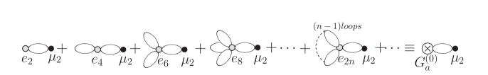
Figure 2: The sum of all connected first-order graphs consisting of $e_{2n}$-vertices and the $\mu$-vertex.

In Fig.2, an $e_{2n}$-$\mu$ graph has a factor ${\frac{(2n)!}{(n-1)!(2!)^{(n-1)}}}$. The sum in Fig.2, $G_{a,I}^{(1)}$, has the following result

$$G_{a,I}^{(1)} = -\sum_{n=1}^{\infty}(f_{00}^{-1})^{n-1}e^{4\pi a^{2}I_{(1)}({\cal M}^{2})}{\frac{(i\sqrt{8\pi}a)^{2n}}{(2n)!}}\int d^{\nu}\vec{r}_{1}(f^{-1}_{0\vec{r}_{1}})^{2}(-{\frac{1}{2}}\mu^{2})\cdot{\frac{(2n)!}{(n-1)!(2!)^{n-1}}}$$ (47)

$$= {\frac{1}{2}}\mu^{2}(i\sqrt{8\pi}a)^{2}\int d^{\nu}\vec{r}_{1}(f^{-1}_{0\vec{r}_{1}})^{2}G_{a}^{(0)}\;.$$

Note that at the first order of $\epsilon$, there is an additional total factor ${\frac{(-1)^{1}}{1}}$ the expansion factor, and we have added it to Eq.(46). We do so in the later Eq.(47), too.

Comparing the result Eq.(46) with Fig.2, one can see that the sum of all possible connected graphs consisting of the $e_{2n}$-vertices and the $\mu$-vertex amounts to the sum of all graphs consisting of an external $2$-leg vertex with a coefficient ${\frac{(i\sqrt{8\pi}a)^{2}}{2!}}G_{a}^{(0)}$ (the vertex represented by the cross-centered circle with two legs in the right hand side of Fig.2) and the $\mu$-vertex (in fact, only two of such graphs). Noting that the $\mu$-vertex has two legs, one would admit that the sum of all possible connected graphs consisting of external vertices and an $n$-leg internal vertex amounts to the sum of all graphs consisting of an external $n$-leg vertex with a coefficient ${\frac{(i\sqrt{8\pi}a)^{n}}{n!}}G_{a}^{(0)}$ (we will call it an external $n$-leg exponential vertex) and the $n$-leg internal vertex (one can prove it directly in the way of getting to Eq.(46)). Similarly to those in Fig.1 and Fig.2, we will graphically represent an external $n$-leg exponential vertex by a cross-centered circle with $n$ legs. Furthermore, one can also check that the sum of all connected graphs which consist of $C_{2n}$-vertices and some external or internal $2n$-leg vertex amounts to summing up all connected graphs which are made by an internal $2n$-leg vertex with a coefficient $-2\Omega{\frac{(i\sqrt{8\pi}\beta)^{2n}}{(2n)!}}e^{-4\pi\beta^{2}{\cal U}}$ (we will call it an internal $2n$-leg cosine vertex) and the external or internal $2n$-leg vertex. We will graphically represent the internal $2n$-leg cosine vertex by a dot-centered circle with $2n$ legs.

From the analysis and results in last paragraph, the sum of all $e_{2n}$-$C_{2n}$ graphs can be depicted in Fig.3.

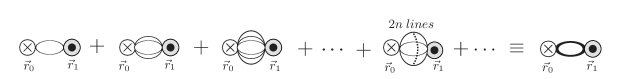
Figure 3: The sum of all connected first-order graphs consisting of $e_{2n}$-vertices and the $C_{2n}$-vertices.

In Fig.3, $\vec{r}_{0}=0$ and a $2n$-line graph has a factor $(2n)!$. Note that in the right hand side of Fig.3, we have used the graph with two bold lines to represent the sum of all possible graphs with even lines between two vertices. Thus, the sum in Fig.3, $G_{a,II}^{(1)}$, can be calculated as

$$G_{a,II}^{(1)} = 2\Omega e^{-4\pi\beta^{2}{\cal U}}G_{a}^{(0)}\int d^{\nu}\vec{r}_{1}\sum^{\infty}_{n=1}{\frac{(i\sqrt{8\pi}a)^{2n}}{(2n)!}}(f^{-1}_{0\vec{r}_{1}})^{2n}{\frac{(i\sqrt{8\pi}\beta)^{2n}}{(2n)!}}\cdot(2n)!$$ (48)

$$= 2\Omega e^{-4\pi(a^{2}+\beta^{2}){\cal U}}\int d^{\nu}\vec{r}_{1}[\cosh(8\pi a\beta f^{-1}_{0\vec{r}_{1}})-1]\;.$$

Comparing last equation and the right hand side of Fig.3, one see that the two bold lines corresponds to the integrand $[\cosh(8\pi a\beta f^{-1}_{0\vec{r}_{1}})-1]$ and the factor before the integral in Eq.(47) comes from the $n$-independent parts of the coefficients for the external $2n$-leg exponential and internal $2n$-leg cosine vertices. It is evident that summing up $G_{a,I}^{(1)}$ in Eq.(46) and $G_{a,II}^{(1)}$ in Eq.(47) gives rise to Eq.(35).

At the second order, diagrams will be complicated. There exist nine types of graphs: two types for one $e_{2n}$ vertex connecting with two $\mu$-vertices (figures (a) and (b) in Fig.4), four types for one $e_{2n}$ vertex connecting with two $C_{2n}$-vertices (figures (f), (g), (h) and (i) in Fig.4), and three types for connections among one $e_{2n}$ vertex, one $\mu$-vertex and one $C_{2n}$-vertex (figures (c), (d) and (e) in Fig.4). The sum of every type of graphs is depicted in Fig.4.

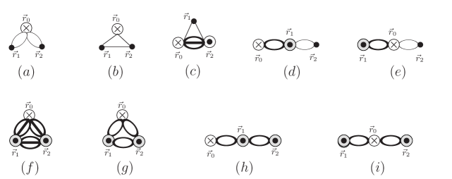
Figure 4: The sum of all connected second-order graphs consisting of $e_{2n}$-, $C_{2n}$-vertices and $\mu$-vertex.

In Fig.4, the graph with three bold lines between two vertices represents the sum of all similar graphs with odd lines between the same two vertices, and a set of three bold lines corresponds to a negative hyperbolic sine function (one can check it by doing as was done in Eq.(47)). The results of graphs in Fig.4 can be calculated as follow, respectively. The graph $(a)$ in Fig.4 is simply

$$G_{a,a}^{(2)} = {\frac{1}{2}}{\frac{(i\sqrt{8\pi}a)^{4}}{4!}}G_{a}^{(0)}\int d^{\nu}\vec{r}_{1}\int d^{\nu}\vec{r}_{2}(f^{-1}_{0\vec{r}_{1}})^{2}(f^{-1}_{0\vec{r}_{2}})^{2}(-{\frac{1}{2}}\mu^{2})(-{\frac{1}{2}}\mu^{2})\cdot C_{4}^{2}\cdot 2\cdot 2$$ (49)

$$= 8\pi^{2}a^{4}\mu^{4}e^{-4\pi a^{2}{\cal U}}\int d^{\nu}\vec{r}_{1}\int d^{\nu}\vec{r}_{2}(f^{-1}_{0\vec{r}_{1}})^{2}(f^{-1}_{0\vec{r}_{2}})^{2}$$

In Eq.(48), the symbol $C_{4}^{2}$ is a number of combinations, and we have added the factor ${\frac{1}{2}}$ which is the total factor at the second order. We also do so for the other second-order graphs. The graph $(b)$, $(c)$, $(d)$, $(e)$, $(f)$, $(g)$, $(h)$ and $(i)$ in Fig.4 can be written as

$$G_{a,b}^{(2)} = {\frac{1}{2}}{\frac{(i\sqrt{8\pi}a)^{2}}{2!}}G_{a}^{(0)}\int d^{\nu}\vec{r}_{1}\int d^{\nu}\vec{r}_{2}f^{-1}_{0\vec{r}_{1}}f^{-1}_{0\vec{r}_{2}}f^{-1}_{\vec{r}_{1}\vec{r}_{2}}(-{\frac{1}{2}}\mu^{2})(-{\frac{1}{2}}\mu^{2})\cdot C_{2}^{1}\cdot 2\cdot 2$$ (50)

$$= -4\pi a^{2}\mu^{4}e^{-4\pi a^{2}{\cal U}}\int d^{\nu}\vec{r}_{1}\int d^{\nu}\vec{r}_{2}f^{-1}_{0\vec{r}_{1}}f^{-1}_{0\vec{r}_{2}}f^{-1}_{\vec{r}_{1}\vec{r}_{2}}\;,$$

$$G_{a,c}^{(2)} = {\frac{1}{2}}{\frac{(i\sqrt{8\pi}a)^{1}}{1!}}G_{a}^{(0)}\int d^{\nu}\vec{r}_{1}\int d^{\nu}\vec{r}_{2}f^{-1}_{0\vec{r}_{1}}f^{-1}_{\vec{r}_{1}\vec{r}_{2}}\{-\sinh[8\pi a\beta f^{-1}_{0\vec{r}_{2}}]\}$$ (51)

$$\hskip 56.9055pt\times(-{\frac{1}{2}}\mu^{2})(-2\Omega){\frac{(i\sqrt{8\pi}\beta)^{1}}{1!}}e^{-4\pi\beta^{2}{\cal U}}\cdot 2\cdot 2$$

$$= 16\pi a\beta\mu^{2}\Omega e^{-4\pi(a^{2}+\beta^{2}){\cal U}}\int d^{\nu}\vec{r}_{1}\int d^{\nu}\vec{r}_{2}f^{-1}_{0\vec{r}_{1}}f^{-1}_{\vec{r}_{1}\vec{r}_{2}}\sinh[8\pi a\beta f^{-1}_{0\vec{r}_{2}}]\;,\hskip 56.9055pt$$

$$G_{a,d}^{(2)} = {\frac{1}{2}}G_{a}^{(0)}\int d^{\nu}\vec{r}_{1}\int d^{\nu}\vec{r}_{2}[\cosh(8\pi a\beta f^{-1}_{0\vec{r}_{1}})-1]$$ (52)

$$\hskip 56.9055pt\times(-2\Omega){\frac{(i\sqrt{8\pi}\beta)^{2}}{2!}}e^{-4\pi\beta^{2}{\cal U}}(f^{-1}_{\vec{r}_{1}\vec{r}_{2}})^{2}(-{\frac{1}{2}}\mu^{2})\cdot 2\cdot 2$$

$$= -8\pi\beta^{2}\mu^{2}\Omega e^{-4\pi(a^{2}+\beta^{2}){\cal U}}\int d^{\nu}\vec{r}_{1}\int d^{\nu}\vec{r}_{2}(f^{-1}_{\vec{r}_{1}\vec{r}_{2}})^{2}[\cosh(8\pi a\beta f^{-1}_{0\vec{r}_{1}})-1]\;,\hskip 56.9055pt$$

$$G_{a,e}^{(2)} = {\frac{1}{2}}\int d^{\nu}\vec{r}_{1}\int d^{\nu}\vec{r}_{2}(-2\Omega)e^{-4\pi\beta^{2}{\cal U}}[\cosh(8\pi a\beta f^{-1}_{0\vec{r}_{1}})-1]$$ (53)

$$\hskip 56.9055pt\times G_{a}^{(0)}{\frac{(i\sqrt{8\pi}a)^{2}}{2!}}(f^{-1}_{0\vec{r}_{2}})^{2}(-{\frac{1}{2}}\mu^{2})\cdot 2\cdot 2$$

$$= -8\pi a^{2}\mu^{2}\Omega e^{-4\pi(a^{2}+\beta^{2}){\cal U}}\int d^{\nu}\vec{r}_{1}\int d^{\nu}\vec{r}_{2}(f^{-1}_{0\vec{r}_{2}})^{2}[\cosh(8\pi a\beta f^{-1}_{0\vec{r}_{1}})-1]\;,\hskip 42.67912pt$$

$$G_{a,f}^{(2)} = {\frac{1}{2}}G_{a}^{(0)}\int d^{\nu}\vec{r}_{1}\int d^{\nu}\vec{r}_{2}(-2\Omega)e^{-4\pi\beta^{2}{\cal U}}[-\sinh(8\pi a\beta f^{-1}_{0\vec{r}_{1}})]\hskip 113.81102pt$$ (54)

$$\hskip 56.9055pt\times(-2\Omega)e^{-4\pi\beta^{2}{\cal U}}[-\sinh(8\pi a\beta f^{-1}_{0\vec{r}_{2}})][-\sinh(8\pi\beta^{2}f^{-1}_{\vec{r}_{1}\vec{r}_{2}})]$$

$$= -2\Omega^{2}e^{-4\pi(a^{2}+2\beta^{2}){\cal U}}\int d^{\nu}\vec{r}_{1}\int d^{\nu}\vec{r}_{2}\sinh(8\pi a\beta f^{-1}_{0\vec{r}_{1}})$$

$$\hskip 85.35826pt\times\sinh(8\pi a\beta f^{-1}_{0\vec{r}_{2}})\sinh(8\pi\beta^{2}f^{-1}_{\vec{r}_{1}\vec{r}_{2}})\;,\hskip 56.9055pt$$

$$G_{a,g}^{(2)} = {\frac{1}{2}}G_{a}^{(0)}\int d^{\nu}\vec{r}_{1}\int d^{\nu}\vec{r}_{2}(-2\Omega)e^{-4\pi\beta^{2}{\cal U}}[\cosh(8\pi a\beta f^{-1}_{0\vec{r}_{1}})-1]\hskip 113.81102pt$$ (55)

$$\hskip 56.9055pt\times(-2\Omega)e^{-4\pi\beta^{2}{\cal U}}[\cosh(8\pi a\beta f^{-1}_{0\vec{r}_{2}})-1][\cosh(8\pi\beta^{2}f^{-1}_{\vec{r}_{1}\vec{r}_{2}})-1]$$

$$= 2\Omega^{2}e^{-4\pi(a^{2}+2\beta^{2}){\cal U}}\int d^{\nu}\vec{r}_{1}\int d^{\nu}\vec{r}_{2}[\cosh(8\pi a\beta f^{-1}_{0\vec{r}_{1}})-1]$$

$$\hskip 56.9055pt\times[\cosh(8\pi a\beta f^{-1}_{0\vec{r}_{2}})-1][\cosh(8\pi\beta^{2}f^{-1}_{\vec{r}_{1}\vec{r}_{2}})-1]\;,\hskip 56.9055pt$$

$$G_{a,h}^{(2)} = {\frac{1}{2}}G_{a}^{(0)}\int d^{\nu}\vec{r}_{1}\int d^{\nu}\vec{r}_{2}(-2\Omega)e^{-4\pi\beta^{2}{\cal U}}[\cosh(8\pi a\beta f^{-1}_{0\vec{r}_{1}})-1]$$ (56)

$$\hskip 170.71652pt\times(-2\Omega)e^{-4\pi\beta^{2}{\cal U}}[\cosh(8\pi\beta^{2}f^{-1}_{\vec{r}_{1}\vec{r}_{2}})-1]$$

$$= 2\Omega^{2}e^{-4\pi(a^{2}+2\beta^{2}){\cal U}}\int d^{\nu}\vec{r}_{1}\int d^{\nu}\vec{r}_{2}[\cosh(8\pi a\beta f^{-1}_{0\vec{r}_{1}})-1]$$

$$\hskip 170.71652pt\times[\cosh(8\pi\beta^{2}f^{-1}_{\vec{r}_{1}\vec{r}_{2}})-1]\;,\hskip 62.59596pt$$

$$G_{a,i}^{(2)} = {\frac{1}{2}}\int d^{\nu}\vec{r}_{1}\int d^{\nu}\vec{r}_{2}(-2\Omega)e^{-4\pi\beta^{2}{\cal U}}[\cosh(8\pi a\beta f^{-1}_{0\vec{r}_{1}})-1]$$ (57)

$$\hskip 113.81102pt\times G_{a}^{(0)}(-2\Omega)e^{-4\pi\beta^{2}{\cal U}}[\cosh(8\pi a\beta f^{-1}_{0\vec{r}_{2}})-1]$$

$$= 2\Omega^{2}e^{-4\pi(a^{2}+2\beta^{2}){\cal U}}\{\int d^{\nu}\vec{r}_{1}[\cosh(8\pi a\beta f^{-1}_{0\vec{r}_{1}})-1]\}^{2}\;.\hskip 113.81102pt$$

For easily reading, every first expression in Eqs.(48)—(56) was written down in the way of one factor in the expression corresponding to one part in the relevant graph (some graphs have symmetrical factors). One can check that the sum of Eqs.(48)—(56) coincides with Eq.(39). Thus, one has seen that the VP expansion of one-point functions can be performed by borrowing Feynman diagrammatic technique in conventional perturbative theory.

IV sG and shG Field Theories with $\nu=2$: One-order VP Results

Subsection A and B will provide comparisons of the one-order VP results for sG and shG field theories with the conjectured exact results, respectively, and subsection C will compare the one-order VP results with the one-order perturbative results sG field theories .

IV.1 Comparisons with the Conjectured Results: sG Field Theory

In two-dimensional Euclidean space, Eqs.(32) and (35) give ($\epsilon=1$)

$$G_{a}^{I} = ({\frac{\mu^{2}}{{\cal M}^{2}}})^{a^{2}}-4\pi\mu^{2}a^{2}({\frac{\mu^{2}}{{\cal M}^{2}}})^{a^{2}}\int d^{2}\vec{r}_{1}(f^{-1}_{0\vec{r}_{1}})^{2}$$

$$\ \ \ \ \ +2\Omega({\frac{\mu^{2}}{{\cal M}^{2}}})^{a^{2}+\beta^{2}}\sum_{n=1}^{\infty}{\frac{(8\pi a\beta)^{2n}}{(2n)!}}\int d^{2}\vec{r}_{1}(f^{-1}_{0\vec{r}_{1}})^{2n}$$

$$\hskip 42.67912pt=({\frac{\mu^{2}}{{\cal M}^{2}}})^{a^{2}}(1-2a^{2}K_{02})+4\pi{\frac{\Omega}{{\cal M}^{2}}}({\frac{\mu^{2}}{{\cal M}^{2}}})^{a^{2}+\beta^{2}-1}K_{0c}\;,$$ (58)

where,

$$K_{02}\equiv\int^{\infty}_{0}dxxK_{0}^{2}(x),\ \ \ \ \ \ \ \ K_{0c}\equiv\int^{\infty}_{0}dxx[\cosh(4a\beta K_{0}(x))-1].$$

To determine the auxiliary parameter $\mu$, as stated in Sect. II, we can require that ${\frac{dG_{a}^{I}}{d(\mu^{2})}}=0$ according to the PMS, and have

$${\frac{\mu^{2}}{{\cal M}^{2}}}=\biggl{(}4\pi{\frac{\Omega}{{\cal M}^{2}}}K_{0c}{\frac{1-a^{2}-\beta^{2}}{a^{2}(1-2a^{2}K_{02})}}\biggl{)}^{1/(1-\beta^{2})}\;.$$ (59)

Thus, Eq.(57) with Eq.(58) gives $G_{a}^{I}$, the approximate result of $G_{a}$ up to the first order in the VP theory. Note that the normal-ordering parameter ${\cal M}$ can be taken as any positive value with mass dimension, and different choice of its value leads to just a finite multiplicative redefinition of $\Omega$ 25 (1975). Once ${\cal M}$ is chosen, the theory is defined and the parameter $\Omega$ is given a precise meaning, just as the choice of the normalization of the field $\cos(\beta\phi)$ in Ref. 4 does. We will take ${\cal M}$ as unit. This choice renders every quantities in Eqs.(57) and (58) dimensionless, and simultaneously amounts to taking the same normalization conditions as Eqs.(6) and (16) in Ref. 4 . The latter point can be checked by directly calculating the relevant two-point correlation function with the two points approaching each other within our formalism and then comparing the result with that in Ref. 4 . Thus, our results can be compared with the exact formula. Because being exponential-like interaction, the $two$-dimensional sG field theory can be rendered finite only for the case $\beta^{2}<{\frac{1}{2}}$ by the Coleman’s normal-ordering prescription (it amounts to the renormalization of the mass parameter. For the range of $\beta$ where the sG field theory diverges, one has to resort to a further renormalization procedure), and accordingly $G_{a}$ is finite for the case $\beta^{2}<{\frac{1}{2}}$ and $a\beta<{\frac{1}{2}}$. And so $G_{a}^{I}$ here is finite only for the range $a\beta<{\frac{1}{2}}$ (one can see it by noticing the integral $K_{0c}$). Fortunately, this range of $\beta$ is just the validity scope of the conjectured exact formula in Ref. 4 . Numerically, $G^{I}_{a}$ can be given with Mathematica programme for the range of $\alpha\beta<0.426925$, as stated in Ref. 27 . This also occurs at the shG field theory.

Now we consider the comparison for the sG field theory. From Eq.(12) in Ref. 4 , the dimensionless $\Omega$ can be written as

$$\Omega={\frac{\Gamma(\beta^{2})}{\pi\Gamma(1-\beta^{2})}}\biggl{[}{\frac{\sqrt{\pi}\Gamma({\frac{1}{2}}+{\frac{\xi}{2}})}{2\Gamma({\frac{\xi}{2}})}}\biggl{]}^{2-2\beta^{2}}$$ (60)

with $\xi={\frac{\beta^{2}}{1-\beta^{2}}}$. In last equation, we took the soliton mass as unit to make $\Omega$ dimensionless. For the conjectured exact formula Eq.(20) in Ref. 4 , we also do so and have

$$G_{a}^{exact} = {\frac{2\sin({\frac{\pi\xi}{2}})\Gamma({\frac{1}{2}}+{\frac{\xi}{2}})\Gamma(1-{\frac{\xi}{2}})}{4\sqrt{\pi}}}$$ (61)

$$\hskip 28.45274pt\exp\{\int^{\infty}_{0}{\frac{dt}{t}}[{\frac{\sinh^{2}(2a\beta t)}{2\sinh(\beta^{2}t)\sinh(t)\cosh((1-\beta^{2})t)}}-2a^{2}e^{-2t}]\}\;.$$

To compare $G_{a}^{I}$ with the conjectured exact result, we depict $G_{a}^{I}$ according to Eq.(57) with Eqs.(58) and (59) as the left figure of Fig.5, and the exact result $G^{exact}_{a}$ according to Eq.(60) as the right figure of Fig.5.

Figure 5: Comparison of $G_{a}^{I}$ (the left) with the conjectured exact result $G_{a}^{exact}$ (the right).

In Fig.5, the parameter range is $0\leq a<0.65$ and $0\leq\beta<0.65$. In principle, the two figures in Fig.5 can be extended to all range $\alpha\beta<0.5$. From Fig.5, one can see that for smaller $\beta$ and larger $a$, $G_{a}$ tends to zero, and for larger $\beta$ and $a$, $G_{a}$ is greater than the value $1$. When a large $\beta$ is given, $G_{a}$ increases with the increase of $a$, and when a small $\beta$ is given, $G_{a}$ decreases with the increase of $a$. On the other hand, the two figures in Fig.5 resemble each other very well and suggest that for the range of the parameter $\{a,\beta\}$ drawn in Fig.5 $G_{a}^{I}$ has a good agreement with the conjectured exact result. Our numerical analysis indicates that for the case of $a<0.2$ or so, the one-order results almost completely agree with the conjectured exact results, and for larger $a$, our results differ from the exact results with about ten percents or so (at most with 20 more percents when $a$ approaches values with $a\beta\leq 0.426925$ satisfied, see Table I in Ref. 27 ).

Figure 6: Comparison between the one-order ($G_{a}^{I}$, solid curve) and conjectured exact ($G_{a}^{exact}$, dotted curve) sG VEVs of exponential fields at $\beta=0.15$. The dashed curve is the one-order perturbative result ($G_{a}^{Ipert}$, see subsection C) at the same value of $\beta$. At this value of $\beta$,$G_{a}^{Ipert}$ and $G_{a}^{exact}$ are widely discrepant.

Figure 7: Similar to Fig.6 but at $\beta=0.7$. At this case, the one-order perturbative result (the dashed curve) is almost coincident with the conjectured exact result.

For a concrete illustration, we draw $G_{a}^{I}$ (the solid curves) and the exact result $G_{a}^{exact}$ (the dotted curves) at $\beta=0.15$ and $0.7$ in Fig.6 and Fig.7, respectively (the dashed curves is the perturbative results, see next subsection C). These two figures indicate that $G_{a}^{I}$ is always greater than $G_{a}^{exact}$.

IV.2 Comparisons with the Conjectured Results: shG Field Theory

In the Euclidean space, the shG Lagrangian density is

$${\cal L}_{shG}={\frac{1}{2}}\nabla_{\vec{r}}\phi_{\vec{r}}\nabla_{\vec{r}}\phi_{\vec{r}}+2\Delta\cosh(\sqrt{8\pi}\gamma\phi_{\vec{r}})\;.$$ (62)

For the convenience of comparison with the conjectured exact VEV of the exponential field in the shG field theory in Ref. 5 , here we are interested in the VEV $G_{b}\equiv<e^{\sqrt{8\pi}b\phi(0)}>$. Taking $a=-ib$, $\beta=i\gamma$ and $\Omega=-\Delta$ in Eq.(57), we get the one-order VP approximate result of $G_{b}$, $G_{b}^{I}$, as follows

$$G_{b}^{I}=(\mu^{2})^{-b^{2}}(1+2b^{2}K_{02})-4\pi\Delta(\mu^{2})^{-b^{2}-\gamma^{2}-1}K_{0ch}$$ (63)

with the parameter $\mu^{2}$ satisfied

$$\mu^{2}=\biggl{(}4\pi\Delta K_{0ch}{\frac{1+b^{2}+\gamma^{2}}{b^{2}(1+2b^{2}K_{02})}}\biggl{)}^{1/(1+\gamma^{2})}\;,$$ (64)

where, $K_{0ch}\equiv\int^{\infty}_{0}dxx[\cosh(4b\gamma K_{0}(x))-1]$ is similar to $K_{0c}$. From Eqs.(9) and (8) in Ref. 5 , the dimensionless $\Delta$ has the following form

$$\Delta=-{\frac{\Gamma(-\gamma^{2})}{\pi\Gamma(1+\gamma^{2})}}\biggl{[}{\frac{\Gamma({\frac{1}{(2+2\gamma^{2})}})\Gamma(1+{\frac{\gamma^{2}}{2+2\gamma^{2}}})}{4\sqrt{\pi}}}\biggl{]}^{2+2\gamma^{2}}\;,$$ (65)

and the dimensionless conjectured exact expression of $G_{b}$, $G_{b}^{exact}$, is

$$G_{b}^{exact} = \biggl{[}{\frac{\Gamma({\frac{1}{(2+2\gamma^{2})}})\Gamma(1+{\frac{\gamma^{2}}{2+2\gamma^{2}}})}{4\sqrt{\pi}}}\biggl{]}^{-2b^{2}}$$ (66)

$$\hskip 28.45274pt\exp\Bigl{\{}\int^{\infty}_{0}{\frac{dt}{t}}\bigl{[}{\frac{\sinh^{2}(2b\gamma t)}{2\sinh(\gamma^{2}t)\sinh(t)\cosh((1+\gamma^{2})t)}}+2b^{2}e^{-2t}\bigl{]}\Bigl{\}}\;.$$

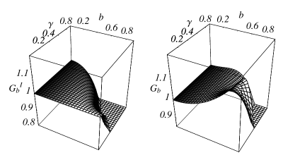
Figure 8: Comparison of $G_{b}^{I}$ with the conjectured exact $G_{b}$.

In Eqs.(64) and (65), we adopted symbols here and took the particle mass as unit. Now we can compare $G_{b}^{I}$ with $G_{b}^{exact}$. We depict $G_{b}^{I}$ (the left figure) and $G_{b}^{exact}$ (the right figure) in Fig.8 for the range of $b<0.9$ and $\gamma<0.9$ (it can be extended to the all tractable range of $b\gamma<0.426925$ ). In the left figure of Fig.8, $G_{b}^{I}$ is set to zero for the range of $b\gamma>0.426925$ where Mathematica couldn’t produce finite numerical results. The two surfaces in Fig.8 are basically resemble each other, except for the cases of larger $b$ and simultaneously smaller $\gamma$. Numerical analysis indicates that for a given value of $\beta$, $G_{b}^{I}$ always decreases with the increase of $b$, while $G_{b}^{exact}$ is first increase and then goes down with the increase of $b$. But, for not large $b$, the relative differences of $G_{b}^{I}$ from the conjectured exact result $G_{b}^{exact}$ are small, the situations on the differences between $G_{b}^{I}$ and $G_{b}^{exact}$ are analogous to those for the sG field theory.

Figure 9: Comparison of $G_{b}^{I}$ (solid) with the conjectured exact $G_{b}$ (dotted) at $\gamma=0.2$.

Figure 10: Comparison of $G_{b}^{I}$ (solid) with the conjectured exact $G_{b}$ (dotted) at $\gamma=0.8$.

We show these points in Fig.9 and Fig.10 for the values of $\gamma=0.2$ and $\gamma=0.8$, respectively. In Figs.9 and 10, the dotted curves are for $G_{b}^{exact}$ and the solid ones for $G_{b}^{I}$. Specially, when $b$ is smaller than $0.2$ or so, $G_{b}^{I}$ almost completely coincides with the conjectured result $G_{b}^{exact}$. These two figures show that for the shG field theory, $G_{b}^{I}$ is always smaller than $G_{b}^{exact}$, which is opposite to that for the sG field theory.

By the way, if we choose $\Delta$ as unit instead of setting the particle mass as unit as did in the above, then the numerical analysis indicates that the dependence of $G_{b}^{I}$ upon $b$ at a given $\beta$ is qualitatively similar to that of $G_{b}^{exact}$.

IV.3 Comparisons with the One-order Perturbative Results: sG Field Theory

Using the massive Thirring model, Ref. 12 (Poghossian) calculated $G_{a}$ perturbatively up to the first order of the coupling $g$, and obtained

$$G_{a}^{Ipert} = ({\frac{1}{2}})^{2a^{2}}\exp\{\int^{\infty}_{0}{\frac{dt}{t}}[{\frac{\sinh^{2}(\sqrt{2}at)}{\sinh^{2}(t)}}-2a^{2}e^{-2t}]\}$$ (67)

$$\hskip 28.45274pt\times[1+{\frac{g}{8\pi}}[-2\Psi({\frac{1}{2}})+8a^{2}(1-4\log 2)+8a^{2}(\Psi(\sqrt{2}a)+\Psi(-\sqrt{2}a))$$

$$\hskip 56.9055pt+(1-8a^{2})(\Psi({\frac{1+2\sqrt{2}a}{2}})+\Psi({\frac{1-2\sqrt{2}a}{2}}))]]+o(g^{2})\;,$$

where, the coupling $g$ is related to the sG coupling $\beta$ as follows

$${\frac{g}{\pi}}={\frac{1}{2\beta^{2}}}-1\,.$$ (68)

Eq.(67) indicates that $g\to 0$ corresponds to $\beta^{2}\to{\frac{1}{2}}$.

Figure 11: Similar to Fig.6 and Fig.7, but at $\beta=0.65$.

In Fig.11, we compare the one-order perturbative (the dashed curves) and VP (solid) results with the conjectured exact results (dotted) at the case of $\beta=0.65$. In subsection A of this section, the same comparisons were made at $\beta=0.15$ and $0.7$ in Fig.6 and Fig.7, respectively. In Figs.7, $\beta^{2}=0.49$, $i.e.$, $\beta$ approaches ${\frac{1}{2}}$ or $g\to 0$, the one-order perturbative results are almost completely identical to the conjectured exact results for all the plotted values of $a$, while the one-order VP results have evident differences (the relative errors are 20% or so at most) from the conjectured exact results for larger values of $a$. In Fig.11, $\beta^{2}\approx 0.42$, the one-order perturbative results (dashed) have quite large deviations from the conjectured exact results (dotted) for larger values of $a$, and differences of the one-order VP results (solid) from the conjectured exact results for larger values of $a$ get smaller than the case of $\beta^{2}=0.49$. In Fig.6, $\beta^{2}=0.02$, the one-order perturbative results and the conjectured exact results are widely discrepant for all the plotted values of $a$, while differences of the one-order VP results from the conjectured exact results for larger values of $a$ get much smaller than the cases of $\beta^{2}=0.49$ and $0.42$. Besides, in Figs. 6, 7, and 11, the one-order VP results almost coincide with the conjectured exact results for not large $a$ ($<0.2$ or so). To illustrate the dependency of the deviations of the one-order perturbative and VP results from the conjectured exact results upon the coupling $\beta$, $G_{a}^{Ipert}$, $G_{a}^{I}$ and $G_{a}^{exact}$ with $a=0.2,0.3$ and $0.5$ are depicted as functions of $\beta$ in Figs.12, 13 and 14, respectively.

Figure 12: The dependances of $G_{a}^{Ipert}$(dashed), $G_{a}^{I}$(solid) and $G_{a}^{exact}$(dotted) upon $\beta$ for $a=0.2$.

Figure 13: The dependances of $G_{a}^{Ipert}$(dashed), $G_{a}^{I}$(solid) and $G_{a}^{exact}$(dotted) upon $\beta$ for $a=0.3$.

Figure 14: The dependances of $G_{a}^{Ipert}$(dashed), $G_{a}^{I}$(solid) and $G_{a}^{exact}$(dotted) upon $\beta$ for $a=0.5$.

These three figures evidently show that the one-order perturbative results (dashed) have good agreements with the conjectured exact results (dotted) only when $\beta^{2}$ approaches the value ${\frac{1}{2}}$ ($i.e.,$ when $g\to 0$), but their deviations from the conjectured exact results appear, for a given value of $a$ (not too small), and become larger and larger when $\beta^{2}$ decreases from ${\frac{1}{2}}$. For a given $a$, when values of $\beta^{2}$ is much smaller than ${\frac{1}{2}}$, the one-order perturbative and conjectured exact results are widely discrepant. On the other hand, the one-order VP results (solid) are almost identical to the conjectured exact results for not large values of $\beta$, and have not too larger differences from the conjectured exact results even when $\beta^{2}$ approaches ${\frac{1}{2}}$.

V Conclusion

In this paper, we developed a VP scheme to calculate the VEVs of local fields in relativistical QFTs. For a class of scalar field theories whose potential have Fourier representations, we obtained the Gaussian smearing formulae for the VEVs of a comparatively general local field. As an application and illustrations on the scheme and the Gaussian smearing formulae, we considered the sG and shG field theories. This application provided an example in both directly and Feynman-diagrammatically performing the VP scheme, and showed the usefulness of the Gaussian smearing formulae. The Gaussian smearing formulae can relieve us of hard labor in path integrals. The usefulness of the Gaussian smearing formulae can also be envisioned from the smearing formulae for the higher order effective classical potential in statistical mechanics 38 , which succeeded in applying to the singular Coulomb potential. Additionally, according to the saying in Ref. 2 when discussing normal-ordering prescription, the existence of the Fourier representation of a given $V(\phi)$ for the validity of the Gaussian smearing formulae is irrelevant in the derivation of section II, because the final Gaussian smearing formulae are purely algebraic 2 . Although the one-order VP results are the lowest approximate in VP theory, the numerical discussions in last section indicated that the one-order VP VEVs of the exponential fields for the sG and shG field theories give a strong support to the conjectured formulae on the exact VEVs in Refs. 4 ; 5 and the first paper in Ref. 6 , at least, for not large values of the coupling and the exponential-field parameter. They also suggest the effectiveness of the VP scheme here in calculating the VEVs of local fields for QFTs. The comparisons in last section also illustrates the non-perturbability of the VPT scheme here and its advantages over the perturbative theory. We believe that the VP scheme in the present paper can provide an effective, systematical controllable non-perturbative approximate tool for calculating VEVs of local fields in relativistic QFTs.

As was pointed out in Ref. 27 , there exist some interesting problems based on our work, and here we do not repeat them one by one. Nevertheless, we intend to stress that a further investigation on the higher order results would improve the one-order VP results here and show the convergency of the VP theory. As a matter of fact, a numerical analysis on the VP results up to the second order in the sG field theory in Ref. 27 has suggested this point. The applications of the scheme in the present paper to other field theories maybe also give a good check and substantial support to the other existed conjectured exact formulae 5 ; 6 ; 7 ; 8 ; 9 ; 10 ; 11 ; 12 . Simultaneously, the problem of calculating VEVs of local fields provides a good laboratory for the VP theory because there existed so many conjectures on VEVs of local fields in various perturbed conformal field theories. Of course, generalizing the VP scheme here to other physical problems will be interesting and useful. For example, the bound state problems in relativistic QFT is a notoriously difficult non-perturbative problems, and we noticed that there had existed an approach of attacking it which is a combination of variational method and perturbative theory 41 . The approach in Ref. 41 can be regarded as a method of calculating VEV, but, as pointed by the authors, it is valid only for the weak coupling, because the variational procedure in it is to choose the appropriate two-particle operator and the expansion scheme is a naive perturbative expansion. We think that based on the work in this reference, the VP scheme here can be generalized for calculating bound-state mass, and this generalization will be meaningful and interesting.

- (1) A. Patashinskii, V. Pokrovskii, Fluctuation Theory of Phase Transitions (Pergamon Press, Oxford, 1979); A. M. Tsvelik, Quantum Field Theory in Condensed Matter Physics (Cambridge University Press, Cambridge,1995).
- (2) Jean Zinn-Justin, Quantum Field theory and Critical Phenomena, 4th Edition (Clarendon Press, Oxford, 2002).
- (3) V.A. Fateev, Phys. Lett. B 324, 45(1994); Al. Zamolodchikov, Int. J. Mod. Phys. A 10, 1125(1995).
- (4) S. Lukyanov and A. Zamolodchikov, Nucl. Phys. B 493, 571(1997).
- (5) V. Fateev, S. Lukyanov, A. Zamolodchikov and Al. Zamolodchikov, Phys. Lett. B 406, 83(1997).
- (6) V. Fateev, S. Lukyanov, A. Zamolodchikov and Al. Zamolodchikov, Nucl. Phys. B 516, 652(1998); P. Baseilhac and V. Fateev, Nucl. Phys. B 532, 567(1998); V. A. Fateev, Mod. Phys. Lett. A 15, 259(2000); P. Baseilhac, M. Stanishkov, Nucl. Phys. B 612, 373(2001); P. Baseilhac, M. Stanishkov, Phys. Lett. B 554, 217(2003).
- (7) V. Fateev, D. Fradkin, S. Lukyanov, A. Zamolodchikov, Al. Zamolodchikov, Nucl. Phys. B 540, 587(1999); C. R. Ahn, P. Baseilhac, V.A. Fateev, C. J. Kim, C. H. Rim, Physics Letters B 481, 114(2000); C. R. Ahn, C. J. Kim and C. H. Rim, J. Stat. Phys. 102, 385(2001); V. A. Fateev, Mod. Phys. Lett. A 16, 1201(2001); P. Baseilhac, Nucl. Phys. B 636, 465(2002).
- (8) P. Baseilhac, Nucl. Phys. B 594, 607(2001).
- (9) V. Fateev, A. Zamolodchikov, Al. Zamolodchikov, Boundary Liouville field theory I. Boundary state and boundary two-point function, hep-th/0001012; A. Zamolodchikov, Al. Zamolodchikov, Liouville field theory on a pseudosphere, hep-th/0101152; C. R. Ahn, C. H. Rim, M. Stanishkov, Nucl. Phys. B 636, 497(2002); T. Fukuda, K. Hosomichi, Nucl. Phys. B 635, 215(2002).
- (10) C. R. Ahn, M. Stanishkov and M. Yamamoto, Nucl. Phys. B 683, 177(2004); J. McGreevy, S. Murthy and H. Verlinde, J. High Energy Phys. 04, 015(2004).
- (11) P.E. Dorey , M. Pillin , R. Tateo, G.M.T. Watts, Nucl. Phys. B 594, 625(2001).
- (12) V. V. Mkhitaryan, R. H. Poghossian and T A Sedrakyan, J. Phys. A 33, 3335(2000); R.H. Poghossian, Nucl. Phys. B 570, 506(2000); C. R. Ahn, P. Baseilhac, C. J. Kim, and C. H. Rim, Phys. Rev. D 64, 046002(2001).
- (13) R. Guita and N. Magnoli, Phys. Lett. B 411, 127(1997); Z. Bajnok, L. Palla; G. Takács, F. Wágner, Nucl. Phys. B 587, 585(2000).
- (14) H. Kleinert and V. Schulte-Frohlinde, Critical Properties of -Theories Chapter 19 (World Scientific, Singapore, 2001); H. Kleinert, Path Integrals in Quantum Mechanics, Statistics, Polymer Physics, and Financial Markets , 3rd Ed. (World Scientific, Singapore, 2004).
- (15) L. Cohen, Proc. Phys. Soc. A 68, 419(1955); A 68, 425(1955).
- (16) E. Hylleraas, Z. Phys. 65, 209(1930).
- (17) W. F. Lu, C. K. Kim, J. H. Yee, K. Nham, Phys. Rev. D 64, 025006(2001); W. F. Lu, S. K. You, Jino Bak,C. K. Kim and K. Nahm, J. Phys. A 35, 21(2002); W. F. Lu, C. K. Kim, Jae Hyung Yee, K. Nahm, Phys. Lett. B 540, 309(2002).
- (18) W. F. Lu, C. K. Kim, K. Nham, Phys. Lett. B 546, 177(2002).
- (19) P. M. Stevenson, Phys. Rev. D 23, 2916(1981); Phys. Lett. B 100 (1981) 61; Phys. Rev. D 24, 1622(1981) ; S. K. Kaufmann and S. M. Perez, J. Phys. A 17, 2027(1984) ; P. M. Stevenson, Nucl. Phys. B 231, 65(1984).
- (20) W. F. Lu, S. Q. Chen and G. J. Ni, J. Phys. A 28, 7233(1995); W. F. Lu, ibid. A 32, 739(1999); W. F. Lu and C. K. Kim, ibid. A 35, 393(2002).
- (21) N. Boccara, Functional Analysis — An Introduction for Physicists (New York, Academic, 1990).
- (22) G. Rosen, Phys. Rev. Lett. 16, 704 (1966); Bo-Sture K. Skagerstam, Phys. Rev. D 13, 2827(1976).
- (23) A. Okopinska, Phys. Rev. D 35, 1835(1987).
- (24) I. Stancu and P. M. Stevenson, Phys. Rev. D 42, 2710(1990); I. Stancu, Phys. Rev. D 43, 1283(1991).
- (25) S. Coleman, Phys. Rev. D 11, 2088(1975); S. J. Chang, Phys. Rev. D 13, 2778(1976).
- (26) C. M. Naón, Phys. Rev. D 31, 2035(1985).
- (27) L. P. Eisenhart, A Treatise on the Differential Geometry of Curves and Surfaces (Dover, New York, 1960). Its first edition was published in 1909.
- (28) W. F. Lu, Phys. Lett. B 602, 261(2004).
- (29) J. Schwinger, Proc. Nat. Acad. Sci. 44, 956(1958); K. Osterwalder and R. Schrader, Phys. Rev. Lett. 29, 1423(1972); Commun. Math. Phys. 31, 83(1973); Commun. Math. Phys. 42, 281(1975).
- (30) Y. Nambu, Phys. Rev. 117, 648(1960); Y. Nambu and G. Jona-Lasinio, Phys. Rev. 122, 345(1961); T. R. Koehler,Phys. Rev. 165, 942(1968); R. Seznec and J. Zinn-Justin, J. Math. Phys. 20, 1398(1979).
- (31) I. S. Gradshteyn and I. M. Ryzhik, Table of Integrals, Series, and Products, 4th Edition (Academic Press, New York, 1980).
- (32) A. Duncan and H. F. Jones, Phys. Rev. D 47, 2560(1993); C. M. Bender, A. Duncan, and H. F. Jones, Phys. Rev. D 49, 4219(1994); R. Guida, K. Konishi, and H. Suzuki, Ann. Phys. (N.Y.) 241, 152(1995); R. Guida and K. Konishi, Ann. Phys. 249, 109(1996).
- (33) E. Braaten and E. Radescu, Phys. Rev. Lett. 89, 271602(2002); J.-L. Kneur, M. B. Pinto and R. O. Ramos, Phys. Rev. Lett. 89, 210403(2002) .
- (34) A. Erdélyi, W. Magnus, F. Oberhettinger, and F. G. Tricomi, Higher Transcendental Functions, Vol. II, p.195 (McGraw Hill, New York, 1953).
- (35) R. Ingermanson, Nucl. Phys. B 266, 620(1986).
- (36) J. D. Bjorken and S. D. Drell, Relativistic Quantum Fields (McGraw-Hill, Inc.,USA., 1965); A. A. Abrikosov, L. P. Gor’kov and I. Ye. Dzyaloshinskii, Quantum Field Theoretical Methods in Statistical Physics, 2nd Edition, Translated by D. E. Brown (Pergamon Press Ltd., Oxford, 1965).
- (37) S. Samuel, Phys. Rev. D 18, 1916(1978).
- (38) Daniel J Amiti, Yadin Y Goldschmidt and G Grinstein, J. Phys. A 13, 585(1980).
- (39) D. Binosi, L. Theul, Computer Phys. Commun. 161, 76(2004).
- (40) H. Kleinert, W. Kurzinger and A. Pelster, J. Phys. A 31, 8307(1998).
- (41) J. Greensite and M. B. Halpern, Nucl. Phys. B 259, 90(1985).