Abstract

A structure model for black holes is proposed by mean field approximation of gravity. The model, which consists of a charged singularity at the center and quantum fluctuation of fields around the singularity, is similar to the atomic structure. The model naturally quantizes the black hole. Especially we find the minimum black hole, whose structure is similar to the hydrogen atom and whose Schwarzschild radius becomes about $1.1287$ of the Planck length.

1 Introduction

The most natural solution for the information paradox of black holes is constructing a structure model of the black holes. When we find a spherical object whose properties, e.g., mass, charges, radius, entropy [1], radiation from it [2, 3] and so on, correspond with these of a black hole, the object can be regarded as the black hole for a observer who is distant from the black hole. In other words, the object becomes a model of the black hole. The D-brane description of the (near) extremal-charged black holes [4, 5] is one of the successful models. If the object has no horizon and has an interior structure instead of the inside of the horizon, there arises no information paradox [6, 7, 8, 9, 10]. The object is just the structure model of the black holes.

K. Hotta proposed the Planck solid ball model [6], which is just the structure model of black holes. According to the Planck solid ball model, any Schwarzschild black hole consists of a ball of the Planck solid and a layer of thermal radiation-fluid around the ball. The Planck solid is a hypothetical matter which arises by the stringy thermal phase transition due to the high temperature of the radiation. The temperature of the radiation around the ball becomes very high because a deep gravitational potential (small $g_{00}(r)$) makes the blue-shift effect ($T(r)\propto 1/\sqrt{g_{00}(r)}$) [6, 7, 11]. Both the entropy and the mass of the black hole are carried by the radiation. The Hawking radiation is explained as a leak of the radiation from the radiation-layer of the ball.

Based on the Planck solid ball model, the radiation ball model for black holes is proposed by considering the gravitational backreaction into the radiation without the assumption of the Planck-solid-transition [8, 9, 10]. In the radiation ball model, any black hole consists of a central singularity and a ball of radiation-fluid around the singularity. The radius of the ball corresponds with the Schwarzschild radius. The model is defined on the Einstein’s static universe $(\Lambda>0)$ of the radiation-dominance because there is thermal equilibrium between the ball and the background universe. A lough estimation of entropy of the radiation ball is proportional to the surface area of the ball and is almost the same as the Bekenstein entropy. The model also succeeded in explaining several properties of the charged black holes including (near) extremal black holes.

To clarify the concept and redefine the structure models, we propose a decomposition of fields as following. In the theory which we are considering there are a gravity field (metric) $g_{\mu\nu}$, a electromagnetic field $A_{\mu}$, a scalar field $\phi$ and so on. We decompose any field in the theory into the spherically-symmetric time-independent part and the fluctuating part:

$$\begin{array}[c]{ccccc}g_{\mu\nu}(t,r,\theta,\varphi)&=&g_{\mu\nu}(r)&+&\delta g_{\mu\nu}(t,r,\theta,\varphi)\\ A_{\mu}(t,r,\theta,\varphi)&=&A_{\mu}(r)&+&\delta A_{\mu}(t,r,\theta,\varphi)\\ \phi(t,r,\theta,\varphi)&=&0&+&\delta\phi(t,r,\theta,\varphi)\\ \vdots&&\vdots&&\vdots\\ &&\mbox{\small Mean Field}&&\mbox{\small Fluctuation}\end{array},$$ (6)

where $r,\theta$ and $\phi$ are the polar coordinates. The time-independent parts are just mean fields. The metric $g_{\mu\nu}(r)$ describes a background geometry as a mean field. Any field-fluctuation exists in the background space-time. The electromagnetic field $A_{\mu}(r)$ also describes background field. The metric fluctuation $\delta g_{\mu\nu}$ describes gravitons in the background. The other fluctuations $\delta A_{\mu},\delta\phi,\cdots$ correspond with the photons, the scalar bosons and so on.

Both in the Planck solid ball model and in the radiation ball model, the temperature ansatz

$$T(r) \propto 1/\sqrt{g_{00}(r)}$$ (7)

for the thermal radiation-fluid in the curved space-time $g_{\mu\nu}$ plays quite important role. In these models the space-time structure is described by the mean field of the gravity. The fluid of the thermal radiation is made of the particles as the field-fluctuations. The temperature-ansatz (7) is expected to be derived by a combination of the mean field approximation and the fluid approximation of the particles.

Here it is natural that we directly quantize the field-fluctuations instead of considering the fluid-approximation of the particles with the ansatz (7). The aim of this paper is constructing a structure model for black holes by using both the mean-field gravity and the quantization of the fluctuating-fields.

Our proposal of the structure model for a black hole is the following: We assume the Einstein gravity, the electromagnetic field and several fields. The black hole consists of both a singularity at the center and fluctuating fields around the singularity. The singularity has electric (magnetic) charge and makes a spherically-symmetric time-independent electric (magnetic) field around the singularity. The charge of the singularity makes the singularity gravitationally-repulsive due to the Einstein equation. The fluctuating fields contain all species of the fields in the theory. The repulsive singularity, static electromagnetic field and the fluctuating fields make a gravitational field as a mean field which obeys the Einstein equation. The gravitational field binds the field-fluctuation into a ball. The radius of the ball just indicates the Schwarzschild radius of the corresponding black hole. The exterior of the ball corresponds with the ordinary charged black hole. The shape of the field-fluctuation in the ball is determined by a quantization of the fluctuating fields in the mean field of the gravity background. The righthand side of the Einstein equation is the expectation value of the energy-momentum tensor for the quantum-fluctuating fields.

Our picture of the black hole is quite similar to that of the atom which consists of a charged nucleus and a quantized electron field of several quanta. The radius of the ball, namely, the Schwarzschild radius is quantized due to the quantization of the fluctuating field in the ball. Especially we construct the minimum structure of the black hole. The field-fluctuation in the minimal model contains only one quantum of the 1s-wave mode. The minimum model is quite similar to the hydrogen atom which has a single electron of the 1s-wave function. The radius of the minimum model, namely, the minimum Schwarzschild radius becomes about $1.1287$ of the Planck length. There is an analogy between the the minimum Schwarzschild radius in our model and the Bohr radius of the hydrogen atom.

2 Model Construction

Interactions among the field-fluctuations are not important to construct our model because the essence of our model is a quantization of the field-fluctuations in the gravity as a mean field. As an approximation, we switch off the interaction among the fields except for the background gravity and we adopt the classical background gravity as a mean field. Adopting both the mean field approximation and a self-consistent analysis, we can perform a canonical quantization of the fluctuating-fields and we obtain the configuration of both the gravity and the fluctuating quantum field.

Effective Action

We adopt $g_{\rm dof}$ kinds of real scalar fields $\{\>\phi_{i}\>|\>i=1\sim g_{\rm dof}\}$ and we assume the scalar fields represent all of the field fluctuations $\{\delta g_{\mu\nu},\>\delta A_{\mu},\>\delta\phi,\>\cdots\}$ in the theory as an approximation. Our system is described by an effective model for a gravity (metric) $g_{\mu\nu}$, an electromagnetic field $F_{\mu\nu}$ and the real scalar fields ${\phi_{i}}$. Both the metric and the electromagnetic field are time-independent spherically-symmetric mean field. We assume the Einstein gravity, therefore, the effective action for the model is naturally given by

$$S = \frac{1}{2\kappa}\int d^{4}x\sqrt{-g}R\;+\;\int d^{4}x\sqrt{-g}g^{\mu\alpha}g^{\nu\beta}\frac{1}{4}F_{\mu\nu}F_{\alpha\beta}$$ (8)

$$\;+\;\sum_{i}\int d^{4}x\sqrt{-g}g^{\mu\nu}\frac{1}{2}(\partial_{\mu}\phi_{i})(\partial_{\nu}\phi_{i})$$

with the spherically-symmetric time-independent metric

$$ds^{2} = F(r)dt^{2}\;-\;G(r)dr^{2}\;-\;r^{2}d\theta^{2}\;-\;r^{2}\sin^{2}\theta d\varphi^{2}.$$ (9)

In the metric background (9), the solution of the spherically symmetric static electromagnetic field becomes

$$F_{\mu\nu}dx^{\mu}\wedge dx^{\nu} = E(r)\sqrt{FG}dt\wedge dr\;+\;B(r)r^{2}\sin\theta d\theta\wedge d\varphi,$$

where

$$E(r)\;:=\;\frac{Q_{\rm E}}{r^{2}},\qquad B(r)\;:=\;\frac{Q_{\rm M}}{r^{2}}$$ (10)

are the radial elements of the electric and of the magnetic field respectively. The constant $Q_{\rm E}$ and $Q_{\rm M}$ are the electric and the magnetic charges at the central singularity $(r=0)$. The non-trivial elements of the energy-momentum tensor for the electromagnetic field (10) are

$$T_{{\rm EM}0}^{\ \ \ \ 0}\ =\ T_{{\rm EM}r}^{\ \ \ \ r}\ =\ -T_{{\rm EM}\theta}^{\ \ \ \ \theta}\ =\ -T_{{\rm EM}\varphi}^{\ \ \ \ \varphi}\ =\ \frac{Q^{2}}{8\pi}\frac{1}{r^{4}},$$ (11)

where we have defined $Q^{2}:=Q_{\rm E}^{2}+Q_{\rm M}^{2}$.

We will quantize the scalar fields $\{\phi_{i}\}$ by an operator formalism in the background of the gravity field (9) and will construct a Fock space. Let $\left|\Phi\right>$ be a state of the scalar fields as an element of the Fock space. The state $\left|\Phi\right>$ will describe the structure of the scalar fields in our solution for the model of the black hole. We require the state $\left|\Phi\right>$ should be an eigenstate of the Hamiltonian for the scalar fields because we want to construct a time-independent solution. The eigenstate of the Hamiltonian keeps the expectation value of the energy-momentum tensor time-independent. Non-eigenstate of the Hamiltonian, e.g. a coherent state, may be applicable to the analysis of the semi-resonance of the black holes by more complicated assumption of the metric. The Einstein equation becomes

$$R_{\mu\nu}-\frac{1}{2}g_{\mu\nu}R = \kappa\left\{T_{{\rm EM}\mu\nu}+\sum_{i}\left<\Phi|T_{{\rm S}_{i}\mu\nu}|\Phi\right>\right\}.$$ (12)

The energy momentum tensor for the scalar field becomes

$$T_{{\rm S}_{i}\mu\nu} = \frac{1}{2}\left(\partial_{\mu}\phi^{\dagger}_{i}\partial_{\nu}\phi_{i}+\partial_{\nu}\phi^{\dagger}_{i}\partial_{\mu}\phi_{i}\right)-\frac{1}{2}g_{\mu\nu}g^{\alpha\beta}\partial_{\alpha}\phi^{\dagger}_{i}\partial_{\beta}\phi_{i}$$ (13)

as an operator relation. The state $\left|\Phi\right>$ should be chosen so that the expectation value of the energy momentum tensor $\sum_{i}\left<\Phi|T_{{\rm S}_{i}\mu\nu}|\Phi\right>$ becomes diagonal because of a consistency of the metric assumption (9) and the righthand-side of the Einstein equation (12).

Quantization of the fields

Let us consider the quantization of the scalar fields by an operator formalism. We keep our eyes on one of the scalar fields $\{\phi_{i}\}$. The conjugate momentum of the scalar field $\phi(t,r,\theta,\varphi)$ is defined as

$$\Pi := \frac{\delta S}{\delta(\partial_{0}{\phi})}\;=\;\sqrt{\frac{G}{F}}r^{2}\sin\theta\;\partial_{0}{\phi}.$$ (14)

The Hamiltonian of the scalar field becomes

$${\cal H} := \left(\int drd\theta d\varphi\;\Pi\dot{\phi}\right)-L\ =\ \int drd\theta d\varphi\;\sqrt{FG}r^{2}\sin\theta$$ (15)

$$\qquad\times\frac{1}{2}\left[\frac{1}{Gr^{4}\sin^{2}\theta}\Pi^{2}+\frac{1}{G}(\partial_{r}\phi)^{2}+\frac{1}{r^{2}}(\partial_{\theta}\phi)^{2}+\frac{1}{r^{2}\sin^{2}\theta}(\partial_{\varphi}\phi)^{2}\right].$$

The Hamiltonian (15) corresponds with the other description

$${\cal H} = \int drd\theta d\varphi\sqrt{FG}r^{2}\sin\theta\ T_{{\rm S}0}^{\ \ 0}.$$ (16)

We employ a canonical quantization of the scalar field by the equal-time commutation relation

$$\left[\phi(t,r_{1},\theta_{1},\varphi_{1}),\Pi(t,r_{2},\theta_{2},\varphi_{2})\right]\ =\ i\delta(r_{1}-r_{2})\delta(\theta_{1}-\theta_{2})\delta(\varphi_{1}-\varphi_{2}),$$

$$\left[\phi(t,r_{1},\theta_{1},\varphi_{1}),\phi(t,r_{2},\theta_{2},\varphi_{2})\right]\ =\ 0,\quad\left[\Pi(t,r_{1},\theta_{1},\varphi_{1}),\Pi(t,r_{2},\theta_{2},\varphi_{2})\right]\ =\ 0.$$ (17)

Classical mode functions of the scalar field $\phi$ are written as

$$e^{-i\omega_{n}t}f_{nl}(r)\>Y_{l}^{\ m}(\theta,\varphi),\qquad e^{+i\omega_{n}t}f_{nl}(r)\>Y_{l}^{\ m}(\theta,\varphi)$$ (18)

which satisfy the equation of motion

$$\frac{1}{\sqrt{g}}\partial_{\mu}\left[\sqrt{g}g^{\mu\nu}\partial_{\nu}\phi\right] = 0$$ (19)

with a suitable boundary condition for $r$. The index $n$ is the principal quantum number which specify the mode’s frequency $\omega_{n}$, the real function $f_{nl}(r)$ describes radial part of the mode function and $Y_{l}^{\ m}$ is the real spherically harmonic function which is normalized as $\int d\theta\sin\theta d\varphi\;Y_{l_{1}}^{\ m_{1}}Y_{l_{2}}^{\ m_{2}}=\delta_{l_{1}l_{2}}\delta_{m_{1}m_{2}}$. Because of the equation of motion (19), the radial function $f_{nl}(r)$ should satisfy

$$\sqrt{\frac{F}{G}}\frac{1}{r^{2}}\partial_{r}\left[\sqrt{\frac{F}{G}}r^{2}\partial_{r}f_{nl}\right]\;+\;\omega_{n}^{2}f_{nl}\;-\;l(l+1)\frac{F}{r^{2}}f_{nl} = 0.$$ (20)

Boundary condition

According to our proposal, a black hole consists of both a singularity at the center and a ball of a quantum-fluctuating fields around the singularity. The radius of the ball corresponds with the Schwarzschild radius $r_{\rm BH}$ of the black hole. The exterior region $(r\gg r_{\rm BH})$ of the ball corresponds with the ordinary black hole. Therefore the metric for the exterior region $(r\gg r_{\rm BH})$ should correspond with the Reissner-Nordström (RN) metric:

$$F_{\rm BH}(r) = \left(1-\frac{r_{\rm BH}}{r}\right)\left(1-q^{2}\frac{r_{\rm BH}}{r}\right),$$

$$G_{\rm BH}(r) = 1/F_{\rm BH}(r),$$ (21)

where the parameter $q:=Q/(m_{\rm pl}r_{\rm BH})$ indicates the charge of the black hole. The parameter $q$ has a value from $0$ to $1$. The extremal-charged black hole has $q=1$.

The Hawking temperature of the black hole in (21) becomes

$$T_{\rm BH} = \frac{1}{4\pi}\frac{1}{r_{\rm BH}}(1-q^{2}).$$ (22)

In the radiation ball model, the Hawking radiation is explained as a leak of the thermal radiation from the radiation ball. In our structure model, the Hawking radiation corresponds with the field-fluctuation around the ball. We choose the quite near extremal-charged black hole ($q\rightarrow 1$) to concentrate on analyzing the precise structure in the black hole rather than the process of the Hawking radiation. The absence of the Hawking radiation from the quite near extremal-charged black hole, namely, the absence of the field-fluctuation around the ball simplifies the analysis. Therefore we require boundary condition $f_{nl}=0$ for $r\gg r_{\rm BH}$.

There is a charged singularity at the center in our proposal. The quantum fluctuation of the fields around the singularity is neutral. Therefore the charge of the ball equals to the charge of the singularity. Because the energy momentum tensor near the singularity is dominated by the static electromagnetic field, the metric near the center $(r\rightarrow 0)$ becomes Reissner-Nordström (RN) type:

$$F_{\rm sing}(r) = A^{2}q^{2}\left(\frac{r_{\rm BH}}{r}\right)^{2},$$ (23)

$$G_{\rm sing}(r) = \frac{1}{q^{2}}\left(\frac{r}{r_{\rm BH}}\right)^{2}.$$ (24)

The constant $A$ is the red-shift factor of the singularity. The factor is caused by the condensation of the energy of the fluctuating-field in the ball. The condensation makes a deep gravitational potential. According to the singularity of the charged radiation-ball solution[9], we put the factor as

$$A^{2}:=\alpha^{2}\times\frac{(1-q^{2})^{2}}{12960\sqrt{2\pi}m_{\rm pl}^{4}r_{\rm BH}^{4}},$$ (25)

where $\alpha$ is a constant. The factor $\alpha$ becomes 1 when we assume the same singularity as that of the charged radiation-ball solution [9]. The factor $\alpha$ means the red-shift of the singularity for the observer in the infinite distance. The factor $\alpha$ cannot be determined by itself, therefore, the factor parameterizes the solution. We refer to $\alpha$ as the red-shift parameter of the singularity.

The boundary condition for the scalar field $\phi$ at the center ($r\rightarrow 0$) is determined by consistency between the Hamiltonian (15) and the mode functions (18). The Hamiltonian (15) should correspond with that of a harmonic oscillator of the frequency $\omega$ when the mode function (18) is substituted into the Hamiltonian (15). By employing a partial integration after multiplying the equation of motion (20) by $f_{n_{2}l_{2}}$, we find the following relation

$$\int_{0}^{\infty}dr\sqrt{\textstyle\frac{F}{G}}(\partial_{r}f_{n_{1}l_{1}})(\partial_{r}f_{n_{2}l_{2}})\ =\ \left[\sqrt{\textstyle\frac{F}{G}}r^{2}(\partial_{r}f_{n_{1}l_{1}})f_{n_{2}l_{2}}\right]_{0}^{\infty}$$

$$\qquad\;+\;\omega_{n_{1}}^{2}\int_{0}^{\infty}dr\sqrt{\textstyle\frac{G}{F}}r^{2}f_{n_{1}l_{1}}f_{n_{2}l_{2}}\;-\;l_{1}(l_{1}+1)\int_{0}^{\infty}dr\sqrt{FG}f_{n_{1}l_{1}}f_{n_{2}l_{2}}.$$ (26)

By using the relation (26) with $n_{1}=n_{2}$ and $l_{1}=l_{2}$ and by using the relation in the spherical harmonic function $\int d\theta\sin\theta d\varphi\left[(\partial_{\theta}Y_{l}^{\ m})^{2}+\frac{1}{\sin^{2}\theta}(\partial_{\varphi}Y_{l}^{\ m})^{2}\right]=l(l+1)$, the Hamiltonian for the function $\phi(t,r,\theta,\varphi)=A(t)f_{nl}(r)Y_{l}^{\ m}(\theta,\varphi)$ with arbitrary $n,l$ and $m$ becomes

$${\cal H}[\phi] = \frac{1}{2}C_{nl}\left[\dot{A}^{2}+\left(\omega_{n}^{2}+\frac{\left[\textstyle\sqrt{\frac{F}{G}}r^{2}(\partial_{r}f_{nl})f_{nl}\right]_{0}^{\infty}}{C_{nl}}\right)A^{2}\right],$$ (27)

where we have defined a constant as

$$C_{nl} := \int_{0}^{\infty}dr\sqrt{\textstyle\frac{G}{F}}r^{2}f_{nl}^{2}.$$ (28)

The constant (28) indicates the square of the norm of $f_{nl}$. For any $n$ and $l$, $\left[\sqrt{\frac{F}{G}}r^{2}(\partial_{r}f_{nl})f_{nl}\right]_{0}^{\infty}$ should banish because the Hamiltonian (15) should describe a harmonic oscillator of frequency $\omega_{n}$. Therefore we find that the boundary condition at $r=0$ should be $f_{nl}=0$ or $\partial_{r}f_{nl}=0$.

Creation and Annihilation Operators

Because the relation (26) has a reparametrization symmetry $(n_{1},l_{1})\leftrightarrow(n_{2},l_{2})$, we find

$$(\omega_{n_{1}}^{2}-\omega_{n_{2}}^{2})\int_{0}^{\infty}dr\sqrt{\textstyle\frac{G}{F}}r^{2}f_{n_{1}l_{1}}f_{n_{2}l_{2}} = \left\{l_{1}(l_{1}+1)-l_{2}(l_{2}+1)\right\}\int_{0}^{\infty}dr\sqrt{FG}f_{n_{1}l_{1}}f_{n_{2}l_{2}}$$ (29)

and there arises an orthogonal relation for radial mode functions $\{f_{nl}\}$ for the same $l$ as

$$\int_{0}^{\infty}dr\sqrt{\textstyle\frac{G}{F}}r^{2}f_{n_{1}l_{1}}f_{n_{2}l_{2}} = 0\qquad(l_{1}=l_{2}\mbox{\ and\ }\omega_{n_{1}}\neq\omega_{n_{2}})$$ (30)

from (29).

We define an inner product for scalar fields on any time-slice as

$$(A,B) := \int dr\sqrt{\textstyle\frac{G}{F}}r^{2}\int d\theta\sin\theta d\varphi\left[A^{*}\partial_{0}B-(\partial_{0}A^{*})B\right].$$ (31)

Among the mode functions (18), there arises the following orthogonal relations:

$$\left(e^{-\omega_{n_{1}}}f_{n_{1}l_{1}}Y_{l_{1}}^{\ m_{1}},\;e^{-\omega_{n_{2}}}f_{n_{2}l_{2}}Y_{l_{2}}^{\ m_{2}}\right) = +2\omega_{n_{1}}C_{n_{1}l_{1}}\delta_{n_{1}n_{2}}\delta_{l_{1}l_{2}}\delta_{m_{1}m_{2}},$$

$$\left(e^{+\omega_{n_{1}}}f_{n_{1}l_{1}}Y_{l_{1}}^{\ m_{1}},\;e^{+\omega_{n_{2}}}f_{n_{2}l_{2}}Y_{l_{2}}^{\ m_{2}}\right) = -2\omega_{n_{1}}C_{n_{1}l_{1}}\delta_{n_{1}n_{2}}\delta_{l_{1}l_{2}}\delta_{m_{1}m_{2}},$$

$$\left(e^{\pm\omega_{n_{1}}}f_{n_{1}l_{1}}Y_{l_{1}}^{\ m_{1}},\;e^{\mp\omega_{n_{2}}}f_{n_{2}l_{2}}Y_{l_{2}}^{\ m_{2}}\right) = 0.$$ (32)

The mode expansion for the operator of the scalar field is naturally given by

$$\phi = \sum_{nlm}\frac{1}{\sqrt{2\omega_{n}C_{nl}}}\;\left\{a_{nlm}\;e^{-i\omega_{n}t}\;+\;a_{nlm}^{\dagger}\;e^{+i\omega_{n}t}\right\}f_{nl}(r)\>Y_{l}^{\ m}(\theta,\varphi),$$ (33)

where the summation is performed over all of the physical modes $\{nlm\}$ in the background of the gravity (9). The annihilation operator $a_{nlm}$ and the creation operator $a_{nlm}^{\dagger}$ are written as

$$a_{nlm} = \left(\textstyle\frac{1}{\sqrt{2w_{n}C_{nl}}}e^{-i\omega_{n}t}f_{nl}Y_{l}^{\ m},\phi\right)$$

$$= \frac{e^{+i\omega_{n}t}}{\sqrt{2w_{n}C_{nl}}}\int dr\sqrt{\frac{G}{F}}r^{2}\int d\theta\sin\theta d\varphi f_{nl}Y_{l}^{\ m}\left[\omega_{n}\phi+i\sqrt{\frac{F}{G}}\frac{\Pi}{r^{2}\sin\theta}\right],$$

$$a_{nlm}^{\dagger} = -\left(\textstyle\frac{1}{\sqrt{2w_{n}C_{nl}}}e^{+i\omega_{n}t}f_{nl}Y_{l}^{\ m},\phi\right)$$ (34)

$$= \frac{e^{-i\omega_{n}t}}{\sqrt{2w_{n}C_{nl}}}\int dr\sqrt{\frac{G}{F}}r^{2}\int d\theta\sin\theta d\varphi f_{nl}Y_{l}^{\ m}\left[\omega_{n}\phi-i\sqrt{\frac{F}{G}}\frac{\Pi}{r^{2}\sin\theta}\right].$$

Then we find the well-known commutation relations:

$$\left[a_{n_{1}l_{1}m_{1}},a_{n_{2}l_{2}m_{2}}^{\dagger}\right] = \delta_{n_{1}n_{2}}\delta_{l_{1}l_{2}}\delta_{m_{1}m_{2}},$$

$$\left[a_{n_{1}l_{1}m_{1}},a_{n_{2}l_{2}m_{2}}\right] = 0,\qquad\left[a_{n_{1}l_{1}m_{1}}^{\dagger},a_{n_{2}l_{2}m_{2}}^{\dagger}\right]\ =\ 0.$$ (35)

The Hamiltonian (15) becomes

$${\cal H} = \sum_{nlm}\frac{\omega_{n}}{2}\left\{a_{nlm}a_{nlm}^{\dagger}+a_{nlm}^{\dagger}a_{nlm}\right\}.$$ (36)

The vacuum of the system is defined as $a_{nlm}\left|0\right>=0$ for all physical modes $\{nlm\}$. The Fock space is constructed by acting the creation operators $\{a^{\dagger}_{nlm}\}$ into the vacuum $\left|0\right>$.

Here we restore the index of the scalar fields $\{\phi_{i}\}$. Our structure model for the black hole is constructed by specifying the state $\left|\Phi\right>$ which is an eigenstate of the Hamiltonian (36) and which keeps the expectation value of the energy momentum tensor $\sum_{i}\left<\Phi|T_{{\rm S}_{i}\mu\nu}|\Phi\right>$ to diagonal. When we find a solution of $F(r),G(r)$ and $\{f_{inl}(r)\}$ and also find constants $r_{\rm BH}$ and $\{\omega_{i}\}$ which satisfy the boundary conditions, the state $\left|\Phi\right>$ and space-time structure is specified. In the next section, we concretely construct a model.

3 The Minimal Structure Model for Black Hole

We will find the minimal structure of the black hole. The simplest structure consists of only one quantum in the 1s-wave function $\left|{\rm 1s}\right>$ which is defined as

$$\left|{\rm 1s}\right> := a_{i,n=1,l=0,m=0}\left|0\right>$$ (37)

for only one flavor $i$ of the scalar fields. We keep our eyes on the quantum $i$ and omit to express it again. The structure of the minimal model will be similar to that of the hydrogen atom which consists of a proton at the center and a single electron of the 1s-wave function. The entropy of the simplest structure becomes $\log g_{\rm dof}$ because there is $g_{\rm dof}$ flavors of the scalar fields in the theory and the single quantum belongs to one of the $g_{\rm dof}$ flavors.

Here a problem of the vacuum-energy arises, namely the vacuum-energy of the fluctuating-fields diverges because the zero-point energy of each mode contributes to the vacuum energy. To avoid the problem, we assume a supersymmetry of the vacuum $\left|0\right>$ or we ignore the zero-point energy:

$$\left<0\right|{\cal H}\left|0\right> = 0,\qquad\left<{\rm 1s}\right|{\cal H}\left|{\rm 1s}\right>\ =\ \frac{\omega_{1}}{2}\left<{\rm 1s}\right|a_{100}^{\dagger}a_{100}+a_{100}a_{100}^{\dagger}\left|{\rm 1s}\right>\ =\ \omega_{1}.$$ (38)

Another solution for the problem is the regularization of the vacuum energy. We expect an effect of the Casimir energy into the structure if we adopt the regularization. The effect is interesting and may be a future subject.

The expectation value of the energy momentum tensor for the state $\left|{\rm 1s}\right>$ becomes

$$\left<{\rm 1s}\right|{\textstyle T_{0}^{\ 0}}\left|{\rm 1s}\right>\ =\ -\left<{\rm 1s}\right|{\textstyle T_{r}^{\ r}}\left|{\rm 1s}\right> = \frac{1}{8\pi}\frac{1}{\omega_{1}C_{10}}\left[\frac{\omega_{1}^{2}}{F}f_{10}^{2}\;+\;\frac{1}{G}(\partial_{r}f_{10})^{2}\right],$$

$$-\left<{\rm 1s}\right|{\textstyle T_{\theta}^{\ \theta}}\left|{\rm 1s}\right>\ =\ -\left<{\rm 1s}\right|{\textstyle T_{\varphi}^{\ \varphi}}\left|{\rm 1s}\right> = \frac{1}{8\pi}\frac{1}{\omega_{1}C_{10}}\left[\frac{\omega_{1}^{2}}{F}f_{10}^{2}\;-\;\frac{1}{G}(\partial_{r}f_{10})^{2}\right],$$

$$\left<{\rm 1s}\right|(\mbox{non-diagonal-parts})\left|{\rm 1s}\right> = 0.$$ (39)

The Einstein equation (12) becomes the following three equations:

$$\frac{-G+G^{2}+rG^{\prime}}{r^{2}G^{2}} = \frac{8\pi}{m_{\rm pl}^{2}}\left\{+\frac{Q^{2}}{8\pi}\frac{1}{r^{4}}\;+\;\left<{\rm 1s}\right|T_{0}^{\ 0}\left|{\rm 1s}\right>\right\},$$ (40)

$$\frac{F-FG+rF^{\prime}}{r^{2}FG} = \frac{8\pi}{m_{\rm pl}^{2}}\left\{-\frac{Q^{2}}{8\pi}\frac{1}{r^{4}}\;-\;\left<{\rm 1s}\right|T_{r}^{\ r}\left|{\rm 1s}\right>\right\},$$ (41)

$$\frac{-rGF^{\prime 2}-2F^{2}G^{\prime}-F\{rF^{\prime}G^{\prime}-2G(F^{\prime}+rF^{\prime\prime})\}}{4rF^{2}G^{2}} = \frac{8\pi}{m_{\rm pl}^{2}}\left\{+\frac{Q^{2}}{8\pi}\frac{1}{r^{4}}\;-\;\left<{\rm 1s}\right|T_{\theta}^{\ \theta}\left|{\rm 1s}\right>\right\},$$ (42)

where the prime means a differentiation by $r$. By subtracting (41) from (40) with a property $\left<{\rm 1s}\right|T_{0}^{\ 0}\left|{\rm 1s}\right>=-\left<{\rm 1s}\right|T_{r}^{\ r}\left|{\rm 1s}\right>$, we find a relation

$$G = \frac{\frac{r}{2}\frac{H^{\prime}}{H}+1}{1-\frac{Q^{2}}{m_{\rm pl}^{2}r^{2}}},$$ (43)

where we have defined a new parameter

$$H := \frac{F}{G}.$$ (44)

By the relation (43) and the definition (44), the Einstein equation (40) becomes an equation for $H$:

$$\frac{-4\frac{Q^{2}}{m_{\rm pl}^{2}}\frac{1}{r^{4}}H^{2}-\left(1-2\frac{Q^{2}}{m_{\rm pl}^{2}}\frac{1}{r^{2}}\right)H^{\prime 2}+\left(1-\frac{Q^{2}}{m_{\rm pl}^{2}}\frac{1}{r^{2}}\right)\left(\frac{4}{r}HH^{\prime}+2HH^{\prime\prime}\right)}{(2H+rH^{\prime})^{2}}$$ (45)

$$= \frac{8\pi}{m_{\rm pl}^{2}}\left\{\frac{Q^{2}}{8\pi}\frac{1}{r^{4}}\;+\;\frac{1}{8\pi}\frac{1-\frac{Q^{2}}{m_{\rm pl}^{2}}\frac{1}{r^{2}}}{\frac{r}{2}H^{\prime}+H}\;\frac{\omega_{1}^{2}f_{10}^{2}+Hf_{10}^{\prime 2}}{\omega_{1}C_{10}}\right\}.$$

For convenience we define a normalized radial mode function as

$$\tilde{f} := \frac{1}{\sqrt{\omega_{1}C_{10}}}f_{10},$$ (46)

which has a dimension of mass. The normalization condition for $\tilde{f}$ is derived as

$$\omega_{1}\int_{0}^{\infty}dr\frac{1}{\sqrt{H}}r^{2}\tilde{f}^{2} = 1$$ (47)

from the definition of $C_{10}$ in (28). The Einstein equation (45) becomes

$$\frac{2HH^{\prime\prime}-H^{\prime 2}+\frac{4}{r}HH^{\prime}}{2H+rH^{\prime}}\;-\;4q^{2}\frac{r_{\rm BH}^{2}}{r^{4}}\frac{H}{1-q^{2}\frac{r_{\rm BH}^{2}}{r^{2}}}\;-\;\frac{2}{m_{\rm pl}^{2}}\left(\omega_{1}^{2}\tilde{f}^{2}+H\tilde{f}^{\prime 2}\right) = 0.$$ (48)

The mode function $\tilde{f}$ should satisfy the equation of motion (20) with $l=0$ because of s-wave. Then the equation for $\tilde{f}$ becomes

$$H\tilde{f}^{\prime\prime}\;+\;\left(\frac{2}{r}H\>+\>\frac{1}{2}H^{\prime}\right)\tilde{f}^{\prime}\;+\;\omega_{1}^{2}\tilde{f} = 0.$$ (49)

Here we will check a consistency in all of the Einstein equations (40), (41), (42) and the equation of motion for scalar mode-function (49). We find a relation

$$\frac{1}{r}\partial_{r}\left[\frac{r^{2}}{2}\left(\omega_{1}^{2}\tilde{f}^{2}+H\tilde{f}^{\prime 2}\right)\right] = \omega_{1}^{2}\tilde{f}^{2}-H\tilde{f}^{\prime 2}$$ (50)

by multiplying both sides of the equation of motion (49) by $\tilde{f}^{\prime}$. The rest of the Einstein equation (42), which is not used in our argument, is derived by applying the relation (50) into (45). Therefore all of the Einstein equations are consistent with the quantized scalar-field of the s-wave.

We have already considered the boundary condition for the scalar field near the singularity, namely, $\tilde{f}=0$ or $\partial_{r}\tilde{f}=0$ for $r\rightarrow 0$. Since $\omega_{1}$ should be the lowest frequency in order to construct the simplest structure model, we choose $\partial_{r}\tilde{f}=0$ as the boundary condition for $r\rightarrow 0$.

The simultaneous equations (45) and (49) are numerically solved with the initial condition

$$F(r)\ \rightarrow\ F_{\rm sing}(r),\quad G(r)\ \rightarrow\ G_{\rm sing}(r),\quad\tilde{f}(r)\ \rightarrow\ \tilde{f}_{\rm sing},\quad\tilde{f}^{\prime}(r)\ \rightarrow\ 0$$ (51)

for $r\rightarrow 0$. We should choose the radius of the solution $r_{\rm BH}$, the initial value of the mode function $\tilde{f}_{\rm sing}$ and the frequency of the mode $\omega_{1}$ to satisfy the exterior boundary condition

$$F(r)\ \rightarrow\ F_{\rm BH}(r),\quad G(r)\ \rightarrow\ G_{\rm BH}(r),\quad\tilde{f}(r)\ \rightarrow\ 0$$ (52)

for $r\gg r_{\rm BH}$ and the normalization condition for $\tilde{f}$ in (47). These boundary conditions makes a quantization of $r_{\rm BH}$. There should arise no zero-cross of $\tilde{f}$ for $0<r<r_{\rm BH}$ because the function $\tilde{f}$ describes the lowest s-wave mode (${\rm 1s}$-mode).

We obtained the solution for $q=0.99999$ and $\alpha=1$. The resultant radius of the solution becomes

$$r_{\rm BH} = 1.12871\times l_{\rm pl},$$ (53)

where $l_{\rm pl}:=1/m_{\rm pl}$ is the Planck length. The frequency of the mode becomes

$$\omega_{1}=0.0253909\times\alpha\>(1-q^{2})\>m_{\rm pl}.$$ (54)

The red-shift factor $\alpha$ of the singularity and the factor $(1-q^{2})$ which is the shift of the Hawking temperature (22) are directly reflected in the frequency $\omega_{1}$. The form of the radial mode-function for the scalar field is displayed in Figure 1, where the initial value of the radial mode-function is

$$\tilde{f}_{\rm sing} = \tilde{f}(0)\ =\ 1.268776\times m_{\rm pl}.$$ (55)

The distributions of the resultant metric elements $F(r)$ and $G(r)$ are shown in Figure 2. To contrast our result and the charged black hole, the exterior part $(r>r_{\rm BH})$ of the Reissner-Nordström metric (21) of the same radius $r_{\rm BH}$ and the same charge $q$ are also indicated by the thick dotted (green) curves in Figure 2.

Figure 1: Distributions of the radial mode-function $\tilde{f}(r)$ for the $\left|{\rm 1s}\right>$ scalar field in our solution with q=0.99999 and with $\alpha=1$. The vertical axis is normalized by $\tilde{f}(0)=1.268776\times m_{\rm pl}$. The horizontal axis is the coordinate $r$ normalized by $r_{\rm BH}$. The radius of the solution, namely the minimal Schwarzschild radius, becomes $r_{\rm BH}=1.12871\times l_{\rm pl}$, where $l_{\rm pl}:=1/m_{\rm pl}$ is the Planck length.

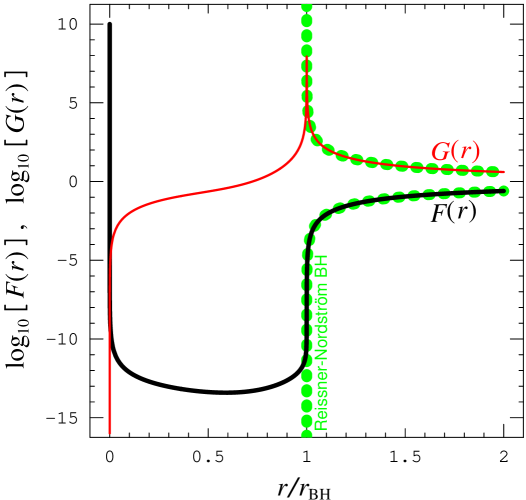
Figure 2: Elements of the metric $F(r)$ and $G(r)$ in the solution. The thick solid (black) curve is $F(r)$ and the thin solid (red) curve is $G(r)$. The thick dotted (green) curves indicate the exterior part ($r>r_{\rm BH}$) of the Reissner-Nordström metric ($F_{\rm BH}(r)$ and $G_{\rm BH}(r)$ in (21)) with the same radius $r_{\rm BH}$ and with the same charge $q$.

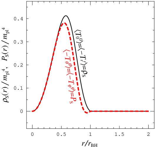
Figure 3: Distribution of the expectation values of the energy momentum tensor for the quantized scalar field $\left<{\rm 1s}\left|T_{{\rm S}\mu}^{\ \ \nu}\right|{\rm 1s}\right>$. The thin solid (black) curve is $\rho_{\rm S}=\left<T_{0}^{\ 0}\right>=-\left<T_{r}^{\ r}\right>$. The thick dotted (red) curve is $P_{\rm S}=\left<T_{\theta}^{\ \theta}\right>=-\left<T_{\varphi}^{\ \varphi}\right>$. $\rho_{\rm S}$ is positive definite but $P_{\rm S}$ becomes negative at $r\simeq r_{\rm BH}$.

According to the solution, the quantum fluctuation of the scalar field is localized in the ball whose radius corresponds with the Schwarzschild radius (see Figure 1). Also the energy-density and the pressures of the scalar field are localized in the ball (see Figure 3). The shapes of the metric-elements in our solution are qualitatively equivalent to those in the radiation-ball solution for charged black holes [9]. The form of the metric element $F(r)$ shows that there is a gravitational potential-well in the ball. Therefore the quantum fluctuation is binded into the ball by the gravitation and the gravitation is made by the singularity, the electromagnetic field and the quantum fluctuation. Everything in the exterior of the ball corresponds with the charged black hole with the same charge $q$ except for the region extremely near the ball. We conclude that the solution realizes our proposal presented in the first section.

When we change the charge parameter ($q=0.99999,0.9999,0.999$) within the range which can be regarded as near-extremal or when we change the red-shift parameter ($\alpha=1,10,100$), there is almost no change in the radius of the solution $r_{\rm BH}$, the radial mode-function $\tilde{f}(r)$ and the expectation value of the energy-momentum tensor $\left<{\rm 1s}\left|T_{{\rm S}\mu}^{\ \ \nu}(r)\right|{\rm 1s}\right>$. When $\alpha$ becomes much larger or when $q$ becomes much smaller, the border of the ball becomes fuzzy. When $q$ approaches to 1 (extremal charge) or when $\alpha$ becomes small, the potential-well ($F(r)$ in the ball) becomes deep with keeping both $\tilde{f}(r)$ and $\left<{\rm 1s}\left|T_{{\rm S}\mu}^{\ \ \nu}(r)\right|{\rm 1s}\right>$. When the potential-well becomes deep, the frequency $\omega_{1}$ becomes small according to the dependency in (54).

4 Conclusion and Discussion

We proposed a concept for the structure model of the black holes by the mean field approximation. The structure of the black hole, which consists of both a central singularity and a ball of the quantum-fluctuation of the fields, is similar to the atomic structure. Especially we concretely constructed the minimal structure model for near extremal-charged black hole. The minimal structure model contains a single quantum of the field-fluctuation. The structure of the minimal model is quite similar to that of the hydrogen atom and has the minimal Schwarzschild radius $r_{\rm BH}=1.12871\times l_{\rm pl}$.

While our model describes the near extremal-charged black hole, we expect that the model also describes the extremal limit $(q\rightarrow 1)$. The situation of our model is the same as that of the radiation ball model for charged black hole [9] where the extremal-charged black hole was expected to be described as “the fully frozen radiation-ball”. Our model of the extremal limit has the same $\tilde{f}(r)$ in Figure 1 and the same $\left<{\rm 1s}\left|T_{{\rm S}\mu}^{\ \ \nu}(r)\right|{\rm 1s}\right>$ in Figure 3. The distribution of the metric element $G(r)$ in the extremal limit corresponds with that in the non-extremal solution except for the divergence of $G(r)$ on the peak at $r=r_{\rm BH}$ (see Figure 2). For the extremal limit, the potential-well becomes infinitely deep and the quantum-fluctuation freezes up because the metric element $F(r)$ in the ball goes to zero and the frequency $\omega_{1}$ also goes to zero. The exterior region $(r>r_{\rm BH})$ of our solution with the extremal limit fully corresponds with that of the extremal-charged black hole.

The concrete construction of the non-minimal model which contains multiple quanta is important subject. This subject is technically complicated because we should solve simultaneous equations including unknown functions of the same number as the quanta. When we find the solution, we can compare the entropy of the model and that of the black hole. The subject is related with analyzing the process of the Hawking radiation in the model of the black hole whose charge is much smaller than the extremal-charge.

The minimal model cannot determine the red-shift parameter $\alpha$ of the singularity by itself. The radiation ball model can determine the parameter $\alpha$ as $1$ because the model derives the Hawking radiation as thermal equilibrium [8, 9]. Therefore analyzing the Hawking radiation from the ball determines the parameter.

We adopted the approximation of representing all of the field-fluctuations by $g_{\rm dof}$ kinds of the real scalar fields. According to our mean field approximation of the gravity, only the interaction with the mean-field gravity is important. Then the approximation of the scalar fields is justified. The result similar to ours is expected by more proper analysis of graviton, photon, fermion and so on.

The minimal structure model has the entropy $\log g_{\rm dof}$ because the quantum in the ball belongs to one of $g_{\rm dof}$ kinds of fields. If we assume that the Bekenstein’s entropy $S=(1/4)4\pi r_{\rm BH}^{2}$ in [1] is always correct, the entropy of the ball becomes about $4$ and the degree of freedom $g_{\rm dof}=\exp S$ becomes about $54$. While twice of $g_{\rm dof}$ is similar to the degree of freedom in the Standard Model, the meaning of this is not clear.

ACKNOWLEDGMENTS

I would like to thank Ofer Aharony, Micha Berkooz, Hiroshi Ezawa, Satoshi Iso, Barak Kol, Masao Ninomiya and Kunio Yasue for useful discussions. I am grateful to Kei Shigetomi for helpful advice and also for careful reading of the manuscript. The work has been supported by the Okayama Prefecture.

Appendix

As an example we present the full expression of a element of the energy-momentum tensor as

$$T_{0}^{\ 0} = \sum_{n_{1}m_{1}l_{1}}\sum_{n_{2}m_{2}l_{2}}\frac{1}{\sqrt{2\omega_{n_{1}}C_{n_{1}l_{1}}}}\frac{1}{\sqrt{2\omega_{n_{2}}C_{n_{2}l_{2}}}}$$ (56)

$$\qquad\;\times\;\frac{1}{2}\Biggl{[}\;+\;\omega_{n_{1}}\omega_{n_{2}}\frac{1}{F}f_{n_{1}l_{1}}f_{n_{2}l_{2}}Y_{l_{1}}^{\ m_{1}}Y_{l_{2}}^{\ m_{2}}\;+\;\frac{1}{G}\partial_{r}f_{n_{1}l_{1}}\partial_{r}f_{n_{2}l_{2}}Y_{l_{1}}^{\ m_{1}}Y_{l_{2}}^{\ m_{2}}$$

$$\qquad\qquad\ \ \;+\;\frac{1}{r^{2}}f_{n_{1}l_{1}}f_{n_{2}l_{2}}\left(\partial_{\theta}Y_{l_{1}}^{\ m_{1}}\partial_{\theta}Y_{l_{2}}^{\ m_{2}}+\frac{\partial_{\varphi}Y_{l_{1}}^{\ m_{1}}\partial_{\varphi}Y_{l_{2}}^{\ m_{2}}}{\sin^{2}\theta}\right)\Biggr{]}$$

$$\qquad\;\times\;\left(e^{-i(\omega_{n_{1}}-\omega_{n_{2}})t}a_{n_{1}m_{1}l_{1}}a_{n_{2}m_{2}l_{2}}^{\dagger}+e^{+i(\omega_{n_{1}}-\omega_{n_{2}})t}a_{n_{1}m_{1}l_{1}}^{\dagger}a_{n_{2}m_{2}l_{2}}\right)$$

$$+ \sum_{n_{1}m_{1}l_{1}}\sum_{n_{2}m_{2}l_{2}}\frac{1}{\sqrt{2\omega_{n_{1}}C_{n_{1}l_{1}}}}\frac{1}{\sqrt{2\omega_{n_{2}}C_{n_{2}l_{2}}}}$$

$$\qquad\;\times\;\frac{1}{2}\Biggl{[}\;-\;\omega_{n_{1}}\omega_{n_{2}}\frac{1}{F}f_{n_{1}l_{1}}f_{n_{2}l_{2}}Y_{l_{1}}^{\ m_{1}}Y_{l_{2}}^{\ m_{2}}\;+\;\frac{1}{G}\partial_{r}f_{n_{1}l_{1}}\partial_{r}f_{n_{2}l_{2}}Y_{l_{1}}^{\ m_{1}}Y_{l_{2}}^{\ m_{2}}$$

$$\qquad\qquad\ \ \;+\;\frac{1}{r^{2}}f_{n_{1}l_{1}}f_{n_{2}l_{2}}\left(\partial_{\theta}Y_{l_{1}}^{\ m_{1}}\partial_{\theta}Y_{l_{2}}^{\ m_{2}}+\frac{\partial_{\varphi}Y_{l_{1}}^{\ m_{1}}\partial_{\varphi}Y_{l_{2}}^{\ m_{2}}}{\sin^{2}\theta}\right)\Biggr{]}$$

$$\qquad\;\times\;\left(e^{-i(\omega_{n_{1}}+\omega_{n_{2}})t}a_{n_{1}m_{1}l_{1}}a_{n_{2}m_{2}l_{2}}+e^{+i(\omega_{n_{1}}+\omega_{n_{2}})t}a_{n_{1}m_{1}l_{1}}^{\dagger}a_{n_{2}m_{2}l_{2}}^{\dagger}\right).$$

Only the first half of the expression (56) contributes to the expectation value of the eigenstate for the Hamiltonian.

References

• [1] J.ย D.ย Bekenstein, Phys.ย Rev.ย D 7, 2333 (1973).
• [2] S.ย W.ย Hawking, Commun.ย Math.ย Phys.ย  43, 199 (1975).
• [3] S.ย W.ย Hawking, Nature 248, 30 (1974).
• [4] A.ย Strominger and C.ย Vafa, Phys.ย Lett.ย B 379, 99 (1996) [arXiv:hep-th/9601029].
• [5] G.ย T.ย Horowitz and A.ย Strominger, Phys.ย Rev.ย Lett.ย  77, 2368 (1996) [arXiv:hep-th/9602051].
• [6] K.ย Hotta, Prog.ย Theor.ย Phys.ย  99, 427 (1998) [arXiv:hep-th/9705100].
• [7] N.ย Iizuka, D.ย Kabat, G.ย Lifschytz and D.ย A.ย Lowe, arXiv:hep-th/0306209.
• [8] Y.ย Nagatani, arXiv:hep-th/0310185.
• [9] Y.ย Nagatani, arXiv:hep-th/0311133.
• [10] Y.ย Nagatani, arXiv:hep-th/0312060.
• [11] Y.ย Nagatani, arXiv:hep-th/0307295.