Abstract

We study the Type 0A string theory in the $(2,4k)$ superconformal minimal model backgrounds, focusing on the fully non–perturbative string equations which define the partition function of the model. The equations admit a parameter, $\Gamma$, which in the spacetime interpretation controls the number of background D–branes, or R–R flux units, depending upon which weak coupling regime is taken. We study the properties of the string equations (often focusing on the $(2,4)$ model in particular) and their physical solutions. The solutions are the potential for an associated Schrödinger problem whose wavefunction is that of an extended D–brane probe. We perform a numerical study of the spectrum of this system for varying $\Gamma$ and establish that when $\Gamma$ is a positive integer the equations’ solutions have special properties consistent with the spacetime interpretation. We also show that a natural solution–generating transformation (that changes $\Gamma$ by an integer) is the Bäcklund transformation of the KdV hierarchy specialized to (scale invariant) solitons at zero velocity. Our results suggest that the localized D–branes of the minimal string theories are directly related to the solitons of the KdV hierarchy. Further, we observe an interesting transition when $\Gamma=-1$.

1 Background

The $(2,4k)$ series of the minimal type 0A string theory, in the presence of background R–R sources, has a non–perturbative definition via the following “string equation”[1]:

$$u{\cal R}^{2}-\frac{1}{2}{\cal R}{\cal R}^{{}^{\prime\prime}}+\frac{1}{4}({\cal R}^{{}^{\prime}})^{2}=\nu^{2}\Gamma^{2}\ .$$ (1)

Here $u(z)$ is a real function of the real variable $z$; a prime denotes $\nu\partial/\partial z$; and $\Gamma$ and $\nu$ are constants. The quantity $\mathcal{R}$ is defined by:

$${\cal R}=\sum_{k=0}^{\infty}\left(k+\frac{1}{2}\right)t_{k}R_{k}\ ,$$ (2)

where the $R_{k}$ ($k=0,\ldots$) are polynomials in $u(z)$ and its $z$–derivatives. They are related by a recursion relation:

$$R^{{}^{\prime}}_{k+1}=\frac{1}{4}R^{{}^{\prime\prime\prime}}_{k}-uR^{{}^{\prime}}_{k}-\frac{1}{2}u^{\prime}R_{k}\ ,$$ (3)

and are fixed by the constant $R_{0}$, and the requirement that the rest vanish for vanishing $u$. The first few are:

$$R_{0}=\frac{1}{2}\ ;\quad R_{1}=-\frac{1}{4}u\ ;\quad R_{2}=\frac{1}{16}(3u^{2}-u^{{}^{\prime\prime}})\ .$$ (4)

The $k$th model is chosen by setting all the other $t\,$s to zero except $t_{0}\equiv z$, and $t_{k}$, the latter being fixed to a numerical value such that ${\cal R}={\cal D}_{k}-z$. The ${\cal D}_{k}$ are normalised such that the coefficient of $u^{k}$ is unity, e.g.:

$${\cal D}_{1}=u\ ,\quad{\cal D}_{2}=u^{2}-\frac{1}{3}u^{{}^{\prime\prime}}\ ,\quad{\cal D}_{3}=u^{3}-uu^{{}^{\prime\prime}}-\frac{1}{2}(u^{{}^{\prime}})^{2}+\frac{1}{10}u^{{}^{\prime\prime\prime\prime}}\ .$$ (5)

For the $k$th model, equation (1) has asymptotics:

$$u(z) = z^{\frac{1}{k}}+\frac{\nu\Gamma}{kz^{1-\frac{1}{2k}}}+\cdots\quad\mbox{\rm for}\quad z\longrightarrow+\infty\ ,$$

$$u(z) = \frac{\nu^{2}(4\Gamma^{2}-1)}{4z^{2}}+\cdots\quad\mbox{\rm for}\quad z\longrightarrow-\infty\ .$$ (6)

The function $u(z)$ defines the partition function $Z=\exp(-F)$ of the string theory via:

$$u(z)=\nu^{2}\frac{\partial^{2}F}{\partial\mu^{2}}\Biggl{|}_{\mu=z}\ ,$$ (7)

where $\mu$ is the coefficient of the lowest dimension operator in the world–sheet theory. Integrating twice, the asymptotic expansions in equations (6) furnish the partition function perturbatively as an expansion in the dimensionless string coupling

$$g_{s}={\nu\over\mu^{1+{1\over 2k}}}\ .$$ (8)

The role of $\Gamma$ is now clear: at large positive $z$ we find that $\Gamma$ controls the number of background D-branes since the perturbative series contains both open and closed string worldsheets with a factor of $\Gamma$ for each boundary; while the large negative $z$ series gives only closed string worldsheets, with $\Gamma^{2}$ appearing when there is an insertion of pure R–R flux[1, 2].

From the point of view of the $k$th theory, the other $t_{k}$s represent coupling to closed string operators ${\cal O}_{k}$. It is well known that the insertion of each operator can be expressed in terms of the KdV flows[3, 4]:

$$\frac{\partial u}{\partial t_{k}}=R^{{}^{\prime}}_{k+1}\ .$$ (9)

The operator ${\cal O}_{0}$ couples to $t_{0}$, which is in fact $-4z$, the cosmological constant (in the unitary model). So ${\cal O}_{0}$ is often referred to as the puncture operator, which yields the area of a surface by fixing a point which is then integrated over in the path integral. So $u(z)$ is the two–point function of the puncture operator.

For $\Gamma=0$ the string equation (1) was discovered by defining a family of string theories using double scaled models of a complex matrix $M$:

$${\cal Z}=\int dM\exp\left\{-\frac{N}{\gamma}{\rm{\rm Tr}}\left(V(MM^{\dagger})\right)\right\}\ .$$ (10)

The resulting physics captured by the string equation was the first complete non–perturbative definition of a string theory[5, 6, 7, 8, 9], sharing the large $z$ perturbation theory of the original (bosonic) string theories obtained by double scaling of Hermitian matrix models[10, 11, 12], but not suffering from their non–perturbative shortcomings.

Non–zero $\Gamma$ can also be studied using a matrix model definition in a variety of ways. One way is to add a logarithmic term[13, 14] to an appropriate[1, 15] matrix model potential. Expanding the logarithm clearly adds holes of all sizes to the string worldsheets defined by studying the duals of the Feynman diagrams of the model. Another (equivalent) method is to define $M$ as an $(N+\Gamma)\times N$ rectangular matrix[16, 2]. The double scaling limit (in which $N$ is taken large) then yields equation (1).

It is clear from these two methods that, in the interpretation of the matrix model as the world–volume theory of $N$ D–branes (which defines the closed string theory holographically[17] after taking the double scaling limit), the modification corresponds to adding $\Gamma$ “quark flavours” to the world–volume model. This corresponds to adding sectors of open strings stretching between the $N$ D–branes and $\Gamma$ extra D–branes.

So from this point of view it appears that $\Gamma$ is a positive integer. However, this is not at all clear from the string equation itself. In fact, it is known perturbatively that the solutions of the equation have special properties for various fractional values of $\Gamma$ . These might well turn out to be unphysical values, but this is not à priori clear. One of the purposes of this paper is to show that $\Gamma$ being a positive integer is in fact selected out as special from the point of view of the string equation. We will do this by studying the equation non–perturbatively using numerical methods, and by also observing the properties of a natural transformation between solutions of the string equation which change $\Gamma$ by $\pm 1$. This transformation was discovered in ref[1], and we derive an explicit form for it here, and employ this form in our investigations. We further observe that the transformation is in fact a specialisation (to the scale invariant soliton sector) of the Bäcklund transformations of the KdV hierarchy!

These Bäcklund transformations are known to change the soliton number of solutions of the KdV equation (and its higher order analogues)[18], and so our observation is particularly intriguing, since it implies that the (localized[19]) D–branes of the minimal type 0A string theory are intimately connected with the solitons of the KdV hierarchy.

Note: While this paper was being written, a paper appeared[20] which contains results that have some overlap with ours.

2 A Spectral Problem

A solution $u(z)$ of the string equation serves as the potential for a one–dimensional Hamiltonian ${\cal H}$ which arises naturally in the double–scaled matrix model[21]:

$${\cal H}=-Q=-\nu^{2}\frac{\partial^{2}}{\partial z^{2}}+u(z)\ ,$$ (11)

where $\sqrt{2}\,\nu$ plays the role of $\hbar$.

In fact, the (first derivative of) the string equation can be obtained by eliminating the wave–function $\psi(z)$ from the equations:

$$Q\psi = \lambda_{s}\psi\ ,$$

$${\widetilde{P}}\psi = \lambda_{s}{\partial\over\partial\lambda_{s}}\psi\ .$$ (12)

Here, ${\widetilde{P}}$ is a differential operator representing scale transformations. It is constructed from (the differential operator part of) fractional powers[22, 23] of $Q$, as follows[6]:

$${\widetilde{P}}=\sum_{k=1}^{\infty}\left(k+\frac{1}{2}\right)t_{k}Q_{+}^{k+\frac{1}{2}}-\frac{1}{2}z\frac{\partial}{\partial z}+{\rm const.}\ .$$ (13)

Eliminating $\psi$, one has the operator equation[6]:

$$[{\widetilde{P}},Q]=Q\ ,$$ (14)

which yields an equation for $u(z)$ which is the first derivative of equation (1).

The spectrum of this model has interesting and important information, and is a rather direct way of getting access to the non–perturbative physics of the model.  The problem is naturally defined in terms of the eigenvalues, $\lambda$, of the combination $MM^{\dagger}$. These are naturally positive. So in the double scaling limit (which focuses on the infinitesimal region near the tail of the eigenvalue distribution of the model) the scaled eigenvalues, which we denote as $\lambda_{s}$, are also distributed on the positive real line.

We verified this in the full non–perturbative regime by studying the spectrum of ${\cal H}$ numerically. To do this we solved the differential equation for a given value of $k$ as a boundary value problem, with the perturbative boundary conditions given in equations (6). We started out by using the equation–solving routine dsolve in the package Maple 9, although later we used other methods (see below for the case of negative $\Gamma$). We used a discrete $z$ lattice of up to $8192$ points for positive $\Gamma$.

First, note the form of the function $u(z)$ for some strictly positive values of $\Gamma$ (see figure 1).

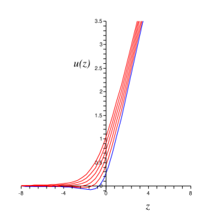
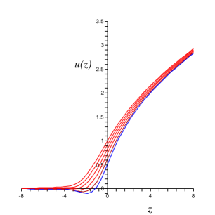
Figure 1: Numerical solutions to equation (1) for $u(z)$: (a) The case $k=1$, and (b) the case $k=2$, for a range of values of the parameter $\Gamma$. The very bottom curve in each case has $\Gamma=0$. The solutions all asymptote to $u=z^{1/k}$ for large positive $z$ and $u=0$ for large negative $z$.

Since the potential tends to zero at $z\to-\infty$, and rises monotonically in the $z\to+\infty$ limit, it is clear that the spectrum has the chance to be both continuous and bounded from below by zero, as we expect from perturbation theory. A striking feature is the fact that the potential develops a potential well in the interior, as $\Gamma\to 0$.

It is therefore interesting and important to non–perturbatively establish these properties (continuity, boundedness) of the spectrum for various $\Gamma$. First, we checked the spectrum of the case $\Gamma=0$ (the case with no background branes), and verified that there are no bound states, despite the appearance of the well. We set up the problem numerically by discretizing the spatial coordinate $z$, typically using the interval $-10\leq z\leq+10$, with $\nu=1$. We used a range of lattice spacings in studying our problem to ensure stability. This was equivalent to a number of lattice points ranging from as little as 500 up to 10000 (the latter used when more accuracy was needed, as we shall see later on.) Discretizing this problem turns it into a problem of diagonalizing a tri–diagonal matrix for which we coded a fairly efficient well–known method (the TQLI method[26]) in C$++$ to do the work. This allowed us to establish non–perturbatively with some confidence that there are no bound states in the well for positive $\Gamma$, and so the spectrum is continuous and bounded from below by zero, in accord with perturbative expectations.

The next step is the case of negative $\Gamma$, which is clearly allowed by the equation and so should be studied. Our first observation is that solving the differential equation numerically became much more prone to error, and we had to use much more accurate methods. We used the NAG library of routines for solving boundary value problems with C$++$ to make further progress, as they gave much greater control over the problem. We were able to construct directly in this way a solution for $u(z)$ for values as low as $\Gamma=-0.970$ before running into numerical problems. See figure 2.

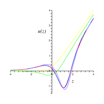
Figure 2: Numerical solutions to equation (1) for $u(z)$ in the case $k=1$, for a range of negative values of the parameter $\Gamma$: $0.000,-0.500,-0.950,-0.965,-0.968,-0.970$.

Once again we should check that the perturbative expectation that the spectrum is positive persists non–perturbatively. Several solutions $u(z)$, for various $\Gamma$ down to $-0.970$ were used as potentials for ${\cal H}$ and found (upon placing in our tridiagonal matrix diagonalization routine) to have no bound states.

With these methods, the growing instability is suggestive, but not compellingly so, that something interesting might be happening at $\Gamma=-1$. In order to establish this more satisfyingly we employed some exact methods (in the form of a solution–generating transformation), which we will describe next. This will allow us to generate new $u(z)$ from the ones we already can extract numerically, and allow us to approach $\Gamma=-1$ in a controlled manner, and with convincing accuracy.

3 Bäcklund Transformations

In ref.[1], it was established that the double scaled unitary matrix models of refs.[27, 28] had an interpretation as continuum string theories with open string sectors. This was done by establishing a direct connection between the solutions of the string equations in equation (1) and solutions of the string equations for those unitary matrix models, which are most naturally written in terms of the quantities $S_{k}$, where:

$$S_{k}\equiv\frac{1}{2}R_{k}^{\prime}[v^{2}+v^{\prime}]-vR_{k}[v^{2}+v^{\prime}]\ ,$$ (15)

as:

$$\sum_{k=1}^{\infty}\left(k+\frac{1}{2}\right)t_{k}S_{k}[v(z)]+zv(z)=\nu C\ .$$ (16)

The models are organised by the mKdV hierarchy:

$$\frac{\partial v}{\partial t_{k}}=\frac{1}{2}S^{\prime}_{k}[v]\ .$$ (17)

We define $u(z)$ and $v(z)$ such that:

$$X_{\pm}[u,v]\equiv\frac{1}{2}\mathcal{R}^{\prime}[u]\mp\nu\Gamma-v(z)\mathcal{R}[u]=0\ ,$$ (18)

which implies a specific form for $v(z)$ given a $u(z)$:

$$v=\frac{\frac{1}{2}\mathcal{R}^{\prime}[u]\mp\nu\Gamma}{\mathcal{R}[u]}\ .$$ (19)

Noting the identity[1]:

$$0=X_{\pm}^{2}\pm\nu\Gamma X_{\pm}-\mathcal{R}[u]X_{\pm}^{\prime}\equiv(v^{2}+v^{\prime})\mathcal{R}^{2}[u]-\frac{1}{2}\mathcal{R}[u]\mathcal{R}^{\prime\prime}[u]+\frac{1}{4}(\mathcal{R}^{\prime}[u])^{2}-\nu^{2}\Gamma^{2}\ ,$$ (20)

we see that if the inverse transformation $u=v^{2}+v^{\prime}$ (known in the integrable literature as the Miura map) exists, then this is just our original string equation (1); and on substitution into equation (19) gives equation (16) with $C=1/2\pm\Gamma$. Since the unitary matrix models of refs.[27, 28] were originally derived with $C=0$, those models turn out to be identified with the case $\Gamma=1/2$.

Since the transformation is true for both values of $C$ we find that a given $u(z)$ for a value of $\Gamma$ gives two functions $v_{C}(z)$ and $v_{1-C}(z)$, which must be related by:

$$v_{C}^{2}+v_{C}^{\prime}=v_{1-C}^{2}+v_{1-C}^{\prime}\ ,$$ (21)

and hence:

$$v_{1-C}=v_{C}+\frac{2C-1}{\mathcal{R}[v_{C}^{2}+v_{C}^{\prime}]}\ .$$ (22)

On the other hand, the string equation (16) has the symmetry $v_{-C}=-v_{C}$, and so we obtain a result which relates $v(z)$ at one value of $C$ to another for $C\pm 1$:

$$v_{C\pm 1}=-v_{C}-\frac{2C\pm 1}{\mathcal{R}[v_{C}^{2}\mp v_{C}^{\prime}]}\ .$$ (23)

This implies a similar transformation for functions $u(z)$, relating $\Gamma$ and $\Gamma\pm 1$. We can make this explicit by combining equations (19), (20), (23) and $u=v^{2}+v^{\prime}$ to give the remarkable result:

$$u_{\Gamma\pm 1}=\frac{3\left(\mathcal{R}^{\prime}\right)^{2}-2\mathcal{R}\mathcal{R}^{\prime\prime}\mp 8\nu\Gamma\,\mathcal{R}^{\prime}+4\nu^{2}\Gamma^{2}}{4\mathcal{R}^{2}}\ ,$$ (24)

where $\mathcal{R}\equiv\mathcal{R}(u_{\Gamma})$.

In the theory of non–linear differential equations (such as those encountered in the integrable model context) Bäcklund transformations are extremely useful, since they convert a given solution of the differential equation into a new solution. Strictly speaking, it looks rather like this is not what we have here since our string equation (1) is displayed with $\Gamma$ explicitly appearing, so $u_{\Gamma}$ and $u_{\Gamma\pm 1}$ are solutions of different equations. However, the once–differentiated string equation (which is in fact the one which appears naturally in many derivations; see the beginning of the previous section, and see below), which is

$$\frac{1}{2}{\cal R}^{\prime\prime\prime}-2u{\cal R}^{\prime}-u^{\prime}{\cal R}=0\ ,$$ (25)

does not have an explicit appearance of $\Gamma$. The solutions $u_{\Gamma}$ do know of $\Gamma$, of course, since it appears (for example) in their asymptotic expansion (6).

So we have a genuine Bäcklund transformation for our system. What is particularly interesting is that it is not just any such transformation but a special case of the well–known Bäcklund transformations known to change the number of solitons in the KdV hierarchy. We can make this explicit as follows:

We start with the KdV equations (9), which we rewrite as:

$$\frac{\partial{\tilde{u}}}{\partial t_{k}}=R^{\prime}_{k+1}[{\tilde{u}}]=\left(\frac{1}{4}\mathrm{d}^{3}-{\tilde{u}}\mathrm{d}-\frac{1}{2}\frac{\partial{\tilde{u}}}{\partial x}\right)R_{k}[{\tilde{u}}]\ ,$$ (26)

where now $d\equiv\frac{\partial}{\partial x}$.

We can search for solutions of the form ${\tilde{u}}(x,t_{k})=t_{k}^{2\beta_{k}}u(xt_{k}^{\beta_{k}})$. We then find $\beta_{k}=-1/(2k+1)$ and that (under appropriate rescaling of $t_{k}$) equation (26) becomes:

$$-u-\frac{1}{2}zu^{\prime}=\left(\frac{1}{4}\mathrm{d}^{3}-u\mathrm{d}-\frac{1}{2}u^{\prime}\right)R_{k}[u]\ ,$$ (27)

where a prime denotes differentiation with respect to $z=xt^{\beta_{k}}$. Re–arranging we find the once–differentiated string equation (25) for a particular $k$.

This is another way of making the observation (already noted in ref.[6]) that the string equation follows a restriction of the KdV hierarchy to scale invariant solutions. This also fits with the recovery[6] of the string equation from the operator relation $[{\widetilde{P}},Q]=Q$, where ${\widetilde{P}}$ is the generator of scale transformations. (See the previous section.)

Now note that the KdV hierarchy admits the following well known Bäcklund transformation relating a solution ${\tilde{u}}_{1}$ to a solution ${\tilde{u}}_{2}$:

$$w_{x}+y_{x}=\frac{1}{2}(w-y)^{2}+2{\tilde{\lambda}}\ ,$$ (28)

where $w_{x}={\tilde{u}}_{1}$ and $y_{x}={\tilde{u}}_{2}$.

This can be derived from the (generalised) Miura map ${\tilde{u}}=v^{2}+v^{\prime}+{\tilde{\lambda}}$ (where ${\tilde{\lambda}}$ is a constant), which relates the KdV and mKdV hierarchies, by noting that the mKdV flow hierarchy (see equation (17)) is invariant under $v\rightarrow-v$. So we can have two solutions of KdV, ${\tilde{u}}_{1}$ and ${\tilde{u}}_{2}$, arising from the same solution, $v$, of the mKdV hierarchy.

We have ${\tilde{u}}_{1}=w_{x}=v^{2}+v^{\prime}+{\tilde{\lambda}}$ and ${\tilde{u}}_{2}=y_{x}=v^{2}-v^{\prime}+{\tilde{\lambda}}$, which gives upon addition and subtraction:

$$w_{x}+y_{x}=2v^{2}+2{\tilde{\lambda}}\ ,\quad w_{x}-y_{x}=2v^{\prime}\ .$$ (29)

The latter can then be integrated once and substituted into the former to give equation (28). This can then be specialized to solutions of the string equation by writing ${\tilde{u}}_{i}=t^{2\beta_{k}}u_{i}(xt^{\beta_{k}})\equiv t^{2\beta_{k}}f_{i}^{\prime}(xt^{\beta_{k}})$, which gives:

$$w=t^{\beta_{k}}f_{1}(xt^{\beta_{k}})\ ,\qquad y=t^{\beta_{k}}f_{2}(xt^{\beta_{k}})\ ,$$ (30)

where a prime denotes differentiation with respect to $z=xt^{\beta_{k}}$. We have therefore

$$f_{1}^{\prime}+f_{2}^{\prime}=\frac{1}{2}(f_{1}-f_{2})^{2}+2{\tilde{\lambda}}t^{-2\beta_{k}}\ .$$ (31)

So we see that for consistency we must set ${\tilde{\lambda}}=0$, which has an interesting interpretation to be discussed below. Hence we have

$$f_{1}^{\prime}+f_{2}^{\prime}=\frac{1}{2}(f_{1}-f_{2})^{2}\ .$$ (32)

So far, it is not clear that this transformation changes $\Gamma$. In order to establish the connection between this transformation and the one displayed in equation (24), in which $\Gamma$ appears explicitly, we first work perturbatively. Starting with the asymptotic expansions (6), for (say) $u_{1}$, it is easy to show that using equation (32) the asymptotic expansion obtained for $u_{2}$ is of the same form, except that $\Gamma$ has been replaced by $\Gamma\pm 1$. We then expect that they are equivalent non–perturbatively, and have checked that this is the case by working numerically on some explicit solutions.

So we have established that the Bäcklund transformation takes us between solutions with asymptotics given in equation (6) which are for $\Gamma$s differing from each other by unity. It is known[18] that the Bäcklund transformations (28) of KdV increase or decrease the soliton number of a given solution by unity. In fact, for a given solution $u$, the soliton corresponds to a bound state of ${\cal H}$ with (negative) eigenvalue ${\tilde{\lambda}}$, and the speed of the soliton is given by $-{\tilde{\lambda}}$ (up to a positive numerical constant). The soliton number of a particular solution can be read off by the number of such bound states and their individual velocities are set by the discrete spectrum.

In our case, we have established (so far) that there are no bound states in our solutions, and indeed, our restriction of the Bäcklund transformation forces ${\tilde{\lambda}}=0$. So we deduce from this that $\Gamma$, which counts soliton number, must count the number of zero–velocity solitons. This is another sign that $\Gamma$ is naturally integer, and positive. We will shortly find further evidence for this.

Now that we have a method for generating new solutions $u(z)$ starting from old ones, we can return to our numerical study armed with more powerful tools.

4 The Case of $\Gamma=-1$

We established in the last section that given a solution $u_{\Gamma}$, we can generate a solution $u_{\Gamma\pm 1}$. In the section before, we reported that it was difficult to solve the string equation numerically as $\Gamma$ became more negative. Numerical precision was lost rapidly as $\Gamma$ went below the value $-0.9$, while positive $\Gamma$ is very much under control. We can use our transformation from the previous section to surmount this obstacle, by simply solving the equation numerically for $u(z)$ for $\Gamma=\epsilon$, for $\epsilon$ small and positive, and then use our transformation (24) to build a solution for $u(z)$ with $\Gamma=-1+\epsilon$. We can simply follow $\epsilon$ to vanishingly small values and therefore learn the properties of $u(z)$ on the approach to $\Gamma=-1$.

We carried this out with very interesting results. See figure 3 for examples. We were able to use this method to generate $u(z)$ for $\Gamma=-1+\epsilon$ where $\epsilon$ could easily be taken as small as $\sim 10^{-10}$. The potential well is observed to get more deep and narrow increasingly rapidly as $\epsilon\to 0$. In fact, we observe numerically that the well runs to infinity along the line $u(z)=-z$, becoming infinitely deep and narrow in the limit $\Gamma=-1$.

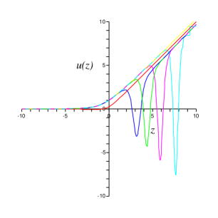
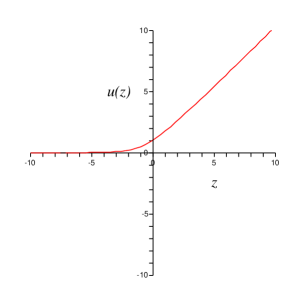
Figure 3: Numerical solutions to equation (1) for $u(z)$ in the case $k=1$. The set of curves on the left shows $u(z)$ for a range of negative values of the parameter $\Gamma$, closely approaching the value $-1$ from above. The curve with the lowest well (very close to $\Gamma=-1$) is beginning to show signs of numerical error to the right. The curve on the right is the case of $\Gamma=+1$, used for comparison in the text.

Most interestingly, note that since the deepening of the well is accompanied by a narrowing, the system has a chance of preventing the appearance of a dangerous bound state. We used the families of $u(z)$ functions found here as potentials for ${\cal H}$ and were indeed able to verify with some confidence (to within acceptable error tolerance) that there were no bound states present for any of the potentials.

So the case $\Gamma=-1$ is remarkably special, and in fact contains a surprise. At first, it seems that it develops a pathology, since as $\epsilon\to 0$ the well was seen to grow infinitely deep, but at the same time it became extremely narrow and, moreover, it moved off to infinity to the right. So the solution may in fact be well–behaved. In support of this, it is interesting to note the striking fact (again, from studying families of curves such as those displayed in figure 3) that in the limit the $\Gamma=-1$ curve looks rather like the $\Gamma=+1$ curve! The feature associated to the well is confined to a highly localized narrow (and deep) region, which has moved away. Everything that remains of the $\Gamma=-1$ curve at finite $z$ falls (with considerable numerical accuracy) on the $\Gamma=+1$ curve.

This numerical observation suggests the surprising result that the functions $u_{\Gamma=-1}$ and $u_{\Gamma=+1}$ are actually identical, and that the discrepancy from the piece at infinity actually disappears in the limit. We can prove this for all $k$. The transformation (24) can be used to generate either of these functions starting with the case of $u_{\Gamma=0}$. Putting this function and $\Gamma=0$ into the equation immediately gives the result that $u_{\Gamma=-1}=u_{\Gamma=+1}$, since there is no explicit appearance of $\Gamma$ in the transformation in order to generate the difference between decreasing vs increasing $\Gamma$.

Note that below $\Gamma=-1$ there is a transition to completely new behaviour. There, the system no longer has a smooth solution with the asymptotics given in equation (6), and there must be a singularity at finite $z$. The origin of the singularity can be seen (for $k=1)$ by considering the form of the transformation (24). The denominator of the transformation is $4\mathcal{R}^{2}$, where, for large positive $z$, we have that

$${\cal R}=u^{k}-z\simeq\frac{\nu\Gamma}{z^{\frac{1}{2k}}}+\cdots\ ,$$ (33)

and so for $\Gamma<0$, the $k=1$ solution must approach the line $u=z$ from below as $z\to+\infty$. Since $u(z)$ started out above this line (at $z\to-\infty$), it must be that it crosses the line somewhere in the interior. If this is the case, then somewhere in the interior, the new solution $u_{\Gamma-1}$ must have a singularity, since the denominator vanishes there. We expect similar arguments to hold for the negative $\Gamma$ behaviour of other values of $k$.

So we have the very natural physical situation singling out $\Gamma$ as a positive integer, since any solution $u(z)$ with $-1<\Gamma<0$ can be used as a seed for our transformation (24) to generate a $u(z)$ solution with poles, which have a problematic interpretation. Furthermore, any solution $u(z)$ for a positive fractional value of $\Gamma$ can also be used, by applying the transformation successively, to generate such solutions, and so they are in the same class as the $-1<\Gamma<0$ solutions. The $u(z)$ for positive integer values of $\Gamma$ are therefore special, in that they are not connected by our transformation to any solutions with poles.

5 Summary

So we see that studying the string equation non–perturbatively using a combination of exact and numerical methods reveals that the solutions have non–perturbative sensitivity to the values of $\Gamma$. In particular, it appears that for $\Gamma\geq-1$, the spectrum of the model is continuous and bounded from below by zero, which is consistent with perturbative expectations. This means, for example, that the wavefunction of the extended brane[24] probe[25], the wavefunction $\psi$ of ${\cal H}$, thought of as a function $\psi(\lambda_{s})$ has connected support.

For $\Gamma<-1$, the system does not seem to maintain a continuous, bounded spectrum. $\Gamma=-1$ is a special value therefore, marking the beginning of a new phase of the model. It is tempting to think of this as a phase transition, but since we have every reason to think of $\Gamma$ as a discrete parameter, this is probably not well motivated.

We are able to reach all positive integer values of $\Gamma$ using our special Bäcklund transformation, and we observe that the cases of $\Gamma$ being a negative integer do not really exist, since $\Gamma=-1$ is the same as $\Gamma=+1$, so successive application of the transformation will not generate any new negative integer cases. So the positive integer $\Gamma$ solutions constitute a very special set. Meanwhile fractional values of $\Gamma$ can be connected by the transformation to solutions with poles, and so seem less physical. So while we have not rigourously proven that the positive integers are the only physical values selected by the string equation, it is certainly encouraging to find that the equation has properties that single out the positive integers as special.

This connects rather nicely to the rectangular matrix model understanding of the role of $\Gamma$ mentioned in the first section: If $M$ is “row–like” ($\Gamma>0$), then the combination $MM^{\dagger}$ will have $N+\Gamma$ eigenvalues, and precisely $\Gamma$ of them are zero. These $\Gamma$ extra zeros correspond to the zero–velocity KdV solitons (see below). On the other hand, if the matrix $M$ is a “column–like” ($\Gamma<0$) rectangular matrix (i.e., more columns than rows) then the combination $MM^{\dagger}$ will have $N-|\Gamma|$ eigenvalues. So negative $\Gamma$ has no extra zero eigenvalues, and does not correspond to having any background branes. In fact it seems to reduce the number of eigenvalues of the matrix, but at large $N$ (the limit in which we have defined the continuun model) this makes no difference. It would be interesting to determine what the negative $\Gamma$ regime may mean physically. This regime presumably has a plethora of bound states, which would need to given a physical interpretation. Perhaps it is simply not possible to do so, and so the development of singularities in $u(z)$ for fractional $\Gamma$ would be indicative of a non–perturbative sickness, reminiscent of that of the even $k$ bosonic models[10, 11, 12].

The observation that there are $\Gamma$ extra zero eigenvalues for positive integer $\Gamma$ fits very well with the fact that our specialization of the Bäcklund transformations creates and destroys KdV solitons with spectral parameter ${\tilde{\lambda}}=0$. It is clear that the localized D–branes of the minimal string theory should be identified with these solitons. This direct connection of D–branes with the solitons of the underlying integrable system is intriguing and may well lead to interesting new physics in both string theory and in the theory of integrable systems. It deserves further investigation.

References

- [1] S. Dalley, C. V. Johnson, T. R. Morris, and A. Wätterstam, “Unitary matrix models and 2-D quantum gravity,” Mod. Phys. Lett. A7 (1992) 2753–2762, hep-th/9206060.
- [2] I. R. Klebanov, J. Maldacena, and N. Seiberg, “Unitary and complex matrix models as 1-d type 0 strings,” hep-th/0309168.
- [3] M. R. Douglas, “Strings In Less Than One-Dimension And The Generalized K-D- V Hierarchies,” Phys. Lett. B238 (1990) 176.
- [4] T. Banks, M. R. Douglas, N. Seiberg, and S. H. Shenker, “Microscopic And Macroscopic Loops In Nonperturbative Two- Dimensional Gravity,” Phys. Lett. B238 (1990) 279.
- [5] S. Dalley, C. V. Johnson, and T. Morris, “Multicritical complex matrix models and nonperturbative 2-D quantum gravity,” Nucl. Phys. B368 (1992) 625–654.
- [6] S. Dalley, C. V. Johnson, and T. Morris, “Nonperturbative two-dimensional quantum gravity,” Nucl. Phys. B368 (1992) 655–670.
- [7] S. Dalley, C. V. Johnson, and T. Morris, “Nonperturbative two-dimensional quantum gravity, again,” Nucl. Phys. Proc. Suppl. 25A (1992) 87–91, hep-th/9108016.
- [8] C. V. Johnson, T. R. Morris, and A. Wätterstam, “Global KdV flows and stable 2-D quantum gravity,” Phys. Lett. B291 (1992) 11–18, hep-th/9205056.
- [9] C. V. Johnson, “Non–Perturbatively Stable Conformal Minimal Models Coupled to Two Dimensional Quantum Gravity”. PhD thesis, Southampton University (UK), 1992.
- [10] E. Brezin and V. A. Kazakov, “Exactly Solvable Field Theories Of Closed Strings,” Phys. Lett. B236 (1990) 144–150.
- [11] M. R. Douglas and S. H. Shenker, “Strings In Less Than One-Dimension,” Nucl. Phys. B335 (1990) 635.
- [12] D. J. Gross and A. A. Migdal, “Nonperturbative Two-Dimensional Quantum Gravity,” Phys. Rev. Lett. 64 (1990) 127.
- [13] V. A. Kazakov, “A Simple Solvable Model Of Quantum Field Theory Of Open Strings,” Phys. Lett. B237 (1990) 212.
- [14] I. K. Kostov, “Exactly Solvable Field Theory Of D = 0 Closed And Open Strings,” Phys. Lett. B238 (1990) 181.
- [15] C. V. Johnson, “Tachyon condensation, open-closed duality, resolvents, and minimal bosonic and type 0 strings,” hep-th/0408049.
- [16] R. Lafrance and R. C. Myers, “Flows for rectangular matrix models,” Mod. Phys. Lett. A9 (1994) 101–113, hep-th/9308113.
- [17] J. McGreevy and H. Verlinde, “Strings from tachyons: The c = 1 matrix reloated,” hep-th/0304224.
- [18] A. K. Das, “Integrable models,” World Sci. Lect. Notes Phys. 30 (1989) 1–342.
- [19] A. B. Zamolodchikov and A. B. Zamolodchikov, “Liouville field theory on a pseudosphere,” hep-th/0101152.
- [20] N. Seiberg and D. Shih, “Flux Vacua and Branes of the Minimal Superstring,” hep-th/0412315.
- [21] D. J. Gross and A. A. Migdal, “A Nonperturbative Treatment Of Two-Dimensional Quantum Gravity,” Nucl. Phys. B340 (1990) 333–365.
- [22] I. M. Gel’fand and L. A. Dikii, “Fractional Powers of Operators and Hamiltonian Systems,” Funct. Anal. Appl. 10 (1976) 259.
- [23] I. M. Gel’fand and L. A. Dikii, “The Resolvent and Hamiltonian Systems,” Funct. Anal. Appl. 11 (1976) 93.
- [24] V. Fateev, A. B. Zamolodchikov, and A. B. Zamolodchikov, “Boundary Liouville field theory. I: Boundary state and boundary two-point function,” hep-th/0001012.
- [25] J. Maldacena, G. W. Moore, N. Seiberg, and D. Shih, “Exact vs. semiclassical target space of the minimal string,” JHEP 10 (2004) 020, hep-th/0408039.
- [26] W. H. Press (ed.), S. A. Teukolsky (ed.)., W. T. Vetterling, and B. P. Flannery, “Numerical Recipes in C++,”. Cambridge, Uk: Univ. Pr. (2002), 1032 P.
- [27] V. Periwal and D. Shevitz, “Unitary Matrix Models As Exactly Solvable String Theories,” Phys. Rev. Lett. 64 (1990) 1326.
- [28] V. Periwal and D. Shevitz, “Exactly Solvable Unitary Matrix Models: Multicritical Potentials And Correlations,” Nucl. Phys. B344 (1990) 731–746.