IPM/P-2004/075 hep-th/0501001

Classification of All 1/2 BPS Solutions of
the Tiny Graviton Matrix Theory

M. M. Sheikh-Jabbari^1,2, M. Torabian^1,2,3

¹Institute for Studies in Theoretical Physics and Mathematics (IPM)
P.O.Box 19395-5531, Tehran, IRAN
²the Abdus Salam International Centre for Theoretical Physics
34014, Trieste, ITALY
³Department of Physics, Sharif University of Technology
P.O.Box 11365-9161, Tehran, IRAN
E-mails: jabbari, mahdi@theory.ipm.ac.ir

Abstract

The tiny graviton Matrix theory [1] is proposed to describe DLCQ of type IIB string theory on the maximally supersymmetric plane-wave or $AdS_{5}\times S^{5}$ background. In this paper we provide further evidence in support of the tiny graviton conjecture by focusing on the zero energy, half BPS configurations of this matrix theory and classify all of them. These vacua are generically of the form of various three sphere giant gravitons. We clarify the connection between our solutions and the half BPS configuration in ${\cal N}=4$ SYM theory and their gravity duals. Moreover, using our half BPS solutions, we show how the tiny graviton Matrix theory and the mass deformed $D=3,\ {\cal N}=8$ superconformal field theories are related to each other.

1 Introduction

Soon after the introduction of (flat) D-branes as dynamical objects in string theory [2] it was realized that the theory residing on $N$ coincident $Dp$-branes is a $p+1$ dimensional $U(N)$ supersymmetric Yang-Mills (SYM) theory with 16 supercharges [3]. The above facts have been in the core of the most interesting developments in string/M- theory in the past eight years, the BFSS Matrix Theory [4] and the AdS/CFT correspondence [5]. In the both examples certain $\alpha^{\prime}\to 0$ limit of a background with $N$ D-branes were used to argue for (or obtain) a non-perturbative description of string/M- theory. In the BFSS case, this was $N$ $D0$-branes, i.e. a $U(N)$ $0+1$ dimensional SYM, which was proposed to describe Discrete Light-Cone Quantization (DLCQ) of M-theory in the sector with $N$ units of light-cone momentum [4]. In the AdS/CFT, however, the near horizon limit of the geometry with $N$ $D3$-branes, i.e. the $AdS_{5}\times S^{5}$ background with $N$ units of the five-form flux through the $S^{5}$, was proposed to be dual (or equivalent) to the ${\cal N}=4,\ D=4$ $U(N)$ SYM. In another point of view, the latter is the holographic description of string theory on $AdS_{5}\times S^{5}$, as the causal boundary of the $AdS_{5}$ geometry is $R\times S^{3}$ [6]. The two conjectures, the BFSS matrix model and the AdS/CFT, have passed many non-trivial crucial tests and a large class of such checks are based on analysis of supersymmetric, BPS configurations. BPS states provide a powerful tool for checking the conjectures because they are protected against corrections which are often times out of control in the desired regimes.

The type IIB string $\sigma$-model on the $AdS_{5}\times S^{5}$ background has turned out to be very hard to solve, e.g. see [7], and consequently many tests of the AdS/CFT in string theory side has been limited to the supergravity limit (corresponding to large $N$ limit in the dual gauge theory). In a quest for pushing the duality beyond the supergravity limit it was shown that the Penrose limit, after which the $AdS_{5}\times S^{5}$ geometry goes over to the plane-wave background [8, 9], opens the possibility of exploring a region where the gauge and string theories are both perturbatively accessible (for reviews see [10, 11]).

The ten dimensional, maximally supersymmetric plane-wave background (here we follow conventions and notations of [10].):

$$ds^{2}=-2dX^{+}dX^{-} -\mu^{2}(X^{i}X^{i}+X^{a}X^{a}){(dX^{+})}^{2}+dX^{i}dX^{i}+dX^{a}dX^{a}$$ (1.1a)

$$F_{+ijkl} =\frac{4}{g_{s}}\mu\ \epsilon_{ijkl}\qquad,\qquad F_{+abcd}=\frac{4}{g_{s}}\mu\ \epsilon_{abcd}$$ (1.1b)

$$\qquad\quad e^{\phi}=g_{s}=\rm{constant}$$ (1.1c)

where $i,a=1,2,3,4$ and $F_{5}$ is the (self-dual) fiveform field strength, has a one dimensional light-like causal boundary and this leads one to the question whether strings on the plane-wave background has a holographic description. Such a theory, if exists, should then be a $0+1$ dimensional (presumably gauge) Matrix theory.

In [1], through a study of the three-brane giant gravitons [12] and their quantization, a $0+1$ dimensional $U(J)$ gauge theory was obtained, the Tiny Graviton Matrix Theory (TGMT). According to the tiny graviton conjecture, TGMT describes DLCQ of type IIB string theory on the plane-wave (1.1), in the sector with $J$ units of light-cone momentum. Furthermore, it was argued that the same theory should also describe DLCQ of type IIB strings on the $AdS_{5}\times S^{5}$ background.

Some pieces of evidence in support of the TGMT conjecture was presented in [1]. In this work we provide further supportive evidence through a detailed and exhaustive study of all the 1/2 BPS configurations of the TGMT. For that, in section 2, we review the statement of the conjecture and the TGMT Hamiltonian. In section 3, we focus on the zero energy configurations of the matrix theory and show that these are generically of the form of concentric fuzzy three spheres residing in the $X^{i}$ and/or $X^{a}$ directions (cf. (1.1)). In the large $J$ (string theory) limit these fuzzy spheres become spherical three-brane giants. In section 4, we argue how our zero energy configurations are related to the similar 1/2 BPS configurations in the type IIB supergravity recently studied in [13] and in the ${\cal N}=4,D=4$ $U(N)$ gauge theory [14]. In section 5, we show how the TGMT and the mass deformed ${\cal N}=8,\ D=3$ SCFT are related to each other. Explicitly, we argue that the three fuzzy spheres of TGMT are indeed the quantized (longitudinal) M5-branes of the latter. This would also shed light on some less clear part of the TGMT, namely the matrix ${\cal L}_{5}$ (cf. the arguments of [1] or section 2). In section 6, we give a summary of our results and an outlook. Some technical points have been gathered in the Appendices. In Appendix A, we present our conventions for the Dirac gamma matrices and some useful identities. In Appendix B, we review the new construction for the fuzzy spheres presented in [1]. This construction is based on the quantization of Nambu brackets. We solve the two equations defining a generic fuzzy sphere by embedding the fuzzy sphere in a higher dimensional noncommutative Moyal plane and work out the details of this solution for the cases of fuzzy two and four spheres. This constitutes a new construction for the fuzzy spheres, in particular fuzzy three and four spheres. In the Appendix C, we have presented the (dynamical part of the) superalgebra of the tiny graviton matrix theory, namely $PSU(2|2)\times PSU(2|2)\times U(1)$ algebra and its representation in terms of matrices.

2 Review of The Tiny Graviton Matrix Theory

In this section we briefly review the basics of the tiny graviton conjecture. This is essentially a short summary of [1].

2.1 The Giant, The Normal, The Tiny

As discussed in the introduction, the key objects in both BFSS matrix theory and the AdS/CFT correspondence are flat 1/2 BPS D-branes. In the non-flat backgrounds, where a form flux is turned on, it is possible to construct 1/2 BPS (topologically) spherical branes, the giant gravitons [12]. In order to stabilize a spherical brane at a finite size we need to exert a repulsive force on the brane to overcome its tension. This force can be provided, noting that a spherical $p$-brane carries an (electric) dipole moment of the $p+1$-form and if we have a $p+2$-form (magnetic) flux in the background a moving (rotating) brane would feel a repulsive force. The situation can be arranged such that the tension and the form-field forces cancel each other. Indeed this is only possible if the brane is following a light-like geodesic, in this respect it behaves like any other (super)gravity mode, hence it was called a giant graviton [12]. (Note that the spherical $p$-brane cannot carry $p+1$-form charge, unlike a flat brane.)

From the above argument it follows that the size of the giant is related to its angular momentum. In the $AdS_{5}\times S^{5}$ or the plane-wave background, where we have a fiveform flux in the background, we can stabilize an $S^{3}$ giant. The size of the giant and its angular momentum $J$ are related as [12]

$$\left(\frac{R_{giant}}{R_{AdS}}\right)^{2}=\frac{J}{N}\ ,$$ (2.1)

where $N$ is number of units of fiveform flux through the five sphere in $AdS_{5}\times S^{5}$ and [5]

$$R^{4}_{AdS}=R_{S^{5}}^{4}=Nl_{p}^{4}\ ,$$ (2.2)

where $l_{p}$ is the ten dimensional Planck length. The radius of the giant grown inside the $S^{5}$ cannot exceed its radius, and hence there is an upper bound on the $J$, $J\leq N$.

Angular momentum $J$ is quantized and hence there is a minimal size giant graviton, corresponding to $J=1$ in (2.1). The size of this object which will be called tiny graviton is then given by

$$\left(\frac{R_{tiny}}{R_{AdS}}\right)^{2}=\frac{1}{N}\ \Rightarrow R^{2}_{tiny}=\frac{l^{4}_{p}}{R^{2}_{AdS}}=l^{2}_{p}\frac{1}{\sqrt{N}}\ .$$ (2.3)

Therefore, in the large $N$ (supergravity) limit tiny gravitons become much smaller than $l_{p}$. In this limit,

$$R_{giant}\sim R_{AdS}\gg l_{p}\gg R_{tiny}\equiv l\ .$$ (2.4)

We would like to point out that the sizes for the giant and tiny gravitons we have discussed above is a classical one. For the giants in $S^{5}$ with the radius of order of $R_{AdS}$ the classical description is a good one (also note that such giants are moving very slowly, their angular velocity is very small). For the tiny gravitons, however, the Compton wave-length is much larger than their classical size. Therefore, the above arguments should only be treated as a suggestive one and in fact we need to study the quantum theory of the tiny gravitons; that is exactly what we are going to do in the next subsection.

Based on the observation (2.4) it was argued that the tiny gravitons should then be treated as “fundamental” objects which may be used to formulate a non-perturbative description of strings on the $AdS_{5}\times S^{5}$ or on the plane-wave (1.1). In other words and in the BFSS terminology, tiny gravitons are the “D0-branes” of the tiny graviton matrix theory. The above argument for the three sphere giants can be repeated for the membrane giants in the $AdS_{4}\times S^{7}$, $AdS_{7}\times S^{4}$ or the eleven dimensional plane-wave. Explicitly, spherical membranes with a unit angular momentum become tiny in the large $N$ limit. In [1] it was also noted that the BMN matrix theory [8, 19] is indeed a (membrane) tiny graviton theory.

2.2 Statement of the Conjecture

The tiny graviton matrix theory proposal is that the DLCQ of strings on the $AdS_{5}\times S^{5}$ or the 10 dimensional plane-wave background in the sector with $J$ units of light-cone momentum, is described by the theory or dynamics of $J$ “tiny” (three-brane) gravitons. To obtain the action for $J$ tiny gravitons, we follow the logic of [19] where the corresponding Matrix model is obtained as a regularized (quantized) version of M2-brane light-cone  Hamiltonian, but now for 3-branes. This has been carried out in [1]. In other words, DLCQ of type IIB strings on the plane-wave  background (1.1) is nothing but a quantized 3-brane theory. The statement of the conjecture is then:

The theory of $J$ tiny three-brane gravitons, which is a $U(J)$ supersymmetric quantum mechanics with the $PSU(2|2)\times PSU(2|2)\times U(1)$ symmetry, is the Matrix theory describing the DLCQ of strings on the plane-waves or on the $AdS_{5}\times S^{5}$ in the sector with light-cone momentum $p^{+}=J/R_{-}$, $R_{-}$ being the light-like compactification radius. The Hamiltonian of this Matrix model is:

$$\begin{split}{\bf H}=R_{-}\ {\rm{Tr}}&\biggl{[}\frac{1}{2}\Pi_{I}^{2}+\frac{1}{2}\left(\frac{\mu}{R_{-}}\right)^{2}X_{I}^{2}+\frac{1}{2\cdot 3!g_{s}^{2}}[X^{I},X^{J},X^{K},{\cal L}_{5}][X^{I},X^{J},X^{K},{\cal L}_{5}]\cr&-\frac{\mu}{3!R_{-}g_{s}}\left(\epsilon^{ijkl}X^{i}[X^{j},X^{k},X^{l},{\cal L}_{5}]+\epsilon^{abcd}X^{a}[X^{b},X^{c},X^{d},{\cal L}_{5}]\right)\cr&+\left(\frac{\mu}{R_{-}}\right)\left(\psi^{\dagger}{}^{\alpha\beta}\psi_{\alpha\beta}-\psi_{\dot{\alpha}\dot{\beta}}\psi^{\dagger}{}^{\dot{\alpha}\dot{\beta}}\right)\cr&+\frac{2}{g_{s}}\left(\psi^{\dagger}{}^{\alpha\beta}(\sigma^{ij})_{\alpha}^{\>\>\delta}[X^{i},X^{j},\psi_{\delta\beta},{\cal L}_{5}]+\psi^{\dagger}{}^{\alpha\beta}(\sigma^{ab})_{\alpha}^{\>\>\delta}\>[X^{a},X^{b},\psi_{\delta\beta},{\cal L}_{5}]\right)\cr&-\frac{2}{g_{s}}\left(\psi_{\dot{\delta}\dot{\beta}}(\sigma^{ij})_{\dot{\alpha}}^{\>\>\dot{\delta}}\>[X^{i},X^{j},\psi^{\dagger}{}^{\dot{\alpha}\dot{\beta}},{\cal L}_{5}]+\psi_{\dot{\delta}\dot{\beta}}(\sigma^{ab})_{\dot{\alpha}}^{\>\>\dot{\delta}}\>[X^{a},X^{b},\psi^{\dagger}{}^{\dot{\alpha}\dot{\beta}},{\cal L}_{5}]\right)\biggr{]}\ ,\end{split}$$ (2.5)

where $I,J,K=1,2\cdots,8$ and $i,a=1,2,3,4$. In the above $X^{I}$’s, $\psi$’s and ${\cal L}_{5}$ are all $J\times J$ matrices and the four brackets are the quantized Nambu four-brackets defined as:

$$[F_{1},F_{2},F_{3},F_{4}]\equiv\epsilon^{ijkl}F_{i}F_{j}F_{k}F_{l}$$ (2.6)

where $F_{i}$’s are arbitrary $J\times J$ matrices. As discussed in [1] (cf. Appendix B) the quantized Nambu four brackets are non-associative but satisfy a generalized Jacobi identity, are traceless and have a by-part integration property: $Tr[F_{1},F_{2},F_{3},F_{4}]F_{5}=-Tr[F_{1},F_{2},F_{3},F_{5}]F_{4}$. Using the properties of the Nambu four-brackets, one may show explicitly that the above Hamiltonian exhibits the invariance under the $PSU(2|2)\times PSU(2|2)\times U(1)$ superalgebra, which is the superalgebra of the plane-wave background; see Appendix C for the superalgebra and its representation in terms of the $J\times J$ matrices. The other advantage is that, similarly to BMN Matrix model [8, 19], there are no flat directions and the flat directions are lifted by the mass terms coming form the background plane-wave  metric.

The $U(J)$ gauge symmetry of the above Hamiltonian  is in fact a discretized (quantized) form of the spatial diffeomorphisms of the 3-brane. As is evident from the above construction we expect in $J\to\infty$ limit to recover the diffeomorphisms. In this respect, it is very similar to the usual BFSS (or BMN) Matrix model in which the gauge symmetry is the regularized form of the diffeomorphisms on the membrane worldvolume [19].

Here we would like to stress that the DLCQ of strings on the $AdS_{5}\times S^{5}$ and that of the 10 dimensional plane-wave should be the same. To see this, we note that taking the Penrose limit over the $AdS_{5}\times S^{5}$ we obtain the plane-wave background  and that the Penrose limit consists of following a light-like observer. From the viewpoint of a light-like observer (a boosted infinite momentum frame) which uses global AdS time as its time coordinate, what is seen out of whole $AdS_{p}\times S^{q}$ background is the Penrose limit of that, namely a plane-wave background. One should, however, note that the size of the tiny graviton $l$ which in the $AdS_{5}\times S^{5}$ is given by $l^{4}=l_{p}^{4}/N$ (2.3), in the plane-wave limit and in the notations of the Hamiltonian (2.5) is equal to [1]

$$l^{2}=\frac{\mu g_{s}}{R_{-}}l_{s}^{2}.$$ (2.7)

In other words, to use the Hamiltonian (2.5) for the $AdS_{5}\times S^{5}$ case one should replace $\frac{R_{-}}{\mu}$ by $(g_{s}N)^{1/2}$. (Note that in our conventions both $\mu$ and $R_{-}$ have dimension of energy.)

One less clear ingredient in the TGMT Hamiltonian is a given classical $J\times J$ matrix ${\cal L}_{5}$. In sections 3 and 5, we will show how construction of 1/2 BPS solutions of the TGMT helps us with a better understanding of the physical meaning of ${\cal L}_{5}$.

2.3 Gauge symmetry and the Gauss law constraint

The Hamiltonian (2.5) can be obtained from a $0+1$ dimensional $U(J)$ gauge theory Lagrangian, in the temporal gauge. Explicitly, the only component of the gauge field, $A_{0}$, has been set to zero. To ensure the $A_{0}=0$ gauge condition, all of our physical states must satisfy the Gauss law constraint arising from equations of motion of $A_{0}$. Similarly to the BFSS [4] and BMN [19] cases, these constraints, which consists of $J^{2}-1$ independent conditions are:

$$\left(i[X^{i},\Pi^{i}]+i[X^{a},\Pi^{a}]+2\psi^{\dagger\alpha\beta}\psi_{\alpha\beta}+2\psi^{\dagger\dot{\alpha}\dot{\beta}}\psi_{\dot{\alpha}\dot{\beta}}\right)|\phi\rangle_{phys}=0.$$ (2.8)

These constraints are the requirement of $SU(J)$ invariance of the physical states.

We should stress that, as in any gauge theory, fixing the local gauge symmetry does not fix the global gauge symmetry and the Hamiltonian (2.5) is still invariant under the time independent gauge transformations:

$$X^{I}\ \ \rightarrow\ \ UX^{I}U^{-1}\ \quad,\quad{\cal L}_{5}\ \ \rightarrow\ \ U{\cal L}_{5}U^{-1}$$ (2.9)

(and similarly for fermions) where $U\in U(J)$. That is, ${\cal L}_{5}$ is a given matrix up to a $U(J)$ transformation. We will comments on this issue further in section 3.

2.4 String theory limit

The Hamiltonian  (2.5) is proposed to describe type IIB string theory on the plane-wave with compact $X^{-}$ direction. The “string theory limit” is then a limit where we decompactify $R_{-}$, keeping $p^{+}$ fixed, i.e.

$$J,R_{-}\to\infty,\qquad\mu,\ p^{+}=J/R_{-},g_{s}\ \ {\rm fixed}\ .$$ (2.10)

In fact one can show that in the above string theory limit one can re-scale $X$’s such that $\mu,p^{+}$ only appear in the combination $\mu p^{+}$. Therefore the only parameters of the continuum theory are $\mu p^{+}$ and $g_{s}$.

For the proposal in the full $AdS_{5}\times S^{5}$ background with $R_{-}/\mu=\sqrt{g_{s}N}$ the string theory limit (2.10) is then equivalent to large $N$, large $J$ ($J,\ N\to\infty$) limit, keeping $J^{2}/N$ and $g_{s}$ fixed, that is the BMN double scaling limit [8].

According to the TGMT conjecture non-perturbative formulation of type IIB string theory on the $AdS_{5}\times S^{5}$ background in the DLCQ, is given by quantized D3-brane theory. As a complete theory, TGMT should also contain other perturbative and non-perturbative objects present in the string theory, including the fundamental closed strings themselves. As the second part of the tiny graviton conjecture it was argued in [1] that the “trivial” $X^{I}=0$ vacuum solution of the TGMT, quantum mechanically describes fundamental IIB closed strings. In other words, here strings are non-perturbative objects around trivial vacuum. Providing more supportive evidence for the second part of the conjecture is postponed to a future work [20].

3 Zero Energy Solutions

As the kinetic energy is always positive, the zero energy configurations are necessarily static ($\Pi=0$) solutions, similarly fermionic terms should also be set to zero. Therefore, the Hamiltonian relevant for the zero energy solutions takes the form

$$\begin{split}V=R_{-}\ {\rm{Tr}}\biggl{[}&\frac{1}{2}\biggl{(}\frac{\mu}{R_{-}}X^{l}+\frac{1}{3!g_{s}}\epsilon^{ijkl}[X^{i},X^{j},X^{k},{\cal L}_{5}]\biggr{)}^{2}+\frac{1}{4g_{s}^{2}}[X^{i},X^{j},X^{a},{\cal L}_{5}][X^{i},X^{j},X^{a},{\cal L}_{5}]\cr+&\frac{1}{2}\biggl{(}\frac{\mu}{R_{-}}X^{d}+\frac{1}{3!g_{s}}\epsilon^{abcd}[X^{a},X^{b},X^{c},{\cal L}_{5}]\biggr{)}^{2}+\frac{1}{4g_{s}^{2}}[X^{i},X^{a},X^{b},{\cal L}_{5}][X^{i},X^{a},X^{b},{\cal L}_{5}]\biggr{]}\end{split}$$ (3.1)

Each term in the above expression is positive-definite, hence the zero energy solutions are obtained when each of the four terms are vanishing, i.e.

$$[X^{i},X^{j},X^{k},{\cal L}_{5}] =-\frac{\mu g_{s}}{R_{-}}\ \epsilon^{ijkl}X^{l}$$ (3.2a)

$$[X^{a},X^{b},X^{c},{\cal L}_{5}] =-\frac{\mu g_{s}}{R_{-}}\ \epsilon^{abcd}X^{d}$$ (3.2b)

$$[X^{a},X^{b},X^{i},{\cal L}_{5}] =[X^{a},X^{i},X^{j},{\cal L}_{5}]=0\ .$$ (3.2c)

The first class of solutions to the above equations is the “trivial” $X=0$ solution:

$$X^{i}=0\quad;\quad X^{a}=0$$ (3.3)

Although mathematically trivial, this vacuum is physically quite non-trivial. According to the tiny graviton conjecture [1] $X=0$ corresponds to the fundamental string vacuum.

The next class of solutions which was briefly discussed in [1] is obtained when either $X^{i}=0$ or $X^{a}=0$. In this case eqs.(3.2c) and either of (3.2a) or (3.2b) are trivially satisfied. Since there is a $Z_{2}$ symmetry in the exchange of $X^{i}$ and $X^{a}$, here we only focus on the $X^{a}=0$ case and the $X^{i}=0$ solutions have essentially the same structure. Therefore, this class of vacua are solutions to

$$X^{a}=0\ ,\ [X^{i},X^{j},X^{k},{\cal L}_{5}]=-\frac{\mu g_{s}}{R_{-}}\ \epsilon^{ijkl}X^{l}\ .$$ (3.4)

In sections 3.1 and 3.2.1 we give the most general solutions to (3.4). One should, however, note that if we choose to expand the theory around either of these vacua the $Z_{2}$ symmetry is spontaneously broken. As we will see these solutions are generically of the form of concentric fuzzy three spheres in either of the $SO(4)$’s.

There is yet another class of solutions where both $X^{i}$ and $X^{a}$ are non-zero. These are non-trivial solutions which in the string theory limit correspond to giant gravitons grown in both $X^{a}$ and $X^{i}$ directions. We consider these cases in sections 3.2.2 and 3.2.3.

All of these vacua are 1/2 BPS states. To see this, consider the superalgebra of the 10-dimensional plane-wave background given in Appendix C. The plane-wave solution (1.1) has a large set of bosonic and fermionic isometries. The bosonic isometry group, whose dimension is 30, includes $SO(4)\times SO(4)$ rotations and translation along $x^{-}$ and $x^{+}$ directions, the generators of which will be denoted by ${\bf J_{ij}}$, ${\bf J_{ab}}$, $P^{+}$ and ${\bf H}=-P_{-}$, respectively [10]. There are 16 other isometries which are not manifest in the above coordinates. There are also 32 fermionic isometries (supercharges) which can be decomposed into 16 kinematical supercharges $q_{\alpha\beta}$, $q_{\dot{\alpha}\dot{\beta}}$ and 16 dynamical supercharges $Q_{\alpha\dot{\beta}}$ and $Q_{\dot{\alpha}\beta}$ (and their complex conjugates), for more details see [10] and also Appendix C.

Solutions to eqs.(3.2) are fuzzy 3-spheres, which in the string theory limit generically go over to giant gravitons (spherical D3-branes) . Noting the equation (C.6) we see that these zero energy fuzzy sphere solutions are all $1/2$ BPS, i.e. they preserve all of the dynamical supercharges (half out of whole kinematical and dynamical ones), as they have ${\bf H}=0$ and ${\bf J}_{ij}={\bf J}_{ab}=0$.

3.1 Single giant solutions

To start our classification of all zero energy 1/2 BPS solutions of the TGMT, in this subsection we study a single giant graviton which is a solution to (3.4). As can already be seen from (3.4) and would be analyzed in detail in the rest of this section, solutions to (3.4) group theoretically are labeled by $J\times J$ representations of $SO(4)$ (or more precisely $spin(4)$). These representations can be reducible or irreducible. The irreducible representations (irreps), which corresponds to a single giant graviton state, is discussed in this subsection.

Our goal is to solve (3.4) for $J\times J$ matrices. Let us, however, first relax the constraint on the size of the matrices and look for some generic solution to (3.4). As

$$[\gamma^{i},\gamma^{j},\gamma^{k},\gamma^{5}]=-4!\epsilon^{ijkl}\gamma^{l}\ ,$$

it is straightforward to see that

$$X^{i}=\zeta\gamma^{i}\ ,\qquad{\cal L}_{5}=\frac{1}{4!}\gamma^{5}\ ,$$ (3.5)

with $\zeta^{2}=\frac{\mu g_{s}}{R_{-}}$ solves (3.4). ($\gamma^{i}$ and $\gamma^{5}$ are $4\times 4$ Dirac $\gamma$-matrices. For our conventions see Appendix A.) Noting that $\sum_{i}(\gamma^{i})^{2}=4$, (3.5) defines a fuzzy three sphere of radius 2. This is indeed the smallest possible size for an $S^{3}_{f}$.

To construct a generic solution to (3.4), inspired by a similar method for the fuzzy two sphere [22], we try to embed the fuzzy three sphere into a higher dimensional noncommutative Moyal plane. To do this we introduce an eight dimensional Moyal plane $\mathbb{C}^{4}_{\theta}$, i.e. a space parameterized by $z_{\alpha},\ {\bar{z}}_{\alpha}$, $\alpha=1,2,3,4$ satisfying

$$[z_{\alpha},\ {\bar{z}}_{\beta}]=\theta\delta_{\alpha\beta}\ .$$ (3.6)

Next let

$$X^{i}=\kappa{\bar{z}}_{\alpha}(\gamma^{i})_{\alpha\beta}\ z_{\beta}\ ,\qquad{\cal L}_{5}=\xi{\bar{z}}_{\alpha}(\gamma^{5})_{\alpha\beta}\ z_{\beta}\ .$$ (3.7)

It can be shown (this has been shown in some detail in Appendix B using identities of Appendix A) that (3.7) solves (3.4) with

$$\frac{1}{3}\kappa^{2}\xi\ \theta^{3}(X^{0}+2)=\frac{\mu g_{s}}{R_{-}}\equiv{l^{2}}\ ,$$ (3.8)

where

$$X^{0}\equiv\frac{1}{\theta}{\bar{z}}_{\alpha}{z}_{\alpha}.$$ (3.9)

The equation (3.7) is a realization of the Hopf fibration for an $S^{7}$ with an $S^{4}$ base (for more details see Appendix B).

Noting that the operator $X^{0}$ commutes with all $X^{i}$’s and ${\cal L}_{5}$, (3.7) is then a solution to (3.4). In other words, (3.7) is a generic solution to (3.4) but with infinite size matrices. Notice that ${\bar{z}}_{\alpha}/\sqrt{\theta}$ and ${z}_{\alpha}/\sqrt{\theta}$ are creation and annihilation operators of a four dimensional harmonic oscillator and hence are explicitly infinite size matrices. Therefore, $X^{i}$’s are also infinite size matrices. These infinite size matrices form reducible representations of $spin(4)$ and what we should do next is to identify finite size irreps inside these matrices.

3.1.1 Restricting to $J\times J$ solutions

In this part we construct a finite size solution out of (3.7). We will do this in two steps; first we extract out a finite dimensional representation of $SO(5)$ and then reduce that further to a $J\times J$ representation of $SO(4)$. Note that $[X^{i},X^{j}]$ are generators of $so(4)$ algebra and adding $[X^{i},{\cal L}_{5}]$ to this collection we have a representation of $so(5)$. Next, note that $X^{0}$ commutes with all $X^{i}$’s and ${\cal L}_{5}$ and hence with all $so(5)$ generators, i.e. $X^{0}$ is a Casimir of $so(5)$ and ${\cal L}_{5}^{2}$ commutes with all the $so(4)$ generators. Therefore, these two steps can be taken, respectively, by focusing on $X^{0}$ and ${\cal L}_{5}^{2}$ and identify the blocks in which they are proportional to the identity matrix.

In the number operator basis for the four dimensional harmonic oscillator $X^{0}$ is already diagonal with the eigenvalues $n$ ($n$ is a non-negative integer). The eigenvalue $n$ comes with the multiplicity $N$:

$$N=\frac{1}{6}(n+1)(n+2)(n+3)\ .$$ (3.10)

$N$ is the number of possible partitions of $n$ into four non-negative integers. In this basis $X^{0}$ takes the form

$$\includegraphics[scale={0.55}]{X0.eps}.$$ (3.11)

Using the identities of Appendix A, one can easily check that

$$\sum_{\mu=1}^{5}(X^{\mu})^{2}=\kappa^{2}\theta^{2}X^{0}(X^{0}+4)\ ,$$ (3.12)

where $X^{\mu}=\kappa{\bar{z}}\gamma^{\mu}z$, $\mu=1,2,\cdots,5$. Therefore, restricting $X^{0}$ to a block in which it is equal to $n\cdot{\bf 1}_{N\times N}$ would give an embedding of a four sphere, in fact a fuzzy four sphere (cf. Appendix B), in an eight dimensional Moyal plane. The radius of this sphere is then

$$R^{2}_{S^{4}_{f}}=\kappa^{2}\theta^{2}n(n+4),$$ (3.13)

where $n$ and the size of matrices $N$ are related as in (3.10). In the large $n$ limit $R_{S^{4}_{f}}\simeq\kappa\theta\ n$ and $N\simeq n^{3}/6$. The continuum (commutative) limit is when $\kappa\theta\sim 1/n\to 0$, keeping $R$ fixed.

Figure 1: A fuzzy three sphere $S^{3}_{f}$ is obtained from $S^{4}_{f}$ by cutting it in a narrow strip close to its equator.

Before moving to the construction of a fuzzy three sphere, we would like to comment on the above construction of the four sphere. By definition an $S^{4}$ is a four dimensional manifold with $so(5)$ isometries. In the above we have given a specific embedding of a four sphere in an eight dimensional (noncommutative) space. More specifically, noting that $X^{0}=const.$ defines an $S^{7}$ in the eight dimensional space (see (3.9)), we have an embedding of $S^{4}$ into $S^{7}$. This embedding is a (noncommutative) realization of the Hopf fibration with $S^{4}$ as the base, e.g. [23]. Out of the $so(8)$ isometries of the $S^{7}$ there is a $u(4)$ subgroup which is compatible with the holomorphic structure on $\mathbb{C}^{4}\simeq{\mathbb{R}}^{8}$. Note also that in the noncommutative Moyal case of $\mathbb{C}^{4}_{\theta}$, that is this $u(4)\subset so(8)$ which does not change the noncommutative structure (3.6). The $X^{\mu}$ behaves as a vector under $so(5)\subset su(4)$ and the generators of the full $su(4)$ are $X^{\mu}$ and $[X^{\mu},X^{\nu}]$. (The generator of the $u(1)\subset u(4)$ is $X^{0}$.)

We are now ready to take the second step and construct a (fuzzy) three sphere, $S^{3}_{f}$, from the above $S^{4}_{f}$. The idea, as depicted in Figure 1, is that a three sphere is a great sphere on the equator of a four sphere. In the noncommutative fuzzy case, however, due to the noncommutativity and fuzziness it is not possible to exactly sit on the equator, and we are forced to cut a narrow strip around the equator. The width of the strip in the commutative limit goes to zero. This would become clearer momentarily.

To cut the four sphere around its equator we should restrict the coordinate $X^{5}$ to be zero or in fact very close to zero compared to the other four embedding coordinates. Moreover, by definition the sum of the squares of the embedding coordinates of an $S^{3}_{f}$ must be proportional to the identity matrix. Therefore, we need to restrict ourselves to blocks in $N\times N$ matrices where ${\cal L}_{5}^{2}$ is proportional to the identity. In the number operator basis for the four dimensional harmonic oscillator $X^{5}$ is diagonal (cf. (3.7)) and is of the form

$$\includegraphics[scale={0.40}]{X5.eps},$$ (3.14)

where $0\leq k\leq n$, i.e. $X^{5}$ consists of $n+1$ blocks.

As we see in (3.14) $X^{5}$ ranges from $-n$ to $n$ with the steps of two. In the continuum limit this reduces to the fact that $X^{5}$ ranges from $-R_{S^{4}}$ to $R_{S^{4}}$. The equator then corresponds to taking the smallest value for $X^{5}$; that is, zero if $n$ is even and 1 or $-1$ if $n$ is odd. Obviously even $n$ case, which leads to ${\cal L}_{5}=0$, is not an appropriate choice because all the four brackets in the Hamiltonian (2.5) would vanish. The proper choice is then odd $n$ case which leads to the ${\cal L}_{5}$ of the form

$$\includegraphics[scale={0.5}]{L5.eps}.$$ (3.15)

The size of this matrix $J$ is

$$J=\frac{1}{2}(n+1)(n+3)\ .$$ (3.16)

This can be seen from the definition of ${\cal L}_{5}$ in terms of the harmonic oscillators and is derived from the number of possible partitions of a given integer into two non-negative integers.

In [1] and thus far, we had not given an explicit basis independent definition of ${\cal L}_{5}$. Using the above, however, now we have one:

${\cal L}_{5}$ is a $J\times J$ hermitian matrix with

$${\cal L}_{5}^{2}=\left({\xi\theta}\right)^{2}{\bf 1}_{J\times J}\ \ \ ,\qquad Tr{\cal L}_{5}=0\ .$$ (3.17)

Note that the expression for ${\cal L}_{5}$ given in (3.15) is in the basis where ${\cal L}_{5}$ is diagonal and in general ${\cal L}_{5}$ is defined up to a (global) $U(J)$ rotation (cf. (2.9)).

To complete our construction of the fuzzy three sphere we should specify the relation between radius and size of the matrices $J$. By definition

$$\sum_{i=1}^{4}(X^{i})^{2}=R^{2}_{S^{3}_{f}}{\bf 1}_{J\times J}\ ,$$ (3.18)

where $X^{i}$’s are given in (3.7). One may start with the $N\times N$ matrices corresponding to an $S^{4}_{f}$; i.e. a spin $n$ representation of $so(5)$ and compute the sum of squares of $X^{i}$’s where it becomes proportional to the $J\times J$ identity matrix. In other words, we are projecting $N\times N$ matrices using a projector ${P}_{\cal R}$ where $\sum_{i=1}^{4}({P}_{\cal R}X^{i}{P}_{\cal R})^{2}\propto{\bf 1}_{J\times J}$ and consequently $dim{P}_{\cal R}=J$. Performing this calculation we find

$$R^{2}\equiv R^{2}_{S^{3}_{f}}=\frac{1}{2}(n+1)(n+3)\kappa^{2}\theta^{2}=J\kappa^{2}\theta^{2}.$$ (3.19)

In the solution (3.7) there are three parameters, namely $\kappa$, $\xi$ and $\theta$, which are not completely specified so far. There is, however, a relation among these parameters and the tiny graviton matrix theory parameters, (3.8) and (3.19). Therefore, two of these parameters, which are normalization parameters, are free and we have a choice on fixing them. In our conventions $\theta$ has dimension of length squared and we would like ${\cal L}_{5}$ to be dimensionless and $X^{i}$ of dimension of length. Hence, $\kappa$ should have dimension of one over length and $\xi$ dimension of one over length squared. We choose $\kappa\theta={l}$, which leads to $\xi\theta=\frac{l}{R}$. $\theta$ is still a free parameter which may be absorbed in the redefinition of $z_{\alpha}$ as $z_{\alpha}/\sqrt{\theta}$. However as we will see in section 5 and is discussed in Appendix B, $\theta=lR$ has a natural physical meaning as the minimal volume which can be measured on a fuzzy four sphere and therefore would prefer to keep $\theta$ in our formulae. In sum, we fix our normalization parameters as

$$\kappa =\frac{l}{\theta}=\frac{1}{R}$$ (3.20a)

$$\xi =\frac{l}{R}\cdot\frac{1}{\theta}=\frac{1}{R^{2}}$$ (3.20b)

$$\theta =lR\ .$$ (3.20c)

Note that $l^{2}/l^{2}_{s}=\mu g_{s}/R_{-}$ (2.7).

With the above choice it is easy to see that typically $X^{i}\sim R$ while ${\cal L}_{5}\sim\frac{l}{R}$. It is now clear that, as we expected and argued, ${\cal L}_{5}$ in the continuum limit, $l\to 0,\ R={\rm fixed}$, goes to zero. We would like to stress a very important outcome of the above construction:

A fuzzy three sphere, due to the fuzziness and the fact that ${\cal L}_{5}\neq 0$ (cf. Figure 1),

is still topologically a (fuzzy) four sphere.

In the continuum limit the width of the ${\cal L}_{5}$ strip goes to zero and we recover the usual three sphere. This would have profound physical consequences which will be discussed in detail in section 5.

Before ending this subsection for completeness we briefly review another equivalent construction of $S^{3}_{f}$. A more detailed discussion on this method can be found in [24, 25]. This method is based on group and representation theory of $SO(4)$ and $SO(5)$, rather than the four brackets, embedding into an eight dimensional Moyal plane and Hopf fibration. For this, let us start with the construction of the $S^{4}_{f}$ presented in Appendix B, B.2.1. Again, we single out one of the ${\cal G}^{\mu}$’s, say ${\cal G}^{5}$, and restrict ${\cal G}^{5}$ to a $J\times J$ sector in which $({\cal G}^{5})^{2}={\bf 1}_{J\times J}$. The size of the matrices and $n$, as indicated by the group theory [25], is exactly given by the equation (3.16).

3.2 Multi giant solutions

Having studied the single giant graviton solution, we use that to construct the most general 1/2 BPS solutions, i.e. multi giant graviton solutions. This category of solutions to (3.2) encompasses spherical gravitons of arbitrary size in $X^{i}$ and/or $X^{a}$ subspaces. In what follows we present a detailed study of all possible cases.

3.2.1 Concentric giants

To go one step further and study more general solutions to what we have studied so far, in this part we search for solutions to (3.4) (special case of (3.2)) which geometrically describe a number of concentric spheres in either of $SO(4)$ invariant subspaces. Here we consider $X^{a}=0$ and $X^{i}\neq 0$ case. Group theoretically it corresponds to reducible representations of $SO(4)$.

This can be obtained by partitioning $J\times J$, $X^{i}$ matrices into some $J_{k}\times J_{k}$ blocks, $X^{i}_{k}$ matrices, in such a way that $\sum_{k=1}^{m}J_{k}=J$, where $m$ is the number of spherical gravitons ranging from $1$, corresponding to a single giant giant, to $J$, corresponding to $J$ tiny gravitons. This has been depicted in Figure 2.

.

Figure 2: $X^{i}$ corresponding to $m$ concenteric giants and the ${\cal L}_{5}$ corresponding to the $k^{th}$ block. The size of the $k^{th}$ three sphere is then $R^{2}_{k}\propto J_{k}$ (cf. (3.19)) and hence $\sum_{k=1}^{m}R^{2}_{k}=R^{2}$.

We should emphasize that, as solutions to (3.2) and the TGMT, all these solutions must come with the same ${\cal L}_{5}$ matrix. In fact noting the (3.15) or (3.17) one can observe that this is possible, simply by reshuffling some of $1$’s and $-1$’s in (3.15).

3.2.2 Non-concentric giants

As the next step, we construct solutions to (3.2) where both $X^{i}$ and $X^{a}$ are non-zero. To start with we consider solutions which correspond to one giant graviton in $X^{i}$ and one in $X^{a}$ directions. In order that, we choose our matrices to have two copies of the solution we obtained in section 3.1.1. To realize this solution through oscillator approach we have to start from $\mathbb{C}_{\theta}^{4}\times\mathbb{C}_{\theta}^{4}$ Moyal complex plane. Since the construction is essentially the same as what we presented in 3.1.1, we do not repeat the details and only present the final result.

It is easily seen that, by construction, $X^{i}$ and $X^{a}$ both satisfy (3.2a) and (3.2b). One should, however, make sure that (3.2c) is also fulfilled. This leads to $X$’s of the form

$$\includegraphics[scale={0.6}]{XiXa.eps}.$$ (3.21)

It is readily seen that $J_{1}+J_{2}=J$, or equivalently the sum of the radii squares of the two spheres should be equal to the square of the radius of a single giant. It is worth noting that, as it should, ${\cal L}_{5}$ has the same form as in (3.15), but with some of the $1$’s and $-1$’s interchanged,

$$\includegraphics[scale={0.75}]{L5iL5a.eps}.$$ (3.22)

3.2.3 Generic multi giants

Finally we can combine the arguments of 3.2.1 and 3.2.2 sections to construct the most generic solutions to (3.2). These solutions describe arbitrary number of $S^{3}$ giants in both $X^{i}$ and $X^{a}$ directions. As depicted in Figure 3, coordinates of each spherical graviton come from each block of the partitioned $X^{i}$ and $X^{a}$ matrices and the radius squared of each $S^{3}$ is proportional to the size of the corresponding block.

.

Figure 3: $X$’s corresponding to the most generic 1/2 BPS solutions of TGMT.

It is instructive to compare our solutions to that of BMN matrix theory [8] which, as discussed in [1], is nothing but (membrane) tiny graviton matrix theory. There we have $X^{i}$ and $X^{a}$ directions but with $i=1,2,3$ and $a=1,2,\cdots,6$. The zero energy solutions are either of the form of concentric fuzzy two sphere membranes grown in the $X^{i}$ directions [19] or concentric spherical fivebranes grown in the $X^{a}$ directions [26]. In other words, each vacuum has a description in terms of membranes or equivalently described by fivebranes. In [26] it was argued that both the membrane and fivebrane vacua can be described by a Young tableau encoding partition of the light-cone momentum $J$ into non-negative integers. Depending whether we focus on the rows or columns of the Young diagram we will see the membrane or the fivebrane description. In this respect this is very similar to our case (cf. Figure 4), however, now both the $X^{i}$ or $X^{a}$ directions correspond to spherical three branes.

Compared with the 11 dimensional case of the BMN matrix theory [19, 26], however, the ten dimensional case of this paper has some specific features. In the ten dimensional case, as we have shown one can explicitly construct solutions in which both $X^{i}$ and $X^{a}$ are non-vanishing. (In fact to the authors’ knowledge for the 11 dimensional case so far there is no explicit construction of the fivebranes in terms of matrices.) Moreover, in the ten dimensional case, besides the two possible dual descriptions in terms of the three sphere giants grown in $X^{i}$ or $X^{a}$ directions, there should be yet another description in terms of fundamental strings [20].

4 Relation to 1/2 BPS States of ${\cal N}=4$ $U(N)$ SYM and Their Gravity Duals

The tiny graviton matrix theory is conjectured to describe DLCQ of strings on the $AdS_{5}\times S^{5}$ background. The latter, however, has another description in terms of ${\cal N}=4$, $D=4$ $U(N)$ SYM theory. As such, we should be able to show that there is a one-to-one map between the 1/2 BPS solutions of the two. For that, let us first review the structure of 1/2 BPS solutions in the $U(N)$ SYM. The ${\cal N}=4$, $D=4$ $U(N)$ SYM is a superconformal field theory and has a large supersymmetry group, namely $PSU(2,2|4)$, the bosonic part of which is $SO(6)\times SO(4,2)$. All the (gauge invariant) operators of the gauge theory fall into various (unitary) representations of this supergroup. Starting from the $psu(2,2|4)$ in the appropriate notation, e.g. the one adopted in [10], it is straightforward to show that 1/2 BPS states are those which are invariant under $SO(4)_{i}\subset SO(4,2)$ and $SO(4)_{a}\subset SO(6)$. Besides this $SO(4)\times SO(4)$, 1/2 BPS operator must be invariant under another $U(1)$, $U(1)_{H}$. This $U(1)$ is constructed from $U(1)_{\Delta}$ and $U(1)_{J}$, where $SO(4)_{i}\times U(1)_{\Delta}\subset SO(4,2)$ and $SO(4)_{a}\times U(1)_{J}\subset SO(6)$, as follows: denote the generators of $U(1)_{\Delta}$ and $U(1)_{J}$ by $\Delta$ and $J$, the generator of $U(1)_{H}$ is then $H=\Delta-J$. (Note that $U(1)_{\Delta}$ is a non-compact $U(1)$ while $U(1)_{J}$ is a compact one.) Therefore, 1/2 BPS states should have $H=0$ and be invariant under $SO(4)\times SO(4)$. In other words, 1/2 BPS states of the ${\cal N}=4,\ D=4$ SYM from the superalgebra viewpoint have exactly the same quantum numbers as the zero energy solutions of the tiny graviton matrix theory and naturally fall into the unitary representations of $PSU(2|2)\times PSU(2|2)\times U(1)$.

After this strong indication coming from the superalgebra and its representations, let us build a more direct relation between our fuzzy sphere solutions and the gauge theory 1/2 BPS operators. In the ${\cal N}=4$ gauge multiplet we have six real scalars $\phi_{A}$ which form a vector of $SO(6)$. Let $\phi_{5}+i\phi_{6}=Z$. A generic 1/2 BPS operator, a chiral primary operator, is then a multi-trace operator only made out of $Z$’s:

$${\cal O}_{\{k_{i}\}}=\ :TrZ^{k_{1}}\ TrZ^{k_{2}}\cdots TrZ^{k_{l}}\ :$$ (4.1)

where the total R-charge (or scaling dimension) of ${\cal O}_{\{k_{i}\}}$ is $J=\sum_{i=1}^{l}k_{i}$. (There might be some repeated $k_{i}$’s.) The “Tr” basis is not necessarily an appropriate one, ${\cal O}_{\{k_{i}\}}$ and ${\cal O}_{\{k^{\prime}_{i}\}}$ are not orthogonal to each other. Instead one may use “subdeterminant” basis [18, 27] or “Schur polynomial” basis [28, 29, 30] which have the orthogonality condition. Consider a Young tableau consisting of $J$ boxes, this Young diagram represents both a representation ${\cal R}$ of $U(N)$, and also a representation of the permutation group of $J$ objects ${\cal S}_{J}$, $\chi_{\cal R}$. Hence one may use this observation to construct the Schur polynomial basis:

$${\cal O}_{{\cal R}}=\frac{1}{n!}\ \sum_{{i_{1}},i_{2},\cdots,i_{J}}\ \ \sum_{\sigma\in{\cal S}_{J}}\chi_{{\cal R}}\ \ \left(Z^{i_{1}}_{i_{\sigma(1)}}Z^{i_{2}}_{i_{\sigma(2)}}\cdots Z^{i_{J}}_{i_{\sigma(J)}}\right)\ .$$ (4.2)

A generic Young diagram is depicted in Figure 4. In other words, there is a one-to-one map between representations of permutation group ${\cal S}_{J}$ and the chiral primary operators.

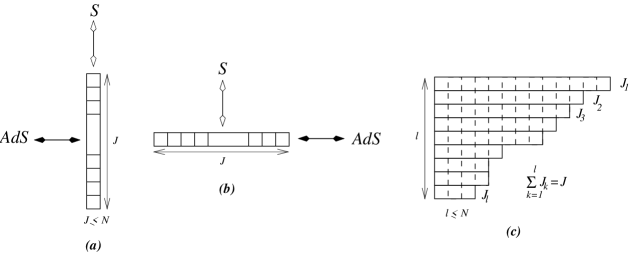
Figure 4: Some Young Tableaux with $J$ boxes. (a) A totally anti-symmetric representation. This corresponds to a single giant graviton of radius $\sqrt{J}$ grown in $S^{5}$ or $J$ tiny gravitons residing in $AdS_{5}$. (b) A totally symmetric representation which corresponds to a single giant graviton in $AdS_{5}$ or $J$ tiny gravitons in $S^{5}$. (c) A generic Young tableau of $l$ rows and $J$ boxes. If we view the tableaux from above (focusing on columns) we see giants grown in $S^{5}$, and if we view it from the left side (focusing on rows) we see giants in $AdS_{5}$. In a $U(N)$ Young tableau number of rows cannot exceed $N$, a realization of the stringy exclusion principle [12]. From the viewpoint of giants grown in $AdS$, however, this is the number of concentric 3-branes, and not their size, which cannot exceed $N$. The fact that each Young tableau has two interpretations in terms of giants in $S^{5}$ or $AdS_{5}$ is a manifestation of particle-hole duality in the two dimensional fermion picture discussed in [13].

On the other hand there is a one-to-one correspondence between partitions of $J$ into arbitrary positive integers and the representations of ${\cal S}_{J}$. Hence it is evident that there is a one-to-one correspondence between our generic fuzzy sphere solutions of section 3.2.3 and the Young Tableaux with $J$ boxes. In this point of view each box in the Young tableau corresponds to a tiny graviton.

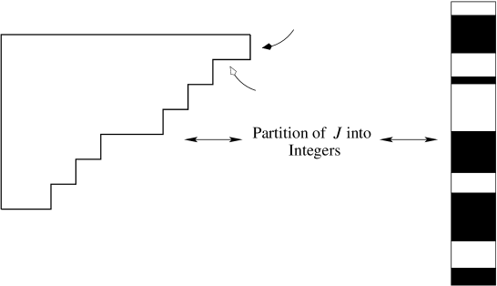
Figure 5: A Young tableau of $J$ boxes has three interpretations. i) A representation of $U(N)$, ii) Schur Polynomials and representation of permutation group ${\cal S}_{J}$ and iii) Partition of $J$ into non-negative integers. The first two interpretations were noticed in [13, 14, 30] as discussed there, they lead to an equivalent description of all 1/2 BPS configurations of ${\cal N}=4$ $U(N)$ SYM in terms of two dimensional fermion system. The third one, however, is the one, is relevant to the 1/2 BPS solutions of the TGMT.

We would also like to briefly comment on the relation to the supergravity solutions corresponding to the above 1/2 BPS states, recently constructed by Lin-Lunin-Maldacena [13]. However, first we need to review another equivalent description of the 1/2 BPS opterators of the ${\cal N}=4$ $U(N)$ gauge theory: A system of $N$ two dimensional fermions in harmonic oscillator potential. To see this recall that the part of the ${\cal N}=4$ $U(N)$ gauge theory on $R\times S^{3}$, relevant for the dynamics of chiral primary operators, in the temporal gauge, takes a very simple form:

$$S=\frac{1}{g^{2}_{YM}}\int d\tau\ Tr\left(\partial_{\tau}Z^{\dagger}\partial_{\tau}Z-Z^{\dagger}Z\right)\ .$$ (4.3)

The simplifications leading to the above action come from two sources: 1) the chiral primaries, among all the fields present in a ${\cal N}=4$ gauge multiplet, only involve $Z$’s and; 2) to be 1/2 BPS they should be invariant under $SO(4)$ acting on $S^{3}$ that the gauge theory is defined on. Therefore, we can perform integration over the $S^{3}$ to remain with a one dimensional action (4.3). The mass term for $Z$ is the conformal mass present for all of six scalars (and fermions) of the ${\cal N}=4$ SYM on $R\times S^{3}$. The action (4.3) which governs the dynamics of the chiral primary operators is nothing but the action for a bunch of decoupled harmonic oscillators all with the same frequency (note that $Z$’s are $N\times N$ matrices). One can still use the (global) $U(N)$ gauge transformations to bring $Z$’s to a diagonal form. These $N$ eigenvalues can directly be related to physical gauge invariant operators. In fact the eigenvalues correspond to position of $N$ two dimensional fermions in a harmonic oscillator potential. (If we choose to work with diagonal matrices, we should then add the Van der monde determinant, which in turn leads to the fermionic nature of the eigenvalues [31].)

In the two dimensional fermions viewpoint every chiral primary corresponds to a distribution of fermions or a “droplet” in the fermion phase space. In a recent work Lin-Lunin-Maldacena (LLM) [13] have constructed the supergravity solutions corresponding to each droplet. That is, they have shown that there is a one-to-one map between the 1/2 BPS type IIB supergravity solutions with $PSU(2|2)\times PSU(2|2)\times U(1)$ supersymmetry and the $N$ 2d fermion phase space. These solutions, as supergravity solutions, correspond to various classical giant gravitons in the $AdS_{5}\times S^{5}$ or the plane-wave background. We have discussed that there is a one-to-one correspondence between our 1/2 BPS solutions and the ${\cal N}=4$ gauge theory, hence we expect that our multi-fuzzy sphere solutions to be associated with the quantized LLM backgrounds. It is, however, hard to directly construct classical background metrics corresponding to a given Matrix theory configurations. This is also the case for BFSS Matrix Theory or its variants. Nonetheless, it should be possible to extract some information about the blackholes and their entropy from the matrix theory. We hope to address this question in future works.

5 Relation to Mass Deformed $D=3,\ {\cal N}=8$ SCFT

As discussed in [1] and reviewed in section 2, the TGMT Hamiltonian is obtained from quantization (discretization) of a 3-brane Hamiltonian in the plane-wave background, once the light-cone gauge is fixed. In the process of quantization, we prescribed to replace the classical Nambu 3-brackets, which naturally appear in the 3-brane action, with quantized Nambu 4-brackets. For that, however, we need to introduce a given fixed matrix, ${\cal L}_{5}$. In this section we intend to clarify the role and physical significance of the ${\cal L}_{5}$ and justify our prescription for quantization of Nambu 3-brackets.

In order that we recall the standard string/M-theory dualities and that type IIB string theory is related to M-theory on a $T^{2}$, under which an M5-brane (wrapping the $T^{2}$) is mapped to a D3-brane. On the other hand, the TGMT is a quantized 3-brane theory. Therefore, we propose that:

The TGMT can also be thought as a quantized M5-brane theory, ${\cal L}_{5}$ is indeed the reminiscent of the 11^th circle and the three sphere giants are M5-branes with the worldvolume ${\mathbb{R}}^{2+1}\times S^{3}$. The ${\mathbb{R}}^{2}$ part is in fact compactified over the $T^{2}$ which relates M and type IIB theories, one of the directions in $T^{2}$ is then along the ${\cal L}_{5}$ and the other one is along the $X^{-}$ direction.

    Evidence for the proposal

To present some pieces of evidence in support of the above proposal we first, very briefly, review the results and arguments of Bena-Warner [32], which may also be found in [13], where a class of 1/2 BPS solutions to 11 dimensional supergravity has been constructed. These solutions asymptote to $AdS_{4}\times S^{7}$ and, as discussed in [32], correspond to M2-branes dielectrically polarized into M5-branes. In these solutions the $S^{7}$ has been deformed in such a way that its $SO(8)$ isometry is reduced to $SO(4)\times SO(4)$. Physically these solutions correspond to (near horizon geometry of) a stack of M2-branes along $X^{0},X^{1},X^{2}$ directions and M5-branes along $X^{0},X^{1},X^{2}$ while their other three directions wrap an $S^{3}$ in the directions transverse to the M2-branes. Hence, the worldvolume of the M5-branes is on ${\mathbb{R}}^{2+1}\times S^{3}$. From the gravity viewpoint this deformed $AdS_{4}\times S^{7}$ is obtained by turning on a four-form flux through either of the $S^{3}$’s and the other remaining direction in $S^{7}$. (In our analysis we take this ${\mathbb{R}}^{2}$ to be compactified on an $S^{1}\times S^{1}$.) Due to the existence of the four-form flux one of this $S^{1}$ directions combine with one of the $S^{3}$’s to topologically form an $S^{4}$; the M5-branes then wrap the other $S^{3}$ [13].

This deformation of $AdS_{4}\times S^{7}$ has a dual description in terms of mass deformed three dimensional ${\cal N}=8$ SCFT. The mass deformation, which corresponds to the four-form flux through the $S^{3}$ in the supergravity solution, breaks the $SO(8)$ $R$-symmetry of the SCFT to a $SO(4)\times SO(4)$ subgroup, as well as half of the supersymmetry.

The isometries of this solution include two translations along the M2-brane worldvolume. Following [32, 13], one may U-dualize this solution along this ${\mathbb{R}}^{2}$ down to type IIB supergravity. In the type IIB, however, the M5-branes appear as three sphere giant gravitons. One of the U-duality directions after the duality appear as the $X^{-}$ direction in our ten dimensional plane-wave background. In our DLCQ description this direction is compact with the radius $R_{-}/\mu$ (in units of $l_{s}$). We propose that the other one has a non-trivial appearance in our TGMT Hamiltonian through the ${\cal L}_{5}$. In other words, the TGMT already knows about the 11 dimensional origin of the type IIB string theory.

As the first piece of evidence recall that, as we discussed and emphasized in section 3.1, a fuzzy three sphere which is a quantized three sphere giant, is topologically a four sphere. The ${\cal L}_{5}$, which is the reminiscent of the (fuzzy) four sphere we started with, has a non-vanishing extent, cf. Figure 1. The non-zero extent of ${\cal L}_{5}$ is a “quantum” effect and therefore the 11 dimensional origin of the TGMT is a result of quantization of type IIB string theory. Recalling that ${\cal L}_{5}\sim l/R$, in the classical limit, $l\to 0$, $R$=fixed, ${\cal L}_{5}$ goes to zero and hence we reproduce the usual ten dimensional type IIB theory.

As a more quantitative evidence, we note the relation between the fuzziness, $g_{s}$ and $R_{-}$ (2.7), which can be written as

$$g_{s}=\frac{{R_{-}}/{\mu}}{{l^{2}}/{l_{s}^{2}}}.$$ (5.1)

The above should be compared with the expression for the coupling of type IIB string theory obtained from M-theory on $T^{2}$. If the radii of the two cycles in $T^{2}$ are $R_{1},R_{2}$, then $g_{s}=R_{1}/R_{2}$, e.g. see [33]. If we identify $R_{1}$ with $R_{-}/\mu$, then (5.1) implies that $R_{2}=l^{2}/l_{s}^{2}$.

Next, we note that as a direction in a fuzzy four sphere the width of the ${\cal L}_{5}$ strip in units of $l_{s}$ is $\delta X^{5}=L{\cal L}_{5}\sim Ll/R$, where $L^{4}$ is the smallest volume one can measure on an $S^{4}_{f}$, cf. discussions at the end of Appendix B. Using (B.28) we have

$$\delta X^{5}=\frac{lR}{l_{s}^{2}}\cdot\frac{l}{R}=\frac{l^{2}}{l_{s}^{2}}\ ,$$ (5.2)

which is what we expected for $R_{2}$ from a $T^{2}$ compactification of M-theory. This is a remarkable result because reproduction of the standard string/M-theory dualities and their implications is among the strong supportive evidence for the TGMT conjecture.

6 Discussion and Outlook

As a start to a detailed analysis of the tiny graviton matrix theory (TGMT), in this paper we studied the zero energy 1/2 BPS configurations of the theory. These solutions are labeled by reducible or irreducible $J\times J$ representations of $SO(4)$ and physically correspond to various giant gravitons of different size, extended in $X^{i}$ and/or $X^{a}$ directions.

Recently there have been an interest in better understanding of similar 1/2 BPS configurations in the context of usual AdS/CFT correspondence in both gauge theory [14] and gravity [13] sides. The interest in the 1/2 BPS configurations is motivated by the fact that these 1/2 BPS states may help us with pushing the analysis of AdS/CFT to beyond the supergravity limit. In this respect our analysis parallels these studies, though in the context of the TGMT which is conjectured to be a non-perturbative, exact description of DLCQ of type IIB strings on $AdS_{5}\times S^{5}$. Of course, analysis of the 1/2 BPS states is a part of a bigger problem, which has been depicted in Figure 6. In [1] and also in this work we have tried to, at least, start addressing the AdS-TGMT-CFT triality. In this direction we have noted that a Young tableau can simultaneously label all the 1/2 BPS states/configurations of the ${\cal N}=4,D=4$ $U(N)$ SYM, type IIB supergravity [13] and also TGMT, see Figure 5. It is very desirable to expand our understanding of the triality, which is postponed to future works. One interesting question is whether the two dimensional fermions of [13, 14] has a closer relation to the tiny gravitons [20]. Among the points and puzzles to be understood in this direction we should mention the fact that size of the matrices corresponding to a single fuzzy sphere solution, $J$, is fixed once we identify a quantum giant graviton as a fuzzy three sphere. In particular $J$ cannot take any arbitrary value (cf. eq.(3.16)). This rises the puzzle that in the gauge theory we can have e.g. subdeterminant operators with arbitrary length (or R-charge). Resolution of this puzzle is postponed to a future work [20].

Figure 6: The AdS-TGMT-CFT triality

One of the basic ingredients used in the formulation of TGMT is the fact that the gauge symmetry of $m$ coincident giant gravitons, similarly to the flat D-branes, is $U(m)$. There have been two independent arguments in support of this property [17, 18]. Noting a generic Young tableau we already see strong indications for this, see Figure 7. It is, however, instructive to re-derive the same fact from the TGMT. As the first step in this direction one may start with working out a configuration in TGMT corresponding to the giant hedge-hogs of [17], the “fuzzy giant hedge-hogs”.

Figure 7: The “fluctuations” above the Young tableau corresponding to $n$ coincident giants in $AdS$ or $m$ coincident giants in $S^{5}$ can be thought as a Young tableau for states in a $U(n)$ or $U(m)$ gauge theory.

As we have seen so far giant gravitons, and not fundamental strings of type IIB, naturally appear in the TGMT. The first question to ask is where are the type IIB fundamental strings. In [1] there was a proposal that the $X=0$ vacuum corresponds to single string vacuum, around which fundamental strings appear as non-perturbative objects. In addition to the single string vacuum, we need to work out the details of multi-string vacua. Moreover, as TGMT is a formulation of type IIB string theory with compact $X^{-}$ direction, to specify the string vacuum states besides the light-cone momentum we should also give the winding number. Besides the vacuum states it is interesting to make connection between the TGMT description of type IIB strings on the ten dimensional plane-wave and the string bit model of Verlinde [34].

In section 2 we gave an argument that the classical size of a tiny graviton is $l$. Through a detailed analysis of the fuzzy three sphere solutions, however, we found that quantum mechanically the smallest volume that one can probe on an $S^{3}_{f}$ is in principle much larger than $l^{4}$, that is $L^{4}$ (B.28). It is interesting to compare $L$ with the ten dimensional Planck length $l_{p}$. Combining, (2.3), (B.28) and (3.19) we obtain

$$L^{2}=\sqrt{\frac{J}{N}}l^{2}_{p}\ .$$ (6.1)

When the stringy exclusion relation discussed in [12] is saturated, i.e. $J\sim N$, $L\sim l_{p}$ and hence in this case $l_{p}$ is indeed the smallest physical length that one can probe.

In constructing our solutions we used an embedding of the fuzzy three spheres in $\mathbb{C}^{4}_{\theta}\times\mathbb{C}^{4}_{\theta}$. It is amusing to see whether these two copies of the eight dimensional Moyal plane are just mathematical tools or have a more physical meaning. As a relevant point we note that the minimal physical length scale of the TGMT is $L$ which is equal to the noncommutativity scale on these Moyal planes (B.29).

In the Appendix B.2.2 we reviewed and elaborated on a new method of construction of fuzzy spheres based on embedding them into higher dimensional Moyal planes. This method works perfectly well for the cases where the sphere admits a Hopf fibration. There are, however, only four such possibilities somehow related to the fact that the division algebras are only limited to real ${\mathbb{R}}$, complex $\mathbb{C}$, quaternion ${\mathbb{H}}$ and octonions ${\mathbb{O}}$. Among these cases we have used the first three and only the last one, which leads to a Hopf fibration of an $S^{15}$ with an $S^{8}$ base is remaining. One may use this and discussions of B.2.2 to construct a description of $S^{8}_{f}$ and $S^{7}_{f}$ by embedding them into a $\mathbb{C}^{8}_{\theta}$.

As discussed in section 5 the TGMT is related to a mass deformed $D=3,{\cal N}=8$ SCFT, which in turn is also related to specific deformations of the $D=6$ $(0,2)$ SCFT. (The latter can be understood because in the Bena-Warner solutions [32], besides a stack of M2-branes we have M5-branes with worldvolume ${\mathbb{R}}^{2+1}\times S^{3}$.) Unfortunately we do not have an action for neither of the three and six dimensional SCFTs. Recently there has been a proposal for obtaining an action for the $D=3$ SCFTs [35]. In view of the above connections, it is an interesting problem to check if TGMT and/or the idea of quantized Nambu $p$-brackets can help with finding an action for either of the two SCFTs.

Appendix A Conventions and Identities

In our construction of the fuzzy four sphere, $S^{4}_{f}$, which will be reviewed in the next Appendix, we need to develop some identities involving $spin(5)$ gamma matrices. These are essentially the usual four dimensional Dirac matrices which obey the anticommutation relation, Clifford algebra

$$\left\{\gamma_{i},\gamma_{j}\right\}=2\delta_{ij}{\bf 1_{4\times 4}}\ ,\ \ \ \ \ \ i,j=1,2,3,4.$$ (A.1)

We follow the conventions in which the Dirac gamma matrices are

$$\gamma^{i}=\left(\begin{matrix}0&&\sigma^{i}\\ \bar{\sigma}^{i}&&0\end{matrix}\right),\ \gamma^{5}=\left(\begin{matrix}\mathbf{-1_{2\times 2}}&&0\\ 0&&\mathbf{1_{2\times 2}}\end{matrix}\right),\ \mathbf{1_{4\times 4}}=\left(\begin{matrix}\mathbf{1_{2\times 2}}&&0\\ 0&&\mathbf{1_{2\times 2}}\end{matrix}\right).$$ (A.2)

where

$$\sigma^{i}=(\mathbf{1_{2\times 2}},-i\vec{\sigma}_{pauli}),\ \bar{\sigma}^{i}=(\mathbf{1_{2\times 2}},i\vec{\sigma}_{pauli})$$ (A.3)

with the $\vec{\sigma}_{pauli}$ being the standard Pauli sigma matrices:

$$\sigma^{1}=\left(\begin{matrix}0&&1\\ 1&&0\end{matrix}\right),\ \sigma^{2}=\left(\begin{matrix}0&&-i\\ i&&0\end{matrix}\right),\ \sigma^{3}=\left(\begin{matrix}1&&0\\ 0&&-1\end{matrix}\right),\ \mathbf{1_{2\times 2}}=\left(\begin{matrix}1&&0\\ 0&&1\end{matrix}\right)\ .$$ (A.4)

In (A.2) $\gamma^{5}=\gamma^{1}\gamma^{2}\gamma^{3}\gamma^{4}=\frac{1}{4!}\epsilon_{ijkl}\gamma^{i}\gamma^{j}\gamma^{k}\gamma^{l}$.

In our conventions,

$$2\gamma^{ij}\equiv[\gamma^{i},\gamma^{j}]=\left(\begin{matrix}\sigma^{ij}&&0\\ 0&&\bar{\sigma}^{ij}\end{matrix}\right),\qquad\gamma^{i}\gamma^{5}=\left(\begin{matrix}0&&-\sigma^{i}\\ \bar{\sigma}^{i}&&0\end{matrix}\right)$$

and also

$$[\gamma^{i},\gamma^{j}\gamma^{5}]=2\delta^{ij}\gamma^{5}\ ,$$ (A.5)

where

$$\sigma^{ij}\equiv\sigma^{i}\bar{\sigma}^{j}-\sigma^{j}\bar{\sigma}^{i}, \bar{\sigma}^{ij}\equiv\bar{\sigma}^{i}\sigma^{j}-\bar{\sigma}^{j}\sigma^{i}$$

$$\sigma^{i}\bar{\sigma}^{j}+\sigma^{j}\bar{\sigma}^{i}=2\delta^{ij}, \bar{\sigma}^{i}\sigma^{j}+\bar{\sigma}^{j}\sigma^{i}=2\delta^{ij}\ .$$

$\gamma^{ij}$’s constitute a $4\times 4$ representation for the generators of the $spin(4)$ algebra. If we add $\gamma^{i}\gamma^{5}$ to this collection, we have a representation of $spin(5)$; and the set of $\{\gamma^{ij},\ \gamma^{i}\gamma^{5},\ \gamma^{i},\gamma^{5}\}$ would give the representation of the $spin(6)=su(4)$ algebra.

Next we list some useful identities involving $\sigma^{i}$ and $\bar{\sigma}^{i}$:

$$\frac{1}{2}\epsilon^{ijkl}\sigma^{ij}=\epsilon^{ijkl}\sigma^{i}\bar{\sigma}^{j}=+\sigma^{kl}\ \ ,\qquad\frac{1}{2}\epsilon^{ijkl}\bar{\sigma}^{ij}=\epsilon^{ijkl}\bar{\sigma}^{i}\sigma^{j}=-\bar{\sigma}^{kl}$$ (A.6)

$$(\sigma^{i})_{\alpha\beta}(\sigma^{i})_{\lambda\rho}=(\bar{\sigma}^{i})_{\alpha\beta}(\bar{\sigma}^{i})_{\lambda\rho} = +2(\delta_{\alpha\beta}\delta_{\lambda\rho}-\delta_{\alpha\rho}\delta_{\beta\lambda})$$

$$(\sigma^{i})_{\alpha\beta}(\bar{\sigma}^{i})_{\lambda\rho}=(\bar{\sigma}^{i})_{\alpha\beta}(\sigma^{i})_{\lambda\rho} = +2\delta_{\alpha\rho}\delta_{\beta\lambda}$$ (A.7)

$$(\sigma^{ij})_{\alpha\beta}(\sigma^{i})_{\gamma\lambda} = +2(\delta_{\gamma\lambda}\bar{\sigma}^{j}_{\alpha\beta}-\delta_{\alpha\lambda}\bar{\sigma}^{j}_{\gamma\beta}-\delta_{\beta\gamma}\sigma^{j}_{\alpha\lambda})$$

$$(\bar{\sigma}^{ij})_{\alpha\beta}(\bar{\sigma}^{i})_{\gamma\lambda} = +2(\delta_{\gamma\lambda}\sigma^{j}_{\alpha\beta}-\delta_{\alpha\lambda}\sigma^{j}_{\gamma\beta}-\delta_{\beta\gamma}\bar{\sigma}^{j}_{\alpha\lambda})$$ (A.8)

$$(\sigma^{ij})_{\alpha\beta}(\bar{\sigma}^{i})_{\gamma\lambda} = -2(\delta_{\gamma\lambda}\sigma^{j}_{\alpha\beta}-\delta_{\alpha\lambda}\bar{\sigma}^{j}_{\gamma\beta}-\delta_{\beta\gamma}\sigma^{j}_{\alpha\lambda})$$

$$(\bar{\sigma}^{ij})_{\alpha\beta}(\sigma^{i})_{\gamma\lambda} = -2(\delta_{\gamma\lambda}\bar{\sigma}^{j}_{\alpha\beta}-\delta_{\alpha\lambda}\sigma^{j}_{\gamma\beta}-\delta_{\beta\gamma}\bar{\sigma}^{j}_{\alpha\lambda})$$

$$(\sigma^{ij})_{\alpha\beta}(\sigma^{ij})_{\gamma\lambda}=(\bar{\sigma}^{ij})_{\alpha\beta}(\bar{\sigma}^{ij})_{\gamma\lambda} = 16(\delta_{\alpha\beta}\delta_{\gamma\lambda}-2\delta_{\alpha\delta}\delta_{\gamma\beta})$$ (A.9)

$$(\sigma^{ij})_{\alpha\beta}(\bar{\sigma}^{ij})_{\gamma\lambda}=(\bar{\sigma}^{ij})_{\alpha\beta}(\sigma^{ij})_{\gamma\lambda} = 0$$

Appendix B Nambu Brackets and Fuzzy Spheres

As fuzzy spheres are the crucial ingredients in our solutions to the zero energy half BPS configurations of the tiny graviton matrix theory in this appendix we present a brief review on the fuzzy spheres. There are two equivalent approaches for the construction of fuzzy spheres. The first, which also historically came earlier, is based on finding finite dimensional representations of $SO(d+1)$ (more precisely $spin(d+1)$) for a fuzzy $d$-sphere, $S^{d}_{f}$. This construction was first proposed for a two sphere [36] and then extended to four [23] and to higher dimensional spheres [25]. The second construction which were first introduced and emphasized in [1] is more geometrical, and is based on the “quantization” of the “Nambu brackets” [37]. Nambu brackets encode the isometries of the spheres. That is this second method which paves the way for the quantization of the giant gravitons, which in turn leads to the matrix theory description of the DLCQ of string/M- theory on the plane-wave backgrounds [1]. Hence, in B.1 we review Nambu brackets which are generalized form of the Poisson bracket and prescribe a consistent way to quantize them. In B.2, using the definition of round spheres through Nambu brackets we present the definition of fuzzy spheres and then try to construct explicit solutions for the fuzzy two and four sphere cases.

B.1 Nambu brackets

In this subsection we give the definition of Nambu brackets and prescribe how to quantize them consistently to make multilinear commutators.

Classical Nambu $p$-brackets

A Nambu $p$-bracket is defined among $p$ functions ${\cal F}_{i}(\sigma^{r}),r,p=1,\dots,p$ as

$$\left\{{\cal F}_{1},{\cal F}_{2},\dots,{\cal F}_{p}\right\}\equiv\epsilon^{r_{1}r_{2}\cdots r_{p}}\frac{\partial{\cal F}_{1}}{\partial\sigma^{r_{1}}}\frac{\partial{\cal F}_{2}}{\partial\sigma^{r_{p}}}\dots\frac{\partial{\cal F}_{p}}{\partial\sigma^{r_{p}}}\ ,$$ (B.1)

where ${\cal F}_{i}$ are functions on a $p$-dimensional space parameterized by $\sigma^{r}$. Obviously for $p=2$ (B.1) reduces to the standard Poisson bracket. These brackets, as enumerated in [1], have five important properties: cyclicity, (generalized) Jacobi identity, associativity, trace and by-part integration properties.

Quantization of Nambu $p$-brackets

In order to pass to quantum (fuzzy, discretized or noncommutative) physics, we generalize the standard prescription, namely start from Hamilton-Jacobi formalism, substitute functions of phase space coordinates with operators (matrices) acting on Hilbert space, the Nambu brackets with multilinear commutators (quantized Nabmu brackets) and integrals with trace, i.e.

$${\cal F}\longleftrightarrow\hat{{\cal F}}\qquad ;\qquad\int d^{p}\sigma\longleftrightarrow Tr$$ (B.2a)

$$\left\{{\cal F}_{1},\cdots,{\cal F}_{p}\right\}\longleftrightarrow\frac{1}{(i\hbar)^{p/2}}[\hat{{\cal F}}_{1},\cdots,\hat{{\cal F}}_{p}] \equiv\frac{1}{(i\hbar)^{p/2}}\epsilon^{i_{1}\cdots i_{p}}\hat{{\cal F}}_{i_{1}}\hat{{\cal F}}_{i_{2}}\cdots\hat{{\cal F}}_{i_{p}}$$ (B.2b)

This prescription only works for even dimensional spaces ($p=2k$), more precisely, for even case commutators it has the crucial properties of the Nambu brackets we mentioned above, that is cyclicity, generalized Jacobi identity and by-part and trace property. Note, however, that with (B.2b) we have lost associativity [38, 1].

As for the odd case ($p=2k-1$), besides the associativity we also lose the physically very important trace and by-part integration properties. To overcome that problem, in [1] it was proposed to replace an odd $p$-bracket with an even $(p+1)$-bracket and then again use (B.2b). In order that, we should introduce a fixed matrix, a non-dynamical operator, ${\cal L}_{2k+1}$ (at least in string theory and in the case of fuzzy odd spheres we have strong evidence where it comes from, e.g. see discussions of [1] and also section 5). The prescription for quantization of odd brackets is then

$${\cal F}\longleftrightarrow\hat{{\cal F}}\ ;\ \left\{{\cal F}_{1},\cdots,{\cal F}_{2k-1}\right\}\longleftrightarrow\frac{1}{(i\hbar)^{k}}\left[\hat{{\cal F}}_{1},\cdots,\hat{{\cal F}}_{2k-1},{\cal L}_{2k+1}\right]\ ;\ \int d^{2k-1}\sigma\longleftrightarrow Tr\ .$$ (B.3)

B.2 Fuzzy spheres

Any round (classical, continuous, commutative) $d$-sphere with radius $R$ should satisfy these constraints as defining properties

$$\sum_{\mu=1}^{d+1}(X^{\mu})^{2}=R^{2}\qquad;\qquad\{X^{\mu_{1}},X^{\mu_{2}},\cdots,X^{\mu_{d}}\}=R^{d-1}\epsilon^{\mu_{1}\cdots\mu_{d+1}}X^{\mu_{d+1}}.$$ (B.4)

The $d+1$ embedding coordinates $X^{\mu}$ rotate as a vector under the isometry symmetry of the $d$-sphere, $SO(d+1)$. In fact the bracket equation in (B.4) is a manifestation of the $SO(d+1)$ isometry. (Note that $SO(d+1)$ has only two invariant tensors, the metric $\delta_{\mu\nu}$ and $\epsilon^{\mu_{1}\cdots\mu_{d+1}}$.)

In order to pass to the fuzzy (discretized or noncommutative) $d$-sphere, we follow the prescription for quantizing Nambu brackets presented above. Let us first start with a fuzzy even sphere. A fuzzy $2k$ sphere, $S^{2k}_{f}$, is defined through

$$\sum_{\mu=1}^{2k+1}(X^{\mu})^{2}=R^{2}\qquad;\qquad\left[X^{\mu_{1}},X^{\mu_{2}},\cdots,X^{\mu_{2k}}\right]=i^{k}\lambda^{2k-1}\epsilon^{\mu_{1}\mu_{2}\cdots\mu_{2k+1}}X^{\mu_{2k+1}},$$ (B.5)

which leads to

$$\epsilon^{i_{1}i_{2}\cdots i_{2k+1}}X^{i_{1}}X^{i_{2}}\cdots X^{i_{2k+1}}=i^{k}\lambda^{2k-1}R^{2}.$$

In the above, we have defined the “${\hbar}$” (cf. (B.2b)) as $(\lambda/R)^{(2k-1)/k}$ and $\lambda$, which in a sense quantifies how much our sphere is far from the classical sphere, will be called the “fuzziness”.

Similarly for the fuzzy odd-spheres

$$\sum_{i=1}^{2k}(X^{i})^{2}=R^{2}\qquad;\qquad\left[X^{i_{1}},X^{i_{2}},\cdots,X^{i_{2k-1}},{\cal L}_{2k+1}\right]=i^{k}l^{2(k-1)}\epsilon^{i_{1}i_{2}\cdots i_{2k}}X^{i_{2k}}$$ (B.6)

leading to

$$\epsilon^{i_{1}i_{2}\cdots i_{2k+1}}X^{i_{1}}X^{i_{2}}\cdots{\cal L}_{2k+1}X^{i_{2k}}=i^{k}l^{2(k-1)}R^{2}.$$

With the above definition, the problem of construction of fuzzy even spheres is now reduced to finding explicit solutions to (B.5) in terms of some $N\times N$ matrices and giving the relation between the size of the sphere (its radius) and the size of the matrices. For the fuzzy odd sphere case, in addition we should also give an appropriate ${\cal L}_{2k+1}$. Note that by construction, solutions to (B.5) or (B.6) are only specified up to an $SO(d+1)$ rotation:

$${\cal R}_{ij}X^{j}=U({\cal R})X_{i}U({\cal R})^{-1},$$

where ${\cal R}_{ij}$ are the generators of the $spin(d+1)$ isometry group of the sphere and $U({\cal R})$ are an $N\times N$ representation of ${\cal R}$.

In this appendix, as examples, we will construct explicit solutions to (B.5) for $k=1,2$ cases, i.e. fuzzy two and four spheres. The construction of $S^{3}_{f}$ is presented in section 3 of the main text. There are two ways to solve these equations and realize the fuzzy spheres, group theoretical and harmonic oscillator approaches. The first approach is widely studied and used since the introduction of fuzzy spheres was based on the group and the representation theory of the isometry of the sphere under study. The harmonic oscillator approach is a less-known one and is well-suited for specific dimension, and is inspired by principal Hopf fibrations. This method for the fuzzy two sphere were studied in some detail in [22].

B.2.1 Group theoretical construction of fuzzy spheres

The fuzzy $2k$-sphere is defined through the algebra ${\cal M}_{N}$ of $N\times N$ hermitian matrices. When $N\rightarrow\infty$ the corresponding matrix geometry tends to the geometry of the round $2k$-sphere. To realize this idea, we think of the ordinary geometry of the round sphere as an infinite dimensional representation of $spin(2k+1)$ algebra. To pass to the fuzzy case, however, we need finite dimensional representations. Due to the basic theorem of the algebraic geometry, one can replace a given manifold with the algebra of functions defined on that. For the case of the $S^{2k}$ that is the algebra ${\cal F}$ of functions $f(X^{\mu})$ on $S^{2k}$ which admits a polynomial expansion in the $X^{\mu}$’s:

$$f(X_{\mu})=f_{0}+f_{\mu}X^{\mu}+\frac{1}{2}f_{\mu\nu}X^{\mu}X^{\nu}+\frac{1}{6}f_{\mu\nu\rho}X^{\mu}X^{\nu}X^{\rho}+\cdots$$ (B.7)

Now we would like to truncate this expansion in such a way that it is convertible to an algebra. To turn this approximation to algebra we replace $X^{\mu}$ with generalized gamma matrices ${\cal G}^{\mu}_{2k}$ of the algebra ${\cal M}_{N_{k}(n)}$ of $N_{k}(n)\times N_{k}(n)$ hermitian matrices. These matrices are defined as follows

$${\cal G}^{\mu} = (\Gamma^{\mu}\otimes\mathbf{1}\otimes\cdots\otimes\mathbf{1}+\mathbf{1}\otimes\Gamma^{\mu}\cdots\otimes\mathbf{1}+\cdots+\mathbf{1}\otimes\cdots\mathbf{1}\otimes\Gamma^{\mu})_{Sym}$$ (B.8)

$${\cal G}^{\mu\nu} = (\Gamma^{\mu\nu}\otimes\mathbf{1}\otimes\cdots\otimes\mathbf{1}+\mathbf{1}\otimes\Gamma^{\mu\nu}\cdots\otimes\mathbf{1}+\cdots+\mathbf{1}\otimes\cdots\mathbf{1}\otimes\Gamma_{\mu\nu})_{Sym}$$ (B.9)

where ${\cal G}^{\mu\nu}=\frac{1}{2}\left[{\cal G}^{\mu},{\cal G}^{\nu}\right]$ and $\Gamma^{\mu\nu}=\frac{1}{2}\left[\Gamma^{\mu},\Gamma^{\nu}\right]=\Gamma^{\mu}\Gamma^{\nu}$ are the generators of $SO(2k+1)$. These generalized gamma matrices are $n$-fold direct tensor-product of gamma matrices and identity matrix and the symmetrization means that they are defined on the vector space $Sym\left(V^{\otimes n}\right)$, the symmetrized $n$-fold tensor product space of the smallest irreducible representation of $spin(2k+1)$, $V$; and $dim(Sym\left(V^{\otimes n}\right))=N(n)$. Hence, ${\cal G}^{\mu}$ are $N\times N$ matrices. These matrices have following properties

$$\sum_{\mu=1}^{2k+1}{\cal G}_{\mu}{\cal G}_{\mu} =n(n+2k)\ ,$$ (B.10a)

$$\left[{\cal G}^{\mu_{1}},{\cal G}^{\mu_{2}},\dots,{\cal G}^{\mu_{2k}}\right] =-(-i)^{k}(2k)!!(2k-2+n)!!\epsilon^{\mu_{1}\mu_{2}\cdots\mu_{2k+1}}{\cal G}^{\mu_{2k+1}}.$$ (B.10b)

If we now define $X_{\mu}=\tilde{\lambda}{\cal G}^{(2k)}_{\mu}$ we can see that this matrix construction truly gives $S_{f}^{2k}$. The only remaining step to complete the construction is then to specify $N$ as a function of $n$, which in turn, noting (B.10), gives the relation between the size of matrices $N$ and the radius of the fuzzy sphere $R$. We will work this out for two specific cases of $S^{2}_{f}$ and $S^{4}_{f}$.
Construction of $S_{f}^{2}$

Here we deal with $spin(3)=SU(2)$, and hence the analog of (B.8) for this case is the generalized Pauli sigma matrices,

$$\Sigma_{i}=(\sigma_{i}\otimes\mathbf{1}\otimes\cdots\otimes\mathbf{1}+\mathbf{1}\otimes\sigma_{i}\otimes\cdots\otimes\mathbf{1}+\cdots+\mathbf{1}\otimes\cdots\otimes\mathbf{1}\otimes\sigma_{i})_{Sym}\ ,$$ (B.11)

where $\sigma^{i}$ are $2\times 2$ Pauli matrices. $\Sigma_{i}$ form an $(n+1)\times(n+1)$ representation of the $SU(2)$ algebra, corresponding to spin $n/2$ states. Note that for $SU(2)$

$$N\equiv dim(Sym(V^{\otimes}))=n+1\ .$$ (B.12)

The embedding coordinates can be identified as $X^{i}=\frac{\lambda}{2}\Sigma^{i}$. The size of the matrices and the radius of the sphere are then related as

$$R^{2}_{S^{2}_{f}}=\frac{\lambda^{2}}{4}(N^{2}-1).$$ (B.13)

Construction of $S_{f}^{4}$

Here the basic $\gamma$-matrices we start with are the standard $4\times 4$ Dirac $\gamma$-matrices, together with $\gamma^{5}$, for our conventions see Appendix A. These $\gamma$ matrices satisfy

$$\sum_{\mu=1}^{5}\gamma^{\mu}\gamma^{\mu}=5\qquad;\qquad[\gamma^{\mu},\gamma^{\nu},\gamma^{\rho},\gamma^{\alpha}]=4!\epsilon^{\mu\nu\rho\alpha\beta}\gamma^{\beta}$$

Again one can use (B.8) to construct an $N\times N$ representation out of these $\gamma$’s. The only remaining part is how $N$ and the radius of the fuzzy four sphere are related. To work this out, one should use representation theory of $spin(5)$. This has been carried out in [25] and the result is $N=\frac{1}{6}(n+1)(n+2)(n+3)$, where $R^{2}_{S^{4}_{f}}\propto n(n+4)$.

B.2.2 Harmonic oscillator construction of fuzzy spheres

Commutative $d$-spheres are usually defined through embedding the $S^{d}$ in ${\mathbb{R}}^{d+1}$. The natural question to ask is whether a similar thing is also possible for a noncommutative fuzzy sphere. Precisely, the question is whether it is possible to embed an $S^{d}_{f}$ into a noncommutative plane, preferably a noncommutative Moyal plane. The answer, if positive, cannot be a $d+1$ dimensional plane. This can be seen from the fact that imposing the noncommutativity on the coordinates of the plane reduces the $SO(d+1)$ rotational invariance. Hence, we should look for embedding the $S^{d}_{f}$ into a higher dimensional Moyal plane, which includes $SO(d+1)$ among its isometries. In working with Moyal plane, it is more convenient to adopt complex coordinates. Let us consider a $\mathbb{C}^{p}$ space parameterized with the coordinates $z_{\alpha},\ \alpha=1,2,\cdots,p$ which satisfy the following commutation relation

$$[z_{\alpha},\bar{z}_{\beta}]=\theta\delta_{\alpha\beta}\ .$$ (B.14)

We denote this space by $\mathbb{C}^{p}_{\theta}$. (In terms of $a_{\alpha}=z_{\alpha}/\sqrt{\theta}$, the above is nothing but the algebra of a $p$ dimensional harmonic oscillator.) The idea is to solve (B.5) for an $S^{2k}_{f}$ using (B.14). The first thing to specify is what is the appropriate $p$ for a given $k$. For that we note that $\mathbb{C}^{p}_{\theta}$, and specifically (B.14), is invariant under $U(p)$ transformations which rotate $z_{\alpha}$ to $(U\ z)_{\alpha}$, $U\in U(p)$. Therefore, as the first criterion, $SO(2k+1)$ should be a subgroup of $U(p)$, e.g. for $k=1$, the case of a two sphere, $p$ can be two and for $k=2$, the four sphere case, $p$ should at least be four. For a generic case, one may start with

$$X^{\mu}=\kappa\bar{z}_{\alpha}\left(\Gamma^{\mu}\right)_{\alpha\beta}z_{\beta}\ ,$$ (B.15)

where $\Gamma^{\mu}$ are $2k+1$ dimensional Dirac matrices, and hence are $D\times D$ matrices, where $D$ is the dimension of the smallest fermionic representation of $SO(2k+1)$. As is evident from (B.15) the proper choice is $p=D$. For $k=1$ and $2$, $D=2^{2/2}=2$ and $2^{4/2}=4$. In (B.15) $\kappa$ is a parameter of dimension one over length.

We would like to use (B.15) as the relations embedding a sphere in Moyal plane. In (B.15) the $\Gamma^{\mu}$ matrices are essentially Clebsch-Gordon coefficients relating $U(p)$ vectors to $SO(2k+1)$ vectors. It is worth-noting that $X^{\mu}$’s defined in (B.15), similarly to the $\Gamma^{\mu}$’s, are hermitian and well-suited for our purpose.

As a warm-up let us first focus on the case of the fuzzy two sphere and then discuss the case of four sphere and possible generalizations to higher dimensional spheres.
Construction of $S^{2}_{f}$

We are looking for an embedding of an $S^{2}_{f}$ in a $C^{2}_{\theta}$. This is done in [22] and here we briefly review that. To start with, consider

$$X^{i}=\frac{\kappa}{2}\bar{z}_{\alpha}(\sigma^{i})_{\alpha\beta}z_{\beta}\ ,$$ (B.16)

where $i=1,2,3$ and $\alpha,\beta=1,2$. If $[z_{\alpha},\bar{z}_{\beta}]=\theta\delta_{\alpha\beta}$, it is straightforward to show that

$$[X^{i},X^{j}]=i\kappa\theta\ \epsilon_{ijk}X_{k}\ .$$ (B.17)

Furthermore, one can easily show that

$$\sum_{i=1}^{3}(X^{i})^{2}=\kappa^{2}\theta^{2}\ X^{0}(X^{0}+\bf 1),$$ (B.18)

where we have defined

$$X^{0}=\frac{1}{2\theta}\bar{z}_{\alpha}z_{\alpha}\ .$$

From (B.17) the fuzziness, $\lambda$, is identified as

$$\lambda=\kappa\theta\ ,$$ (B.19)

and hence

$$R^{2}_{S^{2}_{f}}=\lambda^{2}X^{0}(X^{0}+1).$$ (B.20)

It is noteworthy that $[X^{0},f(X^{i})]=0$, where $f$ is a generic function of $X^{i}$’s. If we choose $\kappa$, which is so far a free parameter, to be $1/\sqrt{\theta}$ then $\lambda=\sqrt{\theta}$. That is, the fuzziness is equal to the noncommutativity parameter of the embedding Moyal plane. (Note that the minimal area which one can measure in the Moyal plane is $\theta$.) Another interesting choice for $\kappa$ can be $1/R$. We will return to this choice and its physical significance later.

$X^{i}$ and $X^{0}$, as matrices are infinite dimensional, however, we are looking for finite dimensional matrices. In addition, in order to have a fuzzy two sphere (of a given radius) we need $\sum(X^{i})^{2}$ to be proportional to the identity matrix. Noting (B.18), this means that we should restrict $X^{0}$ to a block in which it is proportional to identity. This can be easily done, recalling that $X^{0}$ is the number operator for a two dimensional harmonic oscillator and hence in the number operator basis it takes a diagonal form, consisting of blocks $(n+1)\times(n+1)$ blocks with the eigenvalue $n$. (For a two dimensional harmonic oscillator the multiplicity of a state of energy $n$ is $n+1$.) Therefore, if we focus only on $X^{0}=\frac{1}{2}n$ sector, we have a description of a fuzzy two sphere with radius $R^{2}_{S^{2}_{f}}=\lambda^{2}\frac{n}{2}(\frac{n}{2}+1)$, in terms of $(n+1)\times(n+1)$ matrices.

It is instructive to study some interesting limits of the above fuzzy two sphere. In our problem we have two parameters, the fuzziness $\lambda$, and the radius of the sphere $R$. One may study various limits keeping some combinations of the two fixed. For example, the commutative $S^{2}$ limit is when $\lambda\to 0$, keeping $R$ fixed. (In this limit it is more convenient to choose the normalization $\kappa\sim 1/R$.) Another interesting limit is the Moyal plane limit [39]:

$$\lambda\to 0\ ,\quad R\to\infty\ ;\qquad\lambda R=fixed\ .$$ (B.21)

Intuitively one can think of this limit by choosing one of the $X$’s, say $X^{3}$ to be very close to $R$ and $X^{1},X^{2}\ll R$. In this limit the commutation relation (B.17) would then reduce to

$$[X^{1},X^{2}]=i\lambda R\ ,$$

which defines a two dimensional Moyal plane. The minimal area that one can measure on this sphere is $\lambda R$. This result is in fact more general than this limit and is true for a generic $S^{2}_{f}$ of finite radius. That is, $\lambda R$, and not $\lambda^{2}$, is the minimal area which can be measured on a fuzzy two sphere.

Before moving to the $S^{4}_{f}$ example, we would like to comment more on the relation between the $U(2)$ symmetry of the embedding $\mathbb{C}^{2}_{\theta}$ space and $spin(3)=SU(2)$ of the $S^{2}_{f}$. The extra $U(1)$ is basically the transformations which rotate $z_{1},\ z_{2}$ in the same way. The $X^{i}$’s, by construction, are explicitly invariant under this $U(1)$. The generator of this $U(1)$ is $X^{0}$. Geometrically the embedding (B.16) is a realization of the Hopf fibration. For the moment let us consider the commutative $\theta=0$ case. The $X^{0}=const.$ surface then defines an $S^{3}$ in ${\mathbb{R}}^{4}$. The $S^{3}$, however, can be thought as an $S^{1}$ fiber over an $S^{2}$ base (e.g. see [22] and references therein). To reduce $S^{3}$ to $S^{2}$ we then need to reduce over the $S^{1}$ fiber. This is done in (B.16) by taking the $X^{i}$ which are invariant under the global $U(1)$ rotating $z$’s with the same phase.
Construction of $S^{4}_{f}$

As we argued for the $S^{4}_{f}$ case the embedding space should be $\mathbb{C}^{4}_{\theta}$, as four dimensional Dirac $\gamma$-matrices are $4\times 4$. For performing computations it turns out to be more convenient if parameterize $\mathbb{C}^{4}_{\theta}$ as two $\mathbb{C}^{2}_{\theta}$’s, with $u_{\alpha}$ and $v_{\alpha}$, $\alpha=1,2$ coordinates, where

$$[u_{\alpha},\bar{u}_{\beta}]=\theta\delta_{\alpha\beta}\quad;\quad[u_{\alpha},\bar{v}_{\beta}]=0\quad;\quad[v_{\alpha},\bar{v}_{\beta}]=\theta\delta_{\alpha\beta}\ .$$ (B.22)

We can again use (B.15), to obtain the embedding coordinates. Employing the conventions of Appendix A for the Dirac matrices, we have

$$X^{i} =\kappa(\bar{u}\sigma^{i}v+\bar{v}\bar{\sigma}^{i}u)\ ,\qquad i=1,2,3,4$$ (B.23a)

$$X^{5} =\kappa(\bar{v}{\bf 1}v-\bar{u}{\bf 1}u)\ ,$$ (B.23b)

$$X^{0} =\frac{1}{\theta}(\bar{u}{\bf 1}u+\bar{v}{\bf 1}v)\ ,$$ (B.23c)

where $\sigma^{i}$’s are defined in (A.3). In the “classical” $\theta=0$ case (B.23) is a realization of the Hopf map for S⁷ with an $S^{4}$ base.

It is straightforward, but perhaps tedious, to show that the embedding coordinates (B.23) satisfy

$$\sum_{\mu=1}^{5}(X^{\mu})^{2} = \kappa^{2}\theta^{2}X^{0}(X^{0}+4\cdot\bf 1)$$ (B.24)

$$\left[X^{\mu},X^{\nu},X^{\rho},X^{\alpha}\right] = \frac{1}{3}\kappa^{3}\theta^{3}(X^{0}+2\cdot{\bf 1})\ \epsilon^{\mu\nu\rho\alpha\beta}X^{\beta}.$$ (B.25)

Therefore, if we restrict $X^{0}$ to a block in which it is proportional to the identity matrix, (B.23) is defining a fuzzy four sphere with the radius $R_{S^{4}_{f}}$ and the fuzziness

$$\lambda^{3}=\frac{1}{3}(\kappa\theta)^{3}\left(\frac{R^{2}_{S^{4}_{f}}}{(\kappa\theta)^{2}}-4\right)$$ (B.26)

For more details see the main text, section 3.1.

As in the case of the $S^{2}_{f}$ one can study some interesting limits, e.g. the commutative round $S^{4}$ limit is obtained when $\lambda\to 0$, keeping the radius fixed. The other interesting limit is the four dimensional noncommutative plane limit, i.e. $\lambda\to 0,\ R\to\infty$ keeping $\lambda^{3}R$ fixed. One can think of this limit as expansion of the four sphere about its north pole, i.e. take one of the $X^{\mu}$’s, say $X^{5}$, to be very close to $R$ while $X^{i}\ll R$. In this limit (B.25) reduces to

$$[X^{i},X^{j},X^{k},X^{l}]=\lambda^{3}R\ \epsilon^{ijkl}\ \equiv L^{4}\ \epsilon^{ijkl}.$$ (B.27)

Note that this noncommutative plane is not a Moyal plane. As it can be seen from (B.27)

$$L^{4}=\lambda^{3}R=l^{2}R^{2}$$ (B.28)

(and not $\lambda^{4}$) is the smallest volume on this plane that one can measure. To obtain the second equality in (B.28) we have used (3.8) and (3.19). This result can be shown to be true beyond this limit, for an $S^{4}_{f}$ of generic radius.

One appropriate and natural choice for the normalization coefficient $\kappa$ is then obtained when we identify $L$ with the noncommutativity scale of the embedding eight dimensional Moyal plane, i.e.

$$L^{2}=\theta\ .$$ (B.29)

This leads to the normalization (3.20).

Appendix C Superalgebra of the Tiny Graviton Matrix Theory

The plane-wave (1.1) is a maximally supersymmetric one, i.e. it has 32 fermionic isometries which can be arranged into two sets of 16, the kinematical supercharges, $q$’s, and the dynamical supercharges, $Q$’s. The former are those which anticommute to light-cone momentum $P^{+}$ and the latter anticommute to the light-cone Hamiltonian ${\bf H}$. Here we show the dynamical part of superalgebra, which can be identified with $PSU(2|2)\times PSU(2|2)\times U(1)$ and adopt the conventions of [10]. For the complete superalgebra see [10].

$$[P^{+},q_{\alpha\beta}]=0\quad \quad[P^{+},q_{\dot{\alpha}\dot{\beta}}]=0\ ,$$ , (C.1)

$$[{\bf H},q_{\alpha\beta}]=-i\mu q_{\alpha\beta}\quad \quad[{\bf H},q_{\dot{\alpha}\dot{\beta}}]=i\mu q_{\dot{\alpha}\dot{\beta}}\ .$$ , (C.2)

$$[P^{+},Q_{\alpha\dot{\beta}}]=0\quad \quad[P^{+},Q_{\dot{\alpha}\beta}]=0$$ , (C.3)

$$[{\bf H},Q_{\alpha\dot{\beta}}]=0\quad \quad[{\bf H},Q_{\dot{\alpha}\beta}]=0$$ , (C.4)

$$\{q_{\alpha\beta},q^{\dagger\rho\lambda}\}=2P^{+}\delta_{\alpha}^{\ \rho}\delta_{\beta}^{\ \lambda}\ ,\ \ \ \{q_{\alpha\beta},q^{\dagger\dot{\alpha}\dot{\beta}}\}=0\ ,\ \ \{q_{\dot{\alpha}\dot{\beta}},q^{\dagger\dot{\rho}\dot{\lambda}}\}=2P^{+}\delta_{\dot{\alpha}}^{\ \dot{\rho}}\delta_{\dot{\beta}}^{\ \dot{\lambda}}\ ,$$ (C.5)

$$\{Q_{\alpha\dot{\beta}},Q^{\dagger\rho\dot{\lambda}}\} = 2\ \delta_{\alpha}^{\ \rho}\delta_{\dot{\beta}}^{\ \dot{\lambda}}\ {\bf H}+\mu(i\sigma^{ij})_{\alpha}^{\ \rho}\delta_{\dot{\beta}}^{\ \dot{\lambda}}\ {\bf J}^{ij}+\mu(i\sigma^{ab})_{\dot{\beta}}^{\ \dot{\lambda}}\delta_{\alpha}^{\ \rho}{\bf J}^{ab}\ ,$$ (C.6)

$$\{Q_{\alpha\dot{\beta}},Q^{\dagger\dot{\rho}\lambda}\} = 0\ ,$$ (C.7)

$$\{Q_{\dot{\alpha}\beta},Q^{\dagger\dot{\rho}\lambda}\} = 2\ \delta_{\dot{\alpha}}^{\ \dot{\rho}}\delta_{\beta}^{\ \lambda}\ {\bf H}+\mu(i\sigma^{ij})_{\dot{\alpha}}^{\ \dot{\rho}}\delta_{\beta}^{\ \lambda}\ {\bf J}^{ij}+\mu(i\sigma^{ab})_{\beta}^{\ \lambda}\delta_{\dot{\alpha}}^{\ \dot{\rho}}{\bf J}^{ab}\ .$$

The generators of the above supersymmetry algebra can be realized in terms of $J\times J$ matrices as

$$P^{+}=-P_{-}=\frac{1}{R_{-}}{\rm{Tr}}{\bf 1}\qquad \qquad P^{-}=-P_{+}=-{\bf H}$$ , (C.8)

$$q_{\alpha\beta}=\frac{1}{\sqrt{R_{-}}}\ {\rm{Tr}}\psi_{\alpha\beta}\qquad \qquad q_{\dot{\alpha}\dot{\beta}}=\frac{1}{\sqrt{R_{-}}}\ {\rm{Tr}}\psi_{\dot{\alpha}\dot{\beta}}$$ , (C.9)

$${\bf J}_{ij} = {\rm{Tr}}\left(X^{i}\Pi^{j}-X^{j}\Pi^{i}+\psi^{\dagger\alpha\beta}(i\sigma^{ij})_{\alpha}^{\ \rho}\psi_{\rho\beta}-\psi^{\dagger\dot{\alpha}\dot{\beta}}(i\sigma^{ij})_{\dot{\alpha}}^{\ \dot{\rho}}\psi_{\dot{\rho}\dot{\beta}}\right)$$ (C.10)

$${\bf J}_{ab} = {\rm{Tr}}\left(X^{a}\Pi^{b}-X^{b}\Pi^{a}+\psi^{\dagger\alpha\beta}(i\sigma^{ab})_{\beta}^{\ \rho}\psi_{\alpha\rho}-\psi^{\dagger\dot{\alpha}\dot{\beta}}(i\sigma^{ab})_{\dot{\beta}}^{\ \dot{\rho}}\psi_{\dot{\alpha}\dot{\rho}}\right)$$ (C.11)

$$\begin{split}Q_{\dot{\alpha}\beta}=\sqrt{\frac{R_{-}}{2}}\ {\rm{Tr}}&\Bigl{[}(\Pi^{i}-i\frac{\mu}{R_{-}}X^{i})(\sigma^{i})_{\dot{\alpha}}^{\ \rho}\psi_{\rho\beta}+(\Pi^{a}-i\frac{\mu}{R_{-}}X^{a})(\sigma^{a})_{\beta}^{\ \dot{\rho}}\psi_{\dot{\alpha}\dot{\rho}}\cr+&\frac{1}{3!g_{s}}\left(\epsilon^{ijkl}[X^{i},X^{j},X^{k},{\cal L}_{5}](\sigma^{l})_{\dot{\alpha}}^{\ \rho}\psi_{\rho\beta}+\epsilon^{abcd}[X^{a},X^{b},X^{c},{\cal L}_{5}](\sigma^{d})_{\beta}^{\ \dot{\rho}}\psi_{\dot{\alpha}\dot{\rho}}\right)\cr+&\frac{1}{2g_{s}}\left([X^{i},X^{a},X^{b},{\cal L}_{5}](\sigma^{i})_{\dot{\alpha}}^{\ \rho}(i\sigma^{ab})_{\beta}^{\ \gamma}\psi_{\rho\gamma}+[X^{i},X^{j},X^{a},{\cal L}_{5}](i\sigma^{ij})_{\dot{\alpha}}^{\ \dot{\rho}}(\sigma^{a})_{\beta}^{\ \dot{\gamma}}\psi_{\dot{\rho}\dot{\gamma}}\right)\Bigr{]}\end{split}$$ (C.12)

$$\begin{split}Q_{\alpha\dot{\beta}}=\sqrt{\frac{R_{-}}{2}}\ {\rm{Tr}}&\Bigl{[}(\Pi^{i}-i\frac{\mu}{R_{-}}X^{i})(\sigma^{i})_{\dot{\alpha}}^{\ \rho}\psi_{\rho\beta}+(\Pi^{a}-i\frac{\mu}{R_{-}}X^{a})(\sigma^{a})_{\beta}^{\ \dot{\rho}}\psi_{\dot{\alpha}\dot{\rho}}\cr+&\frac{1}{3!g_{s}}\left(\epsilon^{ijkl}[X^{i},X^{j},X^{k},{\cal L}_{5}](\sigma^{l})_{\dot{\alpha}}^{\ \rho}\psi_{\rho\beta}+\epsilon^{abcd}[X^{a},X^{b},X^{c},{\cal L}_{5}](\sigma^{d})_{\beta}^{\ \dot{\rho}}\psi_{\dot{\alpha}\dot{\rho}}\right)\cr+&\frac{1}{2g_{s}}\left([X^{i},X^{a},X^{b},{\cal L}_{5}](\sigma^{i})_{\dot{\alpha}}^{\ \rho}(i\sigma^{ab})_{\beta}^{\ \gamma}\psi_{\rho\gamma}+[X^{i},X^{j},X^{a},{\cal L}_{5}](i\sigma^{ij})_{\dot{\alpha}}^{\ \dot{\rho}}(\sigma^{a})_{\beta}^{\ \dot{\gamma}}\psi_{\dot{\rho}\dot{\gamma}}\right)\Bigr{]}\end{split}$$ (C.13)

The (anti)commutation relations may be verified using the quantum (as opposed to matrix) commutation relations:

$$[X^{I}_{pq},\Pi^{J}_{rs}] = i\delta^{IJ}\ \delta_{ps}\delta_{qr}$$ (C.14)

$$\{(\psi^{\dagger\alpha\beta})_{pq},(\psi_{\rho\gamma})_{rs}\} = \delta^{\alpha}_{\rho}\delta^{\beta}_{\gamma}\ \delta_{ps}\delta_{qr}$$ (C.15)

$$\{(\psi^{\dagger\dot{\alpha}\dot{\beta}})_{pq},(\psi_{\rho\gamma})_{rs}\} = \delta^{\dot{\alpha}}_{\dot{\rho}}\delta^{\dot{\beta}}_{\dot{\gamma}}\ \delta_{ps}\delta_{qr}$$ (C.16)

where $p,q,r,s=1,2,\cdots,J$ are matrix indices.

References

- [1] M. M. Sheikh-Jabbari, “Tiny graviton matrix theory: DLCQ of IIB plane-wave string theory, a conjecture,” JHEP 0409, 017 (2004) [arXiv:hep-th/0406214].
- [2] J. Polchinski, “Dirichlet-Branes and Ramond-Ramond Charges,” Phys. Rev. Lett. 75, 4724 (1995) [arXiv:hep-th/9510017].
- [3] E. Witten, “Bound states of strings and p-branes,” Nucl. Phys. B 460, 335 (1996) [arXiv:hep-th/9510135].
- [4] T. Banks, W. Fischler, S. H. Shenker and L. Susskind, “M theory as a matrix model: A conjecture,” Phys. Rev. D 55, 5112 (1997) [arXiv:hep-th/9610043]. W. Taylor, “M(atrix) theory: Matrix quantum mechanics as a fundamental theory,” Rev. Mod. Phys. 73, 419 (2001) [arXiv:hep-th/0101126].
- [5] J. M. Maldacena, “The large N limit of superconformal field theories and supergravity,” Adv. Theor. Math. Phys. 2, 231 (1998) [Int. J. Theor. Phys. 38, 1113 (1999)] [arXiv:hep-th/9711200]. O. Aharony, S. S. Gubser, J. M. Maldacena, H. Ooguri and Y. Oz, “Large N field theories, string theory and gravity,” Phys. Rept. 323, 183 (2000) [arXiv:hep-th/9905111].
- [6] E. Witten, “Anti-de Sitter space and holography,” Adv. Theor. Math. Phys. 2, 253 (1998) [arXiv:hep-th/9802150].
- [7] I. Bena, J. Polchinski and R. Roiban, “Hidden symmetries of the AdS(5) x S**5 superstring,” Phys. Rev. D 69, 046002 (2004) [arXiv:hep-th/0305116].
- [8] D. Berenstein, J. Maldacena, H. Nastase, “Strings in flat space and pp waves from Super Yang Mills,” JHEP 0204 (2002) 013, [arXiv:hep-th/0202021].
- [9] M. Blau, J. Figueroa-O’Farrill, C. Hull and G. Papadopoulos, “Penrose limits and maximal supersymmetry,” Class. Quant. Grav. 19, L87 (2002) [arXiv:hep-th/0201081].
- [10] D. Sadri and M. M. Sheikh-Jabbari, “The plane-wave / super Yang-Mills duality,” arXiv:hep-th/0310119.
- [11] J. C. Plefka, “Lectures on the plane-wave string / gauge theory duality,” Fortsch. Phys. 52, 264 (2004) [arXiv:hep-th/0307101].
- [12] J. McGreevy, L. Susskind and N. Toumbas, “Invasion of the giant gravitons from Anti-de Sitter space,” JHEP 0006, 008 (2000) [arXiv:hep-th/0003075].
- [13] H. Lin, O. Lunin and J. Maldacena, “Bubbling AdS space and 1/2 BPS geometries,” JHEP 0410, 025 (2004) [arXiv:hep-th/0409174].
- [14] D. Berenstein, “A toy model for the AdS/CFT correspondence,” JHEP 0407, 018 (2004) [arXiv:hep-th/0403110].
- [15] M. T. Grisaru, R. C. Myers and O. Tafjord, “SUSY and Goliath,” JHEP 0008, 040 (2000) [arXiv:hep-th/0008015]. A. Hashimoto, S. Hirano and N. Itzhaki, “Large branes in AdS and their field theory dual,” JHEP 0008, 051 (2000) [arXiv:hep-th/0008016].
- [16] N. V. Suryanarayana, “Half-BPS giants, free fermions and microstates of superstars,” arXiv:hep-th/0411145.
- [17] D. Sadri and M. M. Sheikh-Jabbari, “Giant hedge-hogs: Spikes on giant gravitons,” Nucl. Phys. B 687, 161 (2004) [arXiv:hep-th/0312155].
- [18] V. Balasubramanian, D. Berenstein, B. Feng and M. x. Huang, “D-branes in Yang-Mills theory and Emergent Gauge Symmetry,” arXiv:hep-th/0411205.
- [19] K. Dasgupta, M. M. Sheikh-Jabbari and M. Van Raamsdonk, “Matrix perturbation theory for M-theory on a PP-wave,” JHEP 0205, 056 (2002) [arXiv:hep-th/0205185].
- [20] M.M. Sheikh-Jabbari, M. Torabian Work in progress.
- [21] B. Janssen, Y. Lozano and D. Rodriguez-Gomez, “A microscopical description of giant gravitons. II: The background,” Nucl. Phys. B 669, 363 (2003) [arXiv:hep-th/0303183]; “Giant gravitons and fuzzy CP(2),” arXiv:hep-th/0411181.
- [22] A. B. Hammou, M. Lagraa and M. M. Sheikh-Jabbari, “Coherent state induced star-product on and the fuzzy sphere,” Phys. Rev. D 66, 025025 (2002) [arXiv:hep-th/0110291].
- [23] H. Grosse, C. Klimcik and P. Presnajder, “Finite quantum field theory in noncommutative geometry,” Commun. Math. Phys. 180, 429 (1996) [arXiv:hep-th/9602115].
- [24] Z. Guralnik and S. Ramgoolam, “On the polarization of unstable D0-branes into non-commutative odd spheres,” JHEP 0102, 032 (2001) [arXiv:hep-th/0101001].
- [25] S. Ramgoolam, “On spherical harmonics for fuzzy spheres in diverse dimensions,” Nucl. Phys. B 610, 461 (2001) [arXiv:hep-th/0105006].
- [26] J. Maldacena, M. M. Sheikh-Jabbari and M. Van Raamsdonk, “Transverse fivebranes in matrix theory,” JHEP 0301, 038 (2003) [arXiv:hep-th/0211139].
- [27] V. Balasubramanian, M. Berkooz, A. Naqvi and M. J. Strassler, “Giant gravitons in conformal field theory,” JHEP 0204, 034 (2002) [arXiv:hep-th/0107119].
- [28] S. Corley, A. Jevicki and S. Ramgoolam, “Exact correlators of giant gravitons from dual N = 4 SYM theory,” Adv. Theor. Math. Phys. 5, 809 (2002) [arXiv:hep-th/0111222].
- [29] D. Berenstein, “Shape and holography: Studies of dual operators to giant gravitons,” Nucl. Phys. B 675, 179 (2003) [arXiv:hep-th/0306090].
- [30] R. de Mello Koch and R. Gwyn, “Giant graviton correlators from dual SU(N) super Yang-Mills theory,” arXiv:hep-th/0410236.
- [31] E. Brezin, C. Itzykson, G. Parisi and J. B. Zuber, “Planar Diagrams,” Commun. Math. Phys. 59, 35 (1978).
- [32] I. Bena and N. P. Warner, “A harmonic family of dielectric flow solutions with maximal supersymmetry,” arXiv:hep-th/0406145.
- [33] P. K. Townsend, “Four lectures on M-theory,” arXiv:hep-th/9612121.
- [34] H. Verlinde, “Bits, matrices and 1/N,” JHEP 0312, 052 (2003) [arXiv:hep-th/0206059].
- [35] J. H. Schwarz, “Superconformal Chern-Simons Theories,” arXiv:hep-th/0411077.
- [36] J. Madore, “The fuzzy sphere,” Class. Quant. Grav. 9, 69 (1992).
- [37] Y. Nambu, “Generalized Hamiltonian Dynamics,” Phys. Rev. D 7 (1973) 2405.
- [38] T. Curtright and C. Zachos, “Quantizing Dirac and Nambu brackets,” AIP Conf. Proc. 672, 165 (2003) [arXiv:hep-th/0303088] and references therein.
- [39] C. S. Chu, J. Madore and H. Steinacker, “Scaling limits of the fuzzy sphere at one loop,” JHEP 0108, 038 (2001) [arXiv:hep-th/0106205].