Self-organized criticality in quantum gravity

Abstract

We study a simple model of spin network evolution motivated by the hypothesis that the emergence of classical space-time from a discrete microscopic dynamics may be a self-organized critical process. Self organized critical systems are statistical systems that naturally evolve without fine tuning to critical states in which correlation functions are scale invariant. We study several rules for evolution of frozen spin networks in which the spins labelling the edges evolve on a fixed graph. We find evidence for a set of rules which behaves analogously to sand pile models in which a critical state emerges without fine tuning, in which some correlation functions become scale invariant.

I Introduction

Since the work of Wilson and others Wilson it has been understood that the existence of a quantum field theory requires a critical phenomena, so that there are strong correlations on scales of the Compton wavelength of the lightest particle. If this scale is to remain fixed as the ultraviolet cutoff length is taken to zero, the couplings must be tuned to a critical point, so that the ratio of the cutoff to the scale of the physical correlation length diverges. This requires asymptotic scale invariance of the kind found in second order phase transitions.

Similar considerations apply to quantum gravity in a background independent formulation such as loop quantum gravity, or causal set models. The problem is not alleviated if the theory is shown to be finite due to there being a physical ultraviolet cutoff, as in loop quantum gravityLQG . Instead, the need for a critical phenomena is even more serious as there is no background geometry. This means that away from a critical point the system may not have any phenomena that can be characterized by scales much longer than the Planck length. That is to say, the volume, measured for example, by the number of events, may become large, but there may still be no pairs of events further than a few Planck times or lengths from each other. This is seen in detail in models whose critical phenomena has been well studied, such as dynamical triangulation modelsDT and Regge calculusRegge . Away from possible critical points, the average distance between two nodes or points need not grow as the number of events (or the total space-time volume) grows. Instead, one sees that for typical couplings, statistical measures of the dimension, such as the hausdorff dimension, can go to infinity or zero.

In equilibrium statistical mechanical systems, critical phenomena of the kind required for a system to exhibit a large hierarchy of scales is only found on renormalization group trajectories that flow to ultraviolet fixed points of the renormalization group. It typically requires a fine tuning of many couplings to put the system on a physical renormalization group trajectory. This may be seen to be generally problematic when the system under study is not a laboratory experiment, but is conjectured to be a theory that is both fundamental and cosmological, for in this case who is to do the fine tuning required for our macroscopic world to emerge?

Given this, it is very interesting that there are some systems whose parameters reach critical behavior, with scale invariant correlations, without any necessity to tune the parameters from outside the system. These are typically non-equilibrium systems, which reach critical behavior after evolution in real time from a random start. Among these are self-organized critical systems studied by bak ; bak2 ; turcotte .

It is then attractive to consider the idea that the critical behavior necessary if classical space-time is to emerge from a background independent quantum theory of gravity arises from a process analogous to self-organized critical phenomena. This idea was proposed earlierQG_SOC , where it was proposed that the low energy limit of quantum gravity might be analogous to a system evolving to a self-organized critical behavior such as directed percolation. This idea was then studied in some detail by Borissov and Gupta borissov in the case of a certain simplification of loop quantum gravity. In this simplification, the graph on which a spin network basis state is defined does not evolve, rather the spin labels evolve on a fixed graph. Such rules define a class of theories we call frozen spin network theories. Moreover, the identities that impose gauge invariance at vertices are not imposed as conditions on states, instead the dynamics is chosen so that the system evolves to gauge invariant states.

Borissov and Gupta in borissov did not find a set of evolution rules which are self-organized critical. Here we study a new set of evolution rules, and show evidence that at least one of them is self-organized critical.

Before going on we note that our results have one severe limitation. We work here not with quantum gravity per se, but with the classical statistical mechanics of spin networks. The evolution rules we study are stochastic rather than quantum mechanical; they are described by real probabilities rather than complex amplitudes. Whether the considerations of self-organized critical systems can apply to critical phenomena in quantum systems is presently unknown, to our knowledge there is as yet no example of quantum self-organized critical phenomena. Nor can we naively apply the method of Euclidean continuation as is done in conventional quantum field theory, by means of which quantum amplitudes are related to statistical mechanical problems. The reason is that in quantum gravity there is no preferred time coordinate by means of which the Euclideanization can be done.

To make this paper self contained for interested readers in both quantum gravity and statistical physics, we give very brief introductions to spin network states in section 2 and to self-organized criticality in section 3. In section 4 we suggest two different classes of propagation rules for frozen spin networks. The first class is based on choosing an edge at random and changing its color by a constant value and then making the network gauge invariant. In this class we generalize a model which was studied for one special propagation rule in borissov . Some of the rules in this class were studied and it was seen that none of them exhibited self-organized criticality. The second class is based on choosing a vertex at random among all vertices of a trivalent spin network and changing the colors of its three incident edges by a constant even value. We do find a rule in this class that exhibits power law behavior, which is suggestive of self-organized critical systems.

Section 5 presents some of the results of a numerical study we carried out which provides evidence that members of this second class of rules exhibit self-organized criticality. This is followed by our conclusions.

II Spin network states

For the purposes of this paper a spin network is a combinatorial labelled graph. It consists of a graph $\gamma$, which consists of a finite number of oriented edges $e_{1},e_{2},\cdots$ incident at vertices $v_{1},v_{2},\cdots$. The edges are labelled by the irreducible representation of a Lie group, $G$. In the case of canonical quantum gravity in $3+1$ dimensions, $G=SU(2)$, so that the labels on edges are spins. The color of an edge is defined as twice the spin, $c_{i}=2j_{i}$.

In this paper we will consider only trivalent spin networks which may be embedded in a plane. Dual to such an imbedded trivalent spin network is a triangulation of a region of spacefotini-dual . The length of a side in the triangulated network is proportional to the color of its dual edge in the spin network, $2l_{side}=l_{Planck}\cdot c_{edge}$ rovelli . The triangle inequalities hence provide constraints on the lengths of the sides of a triangle. Therefore there is a constraint on the colors of incident edges at a vertex. The constraint is called the gauge-invariance constraint because it also corresponds to the spin network states being gauge invariant, in the sense that they are solutions to Gauss’s lawLQG . It can be shown that the constraint on a vertex is:

$$a+b\geq c,\ \ a+c\geq b,\ \ b+c\geq a;$$ (1)

$$a+b+c=even.$$ (2)

where $a$ ,$b$ and $c$ are the positive integer colors of three incident edges at a vertex.

In loop quantum gravity, spin network states evolve by the application of local evolution rules, which apply to a single node or a small number of neighboring nodesLQG . In the dual picture, these involve a small number of neighboring triangles fotini-dual . The evolution rules have been derived in both a hamiltonian and path integral framework and come in several versions. Here we study a class of rules which are greatly simplified from those studied in the literature. We keep one key feature of the rules derived by quantization of the classical theory, which is that they involve the modification of a spin network state by the addition or subtraction of a small loop of non-abelian flux. This corresponds to the fact that the Einstein equations are first order in the curvature of the spacetime connection. The addition or subtraction of a loop of electric flux corresponds precisely to the multiplication of the state by a small Wilson loop of the spacetime connection.

In the exact forms of dynamics of LQG, the loop of spacetime connection is multiplied by operators in the spacetime metric, which have the effect of gluing the loop to the graph representing a state in a way that preserves gauge invariance (represented in the dual picture by the triangle inequalities.) Thus, the effect of the dynamics is to evolve the graphs from gauge invariant configurations to other gauge invariant configurations which differ by the addition or subtraction of a loop of flux.

Here we propose a two step dynamical process which has the same effect. The first step is to simply add or subtract loops of flux. As we will see, this can result in a state in which the triangle inequalities are not satisfied. The second step is to adjust the labels on nearby triangles so as to ensure that the result satisfies the triangle inequalities. Thus, gauge invariance is achieved only in the end; it comes as a result of a relaxation process which involves the addition or subtraction of more loops of flux. This gives rise to avalanches of moves, whose statistics gives rise to scale invariant dynamics.

Figure 1: The dynamics of quantum gravity is represented by the addition or subtraction of loops of flux, corresponding to the fact that the Einstein equations are linear in the curvature of the spacetime connection. $a$, $b$ and $c$ are the colors of the the edges incident at the vertex $v$ and $\Delta c$ is a positive or negative integer.

III Self-organized criticality

A self-organized critical (SOC) system is one which has critical, that is scale invariant behavior, without fine tuning of parameters. The earliest example of such a system is the sandpile of Bak, Tang and Wiesenfeldbak . Since then, many such systems have been studied, including models of phenomena as diverse as biological evolution, earthquakes, astrophysical phenomena and economicsbak2 .

One way that SOC systems are identified is by measuring the distribution in space and time of events in the system’s evolution, and looking for power law behavior. A set of events which is contiguous in both time and space is called an avalanche. Self-organized criticality (SOC) occurs when the distribution of the sizes of avalanche follows a power lawbak ; bak2 ; turcotte :

$$P(s)=s^{-\alpha}$$ (3)

where $\alpha$, $s$ and $P(s)$ are a positive constant, the size of avalanche, and the distribution of a size of avalanche, consecutively. Because the distribution is power law rather than exponential, there is no preferred scale that characterizes the avalanches. There is no largest avalanche, and no typical size for an avalanche. Hence we can say that the system exhibits the same structure over all scales.

IV Evolution rules for frozen spin networks

Our aim is to find evolution rules that realize SOC in 2d planar trivalent spin networks. For simplicity we consider frozen spin networks, which are ones for which the labels change but the underlying graph remains fixed. In this context we may still attempt to mimic the basic features of the Hamiltonian constraint of quantum gravity such as the fact that the dynamics consists of terms which add elementary loops of flux to the original graph.

We begin by constructing a fixed triangulated triangle graph on which we will define and study evolution of the labels (Figure 2).

Figure 2: Frozen spin network (dashed network) and its dual, the triangulated triangle (solid lines).

We then construct the dual spin network by connecting the centers of each triangle to the centers of the adjacent triangles. The result is a trivalent spin network, with boundary given by the dual of the segments of the edges of the original triangle.

The evolution rules we will invent are designed to be analogous to the rules by which a sandpile model evolves. First, sand is randomly dropped onto the pile. The pile is in equilibrium so long as the slope of the pile is not too much. If a new piece of sand causes the slope to exceed that value, the sand flows, till a new equilibrium is established. Thus the evolution rules have four steps: 1) drop sand randomly, 2) check to see if the slopes are too much, 3) if so move sand locally until all slopes are reduced below the condition for equilibrium. 4) Go back to step one.

We may consider an analogous set of rules for colors to evolve on a graph. The hight of the pile is analogous to the color. The condition that the slope be not too much will be replaced by the condition that gauge invariance is preserved at each node. Thus, the rules we will consider also have four steps: 1) add or subtract colors to randomly chosen edges. 2) check to see if the gauge invariance condition is satisfied at all nodes. 3) if it is not, then move the colors at edges adjacent to non-gauge invariant nodes around, till gauge invariance is restored. 4) go back to step one.

The process by which sand redistributes itself on the pile till equilibrium is re-established is called an avalanche. The size of an avalanche is the number of moves it takes to restore stability. When a pile has reached a self-organized critical state many slopes are just at the value below that which causes sand to flow downwards. Once this state is reached the distribution of sizes of avalanches becomes scale invariant.

By analogy, the process by which colors re-arrange themselves on the graph may also be called an avalanche. If the network reaches a critical state, many nodes will be in a state where one more addition of a color causes gauge invariance to be satisfied. This means that the dual triangle is degenerate, so that the triangle inequality is just barely satisfied. We seek rules such that, once a sufficient number of nodes are in such a critical state, the distribution of sizes of avalanches become scale invariant.

We may consider rules in which the color added $\triangle c$ to a vertex is always even or always odd. The difference between them is as follows. Adding an odd color to an edge, say $\triangle c=\pm 1$, will always cause the gauge invariance condition (2) to be violated. But if we add (or subtract) even colors, the situation is more complicated, as gauge invariance at the adjacent nodes will sometimes be satisfied and sometimes be violated. This is analogous to the case of a sandpile in which a new piece of sand sometimes will and sometimes will not increase the slope to a value where an avalanche starts. We found by numerical simulation that critical phenomena can occur in the latter case in which the changes are even. The case in which the changes are odd does not seem to evolve analogously to a sandpile model.

In the case that three incident edges at a vertex have the particular colors which make one of the three conditions of (1) saturated we call the vertex a flat vertex. If the initial edge that has accepted $\triangle c$ is the one with the largest color, adding $\triangle c=+2$ to it will violate gauge invariance. If the initial edge has the smallest color, subtracting $\triangle c=-2$ from it will violate gauge invariance. A vertex such as this, where gauge invariance is violated (or the triangle relation fails for the dual triangle), will be called a GNI, for gauge, non-invariant vertex.

Models of this type fall into two classes according to whether the random changes are made at edges or nodes. In the first class, we choose an edge at random and change its color by an adding or subtracting $\Delta c$. In the second class we choose a vertex at random and change the colors of all the three edges of it by adding or subtracting $\Delta c$. We can think of the latter case as one in which closed loops of dual flux are added around each node, in rough analogy with the evolution rules in loop quantum gravity and spin foam models.

IV.1 Random edge models

The evolution of spin network can be defined as changing the color of one edge, chosen at random, by $\triangle{c}=\pm 2$ and checking the conditions (1,2) at all vertices. The propagation rule for recovering the possible violation of the gauge conditions can be defined in different ways. The following are examples of possible propagation rules for this class of models.

• In the case that adding color +2 to the initial edge produces a GNI-vertex at its ends, the propagation rule on the vertex can be chosen to be:

  • adding $\triangle c=+2$ to one of the two less-colored edges, or

  • adding $\triangle c=+2$ to both of the less-colored edges, or

  • passing the added color +2 from the initial edge to one of the two less-colored edges.

• In the case that subtracting color -2 from the initial edge produces a GNI-vertex, the propagation rule can be chosen to be:

  • subtracting $\triangle c=-2$ from the largest edges, or

  • adding $\triangle c=+2$ to one of the less-colored edges, or

  • adding $\triangle c=+2$ to both of the less colored-edges, or

  • passing the added color -2 from the initial edge to one of the other two edges.

In either case, we construct a model in which we:

• initialize a 2d spin network with random but gauge-invariant colors on its edges.

• choose an edge at random. and change its color by adding (subtracting) to (from) a constant value of color $\triangle c$.

• check gauge invariance condition (1,2) from the very first vertex to the last vertex.

• propagate $\triangle c$ from a GNI-vertex to other vertices by a propagation rule until the whole network becomes gauge invariant again.

• store the number of updated edges as the size of avalanche.

• repeat these steps a large number of times in order to see the behavior of spin network in a long time.

Borissov and Gupta borissov studied a particular propagation rule on a 2d planar spin network. The model has one parameter, which is a probability, $p$. The evolution rule is as follows. A vertex is chosen randomly. The edge with biggest color among the three incident edges at a vertex is then evolved. The color of that edge is increased by +2 with probability $p$ or decreased, by -2, with probability $1-p$. Similarly, if the arbitrary edge is the smallest one the color -2 is subtracted from the edge with probability $p$ or the color +2 is added to that with probability $1-p$.

They report that the rule, for different values of $p$, produces an exponential distribution of avalanches $P(s)\sim e^{-s/\sigma}$, where $\sigma$ is the decay constant. This evolution does not exhibit SOC on a 2d planar spin network. This means the process of the recovery of gauge invariance under the special propagation rule they have proposed, is not self-similar.

We have studied some of the above propagation rules for open 2 dimensional planar spin networks. In none of these cases did the distribution of avalanche show scale invariant behavior.

We also studied various rules for colors evolving on closed graphs including a tetrahedron and a network like a Bucky ball with 60 vertices and 90 edges. We did not see evidence of scale invariant behavior for any closed network we studied. We suspect that a closed system is less likely to exhibit scale invariant behavior because the flux cannot leave the system. (For a good review of the role of boundary in sandpile model refer to carreras ). An SOC system is typically an open system, with a flow of energy or matter through it. It is the flow of energy or matter through the system that drives the self-organization of the system.

In order to understand these models, it is useful to consider the graphical representation shown in Figure 3. In the figure, we associate each of three axes with the color on an edge incident to a given node.

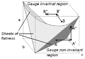
Figure 3: 3d color space of each vertex. All color-points inside the pyramid satisfy the conditions (1, 2). Point $A$ represents a flat vertex whose evolution kicks it out of the gauge invariant pyramid ($A^{\prime}$) and using a propagation rule can make it flat again. ($A^{\prime\prime}$)

The triangle inequalities (1) divide the 3d color space into two different regions. All gauge-invariant vertices are located inside or on the boundary of a pyramid bounded by three surfaces, which are given by the equations,

$$a+b=c,\ \ a+c=b,\ \ b+c=a;$$ (4)

where $a$, $b$ and $c$ are the colors of the three incident edges on a vertex. We call the three boundaries sheets of flatness. These correspond to flat triangles. We call the region a gauge invariant pyramid .

For a sandpile to be in a critical state, a fixed fraction of the steps between sites must be at the critical value such that the addition of one grain of sand will cause an avalanche of shifts of grains. The flat triangles play the same role in this model, they are the triangles whose next evolution, by the addition or subtraction of loops of flux, is likely to lead to gauge-non-invariant configurations. Hence in a critical state there must be a fixed fraction of such flat triangles. We will see that this expectation is satisfied when we find a set of rules that generates scale invariant distributions of avalanches.

In Borissov and Gupta’s model the vertices whose color-points are inside the gauge invariant pyramid (and are not flat) always are modified by the addition of positive colors. By adding a positive color to one of the edges of such a vertex, its color-point goes farther away from the origin of the color space. Roughly speaking, in this situation the probability of finding the new color-point on one of the sheets of flatness decreases. Therefore the probability of producing a flat vertex by a non-flat vertex is not high. In the simulation of the model it is clear that as time goes on, only small number of avalanches happen and for this reason the distribution of small size avalanches grows faster than larger ones. Thus the model does not exhibit a power law distribution of avalanches.

IV.2 Random vertex models

We now consider a different class of models, in which the evolution proceeds by adding or subtracting color simultaneously on all edges incident to a single vertex. We call these random vertex models.

The motivation for these models comes from looking at Figure 3. We see that if we subtract color from all three edges of a gauge invariant vertex (like $B$), the new point will be closer to one of the sheets of flatness. We then define a class of evolution rules based on choosing nodes rather than edges at random. In this class of rules, we will subtract the color $-2$ from all three edges incident on the chosen node.

The result can be to violate the gauge condition at that node and/or at adjacent nodes. To recover gauge invariance we need to define a propagation rule. One of the possible candidates is add +2 to all the three incident edges at the GNI-vertex. We call this simple rule the triangle propagation rule because it adds three equal colors to a trivalent vertex.

To specify the rule we have to give an ordering to the nodes. In our simulations, we use a simple ordering, left to right and top to bottom. We sweep the graph, checking the gauge invariance condition (1,2) at each node. When we find a GNI we act with the triangle propagation rule, by adding $+2$ to the colors on the edges incident to that node. When the checking is done once for all of the vertices, the sweep is repeated because new GNI-vertices may have been produced in the first sweep. We continue to repeat the propagation rule until all vertices become gauge invariant.

For example, consider the following network:

The first diagram shows a simple network. In the second step, it has been evolved by subtracting -2 from each edge incident to the vertex $c$. We then sweep the graph, from top to bottom and from left to right. Vertex $c$ remains gauge invariant but $b$ is not gauge invariant, so we act by adding $+2$ to each of its incident edges. But this makes $c$ a GNI-vertex. In the fourth step, +2 has been added to the edges incident to the vertex $c$. Doing so, this new network becomes gauge invariant. The number of steps in the avalanche in this evolution is $2$ because two vertices were updated in order to make the network gauge invariant.

Let’s summarize the random vertex class:

• Initialize the spin network by assigning random colors to its edges, requiring only that gauge invariance is satisfied at each node.

• Choose a vertex at random.

• Subtract a triangle of -2 from the three edges of the initial vertex.

• Check the gauge condition (1,2) at all vertices, by sweeping through the nodes according to some fixed rule. Fix each GNI-node by adding a triangle of +2 color to each edge of its dual triangle.

• Continue till the graph is again gauge invariant. Count the number of updated vertices. This is the size of the avalanche.

• Go back to the second step of the algorithm and repeat.

V Results

We now report on the simulation of the rule just described, which did lead to scale invariant behavior.

We did the simulation for a 2d planar spin network with 570 edges and 361 vertices. For the initial start we assigned random even numbers between 10 to 30 to each edge, requiring only that the graph be gauge invariant initially. Using the rules just described, we evolved the spin network labels for ten million steps. The result is shown in Figure 4.

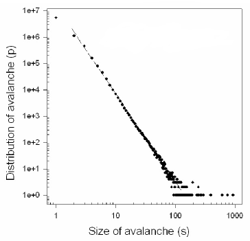
Figure 4: The log-log plot of the distribution of avalanche in a 2d planar spin network.

To completely define the evolution rule we mention:

• The nodes were always swept the same way, from left to right and up to down.

• It happens often that the color on an edge is reduced to $0$. The rules act on such edges as on the others, with the one exception that the $-2$ rule is never applied to a node when one of its edges is $0$, as that would lead to an edge with a negative color. However the triangle propagation rule acts on triangles with one or more edges zero as on other triangles. For example, a triangle with colors $(0,18,18)$ is gauge invariant, and so is skipped by the triangle propagation rule. But a triangle labelled $(0,2,4)$ is fixed, by adding $+2$ to each edge. The result is $(2,4,6)$, which is gauge invariant.

The distribution of the size of avalanches in a loglog scale behaves, to a good extent, linearly. Thus the dynamics of the triangle propagation rule on the spin network follows a power law and exhibits abelian self-organized critical behavior. The relation between the distribution of avalanche and the size of avalanche is:

$$P(s)=s^{-3.3}$$ (5)

to a good accuracy.

In a SOC model usually both area and size of avalanches are checked to behave power-law distributions. Area is the number of sites involved in an avalanche, no matter how many times they topple. In other word, the area is where the avalanche is taking place, and usually for larger lattices one finds larger areas, because it has a lattice dependent cut-off in its power-law distribution. If this distribution instead of being power-law is exponential, the avalanches do not expand in space and basically it does not matter if one takes a small or large lattice, as long as this is bigger than the maximum area that an exponential distribution is likely to give in finite samples marco .

To ensure this, we provide a typical plot of the distribution of area of avalanches. Figure 5 indicates the power-law behavior of area to a good accuracy in its distribution. Therefore, the macroscopic emerging of avalanches in space can be observed during this evolution of spin network. In other word, the avalanches do not resemble of some local resonances in a few nodes.

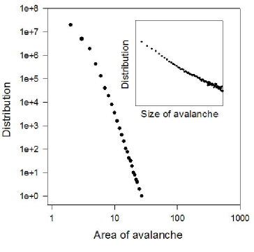
Figure 5: A typical log-log plot of the distribution of the area of avalanche and its corresponding log-log distribution of the size of avalanche.

In each time step of the evolution, we recorded the average of colors of the network and the fraction of the flat triangles, which are the cause of avalanche. In Figure 6 we see that the fraction of the number of flat vertices (or their dual triangles) is maintained about 0.3 during the simulation, while in Figure 7 we see how the average color in the spin network fluctuate in time.

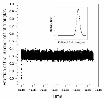
Figure 6: The fraction of flat triangles in time.

As color is proportional to length, Figure 7 exhibits a universe, described by our 2d planar spin network, expanding in time. The model, this is an example of self-organization not to an attractor state, but to an asymptote, on which the average radius has a constant rate of inflation (expansion), is critical, and exhibits avalanches of activity with power-law distributed sizes. This example demonstrates that self-organized critical behavior occurs in a larger class of systems than so far considered: systems not driven to an attractive fixed point, but, e.g., an asymptote, may also display self-organized criticality.

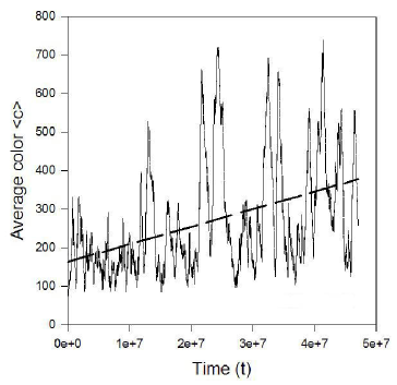
Figure 7: The average color of the spin network in time in fifty million iterations.

Finally, it is instructive to see how the evolution rule studied here affects the dual geometry, expressed in terms of the triangulation. In the Figure 8 we follow a piece of a dual spin network, as it evolves. We see the evolution is irregular in both time and space. Nevertheless, when averaged over large times and distances, a scale invariant behavior emerges.

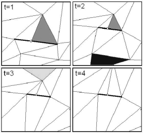
Figure 8: A few steps in the evolution of a part of a dual triangulation. The thick line (included a vertex in the middle) represents a flat triangle. At t=2, a triangle of color -2 is added to the shaded triangle, shrinking its sides. The triangle inequalities are violated on some neighboring triangles and these are resolved by addition of a triangle of color +2 to them. At t=3 we then iterate the procedure subtracting 2 from the edges of the black triangle and at t=4 we do the same to the bright gray one.

VI Conclusions

We have proposed a propagation rule for colors to evolve on a 2d planar open spin network, which appears to exhibit self-organized critical behavior.

It appears that with a special choice of evolution rule, the dynamics evolves the system to a dynamical equilibrium state, within which the behavior of the system appears to be scale invariant.

This work is a step in the investigation of the hypothesis that the emergence of our classical world from a discrete quantum geometry is analogous to a self-organized critical process. Among the further steps are 1) the study of models in which the underlying graphs themselves evolve by local rules, analogous to those studied here, 2) the study of other correlation functions, including those that would be interpreted as propagation amplitudes for matter and gravitational degrees of freedom, and 3) an increase in the valence, from three to four valent graphs, which is expected to correspond to the dynamics of geometry in $3+1$ dimensions, and 4) the demonstration that self-organized critical phenomena exists for quantum evolution and not just for ordinary statistical systems.

These are considerable challenges, towards which the present results must be seen as just a first step.

References

- (1) K. Wilson, The Renormalization Group: Critical Phenomena And The Kondo Problem, Journal-ref: Rev. Mod. Phys. 47 (1975) 773; K Wilson and J. Kogut, The Renormalization Group And Critical Phenomena, Rev. Mod. Phys. 55 (1983) 583.
- (2) C. Rovelli, Quantum Gravity. ISBN: 0521837332, Cambridge University Press; L. Smolin An invitation to loop quantum gravity, hep-th/0408048.
- (3) J. Ambjorn, J. Jurkiewicz and R. Loll, Phys. Rev. D64 (2001) 044011 [hep-th/0011276]; J. Ambjorn, J. Jurkiewiczcy and R. Loll, Emergence of a 4D World from Causal Quantum Gravity, hep-th/0404156. J. Ambjorn, Z. Burda, J. Jurkiewicz and C. F. Kristjansen, “Quantum gravity represented as dynamical triangulations,” Acta Phys. Polon. B 23, 991 (1992); J. Ambjorn, “Quantum Gravity Represented As Dynamical Triangulations,” Class. Quant. Grav. 12, 2079 (1995); M. E. Agishtein and A. A. Migdal, “Simulations of four-dimensional simplicial quantum gravity,” Mod. Phys. Lett. A 7, 1039 (1992).
- (4) Herbert W. Hamber, Ruth M. Williams, Non-Perturbative Gravity and the Spin of the Lattice Graviton , hep-th/0407039 and references contained therein.
- (5) P. Bak, C. Tang and K. Wiesenfeld, Phys. Rev. Lett. 59 (1987) 381; L. Pietronero, P. Tartaglia and Y. C. Zhang, Physica A 173 (1991) 22-44.
- (6) P. Bak, How Nature Works, Springer-Verlag, New York 1996.
- (7) D. L. Turcotte, Rep. Prog. Phys. 62 (1999) 1377-1429
- (8) F. Markopoulou and L. Smolin, Nucl. Phys. B508 (1997) 409
- (9) Fotini Markopoulou, “Dual formulation of spin network evolution”, gr-qc/9704013.
- (10) C. Rovelli, Phys. Rev. D48 (1993) 2702
- (11) J. Baez, Adv. Math. 117 (1996) 253-272 (gr-qc/941107); in “ The Interface of Knots and physics”, ed. L. Kauffman, A.M.S., Providence, (1996) 167-203
- (12) C. Rovelli and L. Smolin, Phys. Rev. D52 (1995) 5743-5759
- (13) R. Borissov and S. Gupta, Phys. Rev. D 60 (1999), 024002
- (14) J. W. Harris and H. Stocker, Handbook of Mathematics and Computational Science. New York: Springer-Verlag, 113, 1998.
- (15) M. Baiesi and C. Maes, cond-mat/0505274
- (16) M. Paczuski and P. Bak, (cond-mat/9906077)
- (17) B. A. Carreras, V. E. Lynch, D. E. Newman and R. Sanchez, Phys. Rev. E66 (2002) 011302
- (18) S. F. N rrelykke and P. BakPhys. Rev. E 65, 036147 (2002).
- (19) S. Boettcher and M. Paczuski, Phys. Rev. Lett. 79, 889-892 (1997).