Knot soliton in Weinberg-Salam model

Abstract

We study numerically the topological knot solution suggested recently in the Weinberg-Salam model. Applying the $SU(2)$ gauge invariant Abelian projection we demonstrate that the restricted part of the Weinberg-Salam Lagrangian containing the interaction of the neutral boson with the Higgs scalar can be reduced to the Ginzburg-Landau model with the hidden $SU(2)$ symmetry. The energy of the knot composed from the neutral boson and Higgs field has been evaluated by using the variational method with a modified Ward ansatz. The obtained numerical value is 39 Tev which provides the upper bound on the electroweak knot energy.

1. Introduction

It has been well known since 1980’s that knot-like topological solitons corresponding to a non-trivial Hopf number exist in some non-linear $\sigma$-models with a scalar field $n^{a},a=1,2,3$ vak ; vlad ; kundu . Last decade a wide class of such topological knot solitons have been proposed in various physical models: in the effective theory of quantum chromodynamics (QCD) fadd ; batt , in two-gap superconductivity models scond , and in two-component Bose-Einstein condensate theory bec ; batt2 ; chobec . Recently it was suggested that knot solitons could exist even in high energy physics, namely, in the Weinberg-Salam model chows .

In the present paper we consider numerically the properties of the knot soliton made of a neutral $Z$ boson with a dressing Higgs field in the Weinberg-Salam model. We apply the Ward ansatz ward which provided a high accuracy for the energy of the Faddeev-Niemi knot and results in, as we will show below, a reasonable value 39 Tev for the energy of the electroweak knot. Even though the obtained energy value seems to be out of practical detection with the present experimental facilities, the electroweak knot may have an impact on cosmological problems related to dark matter and baryon asymmetry of the universe rubak ; shap ; tur . In particular, it was suggested that the formation of primordial hypermagnetic knots and their further decay could result in the baryon asymmetry shap ; giov . We suppose that the existence of the topological knot in the standard model can lead to an alternative mechanism of the origin of the baryon asymmetry in the universe, like the baryogenesis scenario based on electroweak strings brand .

2. Gauge invariant Abelian projection

First we consider the $SU(2)$ Yang-Mills theory with a complex Higgs scalar doublet $\phi$ as a simple model of Weinberg-Salam theory. We will extract from the Lagrangian of the Weinberg-Salam model the part containing the interaction of the neutral boson with the Higgs scalar using the gauge invariant Abelian projection. By this way we keep explicitly the full $SU(2)$ gauge invariance and at the same time we preserve the topological structure of the original group $SU(2)$ in the Abelianized part of the gauge connection. This approach provides the gauge invariant definition of the Hopf number in terms of the Abelian potential and gives rise to the description of the neutral boson interacting with the Higgs scalar in the framework of a simple Ginzburg-Landau model.

We will follow the approach proposed in cho1 ; chows . Let us start from the gauge invariant Abelian projection which is given by the following decomposition of the full $SU(2)$ connection cho1

$$\vec{A}_{\mu}=A_{\mu}\hat{n}-\displaystyle\frac{1}{g}\hat{n}\times\partial_{\mu}\hat{n}+{\vec{W}}_{\mu}=\hat{A}_{\mu}+{\vec{W}}_{\mu},$$

$$(A_{\mu}=\hat{n}\cdot\vec{A}_{\mu},~{}\hat{n}^{2}=1,~{}\hat{n}\cdot\vec{W}_{\mu}=0).$$ (1)

The restricted potential $\hat{A}_{\mu}$ possesses transformation properties of the full $SU(2)$ connection and leads to the desired Abelianization of the theory. The vector part of the restricted potential $\vec{C}_{\mu}\equiv-\displaystyle\frac{1}{g}\hat{n}\times\partial_{\mu}\hat{n}$ is defined in terms of the triplet scalar field $\hat{n}$ whose configuration is classified by Hopf invariant, i.e. by a homotopy group $\pi_{3}(S^{2})$. The scalar field $\hat{n}$ is covariantly constant

$${\hat{D}}_{\mu}\hat{n}=\partial_{\mu}\hat{n}+g{\hat{A}}_{\mu}\times\hat{n}=0$$ (2)

and represents the topological degrees of freedom in the theory. The $SU(2)$ gauge transformations can be written as follows

$$\delta\hat{n}=-\vec{\alpha}\times\hat{n}\,,\,\,\,\,\delta{\vec{A}}_{\mu}=\displaystyle\frac{1}{g}D_{\mu}\vec{\alpha},$$ (3)

or

$$\delta A_{\mu}=\displaystyle\frac{1}{g}\hat{n}\cdot\partial_{\mu}{\vec{\alpha}},\,\,\,\ \delta\hat{A}_{\mu}=\displaystyle\frac{1}{g}{\hat{D}}_{\mu}{\vec{\alpha}},$$

$$\hskip 34.14322pt\delta{\vec{W}}_{\mu}=-{\vec{\alpha}}\times{\vec{W}}_{\mu}.$$ (4)

In a local orthonormal frame $(\hat{n}_{1},\hat{n}_{2},\hat{n}_{3}\equiv\hat{n})$ of the internal $SU(2)$ space one can rewrite the decomposition (Knot soliton in Weinberg-Salam model) as

$$\vec{A}_{\mu}=A_{\mu}\hat{n}+(\omega_{\mu}^{(1,2)}+{\vec{W}}_{\mu}^{(1,2)})\hat{n}_{(1,2)},$$ (5)

where $\omega_{\mu}^{(1,2)},\,{\vec{W}}_{\mu}^{(1,2)}$ are local components of the vectors ${\vec{C}}_{\mu},{\vec{W}}_{\mu}$ correspondingly. By appropriate gauge transformation one can pass to the magnetic gauge cho1 in which the vector potential $\vec{C}_{\mu}$ converts into the Abelian magnetic potential $C_{\mu}$

$$\vec{A}_{\mu}=(A_{\mu}+C_{\mu})\hat{n}+{\vec{W}}_{\mu},$$

$$C_{\mu}=-\displaystyle\frac{1}{g}\hat{n}_{1}\partial_{\mu}\hat{n}_{2}.$$ (6)

With the decomposition (Knot soliton in Weinberg-Salam model) one can factorize the Abelian potential part and the off-diagonal components in an explicit gauge invariant manner

$$\vec{F}_{\mu\nu} = (F_{\mu\nu}+H_{\mu\nu})\hat{n}$$ (7)

$$+{\hat{D}}_{\mu}{\vec{W}}_{\nu}-{\hat{D}}_{\nu}{\vec{W}}_{\mu}+g{\vec{W}}_{\mu}\times{\vec{W}}_{\nu},$$

where

$$F_{\mu\nu}=\partial_{\mu}A_{\nu}-\partial_{\nu}A_{\mu},$$

$$H_{\mu\nu}=-\displaystyle\frac{1}{g}\epsilon^{abc}\hat{n}^{a}\partial_{\mu}\hat{n}^{b}\partial_{\nu}\hat{n}^{c}=\partial_{\mu}C_{\nu}-\partial_{\nu}C_{\mu}.$$ (8)

So that the Lagrangian can be rewritten in the form

$${\cal L}=-\displaystyle\frac{1}{4}\vec{F}^{2}_{\mu\nu}$$

$$=-\displaystyle\frac{1}{4}(F_{\mu\nu}+H_{\mu\nu})^{2}-\displaystyle\frac{1}{4}({\hat{D}}_{\mu}{\vec{W}}_{\nu}-{\hat{D}}_{\nu}{\vec{W}}_{\mu})^{2}-$$

$$\displaystyle\frac{g}{2}(F_{\mu\nu}+H_{\mu\nu})\cdot({\vec{W}}_{\mu}\times{\vec{W}}_{\nu})-\displaystyle\frac{g^{2}}{4}({\vec{W}}_{\mu}\times{\vec{W}}_{\nu})^{2}.$$ (9)

In complex notation for the charged vector boson

$$W_{\mu}=\displaystyle\frac{1}{\sqrt{2}}(W^{1}_{\mu}+iW^{2}_{\mu}),$$ (10)

one can express the Lagrangian explicitly in terms of the Abelian potential $A_{\mu}+C_{\mu}$ and the charged vector field $W_{\mu}$,

$${\cal L}=-\displaystyle\frac{1}{4}(F_{\mu\nu}+H_{\mu\nu})^{2}-\displaystyle\frac{1}{2}|{D}_{\mu}{W}_{\nu}-{D}_{\nu}{W}_{\mu}|^{2}$$

$$+ig(F_{\mu\nu}+H_{\mu\nu})\stackrel{{\scriptstyle\ast}}{{W}}_{\mu}W_{\nu}-\displaystyle\frac{g^{2}}{2}\Big{[}(\stackrel{{\scriptstyle\ast}}{{W}}_{\mu}W_{\mu})^{2}$$

$$-(\stackrel{{\scriptstyle\ast}}{{W}}_{\mu})^{2}(W_{\nu})^{2}\Big{]}=-\displaystyle\frac{1}{4}(F_{\mu\nu}+H_{\mu\nu}+W_{\mu\nu})^{2}$$

$$-\displaystyle\frac{1}{2}|{D}_{\mu}{W}_{\nu}-{D}_{\nu}{W}_{\mu}|^{2},$$ (11)

where

$$W_{\mu\nu}=-ig(\stackrel{{\scriptstyle\ast}}{{W}}_{\mu}W_{\nu}-\stackrel{{\scriptstyle\ast}}{{W}}_{\nu}W_{\mu}),$$

$${D}_{\mu}{W}_{\nu}=(\partial_{\mu}+ig(A_{\mu}+C_{\mu}))W_{\nu}.$$

It should be stressed, that the Lagrangian is invariant not only under the original $SU(2)$ group transformations but under the action of the dual $\tilde{U}(1)$ group as well

$$\delta_{SU(2)}(A_{\mu}+C_{\mu})=0,$$

$$\delta_{\tilde{U}(1)}(A_{\mu}+C_{\mu})=\partial_{\mu}\tilde{\lambda}.$$ (12)

Due to this the Hopf number can be defined as a Chern-Simons index of $SU(2)$ gauge theory. For the case $A_{\mu}=0$ employed later on we have the standard formula for the Hopf number cho1

$$N_{H}=\displaystyle\frac{g^{2}}{32\pi^{2}}\int d^{3}x\epsilon_{ijk}C_{i}H_{jk}.$$ (13)

Notice, the Abelian symmetry ${\tilde{U}}(1)$ has been appeared in QCD as a dual magnetic symmetry cho1 which is an essential ingredient of the dual Meissner effect leading to the monopole mechanism of confinement.

With these preliminaries let us start from the bosonic sector of the Weinberg-Salam Lagrangian

$${\cal L}=-\displaystyle\frac{1}{4}({\vec{F}}_{\mu\nu})^{2}-\displaystyle\frac{1}{4}(G_{\mu\nu})^{2}-|(\partial_{\mu}-\displaystyle\frac{ig}{2}\vec{\sigma}\cdot\vec{A}_{\mu}$$

$$-ig^{\prime}B_{\mu}){\tilde{\phi}}|^{2}-\displaystyle\frac{\lambda}{2}({\tilde{\phi}}^{\dagger}{\tilde{\phi}}-\displaystyle\frac{v^{2}}{2})^{2},$$

$$G_{\mu\nu}=\partial_{\mu}B_{\nu}-\partial_{\nu}B_{\mu},$$ (14)

where $B_{\mu}$ is the Abelian potential corresponding to the weak hypercharge group $U_{Y}(1)$.

We consider the restricted case with the vanishing charged vector boson $W_{\mu}=0$ and electromagnetic field $A_{\mu}=0$ while keeping only the Higgs field ${\tilde{\phi}}$ and the neutral $Z$ boson in the Lagrangian. We will identify the classical part of $Z$ boson containing the whole topological content of the knot with a hypermagnetic potential $C_{\mu}$ chows . It is convenient to express the fields $\hat{n},{\tilde{\phi}}$ in terms of the real components $\rho,\alpha$ and $SU(2)$ complex doublet $\xi$ which parametrizes the complex projective space $CP^{1}$

$$\hat{n}^{a}=\xi^{+}{\vec{\sigma}}^{a}\xi,$$

$${\tilde{\phi}}=\displaystyle\frac{1}{\sqrt{2}}\xi\rho e^{i\alpha}\equiv\displaystyle\frac{1}{\sqrt{2}}\xi\phi,$$

$$\xi^{+}\xi=1.$$ (15)

Since the hypermagnetic potential $C_{\mu}$ is the dual potential one can express it locally as follows

$$C_{\mu}=\displaystyle\frac{4i}{\bar{g}}\xi^{+}\partial_{\mu}\xi.$$ (16)

With this we obtain the final expression for the Lagrangian for our purpose to study the static knot type solution

$${\cal L}=-\displaystyle\frac{1}{4}H_{\mu\nu}^{2}-|(\partial_{\mu}+i\displaystyle\frac{\bar{g}}{2}C_{\mu})\phi|^{2}-\displaystyle\frac{\lambda}{2}(|\phi|^{2}-\rho_{0}^{2})^{2}.$$

(17)

Formally, the expression (17) can be easily recognized as a well-known Ginsburg-Landau Lagrangian. But one should stress that the original non-Abelian structure of the Lagrangian (17) is hidden and encoded in the topological properties of the hypermagnetic potential $C_{\mu}$ given by (16). By this the non-trivial homotopy group $\pi_{3}(CP^{1})$ ensures the existence of the topological knot solution classified by Hopf number $N_{H}$.

3. Knot soliton

The idea of a non-topological string in the electroweak theory was proposed long time ago nambu . Later the twisted electroweak strings with a baryon number had been introduced in vach , and the existence of the knot in the Weinberg-Salam model was suggested recently chows . We will find the static topological knot solution by minimization of the energy functional corresponding to the Lagrangian (17) ($i=1,2,3$)

$$E=\int d^{3}x{\cal E}=\int d^{3}x\Big{[}\displaystyle\frac{1}{4}H_{ij}^{2}+\displaystyle\frac{1}{2}(\partial\rho)^{2}$$

$$+\displaystyle\frac{{\bar{g}}^{2}}{8}\rho^{2}(C_{i}+\frac{2}{\bar{g}}\partial_{i}\alpha)^{2}+\displaystyle\frac{\lambda}{8}(\rho^{2}-v^{2})^{2}\Big{]}.$$ (18)

Let us introduce the dimensionless variables $r\rightarrow rm_{W},\,\,k\equiv 2\sqrt{\lambda}/g=m_{H}/m_{W},\,\,C_{i}\rightarrow C_{i}g/m_{W},\,\,\rho\rightarrow\rho/v$ with rescaling $\alpha\rightarrow\alpha\cos\theta_{W}$ and $m_{W}=80.22$ Gev , $m_{H}=200$ Gev, $\,\sin^{2}\theta_{W}=0.2325$. One can rewrite the energy functional in terms of the dimensionless variables as follows

$$E=\displaystyle\frac{m_{W}}{g^{2}}\int d^{3}x\Big{[}\displaystyle\frac{1}{2}{\vec{H}}^{2}+2(\partial\rho)^{2}$$

$$+\displaystyle\frac{1}{2\cos^{2}\theta_{W}}\rho^{2}(C_{i}+2\partial_{i}\alpha)^{2}+\displaystyle\frac{k^{2}}{2}(\rho^{2}-1)^{2}\Big{]},$$ (19)

where $(\vec{H})_{i}=\epsilon_{ijk}\partial_{j}C_{k}$ is the hypermagnetic field strength of the neutral boson.

To find out appropriate trial functions we start from the original Ward ansatz ward . The stereographic projection of $\hat{n}$ is given by a complex field

$$Z=\displaystyle\frac{n_{1}+in_{2}}{1+n_{3}}.$$ (20)

The Ward ansatz ward with a radial trial function $f(r)$

$$Z=\displaystyle\frac{x+iy}{z-if(r)},$$

$$f(r)=a(r-b)(r^{2}+cr+d)$$ (21)

was proposed to describe the Faddeev-Niemi knot soliton with a good accuracy for the energy value. The non-trivial Hopf number $N_{H}=1$ is determined by the boundary conditions of the function $f(r)$ at points $r=0,\,\infty$. Applying this ansatz with the trial function $f(r)$ and the definitions (15) one can find the corresponding expression for the complex doublet $\xi$ (in spherical coordinates)

$$\xi=\left(\begin{array}[]{c}\sqrt{\frac{h^{2}(r)+\cos^{2}\theta}{1+h^{2}(r)}}\\ \frac{\sin\theta}{\sqrt{1+h^{2}(r)}}e^{i\psi(r,\theta,\varphi)}\end{array}\right),$$ (24)

$$\tan\psi(r,\theta,\varphi)=\frac{\sin\varphi\cos\theta+h(r)\cos\varphi}{\cos\varphi\cos\theta-h(r)\sin\varphi},$$ (25)

where $h(r)=f(r)/r$. With this one can write down the components of the magnetic potential

$$C_{r} = \displaystyle\frac{2h^{\prime}\sin^{2}\theta\cos\theta}{(1+h^{2})(h^{2}+\cos^{2}\theta)},$$

$$C_{\theta} = \displaystyle\frac{2h\sin^{3}\theta}{r(1+h^{2})(h^{2}+\cos^{2}\theta)},$$

$$C_{\varphi} = \displaystyle\frac{2\sin\theta}{r(1+h^{2})}.$$ (26)

One can use the gauge freedom to remove the dependence of the phase factor $\psi(r,\theta,\varphi)$ on the variables $(r,\theta)$. By making an appropriate gauge transformation

$$C_{i}\rightarrow C_{i}-2\nabla_{i}\arctan(\frac{h}{\cos\theta}),$$

$$\psi(r,\theta,\varphi)\rightarrow\psi(r,\theta,\varphi)-\arctan(\frac{h}{\cos\theta})$$ (27)

one results in a simple parametrization for the phase factor $\psi(r,\theta,\varphi)=\varphi$ and for the components $C_{r},C_{\theta}$

$$C_{r}=-\frac{2h^{\prime}\cos\theta}{1+h^{2}},$$

$$C_{\theta}=-\frac{2h\sin\theta}{r(1+h^{2})}.$$ (28)

The phase factor in the scalar field $\phi=\rho e^{i\alpha}$ appears in the Lagrangian only in the combination $C_{i}+2\partial_{i}\alpha$. We will adopt the following ansatz for the phase factor $\alpha(r,\theta)=\beta(r)\cos\theta$ with the boundary conditions $\beta(0)=\beta(\infty)=0$. The chosen form of the ansatz preserves the Hopf number calculated with the gauge transformed potentials

$$C_{r}=-\frac{2h^{\prime}\cos\theta}{1+h^{2}}+2\beta^{\prime}(r)\cos\theta,$$

$$C_{\theta}=-\frac{2h\sin\theta}{r(1+h^{2})}-\displaystyle\frac{2\beta(r)}{r}\sin\theta,$$

$$C_{\varphi}=\frac{2\sin\theta}{r(1+h^{2})}.$$ (29)

It turns out that the modified ansatz (29) provides lower value of the minimum of the energy functional. For the Higgs field $\rho(r,\theta)$ we impose the boundary conditions

$$\rho(0,\theta)=c,\,\,\,\,\rho(\infty,\theta)=1,$$ (30)

where $c$ is a number. The minimization of the energy functional gives the energy of the knot $E_{0}=39$ Tev. This energy value has been checked with a class of various trial functions including the angle dependence on $\theta$. We found that the minimum of the energy functional is reached for a spherically symmetric configuration of the Higgs field. We expect that our modified Ward ansatz (29) with a pure radial trial function for the Higgs field $\rho(r)$ provides the main contribution to the knot energy similar to the case of the Faddeev-Niemi knot. The energy density plots in the plane $XY$ and $XZ$ are shown in Figs. 1, 2 from which one can see that the energy of the knot is localized along the torus.

The topological stability of the knot is provided by non-vanishing hypermagnetic fluxes along and around the torus. The total hypermagnetic flux around the axis $0Z$ is $\Phi_{\varphi}=2\pi$. The total hypermagnetic flux through the inner disk of the torus ($r<r_{0}=1.64,\theta=\pi/2$) is $\Phi_{z}=2\pi$. By this we have the linking of two fluxes which provides the Hopf number $Q_{H}=1$ and the topological stability. Notice, that the lines of the hypermagnetic vector field $\vec{H}$ form in fact a twisted torus.

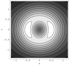
Figure 1: The contour plot of the energy density of the knot in the plane $y=0$. The maximal value of the energy density is ${\cal E}_{max}=7.42$ , the step size between the contours is $0.39$ (in units of $v/g=0.407$ Tev/$m^{3}$).

One should stress, since we use a variational method with a constrained ansatz we can not rather obtain a more detailed structure of the energy density distribution of the knot. By plotting the energy density one can describe only qualitatively the inner structure of the knot and estimate roughly the effective size of the knot. The energy density has a maximum along the circle $r_{0}=0.50,\theta=\pi/2$ which corresponds to the radius of the knot $1.45\times 10^{-18}m$. From the other hand we can define the radial size of the knot as a radius of the circle at which the hypermagnetic component $H_{\theta}$ changes its sign. This gives the radius $r_{0}=4.1\times 10^{-18}m$ which is near the value $3.5\times 10^{-18}m$ estimated in chows . Notice, that the Ward ansatz gives exactly the Dirac type magnetic flux quantization with the minimal non-zero flux $\Phi=2\pi$ due to the semi-simple structure of the electroweak gauge group $SU(2)\times U_{Y}(1)$ and the non-compactness of the electric charge group $U_{e}(1)$.

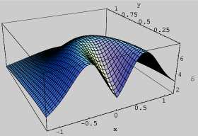
Figure 2: The energy density ${\cal E}(x,y,0)$ of the knot in the plane $z=0$

For a model with a simple gauge group $SU(2)$ we would have Wu-Yang type flux quantization with a flux quantum proportional to $4\pi$. Such situation has been realized, for instance, in a two-component Bose-Einstein condensate system chobec . The energy density and hypermagnetic field components $H_{\theta},H_{\varphi}$ in the plane $\theta=\pi/2$, the Higgs field $\rho(r)$ and the phase radial function $\beta(r)$ are shown in Fig. 3.

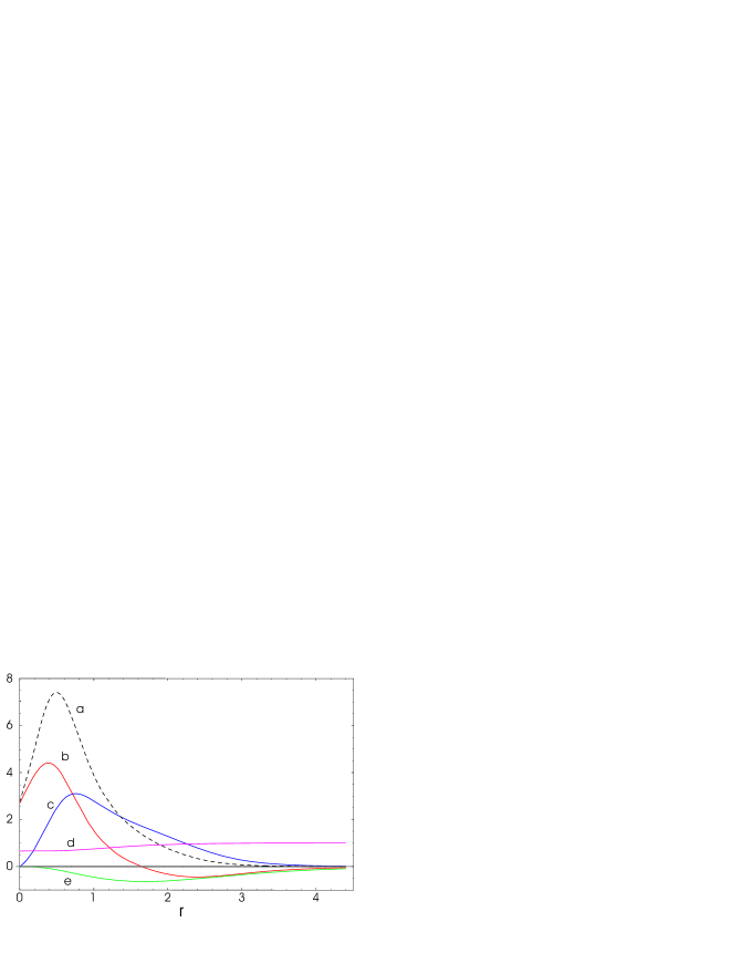
Figure 3: (a) the energy density ${\cal E}(r,\pi/2)$ (in unit of $v/g$); (b) the hypermagnetic field $H_{\theta}(r,\pi/2)$; (c) the hypermagnetic field $H_{\varphi}(r,\pi/2)$, (d) the Higgs field $\rho(r)$; (e) the phase radial function $\beta(r)$ (in dimensionless units).

Since the energy of the knot is much greater than the energy of vector $W,Z$ bosons an important question arises whether the knot solution is stable against the interaction with other fields, especially with the charged $W$ boson and electromagnetic field. The only potentially dangerous part in the Weinberg-Salam Lagrangian which can cause the instability is represented by the so called anomalous magnetic moment interaction term $igH_{\mu\nu}\stackrel{{\scriptstyle\ast}}{{W}}_{\mu}W_{\nu}$ in (Knot soliton in Weinberg-Salam model). This term leads to a severe vacuum instability problem in QCD via generating a tachyonic mode niel .

To analyse the stability of the knot soliton we consider small fluctuations of $W$ field in knot background. The possible unstable modes are determined by the negative eigenvalues of the operator $K$ defined by means of the second variational derivative of the Lagrangian with respect to infinitesimal variations $\delta W_{\mu}$. In a suitable background gauge $(\partial_{\mu}+ig\cos\theta_{W}C_{\mu})W_{\mu}=0$ one can find the operator $K$ as follows (in dimensionless variables)

$$K_{\mu\nu}=-\displaystyle\frac{m_{W}}{g^{2}}\Big{[}\eta_{\mu\nu}(D_{\rho}D_{\rho}-\rho^{2})+i\frac{e}{g^{\prime}}Z_{\mu\nu}\Big{]},$$

$$Z_{\mu\nu}=\partial_{\mu}C_{\nu}-\partial_{\nu}C_{\mu},$$ (31)

where, $D_{\mu}=\partial_{\mu}+i\frac{e}{g^{\prime}}C_{\mu}$. One can factorize the eigenvalues of the matrix part with Lorentzian indices in the operator $K$ similarly to the case of derivation of functional determinants corresponding to the one-loop effective action in $SU(2)$ QCD (details of derivation for general magnetic and electric background are given in choqcd )

$$K^{\pm}\simeq-D_{i}D_{i}+\rho^{2}\pm 2\frac{e}{g^{\prime}}H,$$ (32)

where $H\equiv|\vec{H}|$. With $C_{\mu}$ defined by (29) one can write down the eigenfunction equation for the operator $K^{\pm}$

$$\Big{[}-\displaystyle\frac{1}{r^{2}}\partial_{r}(r^{2}\partial_{r})-\displaystyle\frac{1}{r^{2}\sin\theta}\partial_{\theta}(\sin\theta\partial_{\theta})-\frac{2ie}{g^{\prime}}C_{i}\partial_{i}-$$

$$\frac{ie}{g^{\prime}}\partial_{i}C_{i}+\frac{e^{2}}{g^{\prime 2}}C_{i}^{2}+\rho^{2}\pm\frac{2e}{g^{\prime}}H\Big{]}\Psi(r,\theta)=\Lambda\Psi(r,\theta)$$ (33)

The equation represents a Schrodinger type problem for a quantum mechanical particle moving in a potential well. To estimate the lowest eigenvalue corresponding to the ground state one can neglect the terms $2iC_{i}\partial_{i}$ and $i\partial_{i}C_{i}$ which do not contribute to the ground state in the leading order approximation due to the axial symmetry and linear dependency of the knot solution $C_{i}$ on angle functions. The negative eigenvalues can arise only from the equation with the lower negative sign in front of the last term in l.h.s of (33). With this, substituting the numerical knot solution into the equation and solving it by the variational method one can find the lowest eigenvalue which is found to be a positive number $\Lambda_{0}=+0.31\,$. The scalar field $\rho$ plays a role of the mass regulator parameter which is close to the mass of $W$ boson (see Fig.3). One can find numerically that negative modes would appear if $\rho$ were replaced with a constant averaged value less than $0.73$. Surprisingly, despite on the facts that the knot energy is much higher than the energy of $W$ boson, and our solution is obtained with a simple modified Ward ansatz, nevertheless, no any negative eigenvalues appear. The weak dependency on the knot energy is provided by the presence of two competetive terms in (33), $\displaystyle\frac{e^{2}}{g^{\prime 2}}C_{i}^{2}$ and $-\displaystyle\frac{2e}{g^{\prime}}H$, which contribute opposite ways to the quantum mechanical potential in the Schrodinger equation. We have checked also that unstable modes do not appear under small deviation of the profile functions $f,\rho,\alpha$ from the numerical solution. This analysis gives us a hope that a rigorous exact solution for the knot will be stable as well.

In conclusion, we performed numerical study of the topological knot soliton in the Weinberg-Salam model suggested in chows . The obtained numerical value of the knot energy is 39 Tev which is higher than the earlier estimate 21 Tev chows . The last estimate was based on the equation for the knot energy obtained in the non-linear $\sigma$-model vak which represents actually the low energy bound. Since we elaborate the energy of the knot with the variational method, our numerical result provides the upper bound which, we believe, is close to the real value for the energy of the electroweak knot. The knot energy value even being much higher than the scale $100$ Gev of the standard model, it is still less than the scale of the temperature $T\simeq 80$ Tev for the right-electron equilibration state considered in estimation of the baryon asymmetry camp ; oliv . This might be an indication that the topological electroweak knot could play an important role in cosmology at the stage of formation of large scale structures along with other proposed mechanisms.

Acknowledgements

One of authors (D.G.P.) thanks Y. M. Cho for useful discussions and helpful comments. This work was partially supported by INTAS grant 2000-110.

References

- (1) A. F. Vakulenko and L. V. Kapitanski, Dokl. Acad. Nauk USSR 246 (1979) 840.
- (2) Vladimirov S. A., Teor. Mat. Fisika (Sov. Phys. J.) 44 (1980) 410.
- (3) Kundu A. and Rubakov Yu. P., J. Phys., A15 (1982) 269.
- (4) L. Faddeev and A. Niemi, Nature 387 (1997) 58.
- (5) R. Battye and P. Sutcliffe, Phys. Rev. Lett. 81 (1998) 4798.
- (6) E. Babaev, Phys. Rev. Lett. 88 (2002) 177002; E. Babaev, L. Faddeev, and A. Niemi, Phys. Rev. B65 (2002) 100512; Y. M. Cho, cond-mat/0112498.
- (7) J. Ruostekoski and J. Anglin, Phys. Rev. Lett. 86 (2001) 3934; H. T. C. Stoof, E. Vliegen, U. Al Khawaja, Phys. Rev. Lett. 87 (2001) 120407;
- (8) R. Battye, N. Cooper, and P. Sutcliffe, Phys. Rev. Lett. 88 (2002) 080401; C. Savage and J. Ruostekoski, Phys. Rev. Lett. 91 (2003) 010403.
- (9) Y. M. Cho, cond-mat/0409636.
- (10) Y. M. Cho, hep-th/0110076.
- (11) R. S. Ward, Phys. Lett. B473 (2000) 291.
- (12) V. Rubakov, Prog. Theor. Phys. 75 (1986) 366;A. N. Redlich and L. C. R. Wijewardhana, Phys. Rev. Let. 54 (1984) 970.
- (13) M. E. Shaposhnikov, JETP Lett. 44 (1986) 465;Nucl. Phys. B 287 (1987) 757; ibid 299 (1988) 797.
- (14) N. Turok, in: Perspectives on Higgs Physics, ed. by G. Kane (World Sci., Singapore, 1992) p. 300; A. G. Cohen, D. B. Caplan and A. E. Nelson, Ann. Rev. Nucl. Part. Sci. 43 (1993) 27.
- (15) M. Giovannini, Phys. Rev. D61 (2000) 063502; 063004 (ibid).
- (16) R. Brandenberger and A. C. Davis, Phys. Lett. B308 (1993) 79.
- (17) Y. M. Cho, Phys. Rev. D21 (1980) 1080; Phys. Rev. Lett. 46 (1981) 302; Phys. Rev. D23 (1981) 2415.
- (18) Y. Nambu, Nucl. Phys. B130 (1977) 505.
- (19) T. Vachaspati and G. B. Field, Phys. Rev. Lett. 73 (1994) 373.
- (20) N. K. Nielsen and P. Olesen, Nucl. Phys. B160, 380 (1979); C. Rajiadakos, Phys. Lett. B100, 471 (1981).
- (21) Y. M. Cho and D. G. Pak, Phys. Rev. D65, 074027 (2002).
- (22) B. Campbell, S. Davidson, J. Ellis and K. Olive, Phys. Lett. 297B (1992) 118; L. E. Ibanez and F. Quevedo, Phys. Lett., B283 (1992) 261.
- (23) J. M. Cline, K Kainulainen and K. A. Olive, Phys. Rev. Lett. 71 (1993) 2372; Phys. Rev. D 49 (1993) 6394.