The Casimir Energy for a Hyperboloid Facing a Plate in the Optical Approximation

Abstract

We study the Casimir energy of a massless scalar field that obeys Dirichlet boundary conditions on a hyperboloid facing a plate. We use the optical approximation including the first six reflections and compare the results with the predictions of the proximity force approximation and the semi-classical method. We also consider finite size effects by contrasting the infinite with a finite plate. We find sizable and qualitative differences between the new optical method and the more traditional approaches.

I Introduction

The last ten years have seen a revolution in experimental techniques used to measure the Casimir effect Casimir ; expt1 ; MPnew . These new techniques open the door to measurements at a precision where interesting geometrical dependence can be expected MPnew . However no exact calculations are available for geometries other than parallel plates. Traditionally the only tool for estimating Casimir energies for other geometries has been the proximity force approximation (PFA), which treats all geometries as superpositions of infinitesimal parallel plates Derjagin , a crude approximation.

It is therefore interesting to develop approximations that might provide an accurate estimate of the Casimir energy for other, experimentally relevant geometries. Recently we have developed a new, approximate treatment of Casimir effects for sufficiently smooth but otherwise arbitrary geometries based on geometric optics pap1 ; opt1 . We have tested the optical method by comparing with a precise numerical calculation Gies03 for the case of a sphere facing a plate. The optical approximation agrees much better with the numerical results than does the PFA. So far, it has not been possible to provide a useful estimate of the corrections to the optical approximation, which involve diffractive contributions.

Some years ago Schaden and Spruch proposed a“semi-classical” approximation based on Gutzwiller’s approximation for the density of states SandS ; Gutz . This approximation treats high frequency effects correctly and is exact for planar surfaces. It also captures important effects of curvature, which are clearly omitted in the PFA. However, as we will see, it does not seem to capture other important aspects of the geometry. For example, it is sensitive only to the curvature of the boundaries at their points of closest approach, whereas the general form of the problem suggests much more complex dependence on the geometry.

In this paper we apply the optical approach to the study of the experimentally relevant example of a hyperboloid facing a plate. We consider a scalar field and impose Dirichlet boundary conditions. We are interested in the force between the hyperboloid and the plate, or equivalently, the interaction energy, from which divergent self-energies that do not contribute to the force have been subtracted. This problem has no closed, analytic solution, nor has it been studied with the numerical methods of Gies et al. Gies03 but it seems like a good candidate for future experimental studies. We find that the optical estimate of the Casimir energy differs significantly from the other approximations especially when the opening angle of the hyperboloid is small.

The optical method can be applied also when the bounding surfaces are finite, so in order to assess the effects of finiteness we study the configuration of a hyperboloid opposite to a finite plate. We find and explain differences between the optical approach on the one hand and the PFA and the semi-classical approach of Ref. SandS on the other. This application illustrates the shortcomings of the semi-classical approximation and the more subtle difference between the PFA and the optical approximation. In particular it helps clarify in which sense the optical approximation is a uniform semi-classical approximation.

The broad interest in Casimir physics and the application of new experimental methods will certainly allow tests which can distinguish among these different approaches, and guide theory toward a correct treatment of the dependence of Casimir effects on geometry.

II The Optical Approach to Casimir Energies

We want to calculate the Casimir energy of a quantized scalar field obeying boundary conditions on the border $\partial{\cal D}$ of the domain ${\cal D}$ limited by impenetrable bodies. This is an idealization of a physical interaction that prevents the field from entering the bodies. In the case of physical interest the electromagnetic field interacts with the electrons in metallic bodies. The interactions can be idealized by conducting boundary conditions for momenta $k\ll\Lambda$ where $\Lambda$ is a cutoff. For the case of the metal and electromagnetic field, the cutoff is of order of the plasma frequency of the material. The Casimir energy depends on $\Lambda$, and would diverge if $\Lambda$ were taken to infinity. So the cutoff cannot be removed in the fashion familiar from renormalizable quantum field theories. This is not a problem for us, however. First, the would-be divergences are associated with the self-energies of the bodies and do not contribute to forces (or interaction energies) between rigid bodies Graham:2003ib , which are what concerns us here. Second, finite cutoff dependence can be ignored when the minimum distance between the two bodies, $h$, is much larger than the inverse cutoff, i.e. $h\gg 1/\Lambda$ pap1 ; opt1 .

The Casimir energy for a massless scalar field $\phi$ living inside the domain ${\cal D}\subset\mathbb{R}^{3}$ with Dirichlet boundary conditions on the surface $\partial{\cal D}$ can be written as Graham:2002xq

$${\cal E}_{{\cal D}}[\phi]=\frac{1}{2}\hbar\ \int_{0}^{\infty}dk\int_{{\cal D}}d^{3}x\ \omega(k)\rho(x,k),$$ (1)

where in the case of massless fields $\omega(k)=ck$, and the (local) density of states $\rho(x,k)$ is related to the propagator $G(x^{\prime},x,k)$ of the Helmholtz equation by

$$\rho(x,k)=\frac{2k}{\pi}\ {\rm Im}\ G(x,x,k),$$ (2)

and the standard density of states is $\rho(k)=\int d^{3}x\ \rho(x,k)$. The equation satisfied by $G$ is

$$(-\Delta^{\prime}-k^{2})G(x^{\prime},x,k) = \delta^{3}(x^{\prime}-x)\ \mbox{if}\ x,x^{\prime}\in{\cal D}$$

$$G(x^{\prime},x,k) = 0\ \mbox{if }x^{\prime}\mbox{ or }x\in\partial{\cal D}.$$ (3)

The essence of the optical approximation is to replace the Helmholtz propagator, eq. (II), with an approximation taken from wave optics pap1 ; opt1 which assumes that the path integral representation for $G(x,x^{\prime},k)$ is saturated by its stationary points, i.e. straight line paths making specular reflections (accompanied by a phase change) at the boundaries. In this way the intractable sum over modes is replaced by a tractable, but approximate sum over paths,

$${\cal E}_{\rm optical}=-\frac{\hbar c}{2\pi^{2}}\sum_{\bf n}(-1)^{n}M_{n}\int_{{\cal D}_{\bf n}}d^{3}x\frac{\sqrt{\Delta_{\bf n}(x)}}{\ell_{\bf n}^{3}(x)}\,.$$ (4)

Here the sum runs over the optical paths indexed by ${\bf n}$ (which is an index taking care of both the number of reflections $n$ and the sequence of bodies on which the reflections occur), $\ell_{\bf n}(x)$ is the length of the closed path starting and ending at $x$ and ${\cal D}_{{\bf n}}$ is its domain of existence (which can be smaller than ${\cal D}$), $M_{n}$ is the multiplicity of the path ${\bf n}$ ($M_{n}=1$ for paths with an odd number of reflections, $M_{n}=2$ for paths with an even number of reflections) and $\Delta_{\bf n}(x)$ is shorthand for the enlargement factor $\Delta_{\bf n}(x,x)$:

$$\Delta_{\bf n}(x^{\prime},x)=\frac{d\Omega_{x}}{dA_{x^{\prime}}}$$ (5)

is the ratio between the angular opening of an arbitrarily narrow pencil of rays following the optical path ${\bf n}$ starting at the initial point $x$ and the area spanned at the final point $x^{\prime}$KandK .

The origins of the optical approximation and further discussion of the derivation and significance of quantities like the enlargement factor can be found in Ref. opt1 . All the quantities that appear in eq. (4) can be calculated numerically for any number of reflections. The details of the algorithm are sketched in the appendix.

III Hyperboloid facing a plate

III.1 Parametrization

A general parametrization of a cylindrically symmetric hyperboloid centered on the $z$ axis a distance $h$ above the $z=0$ plate is given by

$$z(\rho)=h-b+b\sqrt{1+\rho^{2}/a^{2}},$$ (6)

where the parameters $b$ and $a$ measure the opening angle $\theta$ and the radius of curvature $R$ according to

$$R = a^{2}/b,$$

$$\cot\theta = b/a.$$ (7)

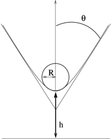
Figure 1: Configuration of hyperboloid and plate, illustrating the meaning of variables

The configuration is shown in Fig. 1. We choose units such that $\hbar=c=1$, and study the Casimir effects as functions of the variables $h$, $R$ and $\theta$. The limit $\theta\to 0$ at fixed $h$ and $R$ gives a paraboloid, $z=h+\rho^{2}/2R$, while $\theta\to\pi/2$ with finite $a$ is the planar limit.

III.2 Proximity force and semi-classical approximations

The proximity force approximation is a first approximation to the problem for arbitrary surfaces and is believed to give the most divergent term correctly in the limit of small distances, even though no rigorous proof for this exists. The PFA estimate is obtained by integrating the parallel plate result,

$$\frac{d{\cal E}}{dS}=-\frac{\pi^{2}}{1440z^{3}}$$ (8)

over one of the surfaces with $z$ replaced by the distance to the second surface measured normal to the first. In general, the PFA is ambiguous, since there are two choices for the integration surface and they yield, generically, different results. We choose to integrate over the planar surface, and obtain for the hyperboloid,

$${\cal E}_{\rm PFA}=-\int dS\frac{\pi^{2}}{1440z(\rho)^{3}}=-\frac{\pi^{3}R}{1440\ h^{2}}\left(1+\frac{h}{R}\tan^{2}\theta\right)\equiv-\frac{\pi^{3}R}{1440\ h^{2}}f_{\rm PFA}(h/R,\theta),$$ (9)

and we use the function $f(h/R,\theta)$ to present our results in general, so

$$f_{\rm PFA}(h/R,\theta)=1+\frac{h}{R}\tan^{2}\theta\,.$$ (10)

The conjecture that the PFA captures correctly the most divergent contribution in the limit $h\to 0$ translates to the conjecture that $f(0,\theta)=1$ is exact. We will see that both the optical and semi-classical approximations reproduce this relation.

A semi-classical approximation for the Casimir energy has been developed by Schaden and Spruch SandS following Gutzwiller’s methods Gutz . Like the optical approach this method identifies closed classical paths in the propagator $G$ and expands the functional integral about them. Unlike the optical approach, the trace of $G$ is calculated then by stationary phase leaving only periodic paths. In contrast, the optical approximation uses all closed and not necessarily periodic paths. This should be almost equivalent when only almost periodic paths contribute; however there are situations in which this is not true (see section III.4) and situations in which periodic paths do not exist, while closed paths do (inside a wedge, for example). The approaches are compared further in Ref. opt1 . The resulting semi-classical expression for the Casimir energy depends only on the local properties of the surface in the neighborhood of the points of reflection. For the hyperboloid, there is only one periodic path, the one that originates at the tip of the hyperboloid. In this case the approach of Schaden and Spruch gives

$$f_{\rm SS}(h/R,\theta) = \frac{90}{\pi^{4}}\frac{h}{R}\sum_{n=1}^{\infty}\frac{1}{n^{2}\sinh^{2}\left(n\,\log\left(\sqrt{1+\frac{h}{R}}+\sqrt{\frac{h}{R}}\right)\right)\,}$$ (11)

$$= 1-\frac{30}{\pi^{4}}\sum_{n=1}\left(\frac{1}{n^{2}}-\frac{1}{n^{4}}\right)\frac{h}{R}+{\cal O}\left((h/R)^{3/2}\right)$$

$$= 1-\frac{15-\pi^{2}}{3\pi^{2}}\frac{h}{R}+{\cal O}\left((h/R)^{3/2}\right)\,.$$

Notice that this result depends on $R$ but not on the angle $\theta$. In the semi-classical approximation the hyperboloid gives the same result as a sphere of radius of curvature $R$, irrespectively of the opening angle $\theta$. The next term in the power series is actually ${\cal O}\left((h/R)^{1+\alpha}\right)$ with $0<\alpha<1$. Numerically, we found $\alpha=1/2$. Notice that the term proportional to $h/R$ has the opposite sign from our computations and from the PFA prediction.

A priori we have no reason to dismiss either the PFA or the semi-classical approximation. Neither the $h/R$ nor the $\theta$ dependence of $f(h/R,\theta)$ is constrained by any general requirement. The only test we can foresee is either comparison with experiment or with a numerical computation after the manner of Ref. Gies03 . We believe that the optical approximation captures more of the relevant physics than either the PFA or semi-classical approximation. The PFA ignores the curvature of the surfaces entirely and the semi-classical approximation ignores the geometry except in the neighborhood of the periodic paths. We have already seen opt1 in the case of the sphere and the plate that the optical approximation gives a prediction for the coefficient of the linear term $h/R$ (where $R$ is the radius of the sphere) different from either the PFA or semi-classical approximations. The optical approximation differs significantly from the other approaches also in the case of a hyperboloid (the difference being more evident the smaller is the angular opening $\theta$ of the hyperboloid), so experiments or numerical computation will again have to provide discrimination among the approximations.

III.3 Optical approach data

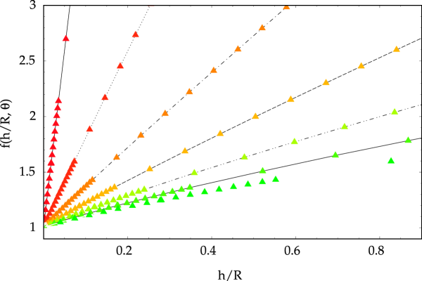
Figure 2: (Color online) Optical approximation for the function $f(h/R,\theta)$ versus $h/R$ for various openings of the hyperboloid $\theta$. From bottom up, azure to red, $\theta=20$ to $80$ degrees in steps of $10$ degrees. The function $A(\theta)$ is given by the slope at the origin.

We have computed the energy in the optical approximation up to 6 reflections with a numerical algorithm (see Appendix for details) for 7 different values of $\theta$ (from 20 to 80 degrees) and approximately 50 values of $h/R$ for each $\theta$. The data are presented in Fig. 2. For small $h/R$ we can expand $f$:

$$f(h/R,\theta)=1+A(\theta)h/R+\ldots\quad.$$ (12)

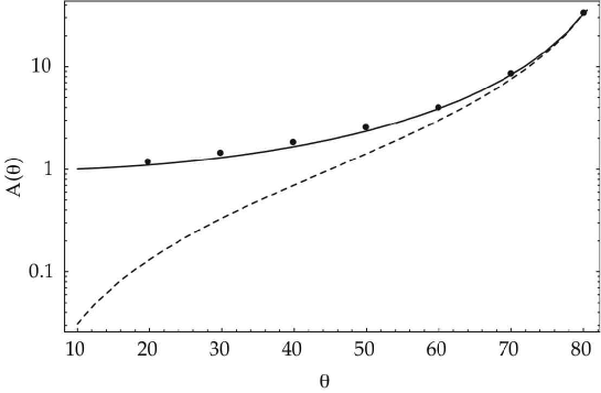
Figure 3: Optical approximation and PFA for $A(\theta)$. The continuous line is the function $1/\cos^{2}\theta$, the dashed line is the PFA prediction $\tan^{2}\theta$. $\theta=90^{o}$ is the parallel plates limit and the optical approximation agrees in its functional form with the PFA for large opening angles. The semi-classical prediction is $A=-0.17$ which cannot be displayed on a logarithmic scale.

This defines the function $A(\theta)$, which, for dimensional reasons, can only depend on $\theta$. The PFA gives only a term linear in $h/R$, $A_{{\rm PFA}}(\theta)=\tan^{2}\theta$. From Fig. 2 it is apparent that the optical approximation also is nearly linear in $h/R$ over the range of $h/R$ and $\theta$ shown. We have extracted this function from our data and plot it in Fig. 3.

As can be seen from the figure, the results of the optical approximation are well described by the function

$$A(\theta)=\frac{1}{\cos^{2}\theta}\,.$$ (13)

So far we have no explanation for this functional form. However, it is so simple and fits the data so accurately that it has probably a more profound meaning. To gain some further insight into this subject consider the limit $\theta\to 0$ at fixed finite $R$, in which the hyperboloid turns into a paraboloid with the radius of curvature equal to $R$. In this limit we obtain from eq. (13), $A_{\rm OPT}(0)=1$, whereas the PFA gives $A_{\rm PFA}(0)=0$, so the predictions for the paraboloid (hence the superscript para) differ dramatically,

$$f^{para}_{\rm OPT}(h/R,0) = 1+h/R+{\cal O}(h^{2}/R^{2}),$$ (14)

$$f^{para}_{\rm PFA}(h/R,0) = 1+{\cal O}(h^{2}/R^{2})\,.$$ (15)

Experimenters measure forces, not energies. The predictions for the Casimir force can be read off the figures for each of the approximations. The correspondence is particularly simple when $f(h/R,\theta)$ is approximated to linear order in $h/R$, as in eq. (12),

$${{\cal F}}=-\frac{d{\cal E}}{dh}=-\frac{\pi^{3}R}{720h^{3}}\left(1+\frac{h}{2R}A(\theta)+...\right)\,.$$ (16)

Another limit that is interesting in principle but cannot be analyzed within our approximation is the ‘cusp’ limit in which $R\to 0$ while $\theta$ is held fixed. Here, however, we face a major difficulty, since $h$ measured in units of $R$ is going to infinity, corresponding to the far right in Fig. 2. Since $h$ is the measure of the wavelengths that dominate the mode sum in eq. (1), the cusp limit is dominated by long wavelengths and diffraction (which is ignored in the optical approximation to the propagator) becomes more and more important.

III.4 Finite Plate Studies

The optical approximation allows one to study the effect of finite bounding surfaces. In the case of a hyperboloid it is not hard to extend our algorithm to the case when the plate is replaced by a finite disk of radius $L$. Since this is a configuration that may well be possible to examine experimentally, we work out the predictions of the optical approach and compare them with the PFA and the semi-classical approximation. In order to simplify the analysis we fixed $\theta=30^{\circ}$, though, of course, any other value of $\theta$ can be analyzed as well.

It is necessary to restrict ourselves to situations where $h\ll L,R$, in order to being able to neglect edge diffraction effects. However no restriction is posed on the relative magnitude of $R$ and $L$. In particular, the transition between $L>R$ and $R<L$ can be studied. One can think of the optical approximation as a semi-classical approximation to the Casimir energy for $h\ll L,R$ uniformly valid as a function of the parameter $R/L$ while the semi-classical approximation breaks down when $R/L\gtrsim 1$. This issue has been discussed in more general terms in paragraph III.C of Ref. opt1 .

If we factor out the most divergent term we can write

$${\cal E}=-\frac{\pi^{3}R}{1440h^{2}}g(h/R,L/R,\theta),$$

which is related to the function $f$, previously defined, by

$$f(h/R,\theta)=\lim_{L/R\to\infty}g(h/R,L/R,\theta)\,.$$ (17)

It is clear on physical grounds that if the radius of the finite plate, $L$, is small compared to the radius of curvature of the hyperboloid then the curvature of the hyperboloid can be neglected. In this case the result must reduce to that obtained for two parallel plates, one infinite and one of radius $L$,

$${\cal E}=-\frac{\pi^{3}L^{2}}{1440h^{3}}\,.$$ (18)

This implies that for $L/R\ll 1$ asymptotically one must find

$$g(h/R,L/R,\theta)\sim\frac{L^{2}}{hR}\,.$$ (19)

To gain a more complete understanding of the different regimes for varying $L/R$ and $h/R$ a good starting point is again the PFA, which has, as it will turn out, the same qualitative behavior as the optical approximation though it differs quantitatively. According to the PFA, for finite plate we have (here $\eta\equiv h/R,\ \lambda\equiv L/R$)

$$g_{\rm PFA}(\eta,\lambda,\theta)=\frac{\eta\,{\lambda}^{2}+{\cot^{2}\theta}\,\left({\lambda}^{2}+2\,\cot\theta\,\left(\cot\theta-{\sqrt{{\lambda}^{2}+{\cot^{2}\theta}}}\right)\right)}{{\left(\eta+{\cot^{2}\theta}\,\left(-1+{\sqrt{1+{\lambda}^{2}\,{\tan^{2}\theta}}}\right)\right)}^{2}}\,.$$ (20)

The expansion of this function in powers of $\eta$,

$$g_{\rm PFA}(\eta,\lambda,\theta) = 1+\eta\,{\tan^{2}\theta}\,$$ (21)

$$- \eta^{2}\frac{\left(6\,\cot^{2}\theta-6\,\cot\theta\,{\sqrt{\cot^{2}\theta+{\lambda}^{2}}}+{\lambda}^{2}\,\left(5-2\,{\sqrt{1+{\lambda}^{2}\tan^{2}\theta}}\right)\right)}{\cot^{6}\theta\,{\left(1-{\sqrt{1+\lambda^{2}\tan^{2}\theta}}\right)}^{4}}+{O(\eta)}^{3}$$

sheds considerable light on its non-uniform behavior. For any $\lambda$ (and $\theta$) it is possible to choose $\eta$ so small that the situation reverts to the hyperboloid opposite an infinite plate (i.e. the term of $O(\eta^{2})$ is negligible) and eq. (21) reduces to eq. (10). The fact that the coefficient of $\eta^{2}$ is proportional to $\lambda^{-4}$ when $\lambda\to 0$ signals non-uniform behavior in $\eta$ and $\lambda$. For small $\lambda$ the domain of linear growth with $\eta$ continues only up to $\eta\sim\lambda^{2}$ where $g$ has a maximum. For larger $\eta$ the expansion of eq. (20) in powers of $\eta$ breaks down and the small $\lambda$, finite parallel plate limit of eq. (19) applies, so expanding $g$ in powers of $\lambda^{2}/\eta$ we find

$$g_{\rm PFA}\sim\frac{{\lambda}^{2}}{\eta}-\frac{3\,{\lambda}^{4}}{4\,{\eta}^{2}}+{{\cal O}\left(\frac{\lambda^{6}}{\eta^{3}}\right)},$$ (22)

whose first term, once $h,R$ and $L$’s have been restored, coincides with eq. (19). For $\lambda\lesssim 1$ the achievement of the maximum in $\eta$ represents the set-in of the parallel plate limit: i.e. $R$ is large with respect to $L$ and $h$ is large enough that the contribution to the energy is not too much concentrated near the tip. When $\lambda\gtrsim 1$ even though we cannot neglect the curvature over distances of order $L$ the contribution to the energy is spread enough so that the parallel plates approximation works again. However in this region we expect curvature effects (not captured by PFA) to be non-negligible. Here hence we expect – and we find – the biggest differences between the optical data and PFA.

The semi-classical approximation does not predict any change in the energy with the plate radius $L$ and hence cannot predict the parallel plates limit. This is due to the fact that the only semi-classical contribution comes from the periodic orbit bouncing back and forth from the tip of the hyperboloid to the plate and this ignores completely the transverse radial direction. This becomes pathological in the case when the geometry reduces to that of two parallel plates, where it gives completely wrong results. Explicitly, it predicts an energy ${\cal E}\propto\hbar cR/h^{2}$ while the correct result is independent of $R$.

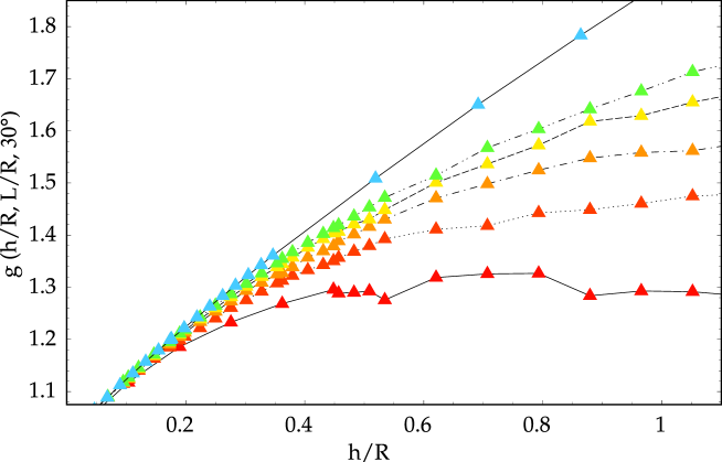
Figure 4: (Color online) The function $g(h/R,L/R,\theta)$ given by the optical approximation. $\theta=30^{\circ}$ for all of the curves. From down to up (red to green) the first five set of points have $L/R=$ $1.5\sqrt{3}$, $2.0\sqrt{3}$, …, $3.5\sqrt{3}$, the blue triangles (uppermost curve) are the infinite plate case. The wiggles for large $h/R$ and small $L/R$ are related to the accuracy of our computation, and are smoothed out to a large extent when we increase the accuracy.

With these considerations in mind we now turn to the results of the optical approximation. The optical approximation to $g$ is shown for various values of $L/R$ as a function of $h/R$ in Fig. 4. The linear term in an expansion in $h/R$ at fixed $L/R$ (previously called $A$) does not depend on $L$. This result is shared with the PFA (see eq. (21)) and the semi-classical approximation, which is completely independent of $L$. However, the general dependence on $h/R$ is completely different. This can be seen graphically in Fig. 5.

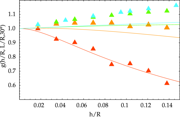
Figure 6: (Color online) Comparison of the optical approximation and PFA for $g(h/R,L/R,\theta)$ for $\theta=30^{\circ}$ and various $L/R$ as a function of $h/R$. From down up (red to blue) $L/R=\sqrt{3}/4,\sqrt{3}/2,\sqrt{3},2\sqrt{3}.$ The continuous lines are the PFA predictions. The $L/R=\sqrt{3}/4$, red data are fitted by the PFA within error bars (not shown) and the larger the plate the worse the agreement.

Returning to Fig. 4, we see that the optical approximation predicts variation of $g$ with $L/R$ for $h/R\lesssim 1$. The $L$ dependence of the PFA agrees quantitatively with the optical approach for $h/R\ll 1$ and in the parallel plate limit, where they both predict $g\to L^{2}/hR$. However they differ in the intermediate range of $h/R$ and $L/R$. In Fig. 6 we compare the $L/R$ dependence predicted by the optical approximation with the PFA. For the smallest value of $L/R$ ($L=\sqrt{3}R/4$), the two agree within the error bars on the optical data both at very small $h/R$ and larger $h/R$ where they both approach the “parallel plate” regime. This is the more evident manifestation of the uniform validity of the optical approximation as the geometry is changed. Notice that the agreement becomes worse as $L$ is increased. This makes it clear that PFA only captures correctly a small region around the tip of the hyperboloid, where the paths are almost periodic. Even here it ignores the enlargement factor. Continuing to increase $L$ at fixed $h$, we enter the region $h\ll L^{2}/R$, where $g$ reduces to the infinite plate prediction and the slopes of optical and PFA curves will differ according to the previous discussion.

The optical approximation, like the PFA, predicts a maximum in $g(h/R,L/R,\theta)$ as a function of $h/R$ at fixed $L/R$. The maximum of $g$ for fixed $L/R$ and $\theta$ is already evident in Fig. 4 for $L=1.5\sqrt{3}R$. It occurs for every finite $L/R$ — even though this cannot be seen in Fig. 4. We will call this value $g^{*}(L/R,\theta)$, and the value of $h/R$ at which this is found will be $\eta^{*}(L/R,\theta)$. For $L/R\gtrsim 1.5\sqrt{3}$ the maximum occurs in a region of $h/R$ that is beyond the applicability of our approximation ($h^{*}/R\gtrsim 1$).

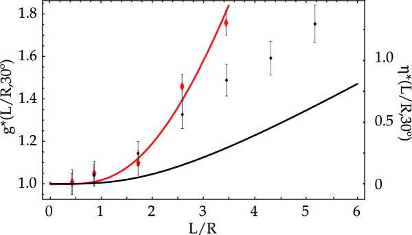
Figure 7: (Color online) The lower, black curve is the PFA prediction for $g^{*}(L/R,\theta)$, the maximum of $g(h/R,L/R,\theta)$ as a function of $L/R$ and the black points are the optical results. The upper, red curve is PFA prediction for $h^{*}/R=\eta^{*}(L/R,\theta)$, the value of $h/R$ at which the maximum occurs, as a function of $L/R$, and the red points are optical data. Both curves have $\theta=30^{\circ}$. The optical approximation data carry an error bar of $~{}5\%$ on $g^{*}$ and $0.1$ on $\eta^{*}$, estimated from the accuracy of the numerical integration and the maximum finding procedure.

We present the data for $g^{*}$ and $\eta^{*}$ in Fig. 7. The data on $\eta^{*}$ are in good agreement with the PFA prediction. The data on $g^{*}$, however, are in worse accord. One could then say that PFA and the optical approximation disagrees on the predictions for the energy (and hence the force) but they agree in identifying the basic length scales of the problem.

In conclusion, there are also important differences among the various approximations when applied to the finite plate case. These differences are more marked than in the infinite plate case. In particular the semi-classical approach SandS does not depend on the size of the plate (nor on that of the hyperboloid) at all. For finite $L$ the optical approximation data for $g$ reach a maximum and then decrease. This is not captured by the semi-classical approximation and is understood by the PFA only qualitatively but not quantitatively.

IV Conclusions

Studies of the geometrical dependence of Casimir forces are in their infancy. Experiments are just reaching the level of accuracy where deviations from the naive proximity force approximation can be detected. There are few theoretical calculations for geometries other than parallel plates. The optical approximation offers hope for an accurate estimate of Casimir forces for a wide range of geometries. However we do not know how to bound the corrections to this approximation. The configuration of a hyperboloid and plate offers a flexible laboratory for studying approximations. It is likely to be accessible to experiment. One should keep in mind, however, that actual experiments involve electromagnetic fields not scalar fields. In the case of parallel plate the only modification is an increase of the force by a factor of two. For curved surfaces the effect is not so well understood, but the dominant effect is still simply a factor of two.

The goal of this paper has been to work out the predictions of the optical approach so they can be compared with experiment and contrasted with other approximations. We find that the optical approximation differs significantly from the PFA and the semi-classical approximation. The difference becomes more important as the opening angle of the hyperboloid, $\theta$, decreases. All approximations agree on the first term in an expansion in $h/R$, but differ thereafter. We certainly expect the optical approach to be more accurate, but in the absence of an estimate of errors, only comparison with experiment or with a numerical computation in the spirit of Ref. Gies03 can settle the issue. We have also studied the effects of replacing the infinite planar plate with a finite disk. We found notable differences both with PFA and the semi-classical approximation of SandS . In some domains of the parameters $h,L,R$ these differences are so relevant that we believe they can be easily measured in an actual experiment.

More generally speaking, the high precision experiments to be performed in the near future will be able to measure the next-to leading order terms in a small distance expansion and will hence be able to tell us whether the recent developments in the theoretical analysis of Casimir effects for curved geometries point in the right direction.

V Acknowledgements

We thank G. L. Klimchitskaya and V. M. Mostepanenko for helpful discussions. O. S. gratefully acknowledges conversations with K. Fukushima. O. S. was supported by the Deutsche Forschungsgemeinschaft under grant DFG Schr 749/1-1. A. S. is Bruno Rossi Fellow and Jonathan A. Whitney Fellow, partially supported by INFN. This work is also supported in part by funds provided by the U.S. Department of Energy (D.O.E.) under cooperative research agreement DF-FC02-94ER40818.

VI Appendix

We have developed a C-program that allows one to calculate the optical contribution to the Casimir energy. In this Appendix we discuss the algorithm in some detail because we believe it may be relevant for other problems, such as the study of density of states oscillations in chaotic billiards.

VI.1 Outline

The starting point of the numerical computations in this paper is eq. (4) which we repeat here for convenience:

$${\cal E}_{\rm optical}=-\frac{\hbar c}{2\pi^{2}}\sum_{\bf n}(-1)^{n}M_{n}\int_{{\cal D}_{\bf n}}d^{3}x\frac{\sqrt{\Delta_{\bf n}(x)}}{\ell_{\bf n}^{3}(x)}\,.$$ (23)

From this equation, it is obvious which kind of question a numerical program has to address. Performing the sum over ${\bf n}$ is a trivial task since we consider only paths with a fixed upper bound on the number of reflections, in our case six. The second ingredient is a routine that performs the spatial integration. Since the surfaces we have are cylindrically symmetric, we introduce cylindrical coordinates, and carry out the integration over $\varphi$. Then we are left with an integral over $z$ and over $\rho$. Both integrations are done using an adaptive step size differential equation solver, in our case a slightly modified version of odeint NumericalRecipes . The integration routine will choose a number of points where the path length $\ell_{\bf n}$ and the enlargement factor $\Delta_{\bf n}$ are required. In order to compute these quantities, the optical paths are needed. These paths are closed paths of minimum length, specified by the bulk point they start from, the number of reflections and the sequence of surfaces they reflect from. The requirement that they be of minimum length is equivalent to saying that they are - between reflections - straight, and the reflections are specular. The way we determine these paths will be treated extensively below. Once an optical path is determined, it is obviously trivial to determine its length. It is also a simple matter to determine the enlargement factor, as will also be described in some detail below. As a last point, it should be mentioned that the determination of the integration domain is rather implicit. Formally, we integrate over the volume enclosed between the two surfaces (except for the one-reflection term pap1 ). The reduction of this volume to ${\cal D}_{\bf n}$ comes about because for some points in the volume no closed path with specular reflections only exists. Hence, if our routines for finding minimum paths do not find any, the contribution of this point to the integral is set to zero.

VI.2 Minimum Paths and Subtleties

The integration routine chooses points in the bulk where path length and enlargement factor are required. Since it is known that a path of minimum length will have — at each reflection — incoming and outgoing angles identical, the determination of a minimum length path is a one parameter minimization problem. There are (at least) two different approaches to determine the path of minimum length, both of which are used in our numerical procedure. Either, the $n$-reflection path under consideration is allowed to be open, but all reflections are specular (“open path approach”), or the path is required to be closed, but then the last reflection is not required to be specular (“path length minimization approach”):

• Open path approach (cf. left-hand panel of fig. 8): Here we consider the path generated by a sequence of specular reflections. Such a path will, in general, not return to the point at which it originated. Consider the piece of path that is obtained after n reflections. Then consider the point on this piece of path that has the minimum distance (labeled final A and final B in the figure) from the point in the bulk where this path originated from (labeled bulk in the figure). Minimize this minimum distance by varying the point of the first reflection (choices labeled 1A, 1B in the figure). The minimum of this function is zero, and if a zero is found the path is indeed a closed path where all reflections are specular. Numerically, it is easier to find a zero crossing than a minimum, therefore it is useful to define a signed distance, i.e. a distance that has a notion of whether the last piece of the path passes above the bulk point or below; some details on this will be given below. We use the abbreviation SDZC (‘signed distance zero crossing’) for this method.

• Path length minimization (cf. right-hand panel of fig. 8): In this case we insist that the paths be closed but give up the constraint that all reflections have to be specular. In general, if we insist on the path being closed all reflections can be chosen to be specular save the last one. Thus we reflect the path $n-1$ times, and note where the $n^{\rm th}$ reflection would have occurred. Then we minimize the length of the path as a function of the initial reflection point. We use the abbreviation PLM (‘path length minimization’) for this method.

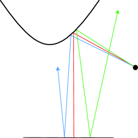
Figure 9: (Color online) This figure illustrates the subtlety described in the text regarding the possibility of a sign change of the signed distance function without finding a closed path. The black dot indicates the bulk point. The middle path (red) is the path that detects the singularity in the sign function used.

Both methods have advantages and disadvantages. The advantage of the SDZC method is that if it works, then it works much faster, since the zero crossings of the signed distance function are much steeper than the minima of the path length function. However, if one wants to keep the determination of the sign in the SDZC method simple, there are cases where – as the initial point is varied – the sign changes, but apparently not continuously, i.e. the signed distance can not be made arbitrarily small. This counter-intuitive behavior is best understood with a specific example (see Figure 9). In order to determine the sign we follow the last part of the path till it has the same value of $\rho$ as the bulk point where the path started from. Then we compare the $z$ coordinate of this point on the path with the $z$ coordinate of the bulk point and we can say whether the path passes above or below the bulk point. In order to understand how one gets a sign change without finding a closed path, consider a two-reflection path with the first reflection off the hyperbola (situation in Figure 9). If this path reflects off the plate perpendicularly, it has found the singularity in our sign prescription. Since this last part of the path can never have the $\rho$ value of the bulk point, it cannot be decided whether it passes above or below. This is the underlying cause for the sign change without a zero crossing of the signed distance function: if instead of this singular path we consider a path with initial point on the hyperbola to the left (resp. right), the part of the path reflecting off the plate will be reflected also to the left (right) and hence passing below (above) the bulk point.

If no closed path can be found using the SDZC method we use the PLM instead. Both methods also have to deal with difficulties that are not apparent in Fig. 8. There we have shown two reflection paths only, and the problems appear significantly first for four reflection paths. First, a problem for the SDZC method is that given the initial point, an $n$ reflection path might not exist if anywhere in between a piece of path does not “hit” the designated next surface but simply runs off to infinity. Second, a problem for the PLM is that either the first section of the path or the last section of the path may intersect one of the surfaces, thus rendering the path illegal. A useful method of handling these paths is to ensure that they have a length that is (orders of magnitude) larger than the largest “correct” length that can appear in the problem, though still finite. In the first case, this is ensured by terminating the section of the path that does not hit a surface at a very large distance, in the second case a large number is added to the otherwise ordinarily computed path length. The subtlety is that on the one hand this large number should be much larger than any path length occurring, so that an illegal path can be spotted by simply looking at its length. However, the number should not be so big that – with the prescribed numerical accuracy – the finite length information of the path length is lost. The reason for this requirement is that for sufficiently many reflections (and this is a serious problem already at six reflections) almost all paths run off to infinity. If the finite information is destroyed by the value we choose for the large number, the PLM has no variation of path length to work on. However, such a variation of the path length is needed since the PLM works in the following way: first, path lengths for a finite number of initial points with $\rho$ values slightly above the $\rho$ value of the bulk point down to $\rho=0$ are computed. Then within these points one searches for the region where there has to be a minimum. In other word one looks for three points $\rho_{1}<\rho_{2}<\rho_{3}$ with $length(\rho_{2})<length(\rho_{3})$ and $length(\rho_{2})<length(\rho_{1})$). Once this region is identified, the true minimum is found by Golden Section Search NumericalRecipes ). For example in double precision C$++$, $10^{30}$ is too big, whereas $10^{10}$ is just the right size for the large number.

VI.3 Enlargement Factors

The computation of the enlargement factor is rather simple once the first reflection point of a closed minimum path has been found: take a step of unit length from the point in the bulk towards the first point of reflection. From the point thus reached construct four new points: by going $\epsilon$ into positive and negative $y$ direction (usually our computations take place in the $x-z$ plane, therefore a step in $y$ and $-y$ is guaranteed to be orthogonal), and a step each into the direction orthogonal both to the $y$ axis and the direction where we took our first unit step. These four points define four new paths: they start at the original bulk point, and pass through these four new points. Then – in case we are considering an $n$ reflection path – they are reflected $n$ times off the proper surfaces. These paths will not be closed since we consider only convex surfaces. After $n$ reflections we determine the points of minimum distance to the bulk point. These four points together with the bulk point determine four triangles. Their areas are added up to give $dA$, whereas $d\Omega=2\epsilon^{2}$.

This procedure is numerically very convenient, since in order to find the path of minimum length for each bulk point a couple of hundred paths have to be computed, but once it is found, only four more paths need to be computed for the enlargement factor (Fig. 10).

We have tested that this procedure produces stable results for generic bulk points for widely varying values of $\epsilon$ between $10^{-8}$ and $10^{-3}$.

Figure 5: Comparison of $g(h/R,L/R,\theta)$ given by the optical approximation (triangles), the PFA (continuous) and semi-classical result (dashed curve). $\theta=30^{\circ}$ and $L=2\sqrt{3}R$ for all the curves.

         

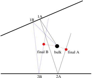
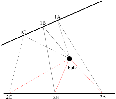
Figure 8: (Color online) The left panel shows how the “open path approach” works, the right panel shows the procedure in the “path length minimization”. In the left panel, all reflections have equal incoming and outgoing angles; in the right panel only the reflections at points 1A,1B,1C have equal incoming and outgoing angles.

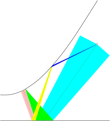
Figure 10: (Color online) Computation of the enlargement factor for the example of a four reflection path. The dotted line indicates the closed minimum length path for which the enlargement factor is computed.

References

- (1) H. B. G. Casimir, Proc. K. Ned. Akad. Wet. 51, 793 (1948).
- (2) S. K. Lamoreaux, Phys. Rev. Lett. 78, 5 (1997); For a review, see M. Bordag, U. Mohideen and V. M. Mostepanenko, Phys. Rept. 353, 1 (2001) [arXiv:quant-ph/0106045]; For more recent experimental results see G. Bressi, G. Carugno, R. Onofrio and G. Ruoso, Phys. Rev. Lett. 88, 041804 (2002) [arXiv:quant-ph/0203002]
- (3) R. S. Decca, E. Fischbach, G. L. Klimchitskaya, D. E. Krause, D. L. Lopez and V. M. Mostepanenko, Phys. Rev. D 68, 116003 (2003) [arXiv:hep-ph/0310157].
- (4) B. V. Derjagin, Kolloid Z. 69 155 (1934), B. V. Derjagin, I. I. Abriksova, and E. M. Lifshitz, Sov. Phys. JETP 3, 819 (1957); For a modern discussion of the Proximity Force Theorem, see J. Blocki and W. J. Swiatecki, Annals Phys. 132, 53 (1981).
- (5) A. Scardicchio and R. L. Jaffe, Nucl. Phys. B 704, 552 (2004) [arXiv:quant-ph/0406041].
- (6) R. L. Jaffe and A. Scardicchio, Phys. Rev. Lett. 92, 070402 (2004) [arXiv:quant-ph/0310194].
- (7) H. Gies, K. Langfeld and L. Moyaerts, JHEP 0306, 018 (2003) [arXiv:hep-th/0303264].
- (8) M. Schaden and L. Spruch, Phys. Rev. A 58, 935 (1998); Phys. Rev. Lett. 84, 459 (2000).
- (9) M. C. Gutzwiller, J. Math. Phys.12, 343 (1971); Chaos in Classical and Quantum Mechanics, Springer, Berlin (1990).
- (10) N. Graham, R. L. Jaffe, V. Khemani, M. Quandt, O. Schroeder and H. Weigel, Nucl. Phys. B 677, 379 (2004) [arXiv:hep-th/0309130].
- (11) N. Graham, R. L. Jaffe, V. Khemani, M. Quandt, M. Scandurra and H. Weigel, Nucl. Phys. B 645, 49 (2002) [arXiv:hep-th/0207120].
- (12) M. Klein and I. W. Kay Electromagnetic theory and geometrical optics, Interscience, N.Y. (1965).
- (13) W. H. Press, S. A. Teukolsky, W. T. Vetterling, B. P. Flannery Numerical Recipes in C++, Cambridge University Press, (2002)