How Phase Transitions induce classical behaviour

Abstract

We continue the analysis of the onset of classical behaviour in a scalar field after a continuous phase transition, in which the system-field, the long wavelength order parameter of the model, interacts with an environment, of its own short-wavelength modes and other fields, neutral and charged, with which it is expected to interact. We compute the decoherence time for the system-field modes from the master equation and directly from the decoherence functional (with identical results). In simple circumstances the order parameter field is classical by the time the transition is complete.

03.70.+k, 05.70.Fh, 03.65.Yz

I Introduction

The standard big bang cosmological model of the early universe assumes a period of rapid cooling, giving a strong likelihood of phase transitions, at the grand unified and electroweak scales Kolb in particular.

In this talk we describe how phase transitions naturally take us from a quantum to classical description of the universe. Metaphysics aside, cosmologists rely on the fact that the relevant fields obey classical equations from early times, since it is not possible to solve the quantum theory directly. Fortunately, we have reason to believe that (continuous) transitions will move us rapidly to classical behaviour. Classical behaviour arises in the following way:

• Classical correlations: By this is meant that the Wigner function(al) $W[\pi,\phi]$ peaks on classical phase-space trajectories, with a probabilistic interpretation.

• Diagonalisation: By this is meant that the density matrix $\rho(t)$ should become (approximately) diagonal, in this case in a field basis. Alternatively, we can demand diagonalisation of the decoherence functional. In either case a probabilistic description (no quantum interference) is obtained.

• Stochastic behaviour: The decoherence functional, which provides the diffusion (noise) to diagonalise the density matrix also supplies the dissipation that enables the fields to obey probabilistic stochastic equations, which evolve into classical equations.

From the papers of Guth and Pi guthpi onwards, it has been appreciated that unstable modes lead to classical correlations through squeezing. On the other hand, we understand diagonalisation to be an almost inevitable consequence of tracing over the ’environment’ of the ’system’ modes.

Continuous transitions supply both ingredients, from which the classical equations follow. Firstly, the field ordering after such a transition is due to the growth in amplitude of unstable long-wavelength modes, which arise automatically from unstable maxima in the potential. Secondly, the stable short-wavelength modes of the field, together with all the other fields with which it interacts, form an environment whose coarse-graining enforces diagonalisation and makes the long-wavelength modes decohere.

What matters are the time scales. An ideal situation, which we shall show is possible, is that the theory becomes classical in the sense above, before the transition is complete. However, to quantify this is difficult because, with fields, we are dealing with infinite degree of freedom systems. One of us (F.L) has shown elsewhere diana how classical correlations arise in quantum mechanical systems that mimic the field theory that we shall consider here, and we refer the reader to that paper for the role that classical correlations play. Our concern in this talk is, rather, with diagonalisation, determined both through the master equation for the evolution of the density matrix and the decoherence functional, whose role is to describe consistent histories. Stochastic equations are then a corollary to this same diagonalisation.

This talk builds upon earlier published work by us and Diego Mazzitelli lomplb ; lomplb2 ; lomnpb , together with our contributions to the proceedings of the 2001 meeting in Peyresq P1 ; P2 and we refer the reader to this earlier work for much of the basic technical details. We restrict ourselves to flat space-time. The extension to non-trivial metrics is straightforward in principle. See the recent work of Lombardo POFer , which complements this. The developments since the last proceedings are our greater understanding of the use of trial configurations and slower quenches lomnpb , the parallel use of the decoherence functional to characterise decoherence, and the extension of the theory to include electromagnetism ubaIC .

II Evolution of the density matrix

The evolution of a quantum field as it falls out of equilibrium at a transition is determined in large part by its behaviour at early times, before interactions have time to take effect. To be concrete, consider a real scalar field $\phi(x)$, described by a $Z_{2}$-symmetry breaking action ($\mu^{2}>0$)

$$S[\phi]=\int d^{4}x\left\{\frac{1}{2}\partial_{\mu}\phi\partial^{\mu}\phi+\frac{1}{2}\mu^{2}\phi^{2}-\frac{\lambda}{4!}\phi^{4}\right\},$$ (1)

with symmetry breaking scale $\eta^{2}=6\mu^{2}/\lambda$. On heating, this shows a continuous transition, with critical temperature $T_{\rm c}^{2}=2\eta^{2}$. If, by virtue of the expansion of the universe the system is very rapidly cooled (quenched) from $T>T_{\rm c}$ to $T<T_{\rm c}$, the initial stages of the transition can be described by a free field theory with inverted mass $-\mu^{2}<0$. The state of the field is initially concentrated on the local maximum of the potential, and spreads out with time. This description is valid for short times, until the field wave functional explores the ground states of the potential.

The $\phi$-field ordering after the transition is due to the growth in amplitude of its unstable long-wavelength modes, which we term $\phi_{<}(x)$. For an instantaneous quench these have wave-number $k<\mu$ for all time. Although the situation is more complicated for slower quenches, until the transition is complete there are always unstable modes. As a complement to these, we anticipate that the stable short-wavelength modes of the field $\phi_{>}(x)$, where

$$\phi(x)=\phi_{<}(x)+\phi_{>}(x),$$

will form an environment whose coarse-graining makes the long-wavelength modes decohere fernando . In practice, the boundary between stable and unstable is not crucially important, provided there is time enough for the power in the field fluctuations to be firmly in the long-wavelength modes. This requires weak coupling $\lambda\ll 1$. Of course, all the other fields with which $\phi$ interacts will contribute to its decoherence, but for the moment we ignore such fields (before returning to them in the last section).

After splitting, the action (1) can be written as

$$S[\phi]=S[\phi_{<}]+S[\phi_{>}]+S_{\rm int}[\phi_{<},\phi_{>}],$$ (2)

where the interaction term is dominated lomplb ; lomnpb by its biquadratic term

$$S_{\rm int}[\phi_{<},\phi_{>}]\approx-\frac{1}{6}\lambda\int d^{4}x~{}\phi_{<}^{2}(x)\phi_{>}^{2}(x).$$ (3)

The total density matrix (for the system and bath fields) is defined by

$$\rho_{\rm r}[\phi^{+},\phi^{-},t]=\rho[\phi_{<}^{+},\phi_{>}^{+},\phi_{<}^{-},\phi_{>}^{-},t]=\langle\phi_{<}^{+}\phi_{>}^{+}|{\hat{\rho}}|\phi_{<}^{-}\phi_{>}^{-}\rangle,$$

and we assume that, initially, the thermal system and its environment are not correlated.

On tracing out the short-wavelength modes, the reduced density matrix

$$\rho_{\rm r}[\phi_{<}^{+},\phi_{<}^{-},t]=\int{\cal D}\phi_{>}\rho[\phi_{<}^{+},\phi_{>},\phi_{<}^{-},\phi_{>},t],$$

whose diagonalisation determines the onset of classical behaviour, evolves as

$$\rho_{\rm r}[t]=\int d\phi_{<\rm i}^{+}\int d\phi_{<\rm i}^{-}~{}J_{\rm r}[t,t_{\rm i}]~{}\rho_{\rm r}[t_{\rm i}],$$

where $J_{\rm r}[t,t_{\rm i}]$ is the evolution operator

$$J_{\rm r}[t,t_{\rm i}]=\int_{\phi_{<\rm i}^{+}}^{\phi_{<\rm f}^{+}}{\cal D}\phi_{<}^{+}\int_{\phi_{<\rm i}^{-}}^{\phi_{<\rm f}^{-}}{\cal D}\phi_{<}^{-}\exp\{iS_{CG}[\phi_{<}^{+},\phi_{<}^{-}]\}.$$ (4)

$S_{CG}[\phi_{<}^{+},\phi_{<}^{-}]$ is the coarse-grained effective action, of the closed time-path form

$$S_{CG}[\phi_{<}^{+},\phi_{<}^{-}]=S[\phi_{<}^{+}]-S[\phi_{<}^{-}]+\delta S[\phi_{<}^{+},\phi_{<}^{-}].$$

All the information about the effect of the environment is encoded in $\delta S[\phi_{<}^{+},\phi_{<}^{-}]$ through the influence functional (or Feynman-Vernon functional feynver )

$$F[\phi_{<}^{+},\phi_{<}^{-}]=\exp\{i\delta S[\phi_{<}^{+},\phi_{<}^{-}]\}.$$

$\delta S$ has a well defined diagrammatic expansion, of the form

$$\delta S[\phi_{<}^{+},\phi_{<}^{-}]=\langle S_{\rm int}[\phi_{<}^{+},\phi_{>}^{+}]\rangle-\langle S_{\rm int}[\phi_{<}^{-},\phi_{>}^{-}]\rangle$$

$$+{i\over{2}}\{\langle S_{\rm int}^{2}[\phi_{<}^{+},\phi_{>}^{+}]\rangle-\big{[}\langle S_{\rm int}[\phi_{<}^{+},\phi_{>}^{+}]\rangle\big{]}^{2}\}$$

$$-i\langle S_{\rm int}[\phi_{<}^{+},\phi_{>}^{+}]S_{\rm int}[\phi_{<}^{-},\phi_{>}^{-}]\rangle$$

$$+i\langle S_{\rm int}[\phi_{<}^{+},\phi_{>}^{+}]\rangle\langle S_{\rm int}[\phi_{<}^{-},\phi_{>}^{-}]\rangle$$

$$+{i\over{2}}\{S^{2}_{\rm int}[\phi_{<}^{-},\phi_{>}^{-}]\rangle-\big{[}\langle S_{\rm int}[\phi_{<}^{-},\phi_{>}^{-}]\rangle\big{]}^{2}\}.$$ (5)

The quantum averages of the functionals of the fields are with respect to the free field action of the environment, defined as

$$\langle B[\phi_{>}^{+},\phi_{>}^{-}]\rangle=\int d\phi_{>\rm i}^{+}\int d\phi_{>\rm i}^{-}~{}\rho_{>}[\phi_{>\rm i}^{+},\phi_{>\rm i}^{-},t_{0}]$$

$$\times\int d\phi_{>\rm f}^{+}\int_{\phi_{>\rm i}^{+}}^{\phi_{>\rm f}^{+}}{\cal D}\phi_{>}^{+}\int_{\phi_{>\rm i}^{-}}^{\phi_{>\rm f}^{-}}{\cal D}\phi_{>}^{-}$$

$$\times\exp{{i\over{\hbar}}\{S_{0}[\phi_{>}^{+}]-S_{0}[\phi_{>}^{-}]\}}B[\phi_{>}^{+},\phi_{>}^{-}].$$

To lowest order $\lambda^{2}$ diagrams are one-loop in the short wavelength modes.

II.1 The Master Equation

Once the reduced density matrix has become approximately diagonal quantum interference has effectively disappeared and the density matrix permits a conventional probability interpretation. To see how the diagonalisation of $\rho_{\rm r}$ occurs, we construct the master equation, which casts its evolution in differential form. As a first approximation, we make a saddle-point approximation for $J_{\rm r}$ in Eq.(4),

$$J_{\rm r}[\phi_{<{\rm f}}^{+},\phi_{<{\rm f}}^{-},t_{f}|\phi_{<{\rm i}}^{+},\phi_{<{\rm i}}^{-},t_{i}]\approx\exp(iS_{CG}[\phi^{+}_{<\rm cl},\phi^{-}_{<\rm cl}]),$$ (6)

In (6) $\phi^{\pm}_{<\rm cl}$ is the solution to the equation of motion

$$\frac{\delta ReS_{CG}}{\delta\phi_{<}^{+}}\bigg{|}_{\phi_{<}^{+}=\phi_{<}^{-}}=0,$$

with boundary conditions $\phi^{\pm}_{\rm cl}(t_{0})=\phi^{\pm}_{<\rm i}$ and $\phi^{\pm}_{<\rm cl}(t)=\phi^{\pm}_{<\rm f}$.

It is very difficult to solve this equation analytically. We exploit the fact that, even if the universe is completely homogeneous prior to the transition then, after the transition, causality requires kibble that it be inhomogeneous because of the finite speed at which the order parameter fields can order themselves. This is in contra-distinction to the usual adiabatic analysis in which (for the continuous transition that interest us here) the correlation length diverges at the transition.

Since the field cannot be homogeneous in either of its groundstates $\phi=\eta$ or $\phi=-\eta$ there is an effective ’domain’ structure in which the domain boundaries are ’walls’ across which $\phi$ flips from one groundstate to the other. Further, these domains have a characteristic size $\xi$, where $\xi^{-1}=\pi k_{0}$ labels the dominant momentum in the power of the $\phi$-field fluctuations as the unstable long-wavelength modes grow exponentially. For simplicity, we adopt a ’minisuperspace’ approximation, in which we assume regular domains, enabling $\phi_{<\rm cl}(\vec{x},s)$ to be written as

$$\phi_{<\rm cl}(\vec{x},s)=f(s,t)\Phi(x)\Phi(y)\Phi(z),$$ (7)

where $\Phi(0)=\Phi(\xi)=0$, and

$$\Phi(x+\xi)=-\Phi(x).$$

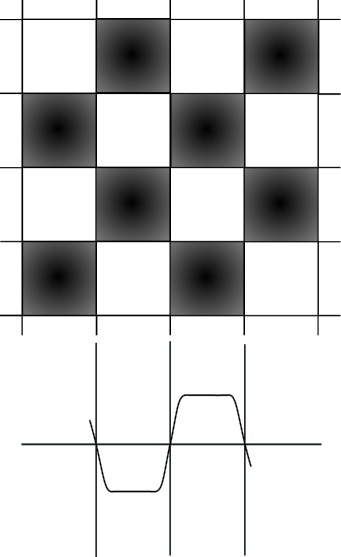
Figure 1: The field profile (7) in two dimensions, with lattice size $\xi$. Dark areas represent $\phi\approx\eta$, light areas $\phi\approx-\eta$. The boundaries are domain walls, with profile given below.

$f(s,t)$ satisfies $f(0,t)=\phi_{<\rm i}$ and $f(t,t)=\phi_{<\rm f}$. We write it as

$$f(s,t)=\phi_{<\rm i}u_{1}(s,t)+\phi_{<\rm f}u_{2}(s,t).$$ (8)

In lomnpb we made the simplest choice for $\Phi(x)$,

$$\Phi(x)=\cos k_{0}x.$$

Extensions to include more Fourier modes are straightforward in principle, but our work in lomnpb was sufficient to show that the results only depend weakly on the details of the domain function $\Phi(x)$ for few Fourier modes. In the light of the more qualitative comments made here, we refer the reader again to lomnpb for details. On the other hand, the $u_{i}(s,t)$ are solutions of the mode equation for wavenumber $k_{0}$ during the quench, with boundary conditions $u_{1}(0,t)=1$, $u_{1}(t,t)=0$ and $u_{2}(0,t)=0$, $u_{2}(t,t)=1$.

In order to obtain the master equation we must compute the final time derivative of the propagator $J_{\rm r}$. After that, all the dependence on the initial field configurations $\phi^{\pm}_{\rm i}$ (coming from the classical solutions $\phi^{\pm}_{\rm cl}$) must be eliminated. Assuming that the unstable growth has implemented diagonalisation before back-reaction is important, $J_{\rm r}$ can be determined, approximately, from the free propagators as

$$J_{0}[t,t_{\rm i}]=\int_{\phi_{<\rm i}^{+}}^{\phi_{<\rm f}^{+}}{\cal D}\phi_{<}^{+}\int_{\phi_{<\rm i}^{-}}^{\phi_{<\rm f}^{-}}{\cal D}\phi_{<}^{-}\exp\{i[S_{0}(\phi_{<}^{+})-S_{0}(\phi_{<}^{-})]\}$$ (9)

where $S_{0}$ is the free-field action. This satisfies the general identities fernando

$$\phi^{\pm}_{\rm cl}(s)J_{0}=\Big{[}\phi^{\pm}_{\rm f}[u_{2}(s)-\frac{{\dot{u}}_{2}(t)}{{\dot{u}}_{1}(t)}u_{1}(s)]\mp i{u_{1}(s)\over{{\dot{u}}_{1}(t)}}\partial_{\phi^{\pm}_{<\rm f}}\Big{]}J_{0}$$

which allow us to remove the initial field configurations $\phi^{\pm}_{\rm i}$, and obtain the master equation.

Even with these simplifications the full equation is very complicated, but it is sufficient to calculate the correction to the usual unitary evolution coming from the noise (diffusion) kernels (to be defined later). The result reads

$$i{\dot{\rho}}_{\rm r}=\langle\phi^{+}_{<\rm f}|[H,\rho_{\rm r}]|\phi^{-}_{<\rm f}\rangle-iV\Delta^{2}D(\omega_{0},t)\rho_{\rm r}+...$$ (10)

where $D$ is the diffusion coefficient and

$$\Delta=(\phi_{<\rm f}^{+2}-\phi_{<\rm f}^{-2})/2$$

for the final field configurations (henceforth we drop the suffix). The ellipsis denotes other terms coming from the time derivative that do not contribute to the diffusive effects. $V$ is understood as the minimal volume inside which there are no coherent superpositions of macroscopically distinguishable states for the field.

II.2 The diagonalisation of $\rho_{\rm r}$

The effect of the diffusion coefficient in driving the diagonaliation can be seen by considering the following approximate solution to the master equation:

$$\rho_{\rm r}[\phi_{<}^{+},\phi_{<}^{-};t]\approx\rho^{\rm u}_{\rm r}[\phi_{<}^{+},\phi_{<}^{-};t]~{}\exp\left[-V\Delta^{2}\int_{0}^{t}ds~{}D(k_{0},s)\right],$$

where $\rho^{\rm u}_{\rm r}$ is the solution of the unitary part of the master equation (i.e. without environment). The system will decohere when the non-diagonal elements of the reduced density matrix are much smaller than the diagonal ones.

The decoherence time $t_{D}$ sets the scale after which we have a classical system-field configuration, and depends strongly on the properties of the environment. It satisfies

$$1\approx V\Delta^{2}\int_{0}^{t_{\rm D}}ds~{}D(k_{0},s),$$ (11)

and corresponds to the time after which we are able to distinguish between two different field amplitudes, inside a given volume $V$.

To terms up to order $\lambda^{2}$ and one loop in the $\hbar$ expansion (we continue to work in units in which $\hbar=k_{B}=1$), the influence action due to the biquadratic interaction between system and environment has real imaginary parts

$${\rm Re}\delta S=\int d^{4}x\int d^{4}y~{}\Delta(x)K(x,y)\Sigma(y),$$ (12)

and

$${\rm Im}\delta S=-\frac{1}{2}\int d^{4}x\int d^{4}y\Delta(x)N(x,y)\Delta(y),$$ (13)

where $K(x,y)=\frac{1}{2}\lambda^{2}\theta(t-t^{\prime}){\rm Im}G^{>2}_{++}(x-y)$ is the dissipation kernel and $N(x,y)=\frac{1}{2}\lambda^{2}{\rm Re}G^{>2}_{++}(x,y)$ is the noise (diffusion) kernel. $G^{>}_{++}(x,y)$ is the thermal short-wavelength closed time-path correlator. The UV singular parts of the loop diagrams are implicitly removed by renormalisation, leaving the finite temperature parts which are $O(T^{2})$. We also have defined

$$\Sigma=\frac{1}{2}(\phi_{<}^{+2}+\phi_{<}^{-2})$$ (14)

for final state modes.

Explicit calculation shows that $D(k_{0},t)$ is built from the diffusion kernel $N$ as

$$D(k_{0},t)=\int_{0}^{t}~{}ds~{}u(s,t)~{}F(k_{0},s,t)$$ (15)

where

$$u(s,t)=\bigg{[}u_{2}(s,t)-\frac{{\dot{u}}_{2}(t,t)}{{\dot{u}}_{1}(t,t)}u_{1}(s,t)\bigg{]}^{2}.$$

$F(k_{0},s,t)$ is constructed from the spatial Fourier transforms of the overlap of the diffusion kernel with the field profiles $\Phi(x)\Phi(y)\Phi(z)$. For the single mode $\Phi(x)=\sin k_{0}x$

$$F(k_{0},s,t)=\frac{\lambda^{2}}{64}[{\rm Re}G^{>2}_{++}(0;t-s)$$

$$+\frac{3}{2}{\rm Re}G^{>2}_{++}(2k_{0};t-s)+\frac{3}{4}{\rm Re}G^{>2}_{++}(2\sqrt{2}k_{0};t-s)$$

$$+\frac{1}{8}{\rm Re}G^{>2}_{++}(2\sqrt{3}k_{0};t-s)].$$ (16)

In the integrand of (15) $u(s,t)$ is rapidly varying, driven by the unstable modes, and $F(k_{0},s,t)$ is slowly varying. For long-wavelengths $k_{0}\ll\mu$ we have, approximately,

$$F(k_{0},s,t)=O(N(k_{0}=0;t-s)),$$

whereby

$$D(k_{0},t)\approx F(k_{0},0,t)~{}\int_{0}^{t}ds~{}u(s,t).$$ (17)

That is, the diffusion coefficient factorises into the environmental term $F$, relatively insensitive to both wavenumber and time, and the rapidly growing integral that measures the classical growth of the unstable system modes that are ordered in the transition.

To be specific, we restrict ourselves to the simplest case of an instantaneous quench from a temperature $T={\cal O}(T_{\rm c})>T_{\rm c}$, for which

$$u_{1}={\sinh[\omega_{0}(t-s)]\over{\sinh(\omega_{0}t)}},\,\,u_{2}(s,t)={\sinh(\omega_{0}s)\over{\sinh(\omega_{0}t),}},\,\,\,$$ (18)

where $\omega_{0}^{2}=\mu^{2}-k_{0}^{2}\approx\mu^{2}$. It follows that

$$u(s,t)=\cosh^{2}[\omega_{0}(t-s)],$$ (19)

from whose end-point behaviour at $s=0$ of the integral (17) we find the even simpler result

$$D(k_{0},t)\sim\mu^{-1}F(k_{0},0,t)~{}u(0,t)\sim(\lambda T_{\rm c}/4\pi\mu)^{2}~{}\exp[2\mu t],$$ (20)

assuming $\mu t_{D}\gg 1$. The ${\cal O}(T_{\rm c}^{2})$ behaviour of $F$ derives from the thermal short-wavelength modes.

For more general quenches growth is more complicated than simple exponential behaviour but a similar separation into fast and slow components applies.

We have omitted a large amount of complicated technical detail (see lomnpb ), to give such a simple final result. This suggests that we could have reached the same conclusion more directly.

We now indicate how we can obtain the same results by demanding consistent histories of the $\phi$ field.

III The Decoherence Functional

The notion of consistent histories provides a parallel approach to classicality. Quantum evolution can be considered as a coherent superposition of fine-grained histories. If one defines the c-number field $\phi(x)$ as specifying a fine-grained history, the quantum amplitude for that history is $\Psi[\phi]\sim e^{iS[\phi]}$ (we continue to work in units in which $\hbar=1$).

In the quantum open system approach that we have adopted here, we are concerned with coarse-grained histories

$$\Psi[\alpha]=\int{\cal D}\phi~{}e^{iS[\phi]}\alpha[\phi]$$ (21)

where $\alpha[\phi]$ is the filter function that defines the coarse-graining.

From this we define the decoherence function for two coarse-grained histories as

$${\cal D}[\alpha^{+},\alpha^{-}]=\int{\cal D}\phi^{+}{\cal D}\phi^{-}~{}e^{i(S[\phi^{+}]-S[\phi^{-}])}\alpha^{+}[\phi^{+}]\alpha^{-}[\phi^{-}].$$ (22)

${\cal D}[\alpha^{+},\alpha^{-}]$ does not factorise because the histories $\phi^{\pm}$ are not independent; they must assume identical values on a spacelike surface in the far future. Decoherence means physically that the different coarse-graining histories making up the full quantum evolution acquire individual reality, and may therefore be assigned definite probabilities in the classical sense.

A necessary and sufficient condition for the validity of the sum rules of probability theory (i.e. no quantum interference terms) is Gri

$${\rm Re}{\cal D}~{}[\alpha^{+},\alpha^{-}]\approx 0,$$ (23)

when $\alpha^{+}\neq\alpha^{-}$ (although in most cases the stronger condition ${\cal D}[\alpha^{+},\alpha^{-}]\approx 0$ holds Omn ). Such histories are consistent GH .

For our particular application, we wish to consider as a single coarse-grained history all those fine-grained ones where the full field $\phi$ remains close to a prescribed classical field configuration $\phi_{\rm cl}$. The filter function takes the form

$$\alpha_{\rm cl}[\phi]=\int{\cal D}J~{}e^{i\int J(\phi-\phi_{\rm cl})}\alpha_{\rm cl}[J].$$ (24)

In the general case, $\alpha[\phi]$ is a smooth function (we exclude the case $\alpha[\phi]=$ const, where there is no coarse-graining at all). Using

$$J\phi\equiv\int d^{4}xJ(x)\phi(x),$$ (25)

we may write the decoherence functional between two classical histories as

$${\cal D}[\alpha^{+},\alpha^{-}] = \int{\cal D}J^{+}{\cal D}J^{-}~{}e^{iW[J^{+},J^{-}]-(J^{+}\phi_{\rm cl}^{+}-J^{-}\phi_{\rm cl}^{-})}$$ (26)

$$\times \alpha^{+}[J^{+}]\alpha^{-*}[J^{-}],$$

where

$$e^{iW[J^{+},J^{-}]}=\int{\cal D}\phi^{+}{\cal D}\phi^{-}~{}e^{i(S[\phi^{+}]-S[\phi^{-}]+J^{+}\phi^{+}-J^{-}\phi^{-})},$$ (27)

is the closed-path-time generating functional.

In principle, we can examine general classical solutions for their consistency but, in practice, it is simplest to restrict ourselves to solutions of the form (7). In that case, we have made a de facto separation into long and short-wavelength modes whereby, in a saddle-point approximation over $J$. In this way, we can see that the above expression is formally equivalent to the definition of the influence functional (see Ref. fernando for details). Thus, we may write

$${\cal D}(\phi^{+}_{\rm cl},\phi^{-}_{\rm cl})\sim\exp\{iS_{CG}[\phi^{+}_{\rm cl},\phi^{-}_{\rm cl}]\}.$$ (28)

As a result,

$$|{\cal D}(\phi^{+}_{\rm cl},\phi^{-}_{\rm cl})|\sim\exp\{-{\rm Im}\delta S[\phi^{+}_{\rm cl},\phi^{-}_{\rm cl}]\}$$ (29)

For the instantaneous quench of (18), using the late time behaviour $\phi_{\rm cl}^{\pm}\sim e^{\mu s}\phi_{0}^{\pm}$, ${\rm Im}\delta S[\phi^{+}_{\rm cl},\phi^{-}_{\rm cl}]$ takes the form

$${\rm Im}~{}\delta S\sim\frac{V\Delta^{2}}{\mu^{2}}\int_{0}^{t}ds\int_{0}^{t}ds^{\prime}e^{2\mu s}~{}e^{2\mu s^{\prime}}F(k_{0},s,s^{\prime}).$$ (30)

From this viewpoint adjacent histories become consistent at the time $t_{D}$, for which

$$1\approx\int_{0}^{t_{D}}dt~{}{\rm Im~{}\delta S}.$$ (31)

At this level, after performing the stationary phase approximation, it is equivalent to evaluate the decoherence time scale from the master equation (through diffusion terms) or directly from the decoherence functional (or the influence functional).

IV The decoherence time

We have used the same terminology for the time $t_{D}$ since, on inspection, (31) is identical to (11) in defining the onset of classical behaviour. As we noted, in practice the use of the decoherence functional looks to be less restrictive than the master equation, and we hope to show this elsewhere.

For the moment what is of interest is whether $t_{D}$, based on linearisation of the model, occurs before backreaction sets in, to invalidate this assumption. When all the details are taken into account, whether from (8) or (18), $t_{D}$ satisfies

$$1={\cal O}\bigg{(}\frac{\lambda^{2}VT_{\rm c}^{2}}{\mu^{3}}\Delta^{2}\bigg{)}~{}\exp(4\mu t_{D}),$$ (32)

or, equivalently

$$\exp(4\mu t_{D})={\cal O}\bigg{(}\frac{\mu^{3}}{\lambda^{2}VT_{\rm c}^{2}\Delta^{2}}\bigg{)}.$$ (33)

For the rapid quenches considered here, linearisation manifestly breaks down by the time $t^{*}$, for which $\langle\phi^{2}\rangle_{t^{*}}\sim\eta^{2}$, given by

$$\exp(2\mu t^{*})={\cal O}\bigg{(}\frac{\mu}{\lambda T_{\rm c}}\bigg{)}.$$ (34)

The exponential factor, as always, arises from the growth of the unstable long-wavelength modes. The factor $T_{\rm c}^{-1}$ comes from the $\coth(\beta\omega/2)$ factor that encodes the initial Boltzmann distribution at temperature $T\gtrsim T_{\rm c}$.

Our conservative choice is that the volume factor $V$ is ${\cal O}(\mu^{-3})$ since $\mu^{-1}$ (the Compton wavelength) is the smallest scale at which we need to look. With this choice it follows that

$$\exp 2(t^{*}-t_{D})={\cal O}\bigg{(}\frac{|\Delta|}{\mu^{2}}\bigg{)})={\cal O}(\bar{\phi}\delta),$$ (35)

where $\bar{\phi}=(\phi_{<}^{+}+\phi_{<}^{-})/2\mu,$ and $\delta=|\phi_{<}^{+}-\phi_{<}^{-}|/2\mu$. Within the volume $V$ we do not discriminate between field amplitudes which differ by ${\cal O}(\mu)$, and therefore take $\delta={\cal O}(1)$. For $\bar{\phi}$ we note that, if $t_{D}$ were to equal $t^{*}$, then $\bar{\phi}^{2}={\cal O}(1/\lambda)={\cal O}(T_{\rm c}^{2}/\mu^{2})\gg 1,$ and in general $\bar{\phi}>1$. As a result, if there are no large numerical factors, we have

$$t_{D}<t^{*},$$ (36)

and the density matrix has become diagonal before the transition is complete. Detailed calculation shows lomnpb that there are no large factors footnote .

We already see a significant difference between the behaviour for the case of a biquadratic interaction with an environment given by (11) and the more familiar linear interaction, adopted because it can be solvable (e.g. kim ). This latter would have replaced $\Delta/\mu^{2}$ just by $\delta$, incapable of inducing decoherence before the transition is complete. Although linear environments can be justified in quantum mechanics, in quantum field theory a purely linear environment corresponds to an inappropriate digonalisation of the action.

We note that, once the interaction strength is sufficiently weak for classical behaviour to appear before the transition is complete, this persists, however weak the coupling becomes. It remains the case that, the weaker the coupling, the longer it takes for the environment to decohere the system but, at the same time, the longer it takes for the transition to be completed, and the ordering (36) remains the same. This is equally true for more general quenches provided the system remains approximately Gaussian until the transition is complete.

IV.1 Back-reaction

In both calculations for the decoherence time we have been obliged to assume that free-field behaviour explains the exponential growth of the long-wavelength modes. In reality, we are thinking of $\phi_{<\rm f}$ as describing the symmetry-broken phase, with magnitude $\eta$, the symmetry breaking scale (if we normalise $|\Phi(x)|$ to be unity at its maxima). It can be shown Karra that, for an instantaneous quench at least, nonlinear behaviour that stops the exponential growth only becomes important just before $t^{*}$. To see this, we adopt the Hartree approximation, in which the equations of motion are linearised self-consistently. With a little work we find that the theory only ceases to behave like a free Gaussian theory with upside-down potential at a time $t_{B}$, where

$$t^{*}-t_{B}=O(\mu^{-1}).$$ (37)

It follows that $t_{B}\geq t_{D}$ in our ordering of scales $T_{\rm c}\gg\mu$.

V Late-time behaviour

When (36) is valid, we see that $\rho_{\rm r}$ becomes diagonal before non-linear terms could be relevant. Although we haven’t discussed it here, classical behaviour has been achieved before quantum effects can destroy the positivity of the Wigner function $W_{\rm r}$, which is enforced by the unstable modes. Really, our $t_{\rm D}$ sets the time after which we have a classical probability distribution (positive definite) even for times $t>t_{B}$. The existence of the environment is crucial in doing this.

This result also justifies in part the use of phenomenological stochastic equations to describe the dynamical evolution of the system field, as we will now discuss. As it is well known fernando ; greiner , one can regard the imaginary part of $\delta S$ as coming from a noise source $\xi(x)$, with a Gaussian functional probability distribution.

$$P[\xi(x)]={\cal N}_{\xi}\exp\bigg{\{}-{1\over{2}}\int d^{4}x\int d^{4}y~{}\xi(x)N^{-1}\xi(y)\bigg{\}},$$ (38)

where ${\cal N}_{\xi}$ is a normalization factor. This enables us to write the imaginary part of the influence action as a functional integral over the Gaussian field $\xi(x)$

$$\int{\cal D}\xi(x)P[\xi]\exp{\left[-i\bigg{\{}\int d^{4}x~{}\Delta(x)\xi(x)\bigg{\}}\right]}$$ (39)

$$= \exp{\bigg{\{}-\frac{i}{2}\int d^{4}x\int d^{4}y\ \Big{[}\Delta(x)~{}N(x,y)~{}\Delta(y)\Big{]}\bigg{\}}}.$$

In consequence, the coarse-grained effective action can be rewritten as

$$S_{CG}[\phi_{<}^{+},\phi_{<}^{-}]=-{1\over{i}}\ln\int{\cal D}\xi P[\xi]\exp\bigg{\{}iS_{\rm eff}[\phi_{<}^{+},\phi_{<}^{-},\xi]\bigg{\}},$$ (40)

where

$$S_{\rm eff}[\phi_{<}^{+},\phi_{<}^{-},\xi]={\rm Re}S_{CG}[\phi_{<}^{+},\phi_{<}^{-}]-\int d^{4}x\Big{[}\Delta(x)\xi(x)\Big{]}.$$ (41)

The functional variation equation

$$\left.{\delta S_{\rm eff}[\phi_{<}^{+},\phi_{<}^{-},\xi_{2}]\over{\delta\phi_{<}^{+}}}\right|_{\phi_{<}^{+}=\phi_{<}^{-}}=0,$$ (42)

“semiclassical-Langevin” equation for the system-field fernando ; greiner

$$\left.{\delta{\rm Re}S_{CG}[\phi_{<}^{+},\phi_{<}^{-},\xi_{2}]\over{\delta\phi_{<}^{+}}}\right|_{\phi_{<}^{\pm}=\phi_{<}}=\xi(x)\phi_{<}.$$ (43)

The evolution equation for the reduced Wigner functional $W_{r}$ now becomes the Fokker-Planck counterpart to (43).

Each part of the environment that we include leads to a further ’dissipative’ term on the left hand side of (43) with a countervailing noise term on the right hand side. Although the $\phi_{<}\phi^{3}_{>}$ and $\phi^{3}_{<}\phi_{>}$ terms were ignorable in the bounding of $t_{D}$, in the Langevin equations they give further terms, with quadratic $\phi_{<}^{2}\xi_{3}$ noise and linear (additive) noise $\xi_{1}$ respectively.

For times later than $t_{B}$, neither perturbation theory nor more general non-Gaussian methods are valid. It is difficult to imagine an ab initio derivation of the dissipative and noise terms from the full quantum field theory. In this sense, a reasonable alternative is to analyze phenomenological stochastic equations numerically and check the robustness of the predictions against different choices of the dissipative kernels and of the type of noise. Hitherto, pure additive noise has been the basis for empirical stochastic equations in relativistic field theory that confirm Kibble’s causal analysis laguna . However, recent numerical simulations with a more realistic mix of additive and multiplicative noise has shown that domain formation is unchanged nunopedroray .

VI Further environments: Neutral Fields

Finally, it has to be said that taking only the short wavelength modes of the field as a one-loop system environment is not a robust approximation. This is particularly so for the Langevin equation (43) gleiser . We should be summing over hard thermal loops in the $\phi$-propagators. To be in proper control of the diffusion we need an environment that interacts with the system, without the system having a strong impact on the environment. This requires us to introduce further deconfining environments. We are helped in that, in the early universe, the order parameter field $\phi$ will interact with any field $\chi$ for which there is no selection rule. Again, it is the biquadratic interactions that are the most important.

The most simple additional environment is one of a large number $N\gg 1$ of weakly coupled scalar fields $\chi_{\rm a}$, for which the action (1) is extended to

$$S[\phi,\chi]=S[\phi]+S[\chi]+S_{\rm int}[\phi,\chi],$$ (44)

where $S[\phi]$ is as before, and

$$S[\chi_{\rm a}]=\sum_{\rm a=1}^{N}\int d^{4}x\left\{{1\over{2}}\partial_{\mu}\chi_{\rm a}\partial^{\mu}\chi_{\rm a}-{1\over{2}}m_{\rm a}^{2}\chi^{2}_{\rm a}\right\},$$

$$S_{\rm int}[\phi,\chi]=-\sum_{\rm a=1}^{N}\frac{g_{\rm a}}{8}\int d^{4}x\phi^{2}(x)\chi^{2}_{\rm a}(x),$$ (45)

where $m_{\rm a}^{2}>0$. For simplicity we take weak couplings $\lambda\simeq g_{\rm a}$ and comparable masses $m_{\rm a}\simeq\mu$. The effect of a large number of weakly interacting environmental fields is twofold. Firstly, the $\chi_{a}$ fields reduce the critical temperature $T_{c}$ and, in order that $T_{\rm c}^{2}=\frac{2\mu^{2}}{\lambda+\sum g_{\rm a}}\gg\mu^{2}$, we must take $\lambda+\sum g_{\rm a}\ll 1$. Secondly, the single $\chi$-loop contribution to the diffusion coefficient is the dominant $\chi$-field effect if, for order of magnitude estimates, we take identical $g_{\rm a}=\bar{g}/\sqrt{N}$, whereby $1\gg 1/\sqrt{N}\gg\bar{g}\simeq\lambda$. With this choice the effect of the $\phi$-field on the $\chi_{a}$ thermal masses is, relatively, $O(1/\sqrt{N})$ and can be ignored. We stress that this is not a Hartree or large-N approximation of the type that, to date, has been the main way to proceedboya ; mottola ; Greg for a closed system.

Provided the change in temperature is not too slow the exponential instabilities of the $\phi$-field grow so fast that the field has populated the degenerate vacua well before the temperature has dropped to zero. Since the temperature $T_{c}$ has no particular significance for the environment field, for these early times we can keep the temperature of the environment fixed at $T_{\chi}={\cal O}(T_{\rm c})$ (our calculations are only at the level of orders of magnitude). As before, we split the field as $\phi=\phi_{<}+\phi_{>}$. The $\chi$-fields give an additional one-loop contribution to $D(k_{0},t)$ with the same $u(s)$ but a $G_{++}$ constructed from (all the modes of) the $\chi$-field. The separation of the diffusion coefficient due to $\chi$ into fast and slow factors proceeds as before to give a term that is identical to (20) (or (30)) but for its ${\bar{g}}^{2}$ prefactor.

Diffusion effects are additive at the one-loop level, and the final effect is to replace $\lambda^{2}$ in (32) by $\lambda^{2}+{\bar{g}}^{2}>\lambda^{2}$, while leaving (34) unchanged. Although the relationship between $T_{c}$ and $\lambda$ has been uncoupled by the presence of the $\chi_{a}$, the relationship (35) persists, with an enhanced right hand side, requiring that (36) is even better satisfied.

VII Charged fields

Given that the effect of further environmental fields is to increase the diffusion coefficient and speed up the onset of classical behaviour, additional fields interacting with the $\phi$ field seem superfluous. However, the symmetries of the universe seem to be local (gauge symmetries), rather than global, and we should take gauge fields into account. We conclude with some observations from our work in progress ubaIC with local symmetry breaking.

Local symmetry breaking is not possible for our real $\phi$ field but, as a first step lomplb2 , it is not difficult to extend our model to that of a complex $\phi$-field. At the level of $O(2)$ global interactions with external fields and with its own short-wavelength modes, everything goes through essentially as before. The main difference is in the choice of single degree of freedom configurations. Writing

$$\phi(x)=\frac{1}{\sqrt{2}}(\phi_{1}(x)+i\phi_{2}(x)),$$

we assume that the $\phi_{a}$ behave independently until back-reaction is important. The simplest single-mode approximation to the long-wavelength system field is

$$\phi_{1,<\rm cl}(\vec{x},s)=f_{1}(s,t)\Phi(x)\Phi(y)\Phi(z),$$ (46)

say, and

$$\phi_{2,<\rm cl}(\vec{x},s)=f_{2}(s,t)\Phi(x+a)\Phi(y+b)\Phi(z+c),$$ (47)

for some non-zero $a,b,c$. $f_{a}(s,t)$ satisfies $f_{a}(0,t)=\phi_{a,\rm i}$ and $f_{a}(t,t)=\phi_{a,\rm f}$. We write them as

$$f_{a}(s,t)=\phi_{a,\rm i}u_{1}(s,t)+\phi_{a,\rm f}u_{2}(s,t),$$ (48)

as before. Whereas the classical mode (7) of the real scalar described a regular array of domain walls, separation $\xi$, defined by the zeroes $\phi_{<\rm cl}(\vec{x})=0$, the complex $\phi_{<\rm cl}(\vec{x})$ describes a regular array of line zeroes (the intersections of $\phi_{1<\rm cl}(\vec{x})=0=\phi_{2<\rm cl}(\vec{x})$), which will evolve into global vortices after the transition. Although our assumption of a regular lattice of vortices is an extreme simplification, the production of vortices with typical separation $\xi$ is as we would expect kibble .

In fact, to date we have not even been as sophisticated as (46) and (47), but have just taken periodicity in a single direction P2 . This is sufficient to see that the system decoheres before the transition is complete, with an almost identical relation (35). We assume that the insensitivity of the prefactor $F(k_{0},s,t)$ to the regular lattice in both (15) and (30) is equally true here. This will be examined elsewhere ubaIC .

Local $U(1)$ symmetry breaking is most easily accommodated by taking the $\phi$-field to interact with other charged fields $\chi$ through the local $U(1)$ action

$$S[\phi,A_{\mu},\chi]=S[\phi,A_{\mu}]+S_{\chi}[A_{\mu},\chi],$$ (49)

in which $S[\phi,A_{\mu}]=$

$$\int d^{4}x\left\{(D_{\mu}\phi)^{*}D^{\mu}\phi+\mu^{2}\phi^{*}\phi-{\lambda\over{4}}(\phi^{*}\phi)^{2}-\frac{1}{4}F^{\mu\nu}F_{\mu\nu}\right\},$$ (50)

and

$$S[A_{\mu},\chi]=\int d^{4}x\left\{(D_{\mu}\chi)^{*}D^{\mu}\chi+m^{2}\chi^{*}\chi\right\}.$$ (51)

We have taken a single $\chi$ field. The theory (49) shows a phase transition, and we assume couplings are such as to make this transition continuous.

For simplicity, let us just take $\chi$ to be the environment to the system field $\phi$, which we do not separate into short and long-wavelength modes. On integrating out the $\chi$-field environment, the reduced density matrix $\rho_{{\rm r}}[\phi^{+},A_{\mu}^{+},\phi^{-},A_{\mu}^{-},t]$ evolves as

$$\rho_{\rm r}[t]=\int d\phi_{\rm i}^{+}\int d\phi_{\rm i}^{-}\int dA_{\rm i}^{+}\int dA_{\rm i}^{-}~{}J_{\rm r}[t,t_{\rm i}]~{}\rho_{\rm r}[t_{\rm i}].$$

(We have dropped the indices on $A_{\mu}$ for clarity). Yet again, we make a saddle-point approximation,

$$J_{\rm r}[t_{f},t_{\rm i}]\approx\exp(iS_{CG}[\phi^{+}_{\rm cl},A^{+}_{\rm cl},\phi^{-}_{\rm cl}.A^{-}_{\rm cl}]),$$ (52)

where the coarse-grained action $S_{CG}$ has the form

$$S_{CG}[\phi^{+},A^{+},\phi^{-},A^{-}]= S[\phi^{+},A^{+}]-S[\phi^{-},A^{-}]$$ (53)

$$+\delta S[\phi^{+},A^{+},\phi^{-},A^{-}].$$

As before, $\delta S$ encodes all the interactions between the environment and the system. In (52) $\phi^{\pm}_{\rm cl}$ is the solution to the equation of motion

$$\frac{\delta{\rm Re}S_{CG}}{\delta\phi^{+}}=\frac{\delta{\rm Re}S_{CG}}{\delta A^{+}}=0$$ (54)

subject to $\phi^{+}=\phi^{-}$ and $A^{+}=A^{-}$, with boundary conditions $\phi^{\pm}_{\rm cl}(t_{0})=\phi^{\pm}_{\rm i}$ and $\phi^{\pm}_{\rm cl}(t)=\phi^{\pm}_{\rm f}$, and similarly for $A^{\pm}_{\rm cl}$.

We stress that we are not tracing over the electromagnetic degrees of freedom, but determining the indirect effect of the $\chi$ environment on the $\phi$ field, mediated by electromagnetism.

Again, for simplicity, we assume an instantaneous quench. The diffusion is again driven by the unstable $\phi$ modes that, approximately as

$$(\Box-\mu^{2})\phi_{\rm cl}(s,{\bf x})=(\Box-\mu^{2})\phi_{\rm cl}^{*}(s,{\bf x})=0$$ (55)

for times $s\lesssim t^{*}$. This unstable scalar $\phi_{\rm cl}$ is the source for the classical electromagnetic field, $A_{\rm cl}^{\mu}(s,{\bf x})$, satisfying

$$\partial^{\nu}F_{\nu\mu}(s,{\bf x})+(e^{2}|\phi_{\rm cl}|^{2}+e^{2}G_{++}(0))A_{\mu,\rm cl}(s,{\bf x})$$

$$+e^{2}\int_{0}^{s}\,dt\,\int\,d^{3}y\,{\rm Im}\Delta_{\mu\nu}(s-t,{\bf x}-{\bf y})A_{\rm cl}^{\nu}(s,{\bf y})$$

$$=j_{\mu}(s,{\bf x}),$$ (56)

in the Lorentz gauge, where $j_{\mu}=-ie\phi^{*}_{\rm cl}\partial^{\leftrightarrow}_{\mu}\phi_{\rm cl}$.

In (56), $G_{++}(x-y)=Tr[T(\chi(x)\chi^{\dagger}(y)\rho_{\chi}(0)]$ is the hot $\chi$ propagator at temperature $T$. The $G_{++}(0)$ term is the $\chi$-loop thermal mass contribution to the $A_{\mu}$ field.

We interpret (56) as being the start of an expansion with solution

$$A_{\mu,\rm cl}(s,{\bf x})=\int\,d^{3}y\,dt\,D_{\mu\nu}(s,t;{\bf x}-{\bf y})j^{\nu}(t,{\bf y}),$$ (57)

where $D_{\mu\nu}(s,t;{\bf x}-{\bf y})$ is the thermal $A_{\mu}$-field propagator in the $\chi$ heatbath. We have ignored the oscillatory solution of $A_{\mu}$ to the homogeneous equation, since this will not induce the exponentially growing diffusion that we need for rapid decoherence.

Just as for the other models considered earlier, when the transition is completed, there is a characteristic scale, the separation of the local vortices that express the frustration die to causal bounds. If we adopt a single characteristic scale before then, ${\rm Im}\delta S$ now has two contributions. We have already seen that the first, of the form (13), but from the $\chi$-loop, is sufficient to enforce decoherence before the transition is complete, for acceptable parameters. We also have a contribution of the form ubaIC

$${\rm Im}\delta S=\frac{-e^{2}}{2}\int d^{4}x\int d^{4}y(\Delta A)^{\mu}_{(x)}{\rm Re}\Delta_{\mu\nu}(x,y)(\Delta A)^{\nu}_{(y)},$$ (58)

due to the electromagnetic field, where $(\Delta A)^{\mu}=A_{\rm cl}^{+\mu}-A_{\rm cl}^{-\mu}$, derived from $\phi$ through (57), and

$$\Delta_{\mu\nu}(x-y) = \bigg{(}\frac{\partial}{\partial z^{\mu}}-\frac{\partial}{\partial x^{\mu}}\bigg{)}\bigg{(}\frac{\partial}{\partial w^{\mu}}-\frac{\partial}{\partial y^{\mu}}\bigg{)}$$ (59)

$$\times G_{++}(x-w)G_{++}(z-y)\bigg{|}^{z=x}_{w=y}$$

This additional term to the diffusion function has derivative couplings. Having made a gauge choice, these give rise to explicit momenta factors $k_{\mu}$ in the generalisation of $F$. Unlike the contributions to $D$ that we have seen so far, which are largely insensitive to the momentum scale $k_{0}$, these contributions are strongly damped at large wavelength. In consequence, it is likely that they barely enhance the onset of classical behaviour but, given that the effect of the other environmental modes is to enforce classical behaviour so quickly, it hardly matters. We intend to give a fuller discussion of this elsewhere ubaIC .

VIII Conclusion

We have shown how, for fast quenches, weakly coupled environments make a scalar order parameter field decohere before the transition is complete, under very general assumptions. An essential ingredient for rapid decoherence is nonlinear coupling to the environment, inevitable when that environment contains the short wavelength modes of the order parameter field. Had we only considered linear coupling to the environment, as in kim , for example (but an assumption that is ubiquitous in quantum mechanical models, from Brownian motion onwards) decoherence would not have happened before the transition was complete, and we would not know how to proceed, although classical correlations would have occurred. For weak couplings further scalar environments with local interactions with the system field only make decoherence more rapid. However, it seems that, for the relevant case of a charged environment, also interacting indirectly through electromagnetic interactions, this indirect contribution has little effect on a decoherence that is already effective.

IX acknowledgments

We thank Diego Mazzitelli for his collaboration in this work. F.C.L. was supported by Universidad de Buenos Aires, CONICET (Argentina), Fundación Antorchas and ANPCyT. R.J.R. was supported in part by the COSLAB programme of the European Science Foundation.

References

- (1) E. Kolb and M. Turner, The early Universe, Addison Wesley (1990)
- (2) A. Guth and S.Y. Pi, Phys. Rev. D32, (1991) 1899.
- (3) F.C. Lombardo, F.D. Mazzitelli, and D. Monteoliva, Phys. Rev. D62, (2000) 045016.
- (4) F.C. Lombardo, F.D. Mazzitelli, and R.J. Rivers, Phys. Lett. B523, (2001) 317.
- (5) R.J. Rivers, F.C. Lombardo, and F.D. Mazzitelli, Phys. Lett. B539, (2002) 1.
- (6) F.C. Lombardo, F.D. Mazzitelli, and R.J. Rivers, Nucl. Phys. B672, (2003) 462.
- (7) F.C. Lombardo, F.D. Mazzitelli, and R.J. Rivers, ”Classical Behaviour After a Phase Transition: I. Classical Order Parameters”, in ”Proceedings of the 6th Conference on Quantum and Stochastic Gravity, String Cosmology and Inflation”,, Ed. E. Verdaguer, Int .J. Theor. Phys. (2002) 41, 2122-2144. (6th Peyresq Conf. 2001).
- (8) R.J. Rivers, F.C. Lombardo, and F.D. Mazzitelli, ”Classical Behaviour After a Phase Transition: II. The Formation of Classical Defects” in ”Proceedings of the 6th Conference on Quantum and Stochastic Gravity, String Cosmology and Inflation”,, Ed. E. Verdaguer, Int .J. Theor. Phys. (2002) 41, 2145-2160.
- (9) F.C. Lombardo, Influence functional approach to decoherence during Inflation, gr-qc/0412069.
- (10) N.G. Busca, F.C. Lombardo, F.D. Mazzitelli and R.J. Rivers, work in progress.
- (11) F.C. Lombardo and F.D. Mazzitelli, Phys. Rev. D53, (1996) 2001.
- (12) R. Feynman and F. Vernon, Ann. Phys. (N. Y.) 24, (1963) 118.
- (13) T.W.B. Kibble, Phys. Rep. 67, (1980) 183.
- (14) R.B.Griffiths, J.Stat.Phys. 36, (1984) 219.
- (15) R. Omnès, J.Stat.Phys. 53, (1988) 893; Ann.Phys. 201, (1990) 354; Rev.Mod.Phys. 64, (1992) 339.
- (16) M.Gell-Mann and J.B.Hartle, Phys.Rev. D47, (1993) 3345, J.J.Halliwell, Phys.Rev. D60, (1999) 105031.
- (17) In evaluating we perform the loop diagram using the full propagator rather than just its short wavelength modes. Since the behaviour comes entirely from the short wavelength part of the integral, this is justified
- (18) S.P. Kim and C.H. Lee, Phys. Rev. D65 (2002) 045013.
- (19) G. Karra and R.J. Rivers, Phys. Lett. B414, 28 (1997).
- (20) C. Greiner, B. Muller, Phys. Rev. D55, 1026 (1997)
- (21) P. Laguna and W.H. Zurek, Phys. Rev. Lett. 78, 2519 (1997); Phys. Rev. D58, 085021 (1998); A. Yates and W.H. Zurek, Phys. Rev. Lett. 80, 5477 (1998)
- (22) N.D. Antunes, P. Gandra, R.J. Rivers, in preparation.
- (23) M. Gleiser and R.O. Ramos, Phys. Rev. D50, 2441 (1994);
- (24) D. Boyanovsky, H.J. de Vega, and R. Holman, Phys. Rev. D49, (1994) 2769; D. Boyanovsky, H.J. de Vega, R. Holman, D.-S. Lee, and A. Singh, Phys. Rev. D51, (1995) 4419; S.A. Ramsey and B.L. Hu, Phys. Rev. D56, (1997) 661.
- (25) F. Cooper, S. Habib, Y. Kluger, and E. Mottola, Phys. Rev. D55, (1997) 6471.
- (26) G.J. Stephens, E.A. Calzetta, B.L. Hu, and S.A. Ramsey, Phys. Rev. D59, (1999) 045009.