Cosmological Perturbations in Flux Compactifications

Abstract

Kaluza–Klein compactifications with four-dimensional inflationary geometry combine the attractive idea of higher dimensional models with an attempt to incorporate four-dimensional early-time or late-time cosmology. We analyze the mass spectrum of cosmological perturbations around such compactifications, including the scalar, vector and tensor sector. Whereas scalar perturbations were discussed before, the spectrum of vector and tensor perturbations is a new result of this paper. Moreover, the complete analysis shows that possible instabilities of such compactifications are restricted to the scalar sector. The mass squares of the vector and tensor perturbations are all non-negative. We discuss form fields with a non-trivial background flux in the extra space as matter degrees of freedom. They provide a source of scalar and vector perturbations in the effective four-dimensional theory. We analyze the perturbations in Freund-Rubin compactifications. Although it can only be considered as a toy model, we expect the results to qualitatively generalize to similar configurations. We find that there are two possible channels of instabilities in the scalar sector of perturbations, whose stabilization has to be addressed in any cosmological model that incorporates extra dimensions and form fields. One of the instabilities is associated with the perturbations of the form field.

1 Introduction

In higher dimensional supergravity and string theories compactifications of spacetimes are an essential tool to make contact with the four-dimensional phenomenology. In the past the majority of research was focused on the investigation of compactifications to four-dimensional Minkowski or anti-de Sitter spacetime. The Kaluza–Klein spectrum of such compactifications was studied in detail to analyze the properties of the resulting supergravity theories [1].

In contrary, cosmology motivates the study of effective four-dimensional geometries that correspond to an expanding universe. The successful cosmological model with quasi-de Sitter epochs during inflation and dark energy domination today gradually shifts the interest towards higher dimensional models that provide possibilities for incorporating effective four-dimensional cosmology. So far, realistic embeddings of cosmology/de Sitter geometry into fundamental superstring/M-theories require tools beyond simple low-energy supergravity solutions [2, 3, 4].

Higher rank form fields are natural ingredients of higher dimensional supergravity theories. In particular, in the attempt to construct cosmological solutions, form fields play a crucial role. They are utilized to stabilize the moduli fields associated with the shape of the extra dimensions [3]. Furthermore, non-trivial background fluxes in the extra dimensional space generically induce exponential potentials for the volume modulus or radion. The applicability of such potentials for cosmological quintessence and inflaton fields was recently investigated in [5, 6, 7, 8, 9]. Commonly the dynamics are analyzed within the effective four-dimensional theory, which has obvious limitations. Most importantly, it requires a stable higher dimensional background configuration. The stability of background solutions is conveniently investigated by the study of linear perturbations.

The analysis of perturbations in compactifications with effective four-dimensional de Sitter geometry shows that it is not at all generic for finding stable background configurations. In particular, realistic scenarios with a large number of extra dimensions are plagued by two possible channels of instabilities in the scalar sector of perturbations.

(i) The nature and dynamics of the tachyonic instability of the lowest Kaluza–Klein state in the scalar spectrum—i.e., the volume modulus—were investigated in [11, 12]. The instability was recognized previously in [13]. The generic contribution that arises from a four-dimensional inflationary geometry with expansion rate $H$ is given by

$$m^{2}_{0}=-\frac{12q}{q+2}H^{2}\ ,$$ (1)

where $q$ is the number of extra dimensions. It is possible to compensate this term with positive contributions from the curvature of the internal space (if positive) and from stabilizing bulk fields, e.g. scalar fields or form fluxes. If not stabilized this tachyon indicates a non-linear reconfiguration of the compactification [14, 12]. Generic late-time attractors are universal Kasner-like solutions, where the internal dimensions shrink to zero size, or complete decompactifications to a higher dimensional de Sitter space, where all dimensions expand isotropically, or transitions towards regimes where the de Sitter curvature is small and the tachyonic mode disappears.

(ii) It turns out that a second instability can arise from the quadrupole and higher moments of Kaluza–Klein excitations $(l\geq 2)$ in the scalar sector. Contrary to the instability of the volume modulus that can be stabilized due to the interaction with matter fields, this instability arises from the presence of non-trivial background configurations of matter fields. Whereas the instability of the volume modulus (that is, the Kaluza–Klein zero-mode) preserves the spherical symmetry of the extra space, the second instability indicates a deformation of the internal geometry. Although the tachyonic mode was noticed in [13], its nature and consequences have not been explored so far and non-perturbative examples for this instability have not been studied yet. The range of values of the flux $c$ that allows for stable compactifications shrinks with the number of extra dimensions. For more than four extra dimensions, stable compactifications cannot be found at all for this model.

On the other hand, the mass spectrum of vector and tensor perturbations does not reveal additional channels of instabilities. For the vector sector, the lowest lying mass states are massless and independent of the matter fields. They transform in the adjoint representation of the isometry group of the internal manifold and their mass is protected by this local symmetry. Unlike the scalar sector of perturbations, the coupling between matter and metric perturbations of the higher Kaluza–Klein vector modes does not lead to additional instabilities in the sector of vector perturbations.

The lowest excitation of the tensor spectrum is the massless four-dimensional graviton, whose mass is protected by four-dimensional diffeomorphism invariance. Besides the massless graviton a tower of positive Kaluza–Klein modes appears in the effective theory, whose scaling is only sensitive to the properties of the internal manifold.

Although the tachyonic instabilities render the discussion within the effective four-dimensional theory invalid, they may trigger interesting dynamics. The tachyonic scalars couple to the matter fields in the effective four-dimensional theory. In Kaluza–Klein compactifications the standard model fields of the effective four-dimensional theory are considered to be zero-modes of the higher dimensional theory. The unstable volume modulus couples gravitationally to such fields, which might lead to interesting phenomenological consequences such as tachyonic preheating of the standard model fields. In simple braneworld models the preheating of brane fields from the decaying radion was investigated in [15].

In this paper, we present the complete analysis of the mass spectrum of perturbations around de Sitter vacua in a unified way. We systematically treat scalar, vector and tensor perturbations. We choose the model of Freund-Rubin compactifications, where all spectra are obtained analytically. Nevertheless, the qualitative results are expected to be valid for general de Sitter compactifications with flux stabilization that are frequently discussed in the literature. In particular, we investigate the resulting spectrum in the context of inflation. Light scalar modes (with masses $m$ smaller than the inflation scale $H$) acquire a scale invariant spectrum of perturbations after inflation and therefore provide additional sources for cosmological perturbations. The mass scale of Kaluza–Klein excitations of vector and tensor modes is always larger than $H$, so that no contribution to post-inflationary cosmology is expected.

The analysis follows closely the calculations done in [16, 13] but goes substantially beyond this for the case of vector perturbations and shape moduli fields, which have not been addressed in the framework of de Sitter compactifications before. The calculation of the complete spectrum allows us to conclude that the tachyonic instability of de Sitter compactifications is located in the scalar sector only.

The paper is structured as follows. In Sec. 2, we set up the background solution for the de Sitter compactification. The perturbations are introduced in Sec. 3. They are classified according to their transformation properties with respect to the de Sitter isometry group. The equations of motion for the perturbations are obtained and their spectra calculated. In section 4, we discuss possible implications of the presence of light mass states for cosmological models. Some technical details are shown in A–D.

2 The Background

We consider a $(p+q)$-dimensional product spacetime $M=M_{p}\times M_{q}$. Like in Freund-Rubin compactification [17], we allow for a $q$-form flux field that spontaneously compactifies $q$ of the spatial dimensions. For simplicity, we assume that the compact space is a $q$-sphere—i.e., $M_{q}=S^{q}$ with radius $\rho$. The generalization to any homogeneous space is straightforward. The $p$-dimensional part of product space is a de Sitter space $dS_{p}$ with a curvature scale $H^{2}$. For cosmological applications $p=4$. To compensate for the positive curvature of $M$, a cosmological constant $\Lambda$ is introduced. We do not discuss the microscopical origin of the cosmological constant, but we assume that it is common to all dimensions. In principle, considering quantum effects, one can expect additional contributions from the Casimir energy to the cosmological constant of the compact space. Its contribution however strongly depends on the choice and the dimension of the compact manifold and we will assume that it can be neglected in comparison to the overall cosmological constant. The theory we study is described by the action

$$S=\int d^{p}xd^{q}y\sqrt{|G|}\left\{\frac{1}{2}R-\frac{1}{2q!}F_{q}^{2}-\Lambda\right\}\ ,$$ (2)

from which the general equations of motion for the metric and the $q$-form field are derived

$$R_{MN}=\frac{1}{(q-1)!}F_{MP_{2}\cdots P_{q}}{F_{N}}^{P_{2}\cdots P_{q}}\!-\!\frac{1}{q!}\frac{q-1}{p+q-2}F_{q}^{2}g_{MN}\!+\!\frac{2}{p+q-2}\Lambda g_{MN}\ ,$$ (3)

$$\nabla_{M}{F^{MP_{2}\cdots P_{q}}}=0\ .$$ (4)

The planar coordinate patch for $p$-dimensional de Sitter geometry is parameterized by the coordinates $x^{\mu}$ and the $q$-dimensional sphere with radius $\rho$ is labeled by the coordinates $y^{m}$

$$ds^{2}=-dt^{2}+e^{2Ht}d\vec{x}^{2}+\rho^{2}d\Omega_{q}^{2}\ .$$ (5)

Throughout this work we use capital italic indices ${M,N,...}$ to address all spacetime dimensions. Greek indices ${\mu,\nu,...}$ take values in $0,...,p-1$ and correspondingly ${m,n,...}$ are used to label the compactified dimensions. The static $q$-form flux that supports this compactification is given by

$$F_{P_{1}\cdots P_{q}}=\left\{\begin{array}[]{c c}c\epsilon_{p_{1}\cdots p_{q}}&\ ,\hskip 5.0pt\text{if}\hskip 5.0ptP_{i}=p_{i}\\ \\ 0&\ ,\hskip 5.0pt\text{otherwise,}\end{array}\right.$$ (6)

where $\epsilon_{p_{1}\cdots p_{q}}$ is the completely antisymmetric volume form of the $q$-sphere.

The background is characterized by four parameters: the de Sitter scale $H$, the radius of compactification $\rho$, the flux strength $c$ and the cosmological constant $\Lambda$. The equations of motions (3) and (4) reduce to algebraic constraints in this space of parameters

$$(q-1)\,\,\rho^{-2}-(p-1)\,\,H^{2} = c^{2}\ ,$$

$$(q-1)^{2}\rho^{-2}+(p-1)^{2}H^{2} = 2\Lambda\ .$$ (7)

The last relation shows the requirement of a positive cosmological constant that compensates for the curvatures of the spacetime. The form field flux is an additional parameter that enriches the dynamics twofold. Unlike the cosmological constant it is associated with a field degree of freedom. It is natural to consider perturbations of this field. Secondly, it allows one to create a hierarchy between the Hubble scale $H$ and the size of the internal manifold $\rho$, which is needed if one wants to apply this background as approximate solution of the late-time universe, where $H\ll\rho^{-1}$.

Dirac’s quantization condition requires $c$ to be quantized. Although we treat $c$ effectively as a continuous parameter, its discrete nature is implied.

In the limit $c\rightarrow 0$, when the flux disappears, one recovers the known results for standard Kaluza–Klein compactifications. The range of values for the flux strength $c$ is limited by the physical restriction of $H^{2}>0$.

From the first of the equations (7) follows that

$$c^{2}\rho^{2}\leq(q-1)\ .$$ (8)

The limit $c^{2}=c_{\text{max}}^{2}=(q-1)\rho^{-2}$ corresponds to four-dimensional effective Minkowski space geometry with $H=0$.

3 Perturbations around de Sitter compactifications

3.1 Classification of Perturbations and Gauge Fixing

In this section we analyze the dynamics of perturbations in the background of Freund-Rubin compactifications introduced in the previous section. First the metric perturbations are grouped into scalar, vector and tensor perturbations. The gauge is fixed to eliminate gauge degrees of freedom that correspond to the infinitesimal coordinate transformations of the form

$$x^{M}\rightarrow x^{M}+\xi^{M}(x)\ .$$ (9)

Similarly perturbations for the matter fields are introduced, grouped into scalars and vectors. Gauge degrees of freedom associated with the transformation properties of the $(q-1)$-form gauge potential $A_{q-1}$ are fixed.

The most general set of perturbations that respects the product geometry of the chosen background spacetime is parameterized by the following line element

$$ds^{2}=\left[(1+2\hat{\Psi})\gamma_{\mu\nu}+h_{(\mu\nu)}\right]dx^{\mu}dx^{\nu}+\left[(1+2\Phi)g_{mn}+h_{(mn)}\right]dy^{m}dy^{n}+V_{\mu n}dx^{\mu}dy^{n}\ ,$$ (10)

that contains the scalars $\hat{\Psi}$, $\Phi$ and $h_{(mn)}$, vectors $V_{\mu n}$ and the $q$-dimensional traceless graviton $h_{(\mu\nu)}$. Throughout this paper, indices in parentheses indicate the symmetrized and traceless components of the tensorial object—i.e., $Q_{(mn)}=\frac{1}{2}\left(Q_{mn}+Q_{nm}\right)-\frac{1}{q}g_{mn}Q^{m}_{m}$. It is customary to further decompose the vectors and tensor into longitudinal and transverse parts, e.g. $V_{\mu n}=V^{\perp}_{\mu n}+B_{n;\mu}$ and $h_{(\mu\nu)}=h^{TT}_{\mu\nu}+F^{\perp}_{(\mu;\nu)}+2E_{;(\mu\nu)}$. However, this decomposition is only relevant for the zero-modes—that is, for the $y$-independent sector. The gauge choice that we impose below in equations (12) has a residual gauge freedom that allows us to impose $E=0$, $F^{\perp}_{\mu}=0$ and $B_{n}=0$ for the $y$-independent perturbations, [cf. equations (90)]. For more details on the residual gauge freedom we refer to the calculations in D. In the massive—i.e., $y$-dependent —sector these fields become the longitudinal components of the vectors $V_{\mu n}$ and tensor $h_{(\mu\nu)}$.

After compactification and integrating out the extra dimensions, the graviton of the effective four-dimensional theory is not canonically normalized unless the metric $\gamma_{\mu\nu}$ is rescaled by an appropriate Weyl transformation, cf. B. On the linear level this amounts to the redefinition of the scalar perturbation $\hat{\Psi}$ by the so-called Weyl shift

$$\Psi=\hat{\Psi}+\frac{q}{p-2}\Phi\ .$$ (11)

To fix the gauge and to obtain equations of motion in a suitable form the de Donder gauge conditions are imposed

$${V^{\mu l}}_{|l}=0\ ,\hskip 5.0pt\hskip 5.0pt\hskip 5.0pt{h^{(ml)}}_{|l}=0\ .$$ (12)

The de Donder conditions are trivially satisfied for the $y$-independent perturbations. Therefore, $V_{\mu n}$ consists of $q$ homogeneous vectors and $h_{(mn)}$ contains $q(q+1)/2-1$ homogeneous scalars. For inhomogeneous perturbations, the de Donder gauge imposes one condition on the vector fields $V_{\mu n}$ and $q$ conditions among the scalars $h_{(mn)}$. Therefore, $V_{\mu n}$ represents $q-1$ massive vectors and $h_{(mn)}$ contains $q(q-1)/2-1$ scalars. The missing vector and scalar modes are reshuffled to the longitudinal polarizations of the graviton and the remaining vectors. This has been shown explicitly for compactifications on a $q$-dimensional torus in [18].

The gauge choice of equations (12) does not fix the gauge freedom $\xi^{M}$ completely. The residual gauge freedom consists of functions that satisfy the additional constraints

$$\Delta\xi_{\mu}+{\xi^{l}}_{|l;\mu} = 0\ ,$$

$$\xi_{(m|n)} = 0\ .$$

We fixed the residual gauge that corresponds to the $y$-independent coordinate transformations. The remaining residual gauge transformations will be discussed in D.

Next we provide the notation for the form field perturbations and the gauge choice analogous to the notation of [16, 19]. The perturbations of the form field strength are denoted with $f_{M_{1}\cdots M_{q}}$. Unlike the background, which only has non-vanishing components in the directions of the compact space, the perturbations can fluctuate freely in all directions. Locally, the perturbations of the $q$-form field can be represented by a $(q-1)$-from potential—i.e., $f_{q}=\text{d}a_{q-1}$.

Depending on the index structure of the potential $a_{q-1}$, it either transforms as a scalar $a_{m_{2}\cdots m_{q}}$, vector $a_{\mu m_{3}\cdots m_{q}}$, or higher rank anti-symmetric tensor $a_{\mu\nu m_{4}\cdots m_{q}}$. In particular, interesting are scalars and vectors, since they mix with the metric scalars and vectors. The decomposition of the field strength into gauge field scalars and vectors is given by

$$f_{m_{1}\cdots m_{q}}= q\,a_{[m_{2}\cdots m_{q}|m_{1}]}\ ,$$

$$f_{\mu m_{2}\cdots m_{q}}= q\,a_{[m_{2}\cdots m_{q};\mu]}\,\,= (-)^{q-1}(q-1)a_{\mu[m_{2}\cdots m_{q-1}|m_{q}]}+a_{m_{2}\cdots m_{q};\mu}\ ,$$ (13)

$$f_{\mu\nu m_{3}\cdots m_{q}}= q\,a_{[\nu m_{3}\cdots m_{q};\mu]}= a_{\nu m_{3}\cdots m_{q};\mu}-a_{\mu m_{3}\cdots m_{q};\nu}+(-)^{q-1}(q-2)a_{\mu\nu[m_{3}\cdots m_{q-1}|m_{q}]}\ .$$

Like the electromagnetic gauge potential, the $(q-1)$-potential $a_{q-1}$ consists of gauge degrees of freedom, represented by the transformation $a_{q-1}\rightarrow a_{q-1}+\text{d}\lambda_{q-2}$, where $\lambda_{q-2}$ is an arbitrary $(q-2)$-form. To fix this gauge freedom a Lorentz-like gauge condition is imposed

$${a^{l}}_{m_{3}\cdots m_{q}|l}=0\ .$$ (14)

A similar condition holds for the potentials with one or more indices in the direction of the de Sitter space. On a compact $q$-dimensional manifold without boundary any $n$-form $(n\leq q)$ can be decomposed into an exact, a co-exact and a harmonic $n$-form—i.e., $a_{n}=\text{d}b_{n-1}+*\text{d}*b_{n+1}+\beta^{h}_{n}$ where the lower index indicates the rank of the form. The gauge choice in equation (14) is equivalent to the statement that $a_{q}$ is co-closed—that is, $*d*a_{q}=0$. Therefore only the co-exact and harmonic contribution survive in the general decomposition.

The three-dimensional analogue of the above-described decomposition is representing a vector $a^{m}$ whose divergence vanishes—i.e., ${a^{m}}_{|m}=0$—as the curl of another vector, $a^{m}=(\vec{\nabla}\!\times\vec{b}\,)^{m}=\epsilon^{mnp}b_{n|p}$. Generalized to higher rank tensor objects the decomposition can be written as

$$a_{m_{2}\cdots m_{q}} =\sum\limits_{I}b^{I}(x){\epsilon^{m}}_{m_{2}\cdots m_{q}}Y^{I}_{|m}(y)+\sum\limits_{h=1}^{b_{1}}\beta^{h}(x){\epsilon^{m}}_{m_{2}\cdots m_{q}}Y^{h}_{m}(y)\ ,$$

$$a_{\mu m_{3}\cdots m_{q}} =\sum\limits_{I}b^{I}_{\mu}(x){\epsilon^{mn}}_{m_{3}\cdots m_{q}}Y^{I}_{[n|m]}(y)+\sum\limits_{h=1}^{b_{2}}\beta^{h}_{\mu}(x){\epsilon^{mn}}_{m_{3}\cdots m_{q}}Y^{h}_{[mn]}(y)\ ,$$

$$\hskip 5.0pt\vdots$$

where the first term in each line represents the generalization of the curl and the second term summarizes the contribution from harmonic forms on the compact space . The $Y^{I}(y)$, $Y^{I}_{m}(y)$,$\cdots$, $Y^{I}_{[m_{1}\cdots m_{q}]}(y)$ are the scalar, vector and tensor eigenforms of the Laplace-Beltrami operator on the compact space—i.e., $(\text{d}^{\dagger}\text{d}+\text{d}\text{d}^{\dagger})Y^{I}(y)=\kappa^{I}Y^{I}(y)$.

This completes the classification and gauge fixing of the perturbations. In the following subsections the equations of motion and spectra for the perturbations are derived. In the scalar sector, the metric fluctuations $\Phi$ and $\Psi$ mix with the scalar from the flux fluctuations $b$. Similarly, the fluctuations $V_{\mu n}$ couple to the flux perturbations $b_{\mu n}=\sum_{I}b^{I}_{\mu}(x)Y^{I}_{n}(x)$ in the sector of vector fluctuations. The sector of tensor modes is determined by the metric fluctuations $h_{(\mu\nu)}$ alone.

In what follows we ignore the harmonic sector, $\beta=0$, since it gives rise to massless fields that are related to special topological properties of the internal space. For the simple example of a $q$-sphere, the only non-vanishing harmonic forms are the constant scalar functions and the volume form, corresponding to the Betti numbers $b_{0}=1$ and $b_{q}=1$. All other Betti numbers vanish.

3.2 The Equations of Motion

3.2.1 The Linearized Einstein Equations.

One set of dynamical equations for the perturbations are obtained from the linearized version of the equations (3). The expression of the Ricci tensor is readily obtained from the general formula for metric perturbations $\delta g_{MN}$:

$$\delta R_{MN}= \frac{1}{2}\left[\rule{0.0pt}{11.00008pt}\nabla_{N}\nabla_{L}\delta g^{L}_{M}+\nabla_{M}\nabla_{L}\delta g^{L}_{N}-\nabla_{L}\nabla^{L}\delta g_{MN}-\nabla_{M}\nabla_{N}\delta g^{L}_{L}\right.$$ (16)

$$\left.+2{R^{L}}_{M}\delta g_{NL}+2{R^{L}}_{N}\delta g_{ML}+2R^{K\,\,\,\,\,\,L}_{\,\,MN}\delta g_{KL}\right],$$

where $\delta g_{\mu\nu}=(2\Psi-\frac{2q}{p-2}\Phi)\gamma_{\mu\nu}+h_{(\mu\nu)}$, $\delta g_{\mu n}=V_{\mu n}$ and $\delta g_{mn}=2\Phi\,g_{mn}+h_{(mn)}$, respectively. The expression of the linearized Ricci tensor is given in the set of equations (18)–(20), where the gauge conditions (12) were used for simplification.

The right-hand side of the field equations is expressed through a linear combination $S_{MN}$ involving the energy–momentum tensor $T_{MN}$:

$$S_{MN}=T_{MN}-\frac{1}{p+q-2}Tg_{MN}\ .$$ (17)

The above expression (17) is expanded up to first order in the perturbations. The particular form (6) of the background flux is used explicitly. This gives rise to various contractions of the epsilon tensor $\epsilon_{p_{1}\cdots p_{q}}$ with the perturbations of the form flux $f_{P_{1}\cdots P_{q}}$. These contractions can be reduced to expressions in the perturbations $b$ and $b_{\mu n}$ only, that were introduced in the equations (3.1). Useful relations that simplify the right-hand side of the linearized Einstein equations to the form presented in the equations (21)–(23) are collected in C.

$$\delta R_{\mu\nu}=\frac{q}{p-2}(\Box+\Delta)\,\Phi\gamma_{\mu\nu}-(\Box+\Delta)\Psi\gamma_{\mu\nu}-(p-2)\Psi_{;\mu\nu}$$

$$+\frac{1}{2}\left[{h_{(\lambda\mu);\nu}}^{\lambda}+{h_{(\lambda\nu);\mu}}^{\lambda}-(\Box+\Delta)h_{(\mu\nu)}\right]$$ (18)

$$\delta R_{\mu n}=\left[\frac{p+q-2}{p-2}\Phi_{;\mu}-(p-1)\Psi_{;\mu}+\frac{1}{2}{h_{(\lambda\mu)}}^{;\lambda}\right]_{|n}\!+\frac{1}{2}\left[V^{\lambda}_{\,\,n;\mu\lambda}-(\Box+\Delta)V_{\mu n}+V^{k}_{\mu}\,R_{kn}\right]$$

(19)

$$\delta R_{mn}=\left[\frac{2(p+q-2)}{p-2}\Phi-p\Psi\right]_{|(mn)}+\left[\frac{2(p+q-2)}{q(p-2)}\Delta\Phi-(\Box+\Delta)\Phi-\frac{p}{q}\Delta\Psi\right]g_{mn}$$

$$+\frac{1}{2}\left[V^{\lambda}_{m;\lambda|n}+V^{\lambda}_{n;\lambda|m}\right]$$

$$+\frac{1}{2}\left[-(\Box+\Delta)h_{(mn)}+R^{l}_{m}\,h_{(ln)}+R^{l}_{n}h_{(lm)}+2R^{k\hskip 3.5pt\hskip 3.5pt\hskip 3.5ptl}_{\hskip 3.5ptmn}h_{(kl)}\right]\ ,$$ (20)

$$\delta S_{\mu\nu}=\left[2q\left(\frac{q-1}{p+q-2}c^{2}\!-\!\frac{p\!-\!1}{p\!-\!2}H^{2}\right)\Phi\!+\!2(p\!-\!1)H^{2}\Psi\!-\!\frac{2(q-1)}{p+q-2}c\Delta b\right]\!\gamma_{\mu\nu}$$

$$+(p-1)H^{2}h_{(\mu\nu)}$$ (21)

$$\delta S_{\mu n}=c\left(b_{;\mu|n}+\Delta b_{\mu n}-b^{l}_{\mu|nl}\right)+(p-1)H^{2}V_{\mu n}$$ (22)

$$\delta S_{mn}=\left\{2\frac{p-1}{p+q-2}\Delta cb+2\left[(p-1)H^{2}-\frac{(q-1)(p-2)}{p+q-2}c^{2}\right]\Phi\right\}g_{mn}$$

$$+\left[c^{2}+(p-1)H^{2}\right]h_{(mn)}.$$ (23)

3.2.2 The Linearized Maxwell Equations.

The linearized equations of motion of the form field are obtained from the expansion of equation (4) to first order in the perturbations. The perturbed Christoffel symbols can be calculated from the general formula $\delta\Gamma^{K}_{MN}=\frac{1}{2}g^{KL}\left(\nabla_{N}\delta g_{ML}+\nabla_{M}\delta g_{NL}-\nabla_{L}\delta g_{MN}\right)$. Again, the covariant derivative is either constructed from $\gamma_{\mu\nu}$ or $g_{mn}$ depending on the coordinate that is differentiated with respect to. One finds

$$0=\left[{f_{\lambda p_{2}\cdots p_{q}}}^{;\lambda}+{f_{lp_{2}\cdots p_{q}}}^{|l}-c\delta\Gamma^{l}_{MN}g^{MN}\epsilon_{lp_{2}\cdots p_{q}}-(q-1)cg^{mn}\delta\Gamma^{l}_{p_{2}n}\epsilon_{mlp_{3}\cdots p_{q}}\rule{0.0pt}{10.76385pt}\right]\epsilon^{p_{1}\cdots p_{q}}\ ,$$ (24)

$$0=\left({f_{\lambda\mu p_{3}\cdots p_{q}}}^{;\lambda}-{f_{\mu lp_{3}\cdots p_{q}}}^{|l}-cg^{mn}\delta\Gamma^{l}_{\mu n}\epsilon_{mlp_{3}\cdots p_{q}}\right)\epsilon^{p_{1}\cdots p_{q}}\ ,$$ (25)

$$\hskip 5.0pt\hskip 5.0pt\vdots$$

$$0={f_{\lambda\mu_{2}\cdots\mu_{q}}}^{;\lambda}+{f_{l\mu_{2}\cdots\mu_{q}}}^{|l}\ .$$ (26)

It is convenient to factorize the $y$-dependence of the perturbations in various tensor harmonics of the sphere. They satisfy orthogonality relations and therefore break the system of equations (18)–(23) into equations for each representation $Y^{I}$. Like the factorization in the equations (3.1), we introduce

$$Q(x,y) = \sum_{I}Q^{I}(x)Y^{I}(y)\ ,$$

$$V_{\mu n}(x,y) = \sum_{I}V_{\mu}^{I}(x)Y^{I}_{n}(y)\ ,$$

$$h_{(mn)}(x,y) = \sum_{I}h^{I}(x)Y^{I}_{(mn)}(y)\ ,$$ (27)

where $Q$ collectively stands for the perturbations $\{\Phi,\Psi,h_{(\mu\nu)}\}$ and $I$ is a collective index over the eigenvalues of the corresponding tensor representation. We note again that a pair of indices in parentheses indicates the symmetrized and traceless components of the corresponding second-rank tensor—i.e., $Y_{(mn)}g^{mn}=0$. Additionally, the condition $Y^{(mn)}_{\hskip 3.5pt\hskip 3.5pt\hskip 3.5pt\hskip 3.5pt|m}=0$ holds, which is compatible with the de Donder gauge condition (12). In the following, we suppress the summation symbol and the index $I$.

3.3 Scalar Perturbations

First we calculate the mass spectrum for the scalar metric perturbations $\Phi$ and $\Psi$ that couple to the scalar form field perturbation $b$. To find their equations of motion, we compare the coefficients in front of the spherical harmonics $Y^{I}(y)$ in the Einstein equations (18)–(23) and the Maxwell equations (24)–(25). The first of these equations is further simplified by taking the trace over $\mu$ and $\nu$. One obtains the following set of equations:

$$\!\!\left\{\frac{1}{p}h_{(\kappa\lambda)}^{\hskip 3.5pt\hskip 3.5pt\hskip 3.5pt;\kappa\lambda}+\frac{q}{p-2}\left(\Box+\Delta\right)\Phi+2q\left[\frac{p-1}{p-2}H^{2}-\frac{q-1}{p+q-2}c^{2}\right]\Phi+2\frac{q-1}{p+q-2}c\Delta b\right.$$

$$\left.-\left[2\frac{p-1}{p}\Box+\Delta+2(p-1)H^{2}\right]\Psi\right\} Y\,\,\hskip 5.0pt\hskip 5.0pt\,\,=0$$ (28)

$$\left\{\frac{1}{2}h_{(\lambda\mu)}^{\hskip 3.5pt\hskip 3.5pt\hskip 3.5pt;\lambda}+\frac{p+q-2}{p-2}\Phi_{;\mu}-(p-1)\Psi_{;\mu}-cb_{;\mu}\right\} Y_{|n}\,\,\hskip 5.0pt\,\,=0$$ (29)

$$\left\{2\frac{p+q-2}{p-2}\Phi-p\Psi\right\} Y_{|(mn)}=0$$ (30)

$$\left\{\left(\Box+\Delta\right)\Phi+2\left[(p-1)H^{2}-\frac{(p-2)(q-1)}{p+q-2}c^{2}\right]\Phi+2\frac{p-1}{p+q-2}c\Delta b\right.$$

$$\left.+\frac{1}{q}\left[p\Delta\Psi-\frac{2(p+q-2)}{p-2}\Delta\Phi\right]\right\} Y\,\hskip 5.0pt\hskip 5.0pt\,\,\,=0$$ (31)

$$\left\{c^{2}\left[p\Psi-2\frac{q(p-1)}{p-2}\Phi\right]+c(\Box+\Delta)b\right\} Y_{|n}\,\,\hskip 5.0pt\,\,=0\,.$$ (32)

In what follows, the eigenvalues of the Laplace operator $\Delta$ are denoted by $\lambda$. For a $q$-sphere $\lambda$ takes the values $-l(l+q-1)$ for $l=0,1,2,...$ [i.e., $\rho^{2}\Delta Y=-l(l+q-1)Y$].

The set of equations (28)–(32) has to be analyzed for three different cases. (i) The general case, where $Y_{|m}\neq 0$ and $Y_{|(mn)}\neq 0$, in which all five equations (28)–(32) have to be satisfied. (ii) The second case is a peculiarity of highly symmetric compact manifolds, where $Y_{|m}\neq 0$ but $Y_{|(mn)}\equiv Y_{|mn}-\frac{1}{q}\Delta Yg_{mn}=0$. For the $q$-sphere, the spherical harmonics with angular momentum $l=1$ (i.e., the first massive Kaluza–Klein excitations) satisfy this property. (iii) The last case deals with the homogeneous perturbations, for which both $Y_{|m}=0$ and $Y_{|(mn)}=0$.

3.3.1 The General Case $(l>1$, $\lambda>q)$: $Y_{|m}\neq 0$ and $Y_{|(mn)}\neq 0$.

Let us first consider the general ($y$-dependent) case. Equation (30) can be used to eliminate $\Psi$. Additionally, $h^{(\kappa\lambda)}_{\hskip 3.5pt\hskip 3.5pt\hskip 3.5pt;\kappa\lambda}$ in equation (28) is eliminated with equation (29). Then it is straightforward to show that the first equation is a linear combination of equations (31) and (32), which are the dynamical equations for the perturbations $b$ and $\Phi$. We define the following dimensionless quantities to shorten the notation:

$$A =(q-1)c^{2}\rho^{2}\ ,$$ (33)

$$B =\left[\frac{p-2}{p+q-2}A-(p-1)(H\rho)^{2}\right]=\left[\frac{q(p-1)}{p+q-2}c^{2}\rho^{2}\!-\!(q-1)\right],$$

and denote the eigenvalues of the Laplacian on the $q$-sphere with $\lambda$, $\Delta Y^{l}=-\lambda^{l}\rho^{-2}Y^{l}$, with $\lambda^{l}=l(l+q-1)$. Finally one obtains the dynamical system

$$\rho^{2}\Box\left(\begin{array}[]{c}cb\\ \Phi\end{array}\right)=\left(\begin{array}[]{c c}\lambda&2\,A\\ 2\frac{p-1}{p+q-2}\lambda&\lambda+2B\end{array}\right)\left(\begin{array}[]{c}cb\\ \Phi\end{array}\right)\ .$$ (40)

Next the system (40) is diagonalized. The mass spectrum and mass eigenstates are given by

$$\rho^{2}m^{2}_{\pm} =\lambda+B\pm\sqrt{B^{2}+\frac{4(p-1)}{p+q-2}A\lambda}\ ,$$ (41)

$$X_{+} \propto-2\frac{p-1}{p+q-2}\lambda cb-\left[\sqrt{B^{2}+\frac{4q(p-1)}{p+q-2}A\lambda}+B\right]\Phi\ ,$$

$$X_{-} \propto\,\,\,\,2\frac{p-1}{p+q-2}\lambda cb-\left[\sqrt{B^{2}+\frac{4q(p-1)}{p+q-2}A\lambda}-B\right]\Phi\ .$$

3.3.2 The Case $(l=1$, $\lambda=q)$: $Y_{|m}\neq 0$ and $Y_{|(mn)}=0$.

For this case, the algebraic relation (30) between $\Phi$ and $\Psi$ cannot be imposed anymore. Again, $h_{(\kappa\lambda)}^{\hskip 3.5pt\hskip 3.5pt\hskip 3.5pt;\kappa\lambda}$ is eliminated from the equations (28) and (29). $\Psi$ is determined from the last equation (32). The remaining two equations lead to identical equations of motion for the variable $\chi=\Phi+\frac{1}{c^{2}\rho^{2}}cb$

$$\rho^{2}\Box\chi=\left(2\frac{q(p-1)}{p+q-2}c^{2}\rho^{2}+q\right)\chi\ .$$ (42)

If the general spectrum (41) is specialized to the case $\lambda=q$, one finds that $X_{+}\propto\chi$ and $m^{2}_{+}|_{\lambda=q}=m^{2}_{\chi}$. As argued in [16], the second mode $X_{-}\propto cb$ that corresponds to the negative branch of (41) is gauged away by the enlarged residual gauge symmetry for the case $\lambda=q$ ($l=1$), cf. D.

3.3.3 The Homogeneous Case $(l=0$, $\lambda=0)$: $Y_{|m}=0$ and $Y_{|(mn)}=0$.

In the homogeneous case, the residual gauge freedom is enhanced by the $p$-dimensional diffeomorphism invariance, $x^{\mu}\rightarrow x^{\mu}+\xi^{\mu}(x)$. This allows us to impose the transverse condition on $h_{(\mu\nu)}$—i.e., $h^{(\mu\nu)}_{\hskip 3.5pt\hskip 3.5pt\hskip 3.5pt;\mu}=0$—which is not valid for inhomogeneous modes as will be shown in Sec. 3.5. This difference in the properties of the homogeneous and inhomogeneous graviton can be understood as follows: the homogeneous (massless) graviton has $p(p-3)/2$ polarizations and its transverse and traceless polarizations completely decouple from the scalar and vector sector of perturbations. The inhomogeneous (massive) graviton acquires $p-1$ longitudinal polarizations from the massive scalar and vector sector. Therefore, the physical massive graviton is a linear combination of $h_{(\mu\nu)}$ and the scalar and vector modes. The explicit nature of this combination depends on the choice of gauge. For our gauge the physical massive graviton is given by $\phi_{(\mu\nu)}$ that is introduced in equation (69).

Additionally, for the case $\lambda=0$, the scalar Maxwell equation (32) is a trivial identity. Therefore, the homogeneous component of $b$ is unphysical and can be set to zero. The absence of a zero-mode perturbation of the form flux respects the quantized nature of $c$. Higher multipole perturbations average to zero when integrated over the entire sphere; therefore the total flux $c$ remains unchanged. Similarly, the equations (29) and (30) are trivial identities. One additional constraint arises from the off-diagonal $(\mu\nu)$ Einstein equations. The massless graviton only decouples from the scalar sector if $\Psi=0$. In the notation of the paper [12], this constraint translates into $\Psi_{\text{\sc ckp}}=-\frac{q}{2}\Phi_{\text{\sc ckp}}$, where the index ckp denotes the variables for scalar perturbations used in [12].

The remaining equation for the variable $\Phi$ reduces to

$$\rho^{2}\Box\Phi=2\left[\frac{q(p-1)}{p+q+2}c^{2}\rho^{2}-(q-1)\right]\Phi\ .$$ (43)

This corresponds to the positive branch in the general formula (41) if $B>0$ and to the negative branch in the case when $B<0$, giving a mass for the homogeneous mode $\Phi$:

$$\rho^{2}m^{2}_{0} =-2(q-1)+\frac{2q(p-1)}{p+q-2}c^{2}\rho^{2}$$ (44)

$$=-2(p-1)H^{2}\rho^{2}+\frac{2(p-2)(q-1)}{p+q-2}c^{2}\rho^{2}\ .$$

In the limit where the flux is turned off, we reproduce the result found in [12] of a tachyonic mode $m^{2}_{0}=-6H^{2}$ for $p=4$. Remarkably, the mass is independent of the number of internal dimensions.

3.3.4 Instabilities from the Scalar Sector $(p=4)$.

The appearance of a tachyonic mode in the spectrum of perturbations signals the instability of the background configuration. In what follows, we collect all possible channels of instabilities. It turns out that the tachyonic modes all reside in the scalar sector of the perturbations. In equation (44), we have seen already the tachyonic nature of the homogeneous mode $\Phi$ that is generic if the flux is below a threshold value $c^{2}_{\text{th}}=\frac{(p-1)(p+q-2)}{(q-2)(p-2)}H^{2}$ or in other words if the inflation scale $H$ is higher than the flux $c$ that stabilizes the compactification.

However, as the authors of [13] showed, the homogeneous mode is not the only source for instabilities. If the negative branch of the general formula (41) is analyzed for the higher Kaluza–Klein excitations—i.e., $l\geq 2$—one finds additional tachyons above a flux critical $c^{2}_{\text{cr}}$. In Tab. 1 the threshold flux for the volume modulus, $l=0$ and the critical flux for the negative branch of $l=2$ are calculated for various numbers $q$ of extra dimensions and $p=4$. Stable compactifications only exist for fluxes higher than the threshold flux $c_{\text{th}}$ and lower than the critical flux $c^{2}_{\text{cr}}$. Consequently, stable configurations are found for $q=2$ and $q=3$ extra dimensions for all fluxes larger than $c_{\text{th}}$. In $q=4$ extra dimensions, stable compactifications are only achieved for a range of fluxes $c_{\text{th}}<c<c_{\text{cr}}$ and no stable compactifications are possible for more than four extra dimensions.

$\frac{c^{2}_{\text{th}}}{c^{2}_{\text{max}}}$ $\frac{c^{2}_{\text{cr}}}{c^{2}_{\text{max}}}$ $(l=2)$ $q=2$ $\frac{2}{3}=0.\bar{6}$ $\infty$ $q=3$ $\frac{5}{9}=0.\bar{5}$ $\frac{5}{3}=1.\bar{6}$ $q=4$ $\frac{1}{2}=0.5$ $\frac{2}{3}=0.\bar{6}$ $q=5$ $\frac{7}{15}=0.4\bar{6}$ $\frac{7}{18}=0.3\bar{8}$ $q=6$ $\frac{4}{9}=0.\bar{4}$ $\frac{4}{15}=0.2\bar{6}$ $q=7$ $\frac{3}{7}\approx 0.43$ $\frac{1}{5}=0.2$

Table 1: The threshold flux $c_{\text{th}}$ and the critical flux $c_{\text{cr}}$ for $p=4$ and various numbers of extra dimensions $q$. Stable compactifications are only admitted if $c_{\text{th}}<c<c_{\text{cr}}$. Therefore, only for $q=2,3$ and $4$ stable configurations are possible.

The mass spectrum of the scalar perturbations $\Phi$ and $b$ is summarized in Fig. 1 for the number of extra dimensions $q=3,4,$ and $5$. The mass of the zero-mode (denoted by $0^{\text{th}}$ KK) is given by equation (44), the mass for the special mode $l=1$ (denoted by $1^{\text{st}}$ KK) is obtained from equation (42) and all the other excitations are graphical representations of the two branches $m_{\pm}$ in equation (41). The threshold flux $c_{\text{th}}$ and the critical flux $c_{cr}$ are indicated by the vertical lines.

3.3.5 Shape Moduli Dynamics.

The dependence on $y$ of the metric perturbations $h_{(mn)}$ is factorized according to equation (3.2.2). The dynamics of the shape moduli is obtained from the coefficient in front of $Y_{(mn)}$ in the $(mn)$ Einstein equations. Using the background equations (7), the equation simplifies to

$$\rho\Box h^{I}=\lambda^{I}h^{I}\ ,$$ (45)

where $\lambda^{I}$ are the eigenvalues of the Laplace operator on symmetric and traceless tensors on $S^{q}$—that is, $\rho^{2}\Delta Y^{I}_{(mn)}=-\lambda^{I}Y^{I}_{(mn)}$ with $\lambda^{I}=l(l+q-1)-2$ and $l\geq 2$. Obviously, the sphere is stable against shape moduli perturbations. The shape moduli fields have a positive Kaluza–Klein spectrum, which only depends on the geometry of the internal space. It is not affected by the details of the de Sitter geometry.

Figure 1: The mass spectrum for the scalar perturbations $\Phi$ and $b$ as a function of the $q$-form flux $c$ for various numbers of extra dimensions $q=3,4$ and $5$. For fluxes below the value $c_{\text{th}}$ the homogeneous volume modulus (solid, red line) has a tachyonic mass and renders the compactification unstable. For fluxes above $c_{\text{cr}}$ the negative branch of the second Kaluza–Klein excitation becomes tachyonic, again indicating an unstable background configuration.

3.3.6 Effective 4D Theory.

It is instructive to analyze the dynamics of the homogeneous scalar mode $\Phi$ from the point of view of an effective four-dimensional theory beyond the linear approximation. The analysis of perturbations suggests the following ansatz for the scalar mode $\Phi$:

$$ds^{2}=e^{-\frac{2q}{p-2}\Phi(x)}\gamma_{\mu\nu}(x)dx^{\mu}dx^{\nu}+e^{2\Phi(x)}g_{mn}(y)dy^{m}dy^{n}\ .$$ (46)

This particular choice of parameterization is compatible with the results for the perturbations, i.e. $e^{2\Phi}=1+2\Phi+{\cal O}(\Phi^{2})$, and it ensures that the effective four-dimensional theory exhibits canonical Einstein gravity. The condition of flux quantization requires that $c$ is no longer a constant. It is also promoted to a four-dimensional field

$$c=c_{0}e^{-q\Phi(x)}\ .$$ (47)

The spacetime-dependent factor takes into account the change in the volume of the internal space such that the total flux remains constant. The background Maxwell equations (4) are still trivially satisfied. With the equations (46) and (47) the action of the system (2) takes the following form

$$S=\frac{1}{2}\int d^{p}xd^{q}y\sqrt{|\gamma|g}\left\{\rule{0.0pt}{10.76385pt}R[\gamma]\right.\! \!-\frac{q(p+q-2)}{p-2}(\nabla\Phi)^{2}$$

$$\left.+R[g]e^{-2\frac{p+q-2}{p-2}\Phi}\!-\!2\Lambda e^{-2\frac{q}{p-q}\Phi}\!-\!c_{0}^{2}e^{-2q\frac{p-1}{p-2}\Phi}\right\}\ ,$$

where we neglected a boundary term proportional to $\Box\Phi$. $R[\gamma]$ is the four-dimensional Ricci scalar and $R[g]=q(q-1)\rho^{-2}$ is the Ricci scalar constructed with the metric $g_{mn}(y)$. After integrating out the extra dimensions and rescaling $\Phi\rightarrow\sqrt{\frac{q(p+q-2)}{p-2}}\Phi$ we obtain the effective potential $V_{\text{eff}}$ for the canonically normalized field $\Phi$:

$$V_{\text{eff}}(\Phi)= 2\Lambda e^{-2\sqrt{\frac{q}{(p-2)(p+q-2)}}\Phi}+c_{0}^{2}e^{-2(p-1)\sqrt{\frac{q}{(p-2)(p+q-2)}}\Phi}$$ (49)

$$-q(q-1)\rho^{-2}e^{-2\sqrt{\frac{p+q-2}{q(p-2)}}\Phi}\ .$$

The stability of the background solution is determined by the shape of this potential at $\Phi=0$. The parameters $\Lambda$, $c_{0}$, $H$ and $\rho$ are related by the background equations of motion (7). If Eqs. (7) are taken into account then the potential has the following properties at $\Phi=0$

$$\hskip 8.00003ptV^{\prime}_{\text{eff}} =0$$

$$\frac{1}{2}V^{\prime\prime}_{\text{eff}} =-2(p-1)H^{2}+2\frac{(p-2)(q-1)}{p+q-2}c_{0}^{2}=2m^{2}_{0}\ ,$$ (50)

which is equivalent to the results obtained in Eq. (44).

However, the effective potential (49) allows us to analyze the dynamics beyond the stability of the background solution. In Fig. 2 we illustrate the effective potential for various values of the flux $c_{0}$. It is clearly visible that in the case of vanishing flux, i.e. $c_{0}=0$, the background solution corresponds to an unstable maximum. It can either evolve towards $\Phi\rightarrow-\infty$, which corresponds to the collapse of the internal manifold, or towards $\Phi\rightarrow\infty$, which corresponds to the decompactification of the internal space, cf. [12]. For flux values $0<c_{0}<c_{\text{th}}$ a second minimum occurs at a finite but smaller size of the internal space. As analyzed in [20], this corresponds to transitions of the system towards a stable anti-de Sitter or de Sitter configuration. For flux values of $c_{0}>c_{\text{th}}$ a minimum at $\Phi=0$ is formed and the background solution is classically stable.

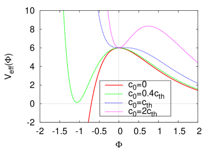
Figure 2: The effective potential $V_{\text{eff}}$ $(p=4$, $q=3)$ of the mode $\Phi$ for various values of fluxes. In the absence of fluxes $c_{0}=0$, the background solution is unstable. For fluxes $0<c_{0}<c_{\text{th}}$ a minimum is formed, to which the system can evolve, and for $c_{0}>c_{\text{th}}$ the background solution is stable.

3.4 Vector Perturbations

The mass spectrum for vector perturbations of the effective $p$-dimensional theory is obtained from the equations of motion for the vector perturbations $b_{\mu n}$ and $V_{\mu n}$. They appear as coefficients in front of the vector harmonics $Y^{I}_{n}(y)$. The system of vector perturbations needs to be diagonalized to find the spectrum and the mass eigenstates. They are linear combinations of the metric vector perturbations $V_{\mu n}$ and the form flux vector perturbations $b_{\mu n}$.

We list the equations of motion for the vector modes obtained from the Einstein and Maxwell equations (18)–(25). The form field is expressed in terms of its gauge potential (3.1). The gauge potential is further decomposed according to the equations (3.1) and the relations (C) are used for simplification

$$\left\{\left[{\hat{\rule{0.0pt}{7.5pt}\Box}\rule{0.0pt}{7.5pt}^{\mu}}_{\,\nu}V_{\mu}+2(p-1)H^{2}V_{\nu}\right]\delta^{m}_{n}+(V_{\mu}+2cb_{\nu})\hat{\Delta}^{m}_{\,\,\,n}\right\}Y_{m} =0\ ,$$ (51)

$$\left\{c^{2}{V^{\lambda}}_{;\lambda}\delta^{m}_{n}-\hat{\Delta}^{m}_{\,\,\,n}c{b^{\lambda}}_{;\lambda}\right\}Y_{m} =0\ ,$$ (52)

$$\left\{\left[-c{\hat{\rule{0.0pt}{7.5pt}\Box}\rule{0.0pt}{7.5pt}^{\mu}}_{\,\nu}b_{\mu}+c^{2}V_{\nu}\right]\delta^{m}_{n}-c\hat{\Delta}^{m}_{\,\,\,n}b_{\nu}\right\}Y_{m} =0\ ,$$ (53)

where ${\hat{\rule{0.0pt}{7.5pt}\Box}\rule{0.0pt}{7.5pt}^{\mu}}_{\,\nu}=\Box\delta^{\,\mu}_{\,\,\nu}-\nabla^{\mu}\nabla_{\nu}$ represents the ordinary Maxwell operator and similarly $\hat{\Delta}^{m}_{\,\,\,n}=\Delta\delta^{m}_{\,\,n}-\nabla^{m}\nabla_{n}$, which up to a sign equals to the action of the Laplace–Beltrami operator $(\text{d}^{\dagger}\text{d}+\text{d}\text{d}^{\dagger})$ on the one-forms $Y_{m}$.

The second equation (52) follows from the third one (53) by differentiation. The two dynamical equations (51) and (53) for the physical vector modes $V_{\mu n}$ and $b_{\mu n}$ can be recast compactly

$${\hat{\rule{0.0pt}{7.5pt}\Box}\rule{0.0pt}{7.5pt}^{\mu}}_{\,\nu}\!\left(\!\begin{array}[]{c}V^{I}_{\mu}\\ cb^{I}_{\mu}\end{array}\!\right)\!Y^{I}_{n}\!=\!\left(\!\begin{array}[c]{c c}\kappa^{I}-2(p-1)H^{2}&2\kappa^{I}\rho^{-2}\\ c^{2}&\kappa^{I}\rho^{-2}\end{array}\!\right)\!\!\left(\!\begin{array}[c]{c}V^{I}_{\nu}\\ cb^{I}_{\nu}\end{array}\!\right)\!Y^{I}_{n},$$ (60)

where $\kappa^{I}$ are the eigenvalues of the Laplace–Beltrami operator, $\rho^{2}\hat{\Delta}^{m}_{\,\,\,n}Y_{m}^{I}(y)=-\kappa^{I}Y_{n}^{I}(y)$, that take values in $(k+1)(q+k-2)$ for $k\geq 1$. The eigenvalues of the mass matrix are given by

$$\rho^{2}m^{2}_{\pm} =\kappa-(q-1)+c^{2}\rho^{2}\pm\sqrt{\left[(q-1)-c^{2}\rho^{2}\right]^{2}+2\kappa c^{2}\rho^{2}}\ ,$$ (61)

$$\frac{m_{\pm}^{2}}{H^{2}} =\frac{\kappa}{q-1}\left[\frac{c^{2}}{H^{2}}+(p-1)\right]-(p-1)\pm\sqrt{(p-1)^{2}+2\kappa\frac{p-1}{q-1}\frac{c^{2}}{H^{2}}+\frac{2\kappa}{q-1}\frac{c^{4}}{H^{4}}}\ ,$$

Like in the case of scalar perturbations, the set of eigenstates $X^{\pm}_{\mu}$ that corresponds to the eigenvalues given in equation (61) consists of a linear combination of the metric perturbations $V_{\mu n}$ and the flux perturbation $b_{\mu n}$:

$$X^{\pm}_{\mu}=V_{\mu}+\frac{\kappa-m^{2}_{\mp}\rho^{2}}{c^{2}\rho^{2}}cb_{\mu}\ ,\hskip 5.0pt\hskip 5.0pt{\hat{\rule{0.0pt}{7.5pt}\Box}\rule{0.0pt}{7.5pt}^{\mu}}_{\,\nu}X^{\pm}_{\mu}=m^{2}_{\pm}X^{\pm}_{\nu}\ ,$$ (62)

where the equations are to be understood for each eigenfunction $Y^{I}_{n}(y)$ separately with corresponding values of $\kappa^{I}$ and $m^{I}_{\pm}$.

It can be shown [19] that the values of $\kappa$ are bound from below by $\kappa\geq 2(q-1)$. The bound is saturated when $Y_{(m|n)}=0$—i.e., for the Killing vectors of the compact space. Together with this bound, it follows immediately from equation (61) that all the mass squares in the spectrum are non-negative. Therefore, de Sitter compactifications are stable with respect to vector modes, or in physical terms, the de Sitter space is stable against the development of anisotropies.

The spectrum consists of two Kaluza–Klein towers, whose scaling depends on two quantities: the size $\rho$ of the extra dimension and the field strength of the flux $c$. It is of interest to investigate the nature of the states with the lowest eigenvalues and the spectrum in the limit of vanishing flux.

In the limit when the form flux is switched off, $c\rightarrow 0$, its perturbation $b_{\mu}$ also vanishes. Only for the negative branch do the coefficients of the mass eigenstates in equation (62) remain regular and the limit can be performed: $X_{\mu n}^{-}\propto V_{\mu n}$. The spectrum (61) reduces to

$$\rho^{2}m^{2}_{-}=\kappa-2(q-1)=\kappa-2(p-1)H^{2}\rho^{2}\ .$$ (63)

The positive branch originates from the presence of the form field fluctuations. It introduces a new scale $c$, but it does not affect the lowest mass modes, which are in either case obtained from the negative branch. One obtains $m_{-}^{2}=0$ for $\kappa=2(q-1)$ and all values of $c$. The lowest vector modes are massless and correspond to the isometries of the compact spacetime. The spectrum of vector modes is summarized in Fig. 4.

In the absence of flux all remaining three parameters of the background model $H$, $\Lambda$ and $\rho$ are related to each other by factors of order unity, cf. equations (7). The flux introduces a new scale and enables us to create a hierarchy between $H$ and the other parameters. When $c$ is very close to its maximal value $c_{\text{max}}$, the number $H\rho^{-1}$ is very small. This creates a hierarchy in a direction that is phenomenologically interesting with $H\ll\rho^{-1}$.

 

Figure 3: The dependence of the mass spectrum for the vector perturbations on the strength of the flux $c$ for $p=4$ and the compact space $S^{3}$.

 

Figure 4: Spectrum of tensor fluctuations for $p=4$ and $S^{3}$.

3.5 Tensor Perturbations

3.5.1 The Homogeneous Graviton.

We show in this subsection that the homogeneous, $y$-independent component of the graviton $h_{(\mu\nu)}$ reduces to the ordinary $p$-dimensional de Sitter graviton. The details about the wave functions and representations can be found in [21].

For the homogeneous mode all $y$-derivatives vanish. Then for the Weyl-shifted metric perturbations $\delta g_{\mu\nu}=h_{\mu\nu}-\frac{2q}{p-2}\Phi\gamma_{\mu\nu}$ and $\delta g_{mn}=(1+2\Phi)g_{mn}$ the left-hand side of the Einstein equations is obtained from equations (16)

$$\delta R^{\text{hom}}_{\mu\nu}=\frac{1}{2}\!\left(h_{\lambda\mu;\nu}^{\hskip 3.5pt\hskip 3.5pt\hskip 3.5pt;\lambda}\!+\!h_{\lambda\nu;\mu}^{\hskip 3.5pt\hskip 3.5pt\hskip 3.5pt;\lambda}\!-\!\Box h_{\mu\nu}\!-\!h^{\lambda}_{\lambda;\mu\nu}\right)\!+\!\frac{q}{p-2}\Box\Phi\gamma_{\mu\nu}\ .$$ (64)

Similarly, the homogeneous contribution of the perturbations to the $(\mu\nu)$-components of the energy–momentum tensor follows from equation (21):

$$\delta S^{\text{hom}}_{\mu\nu}=(p-1)H^{2}h_{\mu\nu}+2q\left(\frac{q-1}{p+q-2}c^{2}-\frac{p-1}{p-2}H^{2}\right)\Phi\gamma_{\mu\nu}\ .$$ (65)

The terms in $\Phi$ of expressions (64) and (65) cancel by virtue of the equations of motion (43) for the zero-mode of $\Phi$. Commuting the derivatives in the expression (64) and imposing transverse and traceless conditions on $h_{\mu\nu}$, equations (64) and (65) reduce to the ordinary equation of motion for the massless graviton in de Sitter space with an apparent mass of $2H^{2}$:

$$\Box h_{\mu\nu}^{\text{TT}}=2H^{2}h_{\mu\nu}^{\text{TT}}\ .$$ (66)

3.5.2 The Inhomogeneous Graviton.

Slightly more involved is the identification of the massive gravitons. The starting point is the traceless component of the $(\mu\nu)$ Einstein equations:

$$0=\frac{1}{2}\left[h_{(\mu\lambda)\hskip 3.5pt;\nu}^{\hskip 3.5pt\hskip 3.5pt\hskip 3.5pt;\lambda}+h_{(\nu\lambda)\hskip 3.5pt;\mu}^{\hskip 3.5pt\hskip 3.5pt\hskip 3.5pt;\lambda}-(\Box+\Delta)h_{(\mu\nu)}\right]\!+H^{2}h_{(\mu\nu)}-\frac{1}{p}h_{(\kappa\lambda)}^{\hskip 3.5pt\hskip 3.5pt\hskip 3.5pt;\kappa\lambda}\gamma_{\mu\nu}-(p-2)\Psi_{;(\mu\nu)}\ .$$ (67)

Next $h_{(\mu\lambda)}^{\hskip 3.5pt\hskip 3.5pt\hskip 3.5pt;\lambda}$, $h_{(\kappa\lambda)}^{\hskip 3.5pt\hskip 3.5pt\hskip 3.5pt;\kappa\lambda}$ and $\Psi$ are eliminated with the scalar equations (28)–(32). One finds

$$\frac{1}{2}\left(\Box+\Delta\right)h_{(\mu\nu)}-H^{2}h_{(\mu\nu)}-2cb_{;(\mu\nu)}=0\ .$$ (68)

The physical graviton is transverse and traceless. Following the ansatz of [16], we construct the physical graviton $\phi_{(\mu\nu)}$ as follows:

$$\phi_{(\mu\nu)}=h_{(\mu\nu)}-(ucb+v\Phi)_{;(\mu\nu)}\ ,$$ (69)

where $u$ and $v$ are arbitrary constants, that are determined from equation (68) and the conditions

$$\Box\phi_{(\mu\nu)} =(-\Delta+2H^{2})\phi_{(\mu\nu)}\ ,$$

$$\phi^{(\mu\lambda)}_{\hskip 3.5pt\hskip 3.5pt\hskip 3.5pt;\lambda} =0\ .$$ (70)

The value of the constants $u$ and $v$ depends on the eigenvalue of the Laplacian $\Delta$ acting on the scalar functions $Y(y)$. They are given by

$$u= \frac{2(p-2)}{(p-1)\left[(p-2)H^{2}-\lambda\rho^{-2}\right]}\ ,$$

$$v= \frac{2(D-2)}{(p-1)\left[\lambda\rho^{-2}-(p-2)H^{2}\right]}\ ,$$ (71)

with the eigenvalues of the Laplacian $\lambda$ that can take values $l(l+q-1)$ for $l\geq 0$. From equation (3.5.2) the spectrum of the graviton is obtained. Neglecting the apparent mass shift of $2H^{2}$ from the de Sitter space, one obtains a simple Kaluza–Klein spectrum for the graviton modes, determined by the geometry of the internal space and unaffected by the bulk matter fields (in our case the form flux $F_{M_{1}\cdots M_{q}}$):

$$\rho^{2}m^{2}_{\text{grav}}=l(l+q-1)\ ,\hskip 5.0pt\hskip 5.0pt\hskip 5.0ptl\geq 0\ .$$ (72)

For comparison, the lowest Kaluza–Klein excitations of the gravitational waves are plotted in Fig. 4.

4 Physical Implications

In this section we analyze two possible consequences for the effective four-dimensional cosmology that result from the properties of the mass spectrum of the scalar, vector and tensor perturbations that we calculated in Sec. 3. (i) During inflation an almost scale invariant spectrum of perturbations is generated for modes whose mass is smaller than the scale of inflation $H$. These perturbations contribute to the later evolution of the universe. (ii) The perturbations gravitationally couple to the standard model fields. We assume that the standard model fields are realized as zero-modes of the corresponding higher dimensional fields and calculate the coupling of the scalar perturbation to the standard model fields.

4.1 The Generation of Perturbations during Inflation

To estimate the dynamics of the perturbations during inflation it is important to know their masses in comparison to the expansion rate $H$. The perturbations are phenomenologically interesting when their mass is smaller than the $H$. Figure 5 shows the mass spectrum of the scalar, vector and tensor perturbations in units of the expansion rate $H$ for a ten-dimensional spacetime compactified on a six-dimensional sphere.

From the spectrum for the scalar perturbations in Fig. 5 we see immediately that, besides the volume modulus, higher Kaluza–Klein excitations can also have masses smaller than the expansion rate $H$ for certain ranges of the form field strength $c$. During inflation an almost scale invariant spectrum of perturbations will be generated for these modes. They therefore contribute as cosmological perturbations to the evolution of the universe. In particular, we note the different nature of the volume modulus and the higher Kaluza–Klein excitations with respect to their coupling to the standard model fields, which is discussed below, cf. Sec. 4.2.

Apart from the massless vector fields that are associated with the Killing vector fields on the $q$-sphere, all vector modes have masses larger than the inflationary scale $H$. Consequently, the Kaluza–Klein modes of vector perturbations are not excited during inflation and should not play an important role in the subsequent cosmological evolution. The massless vector fields are conformal and are not excited during inflation either. Moreover, they will disappear from the spectrum, once compactifications to more realistic internal spaces such as Calabi–Yau manifolds are considered.

Similarly, the Kaluza–Klein excitations of tensor modes have masses above the scale of inflation and do not contribute to the dynamics of cosmological perturbation after inflation. The massless tensor mode corresponds to the ordinary four-dimensional graviton. It carries no information about the extra dimensional nature of the full spacetime. Similar conclusions were derived for braneworld models in [22].

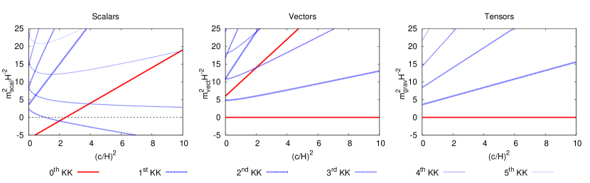
Figure 5: The masses of the scalar, vector and tensor perturbations in units of the expansion rate $H$ of the inflationary geometry for $p=4$ and $q=6$. Unlike the case in Figs. 1–4, there is no limiting flux $c_{\text{max}}$ in this units. The flux $c$ can be arbitrarily larger than the expansions rate $H$.

4.2 The Coupling to Standard Model Fields

Next, we briefly discuss the nature of the coupling of the scalar perturbations to the standard model fields. As a consequence of their different nature, the zero-modes and higher Kaluza–Klein excitations couple differently to the standard model fields. When the standard model fields are localized on a brane, it is known that the radion universally couples to the trace of the energy–momentum tensor of the brane degrees of freedom:

$$S^{\text{brane}}_{\text{int}}=\int d^{4}x\sqrt{\gamma}\Phi T^{\mu}_{\,\mu}\ .$$ (73)

However, in Kaluza–Klein compactifications one does not need to assume that the standard model fields are localized. Instead, the standard model fields of the effective four-dimensional theory simply correspond to the zero-modes of the higher dimensional fields. This point of view modifies the coupling of the volume modulus to the standard model zero-modes and equation (73) is not applicable.

We start with the action (2) and add the standard model Lagrangian as a collection of zero-modes to the full higher dimensional theory:

$$S=\int d^{4}xd^{q}y\sqrt{g_{4+q}}\left\{\frac{1}{2}R-\frac{1}{2q!}F^{2}_{q}-\Lambda+{\cal L}^{\text{zero}}_{\text{SM}}\right\}\ .$$ (74)

For simplicity, we only analyze a canonical scalar field $\chi(x)$:

$${\cal L}^{\text{zero}}_{\text{SM}}=-\frac{1}{2}\left(\partial_{\mu}\chi\right)^{2}-\frac{1}{2}m^{2}\chi^{2}\ .$$ (75)

Focusing on the scalar perturbations $\hat{\Psi}$ and $\Phi$ introduced in the line element (10), the action (74) is expanded to first order:

$$S=\int d^{4}xd^{q}y\sqrt{\gamma}\sqrt{g}\left(1\!+\!4\hat{\Psi}\!+\!q\Phi\right)\left\{\frac{1}{2}(1\!-\!2\hat{\Psi})R[\gamma]+\cdots\right.$$

$$\left.-\frac{1}{2}\left(1\!-\!2\hat{\Psi}\right)(\partial_{\mu}\chi)^{2}-\frac{1}{2}m^{2}\chi^{2}\right\}\ ,$$ (76)

where the dots collect the terms from the form fields, the cosmological constant and the curvature of the internal space. Next the Weyl shift $\hat{\Psi}=\Psi-\frac{q}{2}\Phi$, cf. equation (11), is performed to obtain the linearized Einstein frame and the extra dimensions are integrated out:

$$S_{\text{eff}}=\int d^{4}x\sqrt{\gamma} \left\{\frac{1}{2}\left[1+2\Psi\right]\left[\frac{1}{M_{\text{P}}^{2}}R-\left(\partial_{\mu}\chi\right)^{2}\right]+\cdots-\frac{1}{2}\left(1+4\Psi-q\Phi\right)m^{2}\chi^{2}\right\}\ ,$$ (77)

where the four-dimensional Planck mass $M_{\text{P}}$ arises from the rescaling of the fundamental scale with the volume of the internal space. Similarly the field $\chi$ is rescaled by the volume of the internal space $\sqrt{V_{q}}\chi\rightarrow\chi$. The term $\frac{qm^{2}}{2}\Phi\chi^{2}$ is the reason that the coupling of the volume modulus to the standard model fields deviates from the form in equation (73). Apart from this term the action (77) corresponds to a four-dimensional theory of gravity and a canonical scalar field $\chi$ in a de Sitter geometry with metric fluctuations of the form $ds^{2}=(1+2\Psi)\gamma_{\mu\nu}dx^{\mu}dx^{\nu}$.

We now discuss how the scalar perturbations interact with the standard model fields for the two different cases of a homogeneous (volume modulus) and inhomogeneous Kaluza–Klein excitations.

4.2.1 The Coupling of the Homogeneous Volume Modulus.

The result of the zero-mode for scalar perturbations derived in Sec. 3.3 was particularly simple:

$$\Psi = 0\ ,$$

$$m^{2}_{\Phi} = -6H^{2}+\frac{4(q-1)}{q+2}c^{2}\ .$$ (78)

Therefore, we obtain the effective four-dimensional action for the zero-mode:

$$S_{\text{eff}}=\int d^{4}x\sqrt{\gamma} \left\{\frac{M_{\text{P}}^{2}}{2}R-\frac{1}{2}\left[\left(\partial_{\mu}\chi\right)^{2}+{\cal N}(\partial_{\mu}\Phi)^{2}\right]-\frac{1}{2}(m^{2}\chi^{2}+{\cal N}m^{2}_{\Phi}\Phi^{2})+\frac{qm^{2}}{2M_{\text{P}}}\Phi\chi^{2}\right\}\ ,$$

where $\Phi$ is rescaled to its canonical form up to a constant ${\cal N}$ of order unity. The effective action shows the volume modulus as a canonical scalar field with mass $m_{\Phi}$ that couples to the standard model scalar fields through the interaction term $\Phi\chi^{2}$ and the Planck suppressed coupling $qm^{2}/M_{\text{P}}$. In particular, it has no first-order coupling at all to massless (conformal) fields.

4.2.2 Non-zero Mode Coupling.

Now one can use equation (30) to eliminate $\Psi$. The following four-dimensional interactions are obtained from the effective action (77):

$$S_{\text{int}}\propto\int\!d^{4}x\sqrt{\gamma} \left\{\frac{q-2}{4}\frac{\Phi}{M_{\text{P}}}\left[M^{2}_{\text{P}}R-(\partial_{\mu}\chi)^{2}\right]\!+\!\frac{\Phi}{M_{\text{P}}}m^{2}\chi^{2}\right\}\ .$$ (80)

However, one has to take into account that $\Phi$ is not the physical dynamical variable for the massive modes. The correct kinetic terms and normalizations have to be found for the mass eigenstates calculated in equation (41), which are linear combinations of the scalar perturbation $\Phi$ and the scalar matter degrees of freedom, in our case the scalar component of the form flux $b$. Qualitatively, the interactions in equation (80) show the direct but Planck mass suppressed decay channel of massive Kaluza–Klein states into gravitons and standard model fields. Alternatively, Kaluza–Klein excitations of the scalar perturbation $\Phi$ around its expectation value lead to variations of the Planck mass and the masses of the standard model fields.

5 Conclusions

In this paper, we systematically analyzed the stability properties of de Sitter compactifications with $q$-form fluxes. We calculated in a unified way the complete perturbative mass spectrum of de Sitter compactifications. The most important feature of the perturbative spectrum is the appearance of tachyonic modes in the spectrum of scalar perturbations. The remaining masses of the vector and tensor perturbations of the spectrum are non-negative and therefore do not create additional instabilities.

The tachyonic mode of the volume modulus, possible ways of stabilizing it, and implications for inflation have been discussed before in [11, 12]. Its occurrence imposes tight constraints on the maximal scale of inflation. It also implies that the volume of the internal space is stabilized at least at the scale of inflation to ensure a stable background configuration and a sufficiently large number of efolds during inflation. If the stabilization of the volume modulus remains at such a high scale after inflation, the modulus is too heavy to be detected in future accelerator experiments. The tachyonic nature of the unstabilized modulus is not related to special properties of the internal space. It merely reflects the presence of the inflationary geometry with constant expansion rate $H$ in the effective four-dimensional theory.

Further tachyonic modes that can arise from the quadrupole and higher Kaluza–Klein excitations are less explored. Non-perturbative dynamics that are triggered by these instabilities are not known. A possible stabilization due to additional matter fields is far from obvious, since the instability originates from the presence of the form flux. We therefore expect similar obstructions caused by this instability in more general compactifications.

Figure 6 shows the contour plots for the value of the smallest mass of scalar perturbations as a function of the Hubble scale $H$ and form flux $c$. All quantities are plotted in units of the fundamental mass scale $M=1$. For two or three extra dimensions the lowest mass is by and large determined by the volume modulus, cf. equation (44). For four and more extra dimensions the negative branch in equation (41) of the higher Kaluza–Klein excitations becomes tachyonic for a sufficiently large contribution from the form flux. For four extra dimensions only a small range of parameters $H$ and $c$ admits stable compactifications. For more than four extra dimensions no stable compactifications are found at all in this model. The solid black line in Fig. 6 encircles the region where the size of the extra dimensions $\rho>10M^{-1}$. It is called the SUGRA limit, since for smaller values of $\rho$—i.e., for parameters $H$ and $c$ outside the encircled region—quantum gravity corrections are expected to contribute.

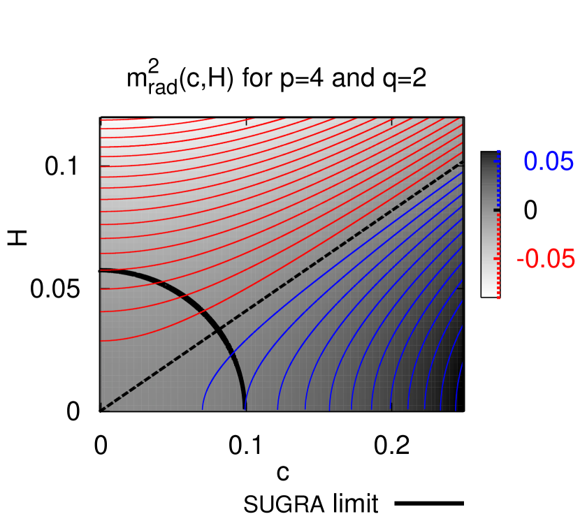
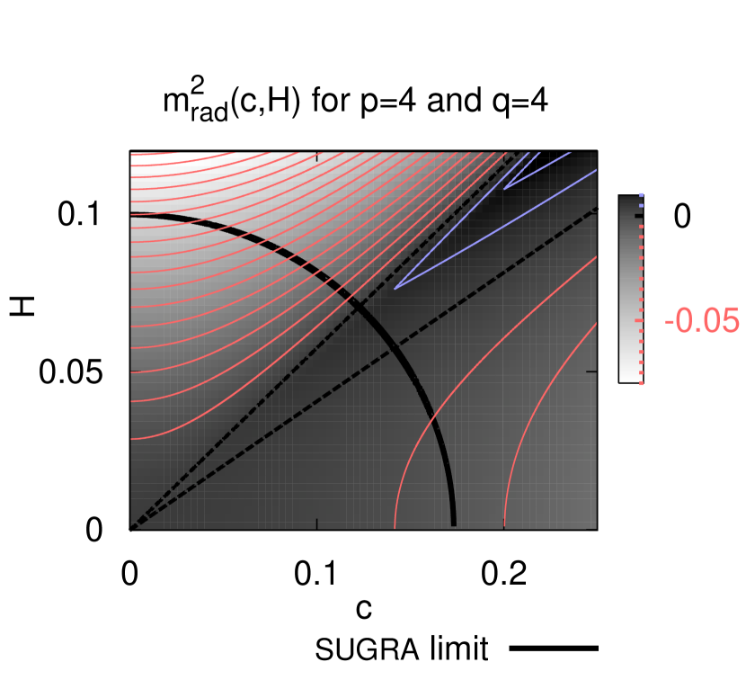
Figure 6: The mass of the lowest lying scalar excitation is shown for two extra dimensions in the left panel and for four extra dimensions in the right panel. The contour lines have a separation of $0.005$ (in fundamental units). The blue (red) contour lines indicate regions of (un)stable compactifications. In the left panel the dashed line represents the parameters for which the mass of the volume modulus vanishes. In the right panel the upper dashed line indicates the zeros for the mass of the volume modulus and the lower dashed line shows where the mass of the second KK mode vanishes. Stable compactifications are only possible for parameters in between the two dashed lines. The solid black line encircles the region in which the size of the extra dimensions is larger than $10$ fundamental units of lengths (i.e., the valid region for the supergravity approximation).

We investigated the calculated spectrum of scalar, vector and tensor perturbations for possible phenomenological consequences. For certain ranges of the form field strength $c$, the scalar sector provides light modes that generate an almost scale-invariant spectrum of fluctuations during inflation. These perturbations decay gravitationally into standard model fields after inflation. The details of the decay are different for the volume modulus and the higher Kaluza–Klein excitations.

The spectrum of vector perturbations (61) does not contain tachyonic modes. Moreover, apart form the massless gauge fields that correspond to the Killing vector fields on the $q$-sphere, all vectors have a mass larger than the scale of inflation, $m_{\text{vec}}>H$ . Furthermore, the vector modes do not have a direct decay channel into standard model fields, since the only conceivable first-order coupling to the standard model fields of the form $V_{(\mu;\nu)}T_{SM}^{\mu\nu}$ can be integrated by parts and vanishes due to the properties of the energy–momentum tensor.

As expected, the spectrum of tensor perturbations does not depend on the details of the matter field content. It only measures the geometry of the compactification. The zero-mode does not feel the presence of the extra dimensions and behaves like an ordinary graviton in the de Sitter geometry. The Kaluza–Klein excitations of the graviton only depend on the size and the shape of the extra dimensions. Again, the massive modes have masses larger than the scale of inflation, $m_{\text{tensor}}>H$. Therefore, Kaluza–Klein excitations of tensor modes will not be generated during inflation. Possible existing excitations from physics before inflation are erased during the process of inflation. Consequently, the massive gravitons are not expected to play a role for cosmological observations.

In the final remark we want to compare this spectrum to the spectrum of anti-de Sitter compactifications calculated in [16]. The main difference in the set up between the two compactifications is the sign in the curvature of the large dimensions and the additional bulk cosmological constant. However, many features do not change qualitatively. Most importantly, the mixing between matter and higher dimensional metric degrees of freedom in the scalar and vector sector is common to both compactifications. It is a well known phenomenon with importance also for the ordinary theory of inflation [23] and braneworld scenarios. The mixing between the higher dimensional metric perturbations and matter fields in braneworlds was investigated in detail in [15]. Even the appearance of modes with negative mass square is common to both supersymmetric and non-supersymmetric compactifications. However, in the case of anti-de Sitter compactifications the stability against perturbations with tachyonic mass is ensured by the Breitenlohner-Freedman bound [24], as long as their mass is larger than this bound.

Appendix A Notation

$x^{M}$	: $(p+q)$-dimensional set of coordinates
$x^{\mu}$	: de Sitter space coordinates
$y^{m}$	: Coordinates of the compact space
$G_{MN}$	: Metric of the full spacetime
$\gamma_{\mu\nu}(x)$	: de Sitter Metric
$g_{mn}(y)$	: Metric of the compact space
$\nabla_{M}\phi$	: Covariant derivative that preserves $G_{M\!N}$
$\nabla_{\mu}\phi\!\equiv\!\phi_{;\mu}$	: Covariant derivative that preserves $\gamma_{\mu\nu}$
$\nabla_{n}\!\phi\!\equiv\!\phi_{|n}$	: Covariant derivative that preserves $g_{mn}$
$Y^{k}(y)$	: Scalar harmonics of the compact space
$Y^{k}_{m}(y)$	: Vector harmonics of the compact space
$Y^{k}_{(mn)}(y)$	: Transverse and traceless harmonics

Appendix B Weyl shift

To understand the redefinition of the scalar perturbation $\hat{\Psi}$ in equation (11), we consider the effective $p$-dimensional theory that is obtained from the compactification of a $(p+q)$-dimensional theory with a choice of metric of the form

$$g_{MN}=\left(\begin{array}[]{c c}\gamma_{\mu\nu}&0\\ 0&e^{2\Phi}g_{mn}\end{array}\right)\ .$$ (81)

For the zero-mode of $\Phi$ and this choice of metric the $(p+q)$-dimensional action of gravity reduces to

$$\int\!d^{p}xd^{q}y\sqrt{|g_{p+q}|}R_{p+q}\!=\!V_{q}\!\int\!d^{p}x\sqrt{|\gamma|}e^{q\Phi}\left[R_{\gamma}\!+\!e^{-2\Phi}R_{g}\right].$$ (82)

To obtain a canonically normalized four dimensional graviton or, in other words, a four-dimensional Einstein theory of gravity, the metric has to be rescaled by a Weyl transformation:

$$\gamma_{\mu\nu}\rightarrow\exp\left({\frac{2q}{p-2}\Phi}\right)\gamma_{\mu\nu}\ .$$ (83)

If the field $\Phi$ is treated as a perturbation as in equation (10), the above Weyl transformation (83) of the metric $\gamma_{\mu\nu}$ amounts to the Weyl shift (11) of the field $\hat{\Psi}$.

Appendix C Form Equations

In this appendix we list useful formulae that have been used to simplify the equations of motion. They are entirely based on the properties of the antisymmetric epsilon tensor and are straightforward to derive:

$$f_{m_{1}\cdots m_{q}}\epsilon^{m_{1}\cdots m_{q}} = q!\,\Delta b\ ,$$

$$f_{mm_{2}\cdots m_{q}}{\epsilon_{n}}^{m_{2}\cdots m_{q}} = (q\!-\!1)!\,\Delta b\,g_{mn}\ ,$$ (84)

$$f_{\mu m_{2}\cdots m_{q}}\epsilon_{n}^{\,\,m_{2}\cdots m_{q}} = (q\!-\!1)!\left(b_{;\mu|n}+{\hat{\Delta}^{l}}_{\,\,n}b_{l\mu}\right).$$

Appendix D Residual Gauge Freedom

As mentioned in Sec. 3.1, the de Donder gauge conditions (12) do not fix the gauge freedom associated with the infinitesimal coordinate transformations (9) completely. Consequently, there will be modes in the spectrum of perturbations that do not correspond to physical degrees of freedom. In this section, we analyze the nature of these residual gauge degrees and impose additional constraints to eliminate them.

The residual gauge freedom consists of functions that satisfy the additional constraints

$$\Delta\xi_{\mu}+{\xi^{l}}_{|l;\mu} = 0\ ,$$

$$\xi_{(m|n)} = 0\ .$$ (85)

There are three distinct solutions that satisfy these constraints:

The $y$-independent infinitesimal diffeomorphisms

$$\xi^{\mu}(x) =\xi^{\mu}_{\perp}(x)+\xi(x)^{;\mu}\ ,$$

$$\xi^{l}(x) \ ,$$ (86)

where we split the $y$-independent diffeomorphisms $\xi^{\mu}(x)$ into a transverse vector $\xi^{\mu}_{\perp}$ and a scalar function $\xi(x)$. Similarly, we decompose the traceless part of homogeneous metric perturbations:

$$h_{(\mu\nu)}(x)=h^{\text{TT}}_{(\mu\nu)}(x)+F^{\perp}_{(\mu;\nu)}(x)+E_{;(\mu\nu)}(x)\ ,$$ (87)

into the transverse-traceless polarizations $h^{\text{TT}}_{(\mu\nu)}$, the transverse vector $F^{\perp}_{\mu}$ and the scalar function $E$. Correspondingly, the homogeneous off-diagonal components of the metric perturbations are decomposed:

$$V_{\mu n}(x)=V^{\perp}_{\mu n}+B_{n;\mu}\ ,$$ (88)

into transverse and longitudinal polarizations.

From the standard transformation of the homogeneous metric perturbations under infinitesimal transformations

$$\delta g_{MN}(x)\rightarrow\delta g_{MN}(x)-\pounds_{\xi}g_{MN}(x)\ ,$$ (89)

with $\pounds_{\xi}$ denoting the Lie derivative in direction of $\xi^{M}$, follows that the additional gauge constraints can be imposed:

$$F^{\perp}_{\mu}=0\ ,\hskip 5.0pt\hskip 5.0pt\hskip 5.0ptE=0\ ,\hskip 5.0pt\hskip 5.0pt\hskip 5.0ptB_{n}=0\ .$$ (90)

These additional constraints ensure that the homogeneous graviton $h_{(\mu\nu)}$ only contains transverse-traceless polarizations and that the homogeneous metric components $V_{\mu n}$ are transverse vectors.

The Killing vectors of the $q$-sphere

$[0,\xi^{l}_{(a)}(y)]$ are another set of solutions $\xi^{M}_{(a)}$, $a=1,\cdots,\frac{1}{2}q(q+1)$ to the equations (D). This gauge symmetry is not removed by further constraints. It remains a symmetry of the effective theory, provided that the massless vector fields $V_{\mu n}$ transform in the adjoint representation of the isometry group of the $q$-sphere, which is generated by the Killing vectors $\xi^{l}_{(a)}$.

The conformal diffeomorphisms

are generated by the scalar harmonics on the $q$-sphere $Y^{I}(y)$ with $l=1$ (i.e., the scalar harmonics that correspond to the first level of Kaluza–Klein excitations). They satisfy the additional constraint $Y_{|(mn)}\equiv Y_{|mn}-\frac{1}{q}g_{mn}\Delta Y=0$. The solution to the equations (D) is given by

$$\xi_{M}=[-k^{I}_{;\mu}(x)Y^{I}(y),k^{I}(x)Y^{I}_{|m}(y)]\ .$$ (91)

This residual symmetry is the reason why the negative branch of the spectrum (41) does not contribute to the physical degrees of freedom of the first excited Kaluza–Klein modes (i.e., $l=1$) [25].

References

- [1] E. . Salam, A. and E. . Sezgin, E., Supergravities in diverse dimensions. Vol. 1, 2. North-Holland, Amsterdam, Netherlands, 1989. 1499 p.
- [2] J. M. Maldacena and C. Nunez, Supergravity description of field theories on curved manifolds and a no go theorem, Int. J. Mod. Phys. A16 (2001) 822–855, [hep-th/0007018].
- [3] S. B. Giddings, S. Kachru, and J. Polchinski, Hierarchies from fluxes in string compactifications, Phys. Rev. D66 (2002) 106006, [hep-th/0105097].
- [4] S. Kachru, R. Kallosh, A. Linde, and S. P. Trivedi, De Sitter vacua in string theory, Phys. Rev. D68 (2003) 046005, [hep-th/0301240].
- [5] L. Cornalba and M. S. Costa, A new cosmological scenario in string theory, Phys. Rev. D66 (2002) 066001, [hep-th/0203031].
- [6] A. R. Frey and A. Mazumdar, 3-form induced potentials, dilaton stabilization, and running moduli, Phys. Rev. D67 (2003) 046006, [hep-th/0210254].
- [7] R. Emparan and J. Garriga, A note on accelerating cosmologies from compactifications and S-branes, JHEP 05 (2003) 028, [hep-th/0304124].
- [8] C.-M. Chen, P.-M. Ho, I. P. Neupane, N. Ohta, and J. E. Wang, Hyperbolic space cosmologies, JHEP 10 (2003) 058, [hep-th/0306291].
- [9] I. P. Neupane, Inflation from string/M-theory compactification?, Nucl. Phys. Proc. Suppl. 129 (2004) 800, [hep-th/0309139].
- [10] N. Ohta, A study of accelerating cosmologies from superstring / M theories, Prog. Theor. Phys. 110 (2003) 269–283, [hep-th/0304172].
- [11] A. V. Frolov and L. Kofman, Can inflating braneworlds be stabilized, Phys. Rev. D69 (2004) 044021, [hep-th/0309002].
- [12] C. R. Contaldi, L. Kofman, and M. Peloso, Gravitational instability of de Sitter compactifications, JCAP 0408 (2004) 007, [hep-th/0403270].
- [13] R. Bousso, O. DeWolfe, and R. C. Myers, Unbounded entropy in spacetimes with positive cosmological constant, Found. Phys. 33 (2003) 297–321, [hep-th/0205080].
- [14] J. Martin, G. N. Felder, A. V. Frolov, M. Peloso, and L. Kofman, Braneworld dynamics with the branecode, Phys. Rev. D69 (2004) 084017, [hep-th/0309001].
- [15] L. Kofman, J. Martin, and M. Peloso, Exact identification of the radion and its coupling to the observable sector, Phys. Rev. D70 (2004) 085015, [hep-ph/0401189].
- [16] H. J. Kim, L. J. Romans, and P. van Nieuwenhuizen, The mass spectrum of chiral supergravity on , Phys. Rev. D32 (1985) 389.
- [17] P. G. O. Freund and M. A. Rubin, Dynamics of dimensional reduction, Phys. Lett. B97 (1980) 233–235.
- [18] T. Han, J. D. Lykken, and R.-J. Zhang, On Kaluza-Klein states from large extra dimensions, Phys. Rev. D59 (1999) 105006, [hep-ph/9811350].
- [19] O. DeWolfe, D. Z. Freedman, S. S. Gubser, G. T. Horowitz, and I. Mitra, Stability of compactifications without supersymmetry, Phys. Rev. D65 (2002) 064033, [hep-th/0105047].
- [20] C. Krishnan, S. Paban, and M. Zanic, Evolution of gravitationally unstable de Sitter compactifications, hep-th/0503025.
- [21] A. Higuchi, Linearized gravity in de Sitter space-time as a representation of , Class. Quant. Grav. 8 (1991) 2005–2021.
- [22] A. V. Frolov and L. Kofman, Gravitational waves from braneworld inflation, hep-th/0209133.
- [23] V. F. Mukhanov, H. A. Feldman, and R. H. Brandenberger, Theory of cosmological perturbations. Part 1. Classical perturbations. Part 2. Quantum theory of perturbations. Part 3. Extensions, Phys. Rept. 215 (1992) 203–333.
- [24] P. Breitenlohner and D. Z. Freedman, Stability in gauged extended supergravity, Ann. Phys. 144 (1982) 249.
- [25] P. van Nieuwenhuizen, The complete mass spectrum of d = 11 supergravity compactified on S(4) and a general mass formula for arbitrary cosets M(4), Class. Quant. Grav. 2 (1985) 1.