hep-th/0412108

QMUL-PH-04-13

Non-Supersymmetric Loop Amplitudes

and MHV Vertices

James Bedford, Andreas Brandhuber, Bill Spence and Gabriele Travaglini ♣♣\clubsuit♣♣\clubsuit$\clubsuit$ {j.a.p.bedford, a.brandhuber, w.j.spence, g.travaglini}@qmul.ac.uk

Department of Physics
Queen Mary, University of London
Mile End Road, London, E1 4NS
United Kingdom

Abstract

We show how the MHV diagram description of Yang-Mills theories can be used to study non-supersymmetric loop amplitudes. In particular, we derive a compact expression for the cut-constructible part of the general one-loop MHV multi-gluon scattering amplitude in pure Yang-Mills theory. We show that in special cases this expression reduces to known amplitudes – the amplitude with adjacent negative-helicity gluons, and the five gluon non-adjacent amplitude. Finally, we briefly discuss the twistor space interpretation of our result.

1 Introduction

Since Witten’s discovery that topological string theory on super twistor space provides a description of ${\cal N}\!=\!4$ super Yang-Mills (SYM) [1], considerable progress has been made using twistor-inspired methods to study Yang-Mills theories. An important factor in this has been the proposal to use maximally helicity violating (MHV) diagrams, built using MHV amplitudes as vertices, in order to derive amplitudes [2]. The MHV diagram construction has the appealing feature that twistor space localisation is built in. The method also carries the great practical advantage of tremendously simplifying the calculation of amplitudes. It was quickly confirmed that MHV diagrams gave correct results at tree level (see [3] for a review of the field up to August 2004). The prognosis at one-loop was initially poor, however, as general arguments indicated that it would be impossible to ignore conformal supergravity fields propagating in the loops [4]. Separately to this, initial explorations of the differential equations satisfied by known one-loop amplitudes appeared to suggest unexpected complications in their twistor-space localisation properties [5].

A direct derivation from MHV diagrams of the one-loop MHV scattering amplitudes in ${\cal N}\!=\!4$ SYM was presented in [6]. The question of the localisation of amplitudes was then revisited, and the complications previously found were seen to be due to the appearance of additional inhomogeneous terms [7] in the differential equations obeyed by one-loop amplitudes. Taking into account the corrections coming from this, one finds that indeed the one-loop MHV amplitudes in ${\cal N}\!=\!4$ SYM localise on pairs of lines in twistor space [8], as the direct construction of [6] suggests. This encourages one to conjecture that the whole quantum theory of ${\cal N}\!=\!4$ SYM possesses simple twistor space localisation properties. By studying the differential equations satisfied by the unitarity cuts of amplitudes, the coefficients of the box functions in the next to MHV (NMHV) amplitudes in ${\cal N}\!=\!4$ SYM have recently been shown to localise on planes in twistor space [9]. A direct MHV diagram construction of these amplitudes has not yet been given however.

The study of the analytic properties of amplitudes, using the twistor-inspired approach, has since been found useful in the general analysis of one-loop amplitudes in ${\cal N}\!=\!4$ Yang-Mills, with a recent derivation of the $(---++++)$ one-loop NMHV amplitude [10, 11]. This coincides with one case of the general one-loop seven-gluon NMHV amplitude which was also found recently [12] using the cut-constructibility approach. For ${\cal N}\!=\!1$ theories, the twistor space structure of one-loop amplitudes was studied in [5, 13, 14] and it was found that the holomorphic anomaly of unitarity cuts [7] leads to differential equations [13], in contrast to algebraic equations for ${\cal N}\!=\!4$ [10], obeyed by the one-loop amplitudes.

MHV diagrams provide a well-defined prescription for the direct derivation of amplitudes. It is natural to ask whether the MHV diagram construction of the one-loop ${\cal N}\!=\!4$ MHV amplitudes of [6] can be generalised in other directions – in particular to theories with less supersymmetry. This has been confirmed in recent work [15, 16], where the MHV diagram method was shown to correctly reproduce the known MHV amplitudes for the ${\cal N}\!=\!1$ chiral multiplet. This result implies that one-loop MHV amplitudes for all supersymmetric gauge theories can be derived from MHV diagrams, and hence have simple localisation properties in twistor space.

The close relationship between the MHV diagram construction and unitarity-based methods [17], first seen in [6], and the success in applying this method to the ${\cal N}\!=\!1$ case, encourages the belief that all cut-constructible amplitudes may be amenable to this new approach. It is also of great importance to explore whether MHV diagrams can be used at loop level in non-supersymmetric theories.111The paper [5] discusses the twistor structure of some non-supersymmetric one-loop amplitudes and the possible role of additional vertices in these models. A recent paper [18] has also developed a generalised MHV diagram construction for scattering amplitudes involving a Higgs boson and gluons. These amplitudes are described in terms of a tree-level, non-supersymmetric effective interaction which arises by integrating out a heavy top quark in one-loop diagrams. These motivations lead one to consider the one-loop MHV amplitudes in pure Yang-Mills theory. These amplitudes consist of terms containing cuts, which we call the cut-constructible part of the amplitude, plus additional rational terms. The amplitudes are of great interest, since they are an example of one-loop $n$-point scattering amplitudes in QCD, where all external particles and the particle running in the loop are gluons, and they can be decomposed as

$${\cal{A}}_{n}^{\textrm{glue}}\ =\ {\cal{A}}_{n}^{{\cal{N}}=4}\,-\,4\,{\cal{A}}_{n}^{{\cal{N}}=1,\,\textrm{chiral}}\,+\,{\cal{A}}_{n}^{\,\textrm{scalar}}\ .$$ (1.1)

The first term describes the contribution of an ${\cal N}\!=\!4$ SYM multiplet to the amplitude. The second is $-4$ times the contribution of an ${\cal N}\!=\!1$ chiral multiplet, and the third is a non-supersymmetric amplitude with only complex scalars propagating in the loop. In this paper we focus on the calculation of the final contribution since the other two are known. A similar supersymmetric decomposition exists for one-loop gluon scattering amplitudes with massless quarks or adjoint fermions running in the loop.

The one-loop MHV amplitude in pure Yang-Mills is known only for two special cases – when the two negative-helicity external gluons are adjacent, the cut-constructible part is known [19]; and, in the five-gluon case, the full amplitude, including rational parts, has been calculated for arbitrary helicity configurations in [20]. In this paper, we will use MHV diagrams to derive a compact expression for the cut-constructible part of the general one-loop MHV multi-gluon amplitude when there are scalar particles in the loop – the last term of (1.1). This generalises the known special cases with adjacent negative-helicity gluons, and the five-gluon non-adjacent amplitude. Moreover, this is the first example of the application of the MHV diagram approach to non-supersymmetric loop amplitudes, and provides further evidence that all cut-constructible (parts of) amplitudes may be derived using standard MHV diagrams. Of course, it would be extremely interesting to extend the MHV diagram method to obtain the rational pieces. This might require the construction of suitable MHV vertices where the off-shell legs are continued to $4-2\epsilon$ dimensions or the inclusion of additional effective vertices as proposed in [5].

The plan for the rest of the paper is as follows. In Section 2 we present the formal expression for the one-loop MHV diagrams with a complex scalar running in the loop, which we use in Section 3 to rederive the known amplitude when the negative-helicity gluons are in adjacent positions. In Section 4 we derive a compact expression for the amplitude in the case where the negative-helicity gluons are in arbitrary positions. Our final result is given by Eq. (4.36). We also briefly comment on the twistor space structure of our result. Section 5 is devoted to some consistency checks of our general amplitude. Specifically, we show that it correctly incorporates the adjacent case result [19], also directly reproduced in Section 3, and the cut-constructible part of the five-gluon amplitude computed in [20]. Finally, we show that our expression has the expected infrared singularities.

For further related work on the string theory side, and on the gauge theory side, see [22]–​​[27] and [28]–​​[34] respectively.

2 The scalar amplitude

In complete similarity with the ${\cal N}\!=\!4$ and ${\cal N}\!=\!1$ cases, see e.g. [15], we can immediately write down the expression for the scalar amplitude in terms of MHV vertices as

$\displaystyle{\cal A}_{n}^{{\rm scalar}}$ $\displaystyle=$ $\displaystyle\sum_{m_{1},m_{2},\pm}\int\!d{\cal M}\ {\cal A}(-l_{1}^{\mp},m_{1},\ldots,i^{-},\ldots,m_{2},l_{2}^{\pm})$ (2.1)
$\displaystyle\qquad\qquad\qquad\!\cdot\,{\cal A}(-l_{2}^{\mp},m_{2}+1,\ldots,j^{-},\ldots,m_{1}-1,l_{1}^{\pm})\ ,$

where the ranges of summation of $m_{1}$ and $m_{2}$ are

$$j+1\leq m_{1}\leq i\ ,\qquad i\leq m_{2}\leq j-1\ .$$ (2.2)

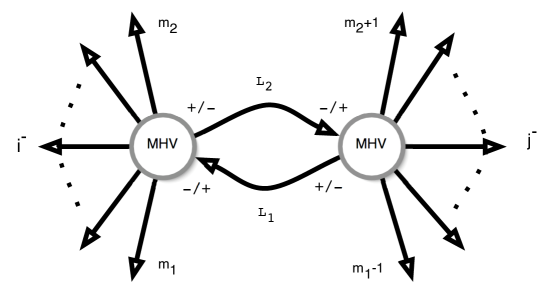
The typical MHV diagram contributing to ${\cal A}_{n}^{{\rm scalar}}$, for fixed $m_{1}$ and $m_{2}$, is depicted in Figure 1.

Refer to caption


Figure 1: A one-loop MHV diagram with a complex scalar running in the loop, computed in Eq. (2.1). We have indicated the possible helicity assignments for the scalar particle.

The off-shell vertices ${\cal A}$ in (2.1) correspond to having complex scalars running in the loop. It follows that there are two possible helicity assignments222For scalar fields, the “helicity” simply distinguishes particles from antiparticles (see, for example, [21]). for the scalar particles in the loop which have to be summed over. These two possibilities are denoted by $\pm$ in (2.1) and in the internal lines in Figure 1. It turns out that each of them gives rise to the same integrand for (2.1),

$$-i{\cal A}_{n}^{\rm tree}\,\cdot\,\frac{\langle m_{2}\,m_{2}\!+\!1\rangle\,\langle m_{1}\!-\!1\,m_{1}\rangle\,\langle i\,l_{1}\rangle^{2}\,\langle j\,l_{1}\rangle^{2}\langle i\,l_{2}\rangle^{2}\langle j\,l_{2}\rangle^{2}}{\langle i\,j\rangle^{4}\,\langle m_{1}\,l_{1}\rangle\,\langle m_{1}\!-\!1\,l_{1}\rangle\,\langle m_{2}\,l_{2}\rangle\,\langle m_{2}\!+\!1\,l_{2}\rangle\,\langle l_{1}\,l_{2}\rangle^{2}}\,\,.$$ (2.3)

A crucial ingredient in (2.1) is the integration measure $d{\cal M}$. This measure was constructed in [6], using the decomposition $L:=l+z\eta$ for a non-null four-vector $L$ in terms of a null vector $l$ and a real parameter $z$. $\eta$ is a null reference vector, which disappears in the final result. We refer the reader to Sections 3 and 4 of [6] for the construction of this measure (also reviewed in Section 3 of [15]), and here we merely quote the result:

$$d{\cal M}\ =\ \frac{dz}{z}\,d^{4-2\epsilon}{\rm LIPS}(l_{2},-l_{1};P_{L;z})\ ,$$ (2.4)

where $L_{i}:=l_{i}+z_{i}\eta$, $i=1,2$ and $z:=z_{1}-z_{2}$. Thus the integration measure $d{\cal M}$ decomposes into the product of a Lorentz-invariant two-particle phase space measure and a dispersive measure $dz/z$. The momentum $P_{L;z}$ flowing in the phase space measure is

$$P_{L;z}\ :=\ P_{L}\,-\,z\eta\ .$$ (2.5)

The interpretation of $dz/z$ as a dispersive measure follows at once when one observes that [6]

$${dz\over z}\ =\ {dP_{L;z}^{2}\over P_{L;z}^{2}-P_{L}^{2}}\ .$$ (2.6)

In order to calculate (2.1), we will first integrate the expression (2.3) over the Lorentz invariant phase space (appropriately regularised to $4-2\epsilon$ dimensions), and then perform the dispersion integral. For the sake of clarity, we will separate the analysis into two parts. Firstly, we will present the (simpler) calculation of the amplitude in the case where the two negative-helicity gluons are adjacent. This particular amplitude has already been computed by Bern, Dixon, Dunbar and Kosower in [19] using the cut-constructibility approach; the result we will derive here will be in precise agreement with the result in that approach. Then, in Section 4 we will move on to address the general case, deriving new results.

3 The scattering amplitude with adjacent negative-helicity gluons

The adjacent case corresponds to choosing $i=m_{1}$, $j=m_{1}-1$ in Figure 1. Therefore we now have a single sum over MHV diagrams, corresponding to the possible choices of $m_{2}$. We will also set $i=2$, $j=1$ for the sake of definiteness, and $m_{2}=m$.

After conversion into traces, the integrand of (2.1) takes on the form:

$\displaystyle\frac{{\mbox{tr}}_{+}(k\!\!\!/_{1}\,k\!\!\!/_{2}\,P\!\!\!\!/_{L;z}\,l\!\!/_{2})\ {\mbox{tr}}_{+}(k\!\!\!/_{1}\,k\!\!\!/_{2}\,l\!\!/_{2}\,P\!\!\!\!/_{L;z})}{2^{5}\,(k_{1}\cdot k_{2})^{3}\,(l_{1}\cdot l_{2})^{2}}\Bigg{\{}\frac{{\mbox{tr}}_{+}(k\!\!\!/_{1}\,k\!\!\!/_{2}\,k\!\!\!/_{m+1}\,l\!\!/_{2})}{(l_{2}\cdot m\!+\!1)}-\frac{{\mbox{tr}}_{+}(k\!\!\!/_{1}\,k\!\!\!/_{2}\,k\!\!\!/_{m}\,l\!\!/_{2})}{(l_{2}\cdot m)}\Bigg{\}}\ ,$ (3.1)

where we note that $(l_{1}\cdot l_{2})=-P_{L;z}^{2}/2$ by momentum conservation.

The next step consists of performing the Passarino-Veltman reduction [35] of the Lorentz invariant phase space integral of (3.1). This requires the calculation of the three-index tensor integral

$${\cal I}^{\mu\nu\rho}(m,P_{L;z})\ =\ \int\!d{\rm LIPS}(l_{2},-l_{1};P_{L;z})\,\frac{l_{2}^{\mu}\,l_{2}^{\nu}\,l_{2}^{\rho}}{(l_{2}\cdot m)}\ .$$ (3.2)

This calculation is performed in Appendix A. The result of this procedure gives the following term at ${\cal O}(\epsilon^{0})$, which we will later integrate with the dispersive measure:

$\displaystyle\tilde{{\cal A}}_{n}^{{\rm scalar}}$ $\displaystyle=$ $\displaystyle\ \frac{\pi}{3}\,(-P_{L;z}^{2})^{-\epsilon}\,\frac{\left[{\mbox{tr}}_{+}(k\!\!\!/_{1}\,k\!\!\!/_{2}\,k\!\!\!/_{m}\,P\!\!\!\!/_{L;z})\right]^{2}}{2^{5}\,(k_{1}\cdot k_{2})^{3}}\,\Bigg{\{}\frac{{\mbox{tr}}_{+}(k\!\!\!/_{1}\,k\!\!\!/_{2}\,P\!\!\!\!/_{L;z}\,k\!\!\!/_{m})}{(m\cdot P_{L;z})^{3}}\ +\ \frac{2(k_{1}\cdot k_{2})}{(m\cdot P_{L;z})^{2}}\Bigg{\}}$
$\displaystyle-$ $\displaystyle\ (m\leftrightarrow m+1)\ ,$ (3.3)

and we have dropped a factor of $4\pi\lambda{\cal A}^{\rm tree}$ on the right hand side of (3.3), where $\lambda$ is defined in (C.1). We can reinstate this factor at the end of the calculation. We also notice that (3.3) is a finite expression, i.e. it is free of infrared poles.

An important remark is in order here. On general grounds, the result of a phase space integral in, say, the $P^{2}$-channel, is of the form

$${\cal I}(\epsilon)\ =\ (-P^{2})^{-\epsilon}\cdot f(\epsilon)\ ,$$ (3.4)

where

$$f(\epsilon)\ =\ {f_{-1}\over\epsilon}\,+\,f_{0}\,+\,f_{1}\epsilon\,+\,\cdots\ ,$$ (3.5)

and $f_{i}$ are rational coefficients. In the case at hand, infrared poles generated by the phase space integrals cancel completely, so that we can in practice replace (3.5) by $f(\epsilon)\to f_{0}\,+\,f_{1}\epsilon\,+\,\cdots$. The amplitude ${\cal A}$ is then obtained by performing a dispersion integral, which converts (3.4) into an expression of the form

$${\cal A}(\epsilon)\ =\ {(-P^{2})^{-\epsilon}\over\epsilon}\cdot g(\epsilon)\ =\ {g_{0}\over\epsilon}\,-\,g_{0}\log(-P^{2})\,+\,g_{1}\,+\,{\cal O}(\epsilon)\ ,$$ (3.6)

where $g(\epsilon)=g_{0}+g_{1}\epsilon+\cdots$, and the coefficients $g_{i}$ are rational functions, i.e. they are free of cuts. Importantly, errors can be generated in the evaluation of phase space integrals if one contracts $(4-2\epsilon)$-dimensional vectors with ordinary four-vectors. This does not affect the evaluation of the coefficient $g_{0}:=g(\epsilon=0)$, and hence the part of the amplitude containing cuts is reliably computed; but the the coefficients $g_{i}$ for $i\geq 1$, in particular $g_{1}$, are in general affected. This implies that rational contributions to the scattering amplitude cannot be detected [19] in this construction. A notable exception to this is provided by the phase space integrals which appear in supersymmetric theories. These are “four-dimensional cut-constructible” [19], in the sense that the rational parts are unambiguously linked to the discontinuities across cuts, and can therefore be uniquely determined.333For more details about cut-constructibility, see the detailed analysis in Sections 3-5 of [19]. This occurs, for example, in the calculation of the ${\cal N}\!=\!4$ MHV amplitudes at one loop performed in [6]. In the present case, however, the relevant phase space integrals violate the cut-constructibility criteria given in [19]444An example of an integral violating the power-counting criterion of [19] is provided by (A.3)., since we encounter tensor triangles with up to three loop momenta in the numerator. Hence, we will be able to compute the part of the amplitude containing cuts, but not the rational terms. In practice, this means that we will compute all phase space integrals up to ${\cal O}(\epsilon^{0})$, and discard ${\cal O}(\epsilon)$ contributions, which would generate rational terms that cannot be determined correctly.

After this digression, we now move on to the dispersion integration. In the center of mass frame, where $P_{L;z}\!:=\!P_{L;z}(1,\textbf{0})$, all the dependence on $P_{L;z}$ in (3.3) cancels out, as there are equal powers of $P_{L;z}$ in the numerator as in the denominator of any term. As a consequence, the dependence on the arbitrary reference vector $\eta$ disappears (see [16] for the application of this argument to the ${\cal N}=1$ case). Using (2.6) in order to re-express $dz/z$ in terms of the relevant dispersive measure, we see that we are left with dispersion integrals of the form

$\displaystyle I(P_{L}^{2})\ :=\ \int\!\frac{ds^{\prime}}{s^{\prime}-P_{L}^{2}}\,(s^{\prime})^{-\epsilon}\ =\ \frac{1}{\epsilon}[\pi\epsilon\csc(\pi\epsilon)]\,(-P_{L}^{2})^{-\epsilon}\ .$ (3.7)

Taking this into account, the dispersion integral of (3.3) then gives

$\displaystyle\!\!\!\tilde{{\cal A}}_{n}^{{\rm scalar}}$ $\displaystyle=$ $\displaystyle\ \big{[}{\pi\epsilon\csc(\pi\epsilon)}\big{]}\,\frac{\pi}{3}\,{(-P_{L}^{2})^{-\epsilon}\over\epsilon}\,\frac{\left[{\mbox{tr}}_{+}(k\!\!\!/_{1}\,k\!\!\!/_{2}\,k\!\!\!/_{m}\,P\!\!\!\!/_{L})\right]^{2}}{2^{5}\,(k_{1}\cdot k_{2})^{3}}\,\Bigg{[}\frac{{\mbox{tr}}_{+}(k\!\!\!/_{1}\,k\!\!\!/_{2}\,P\!\!\!\!/_{L}\,k\!\!\!/_{m})}{(m\cdot P_{L})^{3}}\ +\ \frac{2(k_{1}\cdot k_{2})}{(m\cdot P_{L})^{2}}\Bigg{]}$
$\displaystyle-$ $\displaystyle\ (m\leftrightarrow m+1)\ .$ (3.8)

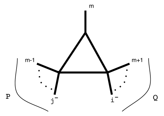
The momentum flow can be conveniently represented as in Figure 2, where we define

$$P\ :=\ q_{2,m-1}\ ,\qquad Q\ :=\ q_{m+1,1}\ =\ -\,q_{2,m}\ ,$$ (3.9)

and $q_{p_{1},p_{2}}:=\sum_{l=p_{1}}^{p_{2}}k_{l}$. We also have $P_{L}:=q_{2,m}=-Q$.

Now we wish to combine the terms in the first line of (3.8) with those in the second line. Since (3.8) is summed over $m$, we simply shift $m+1\to m$ in the terms of the second line. Let us now focus our attention on the second term in (3.3) (similar manipulations will be applied to the first term). Writing the $m\leftrightarrow m+1$ term explicitly, we obtain a contribution proportional to

$$(-P_{L}^{2})^{-\epsilon}\bigg{[}\frac{\left[{\mbox{tr}}_{+}(k\!\!\!/_{1}\,k\!\!\!/_{2}\,k\!\!\!/_{m}\,P\!\!\!\!/_{L})\right]^{2}}{(m\cdot P_{L})^{2}}\ -\ \frac{\left[{\mbox{tr}}_{+}(k\!\!\!/_{1}\,k\!\!\!/_{2}\,k\!\!\!/_{m+1}\,P\!\!\!\!/_{L})\right]^{2}}{((m+1)\cdot P_{L})^{2}}\biggr{]}\ .$$ (3.10)

By shifting $m+1\to m$ in the second term of (3.10), we convert its $P_{L}$ to $P_{L}\to q_{2,m-1}=P$ (whereas, in the non-shifted term, $P_{L}=-Q$). The expression (3.10) then reads

$$\frac{\left[{\mbox{tr}}_{+}(k\!\!\!/_{1}\,k\!\!\!/_{2}\,k\!\!\!/_{m}\,Q\!\!\!\!/)\right]^{2}}{(m\cdot Q)^{2}}\,\Big{[}(-Q^{2})^{-\epsilon}-(-P^{2})^{-\epsilon}\Big{]}\ ,$$ (3.11)

where we used ${\mbox{tr}}_{+}(k\!\!\!/_{1}\,k\!\!\!/_{2}\,k\!\!\!/_{m}Q\!\!\!\!/)=-{\mbox{tr}}_{+}(k\!\!\!/_{1}\,k\!\!\!/_{2}\,k\!\!\!/_{m}P\!\!\!\!/)$ and $Q\cdot m=-P\cdot m$. Notice also that $m\cdot Q=-(1/2)(Q^{2}-P^{2})$.

Refer to caption

Figure 2: A triangle function contributing to the amplitude in the case of adjacent negative helicity gluons. Here we have defined $P:=q_{j,m-1}$, $Q:=q_{m+1,i}=-q_{j,m}$ (in the text we set $i=1$, $j=2$ for definiteness).

Next we re-instate the antisymmetry of the amplitudes under the exchange of the indices $1\leftrightarrow 2$ (which is manifest from equation (2.3)). Doing this we get

$\displaystyle\big{[}{\mbox{tr}}_{+}(k\!\!\!/_{1}\,k\!\!\!/_{2}\,k\!\!\!/_{m}Q\!\!\!\!/)\big{]}^{2}$ $\displaystyle\longrightarrow$ $\displaystyle{1\over 2}\Big{[}\big{(}{\mbox{tr}}_{+}(k\!\!\!/_{1}\,k\!\!\!/_{2}\,k\!\!\!/_{m}\,Q\!\!\!\!/)\big{)}^{2}\,-\,\big{(}{\mbox{tr}}_{+}(k\!\!\!/_{1}\,k\!\!\!/_{2}\,Q\!\!\!\!/\,k\!\!\!/_{m})\big{)}^{2}\Big{]}$
$\displaystyle=$ $\displaystyle 2(k_{1}\cdot k_{2})(m\cdot Q)\Big{[}{\mbox{tr}}_{+}(k\!\!\!/_{1}\,k\!\!\!/_{2}\,k\!\!\!/_{m}\,Q\!\!\!\!/)\,-\,{\mbox{tr}}_{+}(k\!\!\!/_{1}\,k\!\!\!/_{2}\,Q\!\!\!\!/\,k\!\!\!/_{m})\Big{]}\ .$

Following similar steps for the first term in (3.8), we arrive at the following expression for the amplitude before taking the $\epsilon\to 0$ limit:

$${\cal A}_{\epsilon}\ =\ {\cal A}_{1,\epsilon}\,+\,{\cal A}_{2,\epsilon}\ ,$$ (3.13)

where

$\displaystyle{\cal A}_{1,\epsilon}$ $\displaystyle=$ $\displaystyle-{{\cal A}^{\rm tree}\over t_{1}^{[2]}}\cdot{\pi\over 6}\cdot\Bigl{[}{\mbox{tr}}_{+}(k\!\!\!/_{1}\,k\!\!\!/_{2}\,k\!\!\!/_{m}\,q\!\!\!/_{m,1})\,-\,{\mbox{tr}}_{+}(k\!\!\!/_{1}\,k\!\!\!/_{2}\,q\!\!\!/_{m,1}\,k\!\!\!/_{m})\Bigr{]}\,T_{\epsilon}(m,q_{2,m-1},q_{2,m})\ ,$
$\displaystyle{\cal A}_{2,\epsilon}$ $\displaystyle=$ $\displaystyle-{{\cal A}^{\rm tree}\over(t_{1}^{[2]})^{3}}\cdot{\pi\over 3}\cdot\Bigl{[}\big{[}{\mbox{tr}}_{+}(k\!\!\!/_{1}\,k\!\!\!/_{2}\,k\!\!\!/_{m}\,q\!\!\!/_{m,1})\bigl{]}^{2}{\mbox{tr}}_{+}(k\!\!\!/_{1}\,k\!\!\!/_{2}\,q\!\!\!/_{m,1}\,k\!\!\!/_{m})\,-\,$ (3.14)
$\displaystyle-$ $\displaystyle{\mbox{tr}}_{+}(k\!\!\!/_{1}\,k\!\!\!/_{2}\,k\!\!\!/_{m}\,q\!\!\!/_{m,1})\big{[}{\mbox{tr}}_{+}(k\!\!\!/_{1}\,k\!\!\!/_{2}\,q\!\!\!/_{m,1}\,k\!\!\!/_{m})\big{]}^{2}\Bigr{]}\,T_{\epsilon}^{(3)}(m,q_{2,m-1},q_{2,m})\ ,$ (3.15)

and $t_{1}^{[2]}$ follows from the definitions below equation (4.18). In order to write (3.14) in a compact from, we have introduced $\epsilon$-dependent triangle functions [15]

$$T_{\epsilon}^{(r)}(p,P,Q)\ :=\ {1\over\epsilon}{(-P^{2})^{-\epsilon}-(-Q^{2})^{-\epsilon}\over(Q^{2}-P^{2})^{r}}\ ,$$ (3.16)

where $p+P+Q=0$, and $r$ is a positive integer.555For $r=1$ we will omit the superscript $(1)$ in $T^{(1)}$.

We can now take the $\epsilon\to 0$ limit. As long as $P^{2}$ and $Q^{2}$ are non-vanishing, one has

$$\lim_{\epsilon\to 0}T_{\epsilon}^{(r)}(p,P,Q)\ =\ T^{(r)}(p,P,Q)\ ,\qquad P^{2}\neq 0\,,\,Q^{2}\neq 0\ ,$$ (3.17)

where the $\epsilon$-independent triangle functions are defined by

$$T^{(r)}(p,P,Q)\ :=\ {\log(Q^{2}/P^{2})\over(Q^{2}-P^{2})^{r}}\ .$$ (3.18)

If either of the invariants vanishes, the limit of the $\epsilon$-dependent triangle gives rise to an infrared-divergent term (which we call a “degenerate” triangle - this is one with two massless legs). For example, if $Q^{2}=0$, one has

$$\left.T_{\epsilon}(p,P,Q)\right|_{Q^{2}=0}\ \longrightarrow\ -{1\over\epsilon}\,{(-P^{2})^{-\epsilon}\over P^{2}}\,,\qquad{\epsilon\to 0}\ .$$ (3.19)

The two possible configurations which give rise to infrared divergent contributions correspond to the following two possibilities:

  • a.

    $q_{2,m-1}=k_{2}$ (hence $q_{2,m-1}^{2}=0$). In this case we also have $q_{2,m}^{2}=t_{2}^{[2]}$.

  • b.

    $-q_{2,m}=k_{1}$ (hence $q_{2,m}^{2}=0$). Therefore $q_{2,m-1}^{2}=t_{n}^{[2]}$.

We notice that infrared poles will appear only in terms corresponding to the triangle function $T$. Indeed, whenever one of the kinematical invariants contained in $T^{(3)}$ vanishes, the combination of traces multiplying this function in (3.14) vanishes as well.

In conclusion, we arrive at the following result, where we have explicitly separated out the infrared-divergent terms:666A factor of $-4\pi\lambda$ will be understood on the right hand sides of Eqs. (3.20), (3.23), (3.26), where $\lambda$ is defined in (C.1).

$${\cal A}_{n}^{\rm scalar}\ =\ {\cal A}_{\rm poles}\,+\,{\cal A}_{1}\,+\,{\cal A}_{2}\ ,$$ (3.20)

where

$\displaystyle{\cal A}_{\rm poles}$ $\displaystyle=$ $\displaystyle{1\over 6}{\cal A}^{\rm tree}{1\over\epsilon}\Bigl{[}(-t_{2}^{[2]})^{-\epsilon}\,+\,(-t_{n}^{[2]})^{-\epsilon}\Bigr{]}\ ,$ (3.21)
$\displaystyle{\cal A}_{1}$ $\displaystyle=$ $\displaystyle{1\over 6}{\cal A}^{\rm tree}{1\over t_{1}^{[2]}}\,\sum_{m=4}^{n-1}\Bigl{[}{\mbox{tr}}_{+}(k\!\!\!/_{1}\,k\!\!\!/_{2}\,k\!\!\!/_{m}\,q\!\!\!/_{m,1})\,-\,{\mbox{tr}}_{+}(k\!\!\!/_{1}\,k\!\!\!/_{2}\,q\!\!\!/_{m,1}\,k\!\!\!/_{m})\Bigr{]}\,T(m,q_{2,m-1},q_{2,m})\ ,$
$\displaystyle{\cal A}_{2}$ $\displaystyle=$ $\displaystyle{1\over 3}{\cal A}^{\rm tree}{1\over(t_{1}^{[2]})^{3}}\sum_{m=4}^{n-1}\Bigl{[}\big{[}{\mbox{tr}}_{+}(k\!\!\!/_{1}\,k\!\!\!/_{2}\,k\!\!\!/_{m}\,q\!\!\!/_{m,1})\bigl{]}^{2}{\mbox{tr}}_{+}(k\!\!\!/_{1}\,k\!\!\!/_{2}\,q\!\!\!/_{m,1}\,k\!\!\!/_{m})$ (3.22)
$\displaystyle-$ $\displaystyle{\mbox{tr}}_{+}(k\!\!\!/_{1}\,k\!\!\!/_{2}\,k\!\!\!/_{m}\,q\!\!\!/_{m,1})\big{[}{\mbox{tr}}_{+}(k\!\!\!/_{1}\,k\!\!\!/_{2}\,q\!\!\!/_{m,1}\,k\!\!\!/_{m})\big{]}^{2}\Bigr{]}\,T^{(3)}(m,q_{2,m-1},q_{2,m})\ .$

More compactly, we can recognise that ${\cal A}_{\rm poles}$ and ${\cal A}_{1}$ reconstruct the contribution of an ${\cal N}\!=\!1$ chiral supermultiplet, and rewrite (3.20) as

$\displaystyle{\cal A}_{n}^{\textrm{scalar}}\ =\ \frac{1}{3}{\cal A}_{12}^{{\cal N}=1,\,\textrm{chiral}}\ +\ \frac{1}{3}{\cal A}_{12}^{\textrm{tree}}\frac{1}{(t_{1}^{[2]})^{3}}\sum_{m=4}^{n-1}{\cal B}_{12}^{m}\,T^{(3)}(m,q_{2,m-1},q_{2,m})\ ,$ (3.23)

where

$\displaystyle{\cal B}_{12}^{m}$ $\displaystyle=$ $\displaystyle\bigl{[}{\mbox{tr}}_{+}(k\!\!\!/_{1}\,k\!\!\!/_{2}\,k\!\!\!/_{m}\,q\!\!\!/_{m,1})\bigr{]}^{2}{\mbox{tr}}_{+}(k\!\!\!/_{1}\,k\!\!\!/_{2}\,q\!\!\!/_{m,1}\,k\!\!\!/_{m})$ (3.24)
$\displaystyle-$ $\displaystyle\bigl{[}{\mbox{tr}}_{+}(k\!\!\!/_{1}\,k\!\!\!/_{2}\,q\!\!\!/_{m,1}\,k\!\!\!/_{m})\bigr{]}^{2}{\mbox{tr}}_{+}(k\!\!\!/_{1}\,k\!\!\!/_{2}\,k\!\!\!/_{m}\,q\!\!\!/_{m,1})\ .$ (3.25)

and

$${\cal A}_{12}^{{\cal N}=1,\,\textrm{chiral}}\ =\ \frac{1}{2}{\cal A}_{12}^{\textrm{tree}}\frac{1}{t_{1}^{[2]}}\ \sum_{m=3}^{n}\Big{[}{\mbox{tr}}_{+}(k\!\!\!/_{1}\,k\!\!\!/_{2}\,k\!\!\!/_{m}\,q\!\!\!/_{m,1})\,-\,{\mbox{tr}}_{+}(k\!\!\!/_{1}\,k\!\!\!/_{2}\,q\!\!\!/_{m,1}\,k\!\!\!/_{m})\Big{]}\ T(m,q_{2,m-1},q_{2,m})\ .$$ (3.26)

This is our result for the cut-constructible part of the $n$-gluon MHV scattering amplitude with adjacent negative-helicity gluons in positions 1 and 2. This expression was first derived by Bern, Dixon, Dunbar and Kosower in [19], and our result agrees precisely with this. A remark is in order here. In [19], the final result is expressed in terms of a function

$$L_{2}(x)\ :=\ {\log x-(x-1/x)/2\over(1-x)^{3}}\ ,$$ (3.27)

which contains a rational part $-(x-1/x)/2(1-x)^{3}$. This rational part removes a spurious third order pole from the amplitude, but with our approach we did not expect to detect rational terms in the scattering amplitude, and indeed we do not find such terms777In our notation $L_{2}$ corresponds to $T^{(3)}$, which, however, lacks a rational term.. Furthermore, we do not find the other rational terms which are known to be present in the one-loop scattering amplitude [20].

4 The scattering amplitude in the general case

The situation where the negative-helicity gluons are not adjacent is technically more challenging. Our starting point will be (2.3), to which we will apply the Schouten identity (see Appendix D for a collection of spinor identities used in this paper). Eq. (2.3) can then be written as a sum of four terms:888We drop the factor of $-i{\cal A}_{n}^{\rm tree}$ from now on and reinstate it at the end of the calculation.

$\displaystyle{\cal C}(m_{1},m_{2}+1)\ -\ {\cal C}(m_{1},m_{2})\ -\ {\cal C}(m_{1}-1,m_{2}+1)\ +\ {\cal C}(m_{1}-1,m_{2})\ ,$ (4.1)

where

$\displaystyle{\cal C}(a,b)\ :=\ \frac{\langle i\,l_{1}\rangle\,\langle j\,l_{1}\rangle^{2}\,\langle i\,l_{2}\rangle^{2}\,\langle j\,l_{2}\rangle}{\langle i\,j\rangle^{4}\,\langle l_{1}\,l_{2}\rangle^{2}}\,\cdot\,\frac{\langle i\,a\rangle\,\langle j\,b\rangle}{\langle l_{1}\,a\rangle\,\langle l_{2}\,b\rangle}\ .$ (4.2)

The calculation of the phase space integral of this expression is discussed in Appendix B. The result is

$\displaystyle\!\!\!\!\!\!\!\!\!\!\!\!\!\!\!\!\!\!\!\!\!\!\!\!\int\!d^{4-2\epsilon}{\rm LIPS}(l_{2},-l_{1};P_{L;z})\ \ {\cal C}(a,b)$
$\displaystyle\quad=\ \frac{1}{3}\ \frac{{\mbox{tr}}_{+}(i\!\!\!/\,j\!\!\!/\,{b/}\,a\!\!\!/)}{(a\cdot b)}\ \Bigg{[}{\mbox{tr}}_{+}(i\!\!\!/\,j\!\!\!/\,P\!\!\!\!/_{L;z}\,a\!\!\!/)^{2}\bigg{[}\frac{{\mbox{tr}}_{+}(i\!\!\!/\,j\!\!\!/\,a\!\!\!/\,P\!\!\!\!/_{L;z})}{(P_{L;z}\cdot a)^{3}}+\frac{2(i\cdot j)}{(P_{L;z}\cdot a)^{2}}\bigg{]}-(a\leftrightarrow b)\Bigg{]}$ (4.3)
$\displaystyle\quad\qquad+\ \frac{1}{2}\ \frac{{\mbox{tr}}_{+}(i\!\!\!/\,j\!\!\!/\,{b/}\,a\!\!\!/){\mbox{tr}}_{+}(i\!\!\!/\,j\!\!\!/\,a\!\!\!/\,{b/})}{(a\cdot b)^{2}}\ \Bigg{[}\frac{{\mbox{tr}}_{+}(i\!\!\!/\,j\!\!\!/\,P\!\!\!\!/_{L;z}\,a\!\!\!/)^{2}}{(P_{L;z}\cdot a)^{2}}+(a\leftrightarrow b)\Bigg{]}$ (4.4)
$\displaystyle\qquad\qquad-\ \frac{{\mbox{tr}}_{+}(i\!\!\!/\,j\!\!\!/\,a\!\!\!/\,{b/}){\mbox{tr}}_{+}(i\!\!\!/\,j\!\!\!/\,{b/}\,a\!\!\!/)}{(a\cdot b)^{3}}\ \Bigg{[}\frac{{\mbox{tr}}_{+}(i\!\!\!/\,j\!\!\!/\,a\!\!\!/\,{b/}){\mbox{tr}}_{+}(i\!\!\!/\,j\!\!\!/\,P\!\!\!\!/_{L;z}\,a\!\!\!/)}{(P_{L;z}\cdot a)}+(a\leftrightarrow b)\Bigg{]}$ (4.5)
(4.6)
$\displaystyle\qquad\qquad\qquad+\ \frac{{\mbox{tr}}_{+}(i\!\!\!/\,j\!\!\!/\,a\!\!\!/\,{b/})^{2}{\mbox{tr}}_{+}(i\!\!\!/\,j\!\!\!/\,{b/}\,a\!\!\!/)^{2}}{(a\cdot b)^{4}}\ \log\bigg{(}1-\frac{(a\cdot b)}{N}P_{L;z}^{2}\bigg{)}\ ,$ (4.7)

where $N:=N(P):=(a\cdot b)P^{2}-2(P\cdot a)(P\cdot b)$, and we have suppressed a factor of $-4\pi\lambda(-P_{L}^{2})^{-\epsilon}\cdot[2^{8}(i\cdot j)^{4}]^{-1}$ on the right hand side of (4), where $\lambda$ is defined in (C.1). We notice that (4) is symmetric under the simultaneous exchange of $i$ with $j$ and $a$ with $b$. This symmetry is manifest in the coefficient multiplying the logarithm – the last term in (4); for the remaining terms, nontrivial gamma matrix identities are required. For instance, consider the terms in the second line of (4). These terms are present in the adjacent gluon case (3.3), and it is therefore natural to expect that the trace structure of this term is separately invariant when $i\leftrightarrow j$ and $a\leftrightarrow b$. Indeed this is the case, thanks to the identity

$\displaystyle 32(i\cdot j)^{3}$ $\displaystyle=$ $\displaystyle{\mbox{tr}}_{+}(i\!\!\!/\,j\!\!\!/\,P\!\!\!\!/_{L;z}\,a\!\!\!/)^{2}\bigg{[}\frac{{\mbox{tr}}_{+}(i\!\!\!/\,j\!\!\!/\,a\!\!\!/\,P\!\!\!\!/_{L;z})}{(P_{L;z}\cdot a)^{3}}\,+\,\frac{2(i\cdot j)}{(P_{L;z}\cdot a)^{2}}\bigg{]}$
$\displaystyle+$ $\displaystyle{\mbox{tr}}_{+}(i\!\!\!/\,j\!\!\!/\,a\!\!\!/\,P\!\!\!\!/_{L;z})^{2}\bigg{[}\frac{{\mbox{tr}}_{+}(i\!\!\!/\,j\!\!\!/\,P\!\!\!\!/_{L;z}\,a\!\!\!/)}{(P_{L;z}\cdot a)^{3}}\,+\,\frac{2(i\cdot j)}{(P_{L;z}\cdot a)^{2}}\bigg{]}\ .$

Similar identities show that the third and fourth line of (4) are invariant under the simultaneous exchange $i\leftrightarrow j$ and $a\leftrightarrow b$.

The next step is to perform the dispersion integral of (4), i.e. the integral over the variable $z$. This appears in the terms involving $P_{L;z}$ in (4), and in an overall factor $(P_{L;z}^{2})^{-\epsilon}$ arising from the dimensionally regulated measure.

The integral over the term involving the logarithm has been evaluated in [6], with the result

$\displaystyle\int\frac{dz}{z}(P_{L;z}^{2})^{-\epsilon}\log\left(1-\frac{(a\cdot b)}{N}P_{L;z}^{2}\right)$ $\displaystyle=$ $\displaystyle\int\frac{dP_{L;z}^{2}}{P_{L;z}^{2}-P_{L}^{2}}(P_{L;z}^{2})^{-\epsilon}\log\bigg{(}1-\frac{(a\cdot b)}{N}P_{L;z}^{2}\bigg{)}$ (4.10)
$\displaystyle=$ $\displaystyle{\rm Li}_{2}\left(1-\frac{(a\cdot b)}{N(P)}P_{L}^{2}\right)\ +\ {\cal O}(\epsilon)\ .$

Notice that these terms were not present in the adjacent negative-gluon case considered in Section 3.

Next we move on to the remaining terms in (4). Inspecting their $z$-dependence, we see that, in complete similarity with the adjacent case of Section 3, in each term there are the same powers of $P_{L;z}$ in the numerator as in the denominator. Hence, in the centre of mass frame in which $P_{L;z}\!:=\!P_{L;z}(1,\textbf{0})$, one finds that $P_{L;z}$ cancels completely. Note that this also immediately resolves the question of gauge invariance for these terms – this occurs only through the $\eta$ dependence in $P_{L;z}=P_{L}-z\eta$. Furthermore, the box functions coming from (4.10) are separately gauge invariant [6]. The conclusion is that our expression for the amplitude below, built from sums over MHV diagrams of the dispersion integral of (4), will be gauge invariant. Moreover, apart from (4.10), the only other dispersion integral we will need is that computed in (3.7).

It follows from this discussion that the result of the dispersion integral of (4) is (suppressing a factor of $-4\pi\lambda(-P_{L}^{2})^{-\epsilon}\cdot[2^{8}(i\cdot j)^{4}]^{-1}\cdot[\pi\epsilon\csc(\pi\epsilon)]$):

$\displaystyle\!\!\!\!\!\!\!\!\int\frac{dz}{z}\,\int\!d^{4-2\epsilon}{\rm LIPS}(l_{2},-l_{1};P_{L;z})\ \ {\cal C}(a,b)$
$\displaystyle\quad=\ \ \frac{1}{\epsilon}\ {(-P_{L}^{2})^{-\epsilon}}\ \Bigg{\{}\ \frac{1}{3}\ \frac{{\mbox{tr}}_{+}(i\!\!\!/\,j\!\!\!/\,{b/}\,a\!\!\!/)}{(a\cdot b)}\ \Bigg{[}{\mbox{tr}}_{+}(i\!\!\!/\,j\!\!\!/\,P\!\!\!\!/_{L}\,a\!\!\!/)^{2}\bigg{[}\frac{{\mbox{tr}}_{+}(i\!\!\!/\,j\!\!\!/\,a\!\!\!/\,P\!\!\!\!/_{L})}{(P_{L}\cdot a)^{3}}+\frac{2(i\cdot j)}{(P_{L}\cdot a)^{2}}\bigg{]}-(a\leftrightarrow b)\Bigg{]}$ (4.11)
$\displaystyle\quad\qquad+\ \frac{1}{2}\ \frac{{\mbox{tr}}_{+}(i\!\!\!/\,j\!\!\!/\,{b/}\,a\!\!\!/){\mbox{tr}}_{+}(i\!\!\!/\,j\!\!\!/\,a\!\!\!/\,{b/})}{(a\cdot b)^{2}}\ \Bigg{[}\frac{{\mbox{tr}}_{+}(i\!\!\!/\,j\!\!\!/\,P\!\!\!\!/_{L}\,a\!\!\!/)^{2}}{(P_{L}\cdot a)^{2}}+(a\leftrightarrow b)\Bigg{]}$ (4.12)
$\displaystyle\qquad\qquad-\ \frac{{\mbox{tr}}_{+}(i\!\!\!/\,j\!\!\!/\,a\!\!\!/\,{b/}){\mbox{tr}}_{+}(i\!\!\!/\,j\!\!\!/\,{b/}\,a\!\!\!/)}{(a\cdot b)^{3}}\ \Bigg{[}\frac{{\mbox{tr}}_{+}(i\!\!\!/\,j\!\!\!/\,a\!\!\!/\,{b/}){\mbox{tr}}_{+}(i\!\!\!/\,j\!\!\!/\,P\!\!\!\!/_{L}\,a\!\!\!/)}{(P_{L}\cdot a)}+(a\leftrightarrow b)\Bigg{]}\ \Bigg{\}}$ (4.13)
(4.14)
$\displaystyle\qquad\qquad\qquad+\ \frac{{\mbox{tr}}_{+}(i\!\!\!/\,j\!\!\!/\,a\!\!\!/\,{b/})^{2}{\mbox{tr}}_{+}(i\!\!\!/\,j\!\!\!/\,{b/}\,a\!\!\!/)^{2}}{(a\cdot b)^{4}}\ {\rm Li}_{2}\left(1-\frac{(a\cdot b)}{N(P_{L})}P_{L}^{2}\right)\ .$ (4.15)

Now, due to the four terms in (4.1), the sum over MHV diagrams will include a signed sum over four expressions like (4). Let us begin by considering the last line of (4). This is a term familiar from [6] and [15], corresponding to one of the four dilogarithms in the novel expression found in [6] for the finite part $B$ of a scalar box function,

$\displaystyle B(s,t,P^{2},Q^{2})$ $\displaystyle=$ $\displaystyle{\rm Li}_{2}\left(1-\frac{(a\cdot b)}{N(P)}P^{2}\right)\,+\,{\rm Li}_{2}\left(1-\frac{(a\cdot b)}{N(P)}Q^{2}\right)$ (4.17)
$\displaystyle-$ $\displaystyle{\rm Li}_{2}\left(1-\frac{(a\cdot b)}{N(P)}s\right)\,-\,{\rm Li}_{2}\left(1-\frac{(a\cdot b)}{N(P)}t\right)\ ,$

with $s:=(P+a)^{2}$, $t:=(P+b)^{2}$, and $P+Q+a+b=0$. By taking into account the four terms in (4.1) and summing over MHV diagrams as specified in (2.1) and (2.2), one sees that each of the four terms in any finite box function $B$ appears exactly once, in complete similarity with [6] and [15], so that the final contribution of this term will be999We multiply our final results by a factor of $2$, which takes into account the two possible helicity assignments for the scalars in the loop.

$$\sum_{m_{1}=j+1}^{i-1}\sum_{m_{2}=i+1}^{j-1}{1\over 2}\,\big{[}b_{m_{1}m_{2}}^{ij}\big{]}^{2}\,B(q_{m_{1},m_{2}-1}^{2},q_{m_{1}+1,m_{2}}^{2},q_{m_{1}+1,m_{2}-1}^{2},q_{m_{2}+1,m_{1}-1}^{2})\ ,$$ (4.18)

where $t_{i}^{[k]}:=(p_{i}+p_{i+1}+\cdots+p_{i+k-1})^{2}$ for $k\geq 0$, and $t_{i}^{[k]}=t_{i}^{[n-k]}$ for $k<0$. In writing (4.18), we have taken into account that the dilogarithm in (4) is multiplied by a coefficient proportional to the square of $b_{m_{1}m_{2}}^{ij}$, where

$$b_{m_{1}m_{2}}^{ij}\ :=\ -2\,\frac{\mbox{tr}_{+}\left(k\!\!\!/_{i}k\!\!\!/_{j}k\!\!\!/_{m_{1}}k\!\!\!/_{m_{2}}\right)\mbox{tr}_{+}\left(k\!\!\!/_{i}k\!\!\!/_{j}k\!\!\!/_{m_{2}}k\!\!\!/_{m_{1}}\right)}{[(k_{i}+k_{j})^{2}]^{2}\,[(k_{m_{1}}+k_{m_{2}})^{2}]^{2}}\ .$$ (4.19)

We notice that $b_{m_{1}m_{2}}^{ij}$ is the coefficient of the box functions in the one-loop ${\cal N}\!=\!1$ MHV amplitude, originally calculated by Bern, Dixon, Dunbar and Kosower in [19], and derived in [15, 16] using the MHV diagram approach for loops proposed in [6].

Refer to caption

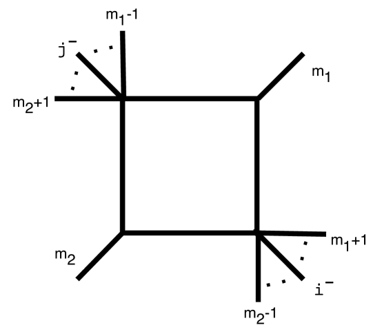
Figure 3: A box function contributing to the amplitude in the general case. The negative-helicity gluons, $i$ and $j$, cannot be in adjacent positions, as the figure shows.

Furthermore, we observe that $b_{m_{1}m_{2}}^{ij}$ is holomorphic in the spinor variables, and as such has simple localisation properties in twistor space. Indeed, from (4.19) it follows that

$$b_{m_{1}m_{2}}^{ij}\ =\ 2\,{\langle i\,m_{1}\rangle\,\langle i\,m_{2}\rangle\,\langle j\,m_{1}\rangle\,\langle j\,m_{2}\rangle\over\langle i\,j\rangle^{2}\,\langle m_{1}\,m_{2}\rangle^{2}}\ .$$ (4.20)

Summing over the four terms for the remainder of (4) can be done in complete similarity with Section 4 of [15].101010In Section 3 we have illustrated in detail how this sum is performed for the simpler case of adjacent negative-helicity gluons. We will skip the details of this derivation, and will now present our result.

In order to do this, we find it convenient to define the following expressions:

$\displaystyle A^{ij}_{m_{1}m_{2}}$ $\displaystyle:=$ $\displaystyle{(i\,j\,m_{2}+1\,m_{1})\over((m_{2}+1)\cdot m_{1})}\,-\,{(i\,j\,m_{2}\,m_{1})\over(m_{2}\cdot m_{1})}$
$\displaystyle=$ $\displaystyle-2\,[i\,j]\,\langle m_{1}\,i\rangle\langle m_{1}\,j\rangle\,{\langle m_{2}\,m_{2}+1\rangle\over\langle m_{2}+1\,m_{1}\rangle\,\langle m_{1}\,m_{2}\rangle}\ ,$
$\displaystyle S^{ij}_{m_{1}m_{2}}$ $\displaystyle:=$ $\displaystyle{(i\,j\,m_{1}\,m_{2}+1)(i\,j\,m_{2}+1\,m_{1})\over((m_{2}+1)\cdot m_{1})^{2}}\,-\,{(i\,j\,m_{1}\,m_{2})(i\,j\,m_{2}\,m_{1})\over(m_{2}\cdot m_{1})^{2}}\ ,$ (4.23)
$\displaystyle I^{ij}_{m_{1}m_{2}}$ $\displaystyle:=$ $\displaystyle{(i\,j\,m_{1}\,m_{2}+1)^{2}(i\,j\,m_{2}+1\,m_{1})\over((m_{2}+1)\cdot m_{1})^{3}}\,-\,{(i\,j\,m_{1}\,m_{2})^{2}(i\,j\,m_{2}\,m_{1})\over(m_{2}\cdot m_{1})^{3}}\ ,$ (4.24)

where for notational simplicity we set $(a_{1}\,a_{2}\,a_{3}\,a_{4}):={\mbox{tr}}_{+}(a\!\!\!/_{1}a\!\!\!/_{2}a\!\!\!/_{3}a\!\!\!/_{4})$ in the above. We also note the symmetry properties

$$A^{ji}_{m_{1}m_{2}}\,=\,-A^{ij}_{m_{1}m_{2}}\ ,\qquad S^{ji}_{m_{1}m_{2}}\,=\,S^{ij}_{m_{1}m_{2}}\ .$$ (4.25)

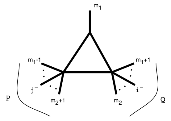
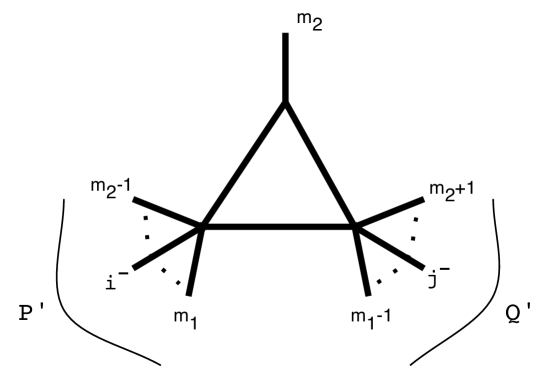
The momentum flow is best described using the triangle diagram in Figure 4, where we use the following definitions:

$\displaystyle P$ $\displaystyle:=$ $\displaystyle q_{m_{2}+1,m_{1}-1}\ =\ -q_{m_{1},m_{2}}\ ,$ (4.26)
$\displaystyle Q$ $\displaystyle:=$ $\displaystyle q_{m_{1}+1,m_{2}}\ .$

The triangle in Figure 5 also appears in the calculation, and can be converted into a triangle as in Figure 4 – but with $i$ and $j$ swapped – if one shifts $m_{1}-1\to m_{1}$, and then swaps $m_{1}\leftrightarrow m_{2}$.

We then introduce the coefficients

$\displaystyle{\cal A}^{ij}_{m_{1}m_{2}}$ $\displaystyle:=$ $\displaystyle 2^{-8}(i\cdot j)^{-4}\,A^{ij}_{m_{1}m_{2}}\,\Big{[}(i\,j\,m_{1}\,Q)^{2}(i\,j\,Q\,m_{1})\,-\,(i\,j\,m_{1}\,Q)(i\,j\,Q\,m_{1})^{2}\Big{]},$ (4.27)
$\displaystyle\tilde{{\cal A}}^{ij}_{m_{1}m_{2}}$ $\displaystyle:=$ $\displaystyle 2^{-8}(i\cdot j)^{-4}\,A^{ij}_{m_{1}m_{2}}\,\Big{[}(i\,j\,m_{1}\,Q)^{2}\,-\,(i\,j\,Q\,m_{1})^{2}\Big{]}\,,$ (4.29)
$\displaystyle{\cal S}^{ij}_{m_{1}m_{2}}$ $\displaystyle=$ $\displaystyle 2^{-8}{(i\cdot j)^{-4}}\,S^{ij}_{m_{1}m_{2}}\,\Big{[}(i\,j\,m_{1}\,Q)^{2}\,+\,(i\,j\,Q\,m_{1})^{2}\Big{]}\ ,$ (4.31)
$\displaystyle{\cal I}^{ij}_{m_{1}m_{2}}$ $\displaystyle:=$ $\displaystyle 2^{-8}(i\cdot j)^{-4}\,\Big{[}I^{ij}_{m_{1}m_{2}}\,(i\,j\,Q\,m_{1})\,+\,I^{ji}_{m_{1}m_{2}}(i\,j\,m_{1}\,Q)\Big{]}\ .$ (4.33)

We will also make use of the $\epsilon$-dependent triangle functions introduced in (3.16), whose $\epsilon\to 0$ limits have been considered in (3.17)–(3.19). This is in order to write a compact expression which incorporates also the infrared-divergent terms.111111The infrared-divergent terms will be described below, and used to check that our result has the correct infrared pole structure.

We can now present our result for the one-loop MHV amplitude (2.1)121212We thank Lance Dixon for pointing out some typos, both in these equations and elsewhere, in an earlier version of the paper.:

$\displaystyle{\cal A}_{\rm scalar}$ $\displaystyle=$ $\displaystyle{\cal A}_{\rm tree}\bigg{\{}\sum_{m_{1}=j+1}^{i-1}\sum_{m_{2}=i+1}^{j-1}{1\over 2}\big{[}b_{m_{1}m_{2}}^{ij}\big{]}^{2}\,B(q_{m_{1},m_{2}-1}^{2},q_{m_{1}+1,m_{2}}^{2},q_{m_{1}+1,m_{2}-1}^{2},q_{m_{2}+1,m_{1}-1}^{2})$ (4.34)
$\displaystyle-$ $\displaystyle\bigg{(}\,{8\over 3}\sum_{m_{1}=j+1}^{i-1}\sum_{m_{2}=i}^{j-1}\Big{[}{\cal A}_{m_{1}m_{2}}^{ij}\,T^{(3)}(m_{1},P,Q)\,-\,(i\cdot j)\tilde{{\cal A}}^{ij}_{m_{1}m_{2}}\,T^{(2)}(m_{1},P,Q)\Big{]}$
$\displaystyle+$ $\displaystyle 2\sum_{m_{1}=j+1}^{i-1}\sum_{m_{2}=i}^{j-1}\Big{[}{\cal S}^{ij}_{m_{1}m_{2}}\,T^{(2)}(m_{1},P,Q)\,+\,{\cal I}^{ij}_{m_{1}m_{2}}\,T(m_{1},P,Q)\Big{]}$
$\displaystyle\qquad+\ (i\longleftrightarrow j)\ \ \biggr{)}\ \biggr{\}}\ ,$

where on the right hand side of (4.34) a factor of $-4\pi\lambda$ is understood, where $\lambda$ is defined in (C.1). We can also introduce the coefficient

$$c_{m_{1}m_{2}}^{ij}\ :=\ {1\over 2}\bigg{[}{(i\,j\,m_{2}+1\,m_{1})\over\big{(}(m_{2}+1)\cdot m_{1}\big{)}}\,-\,{(i\,j\,m_{2}\,m_{1})\over(m_{2}\cdot m_{1})}\bigg{]}\,{(i\,j\,m_{1}\,Q)\,-\,(i\,j\,Q\,m_{1})\over[(i\,+\,j)^{2}]^{2}}\ ,$$ (4.35)

which already appears as the coefficient multiplying the triangle function $T$ in the ${\cal N}\!=\!1$ amplitude, (see e.g. Eq. (2.19) of [15]), and rewrite (4.34) as

$\displaystyle{\cal A}_{\rm scalar}$ $\displaystyle=$ $\displaystyle{\cal A}_{\rm tree}\bigg{\{}\sum_{m_{1}=j+1}^{i-1}\sum_{m_{2}=i+1}^{j-1}{1\over 2}\big{[}b_{m_{1}m_{2}}^{ij}\big{]}^{2}\,B(q_{m_{1},m_{2}-1}^{2},q_{m_{1}+1,m_{2}}^{2},q_{m_{1}+1,m_{2}-1}^{2},q_{m_{2}+1,m_{1}-1}^{2})$ (4.36)
$\displaystyle-$ $\displaystyle\bigg{(}\,{1\over 2}\sum_{m_{1}=j+1}^{i-1}\sum_{m_{2}=i}^{j-1}{1\over 3}\,c^{ij}_{m_{1}m_{2}}\,\Big{[}{(i\,j\,m_{1}\,Q)\,(i\,j\,Q\,m_{1})\over 2(i\cdot j)^{2}}\,T^{(3)}(m_{1},P,Q)\,+\,\,T(m_{1},P,Q)\Big{]}$
$\displaystyle+$ $\displaystyle 2\sum_{m_{1}=j+1}^{i-1}\sum_{m_{2}=i}^{j-1}\Big{[}{\cal S}^{ij}_{m_{1}m_{2}}\,T^{(2)}(m_{1},P,Q)\,+\,{\cal I}^{ij}_{m_{1}m_{2}}\,T(m_{1},P,Q)\Big{]}$
$\displaystyle\qquad+\ (i\longleftrightarrow j)\ \ \biggr{)}\ \biggr{\}}\ .$

Refer to caption

Figure 4: One type of triangle function contributing to the amplitude in the general case, where $i\in Q$, and $j\in P$.

Refer to caption

Figure 5: Another type of triangle function contributing to the amplitude in the general case. By first shifting $m_{1}-1\to m_{1}$, and then swapping $m_{1}\leftrightarrow m_{2}$, we convert this into a triangle function as in Figure 5 – but with $i$ and $j$ swapped. These are the triangle functions responsible for the $i\leftrightarrow j$ swapped terms in (4.34) – or (4.36).

Several remarks are in order.

  • 1.

    As usual, the variables $q_{m_{1},m_{2}-1}^{2}$, $q_{m_{1}+1,m_{2}}^{2}$ correspond to the $s$- and $t$-channel of the finite part of the “easy two-mass” box function with massless legs $m_{1}$ and $m_{2}$, and massive legs $q_{m_{1}+1,m_{2}-1}^{2}$, $q_{m_{2}+1,m_{1}-1}^{2}$ (Figure 3).

  • 2.

    Compared to the range for $m_{1}$ and $m_{2}$ indicated in (2.2), we have omitted $m_{1}=i$ in the summation of the triangles, as for this value the coefficients $A$, $S$, $I$ defined in (4.27)–(4.33) vanish. Notice also that we have $i\in Q$ and $j\in P$.

  • 3.

    In the case of adjacent negative-helicity gluons, the only surviving terms are those containing the coefficient $c^{ij}_{m_{1}m_{2}}$, on the second line of (4.34) or (4.36). We will return to this point in Section 5.

  • 4.

    We comment that, in contrast to the adjacent case (see (3.23)), in the general case the ${\cal N}=1$ chiral amplitude does not separate out naturally in the final result, as one can see from the coefficient of the box function $B$ in (4.34).

Next we wish to separate explicitly the infrared divergences from (4.34). We can immediately anticipate that there will be four infrared-divergent terms, corresponding to the four possible degenerate triangles. Two of these degenerate triangles occur when either $P^{2}$ or $Q^{2}$ happen to vanish. The other two originate from the $i\leftrightarrow j$ swapped terms.

Let us consider first the terms arising from the summation with $i\leftrightarrow j$ unswapped. When $Q^{2}=0$, it follows that $m_{1}=i-1$ and $m_{2}=i$ (see Figure 4). When $P^{2}=0$, it follows that $m_{1}=j+1$ and $m_{2}=j-1$ (see Figure 5). Hence

$\displaystyle T^{(r)}(p,P,Q)$ $\displaystyle\to$ $\displaystyle(-)^{r}\,{1\over\epsilon}\,{(-t_{i-1}^{[2]})^{-\epsilon}\over(t_{i-1}^{[2]})^{r}}\ ,\qquad Q^{2}\to 0\ ,$ (4.37)
$\displaystyle T^{(r)}(p,P,Q)$ $\displaystyle\to$ $\displaystyle-\,{1\over\epsilon}\,{(-t_{j}^{[2]})^{-\epsilon}\over(t_{j}^{[2]})^{r}}\ ,\qquad\quad\ \ P^{2}\to 0\ .$

The infrared-divergent terms coming from $Q^{2}=0$ are then easily extracted, and are

$\displaystyle-{1\over 2\epsilon}$ $\displaystyle\cdot$ $\displaystyle(-t_{i-1}^{[2]})^{-\epsilon}\,4(i\cdot j)\,{(i\,j\,i-1\,i+1)\over\big{(}(i+1)\cdot(i-1)\big{)}}$
$\displaystyle\cdot$ $\displaystyle\bigg{[}{8\over 3}(i\cdot j)^{2}\,-\,2\,{(i\,j\,i+1\,i-1)\over\big{(}(i+1)\cdot(i-1)\big{)}}(i\cdot j)\,+\,{(i\,j\,i+1\,i-1)(i\,j\,i-1\,i+1)\over\big{(}(i+1)\cdot(i-1)\big{)}^{2}}\bigg{]}\ ,$

and from $P^{2}=0$

$\displaystyle-{1\over 2\epsilon}$ $\displaystyle\cdot$ $\displaystyle(-t_{j}^{[2]})^{-\epsilon}\,4(i\cdot j)\,{(i\,j\,j-1\,j+1)\over\big{(}(j+1)\cdot(j-1)\big{)}}$
$\displaystyle\cdot$ $\displaystyle\bigg{[}{8\over 3}(i\cdot j)^{2}\,-\,2\,{(i\,j\,j+1\,j-1)\over\big{(}(j+1)\cdot(j-1)\big{)}}(i\cdot j)\,+\,{(i\,j\,j+1\,j-1)(i\,j\,j-1\,j+1)\over\big{(}(j+1)\cdot(j-1)\big{)}^{2}}\bigg{]}\ .$

Likewise, from the “swapped” degenerate triangles we obtain the following infrared-divergent terms:

$\displaystyle-{1\over 2\epsilon}$ $\displaystyle\cdot$ $\displaystyle(-t_{j-1}^{[2]})^{-\epsilon}\,4(i\cdot j)\,{(i\,j\,j+1\,j-1)\over\big{(}(j+1)\cdot(j-1)\big{)}}$
$\displaystyle\cdot$ $\displaystyle\bigg{[}{8\over 3}(i\cdot j)^{2}\,-\,2\,{(i\,j\,j-1\,j+1)\over\big{(}(j+1)\cdot(j-1)\big{)}}(i\cdot j)\,+\,{(i\,j\,j-1\,j+1)(i\,j\,j+1\,j-1)\over\big{(}(j+1)\cdot(j-1)\big{)}^{2}}\bigg{]}\ ,$

and

$\displaystyle-{1\over 2\epsilon}$ $\displaystyle\cdot$ $\displaystyle(-t_{i}^{[2]})^{-\epsilon}\,4(i\cdot j)\,{(i\,j\,i+1\,i-1)\over\big{(}(i+1)\cdot(i-1)\big{)}}$
$\displaystyle\cdot$ $\displaystyle\bigg{[}{8\over 3}(i\cdot j)^{2}\,-\,2\,{(i\,j\,i-1\,i+1)\over\big{(}(i+1)\cdot(i-1)\big{)}}(i\cdot j)\,+\,{(i\,j\,i-1\,i+1)(i\,j\,i+1\,i-1)\over\big{(}(i+1)\cdot(i-1)\big{)}^{2}}\bigg{]}\ .$

4.1 Comments on twistor space interpretation

We would like to make some brief comments on the interpretation in twistor space of our result (4.36).

  • 1.

    As noticed earlier, the coefficient $b^{ij}_{m_{1}m_{2}}$ appears already in the ${\cal N}\!=\!1$ chiral supermultiplet contribution to a one-loop MHV amplitude, where it multiplies the box function. It was noticed in Section 4 of [5] that $b^{ij}_{m_{1}m_{2}}$ is a holomorphic function, hence it does not affect the twistor space localisation of the finite box function.131313We thank Dave Dunbar for discussions on this point.

  • 2.

    The coefficient $c^{ij}_{m_{1}m_{2}}$ also appears in the ${\cal N}\!=\!1$ amplitude, as the coefficient of the triangles (see e.g.  Eq. (2.19) of [15]). Its twistor space interpretation was considered in Section 4 of [5], where it was found that $c^{ij}_{m_{1}m_{2}}$ has support on two lines in twistor space. Furthermore, it was also found that the corresponding term in the amplitude has a derivative of a delta function support on coplanar configurations.

  • 3.

    The combination $c^{ij}_{m_{1}m_{2}}\,(i\,j\,m_{1}\,Q)\,(i\,j\,Q\,m_{1})/(i\cdot j)^{2}$ already appears in the case of adjacent negative-helicity gluons. The localisation properties of the corresponding term in the amplitude were considered in Section 5.3 of [5], and found to have, similarly to the previous case, derivative of a delta function support on coplanar configurations.

  • 4.

    On general grounds, we can argue that the remaining terms in the amplitude have a twistor space interpretation which is similar to that of the terms already considered. The gluons whose momenta sum to $P$ are contained on a line; likewise, the gluons whose momenta sum to $Q$ localise on another line.

We observe that the rational parts of the amplitude are not generated from the MHV diagram construction presented here. Such rational terms were not present for the ${\cal N}=1$ and ${\cal N}=4$ amplitudes derived in [6, 15, 16]. However, for the amplitude studied here, rational terms are required to ensure correct factorisation properties [19].

5 Checks of the general result

In this Section we present three consistency checks that we have performed for the result (4.34) (or (4.36)) for the one-loop scalar contribution to the MHV scattering amplitude. These checks are:

  • 1.

    For adjacent negative-helicity gluons, the general expression (4.34) should reproduce the previously calculated form (3.23).

  • 2.

    In the case of five gluons in the configuration $(1^{-}2^{+}3^{-}4^{+}5^{+})$, the result (4.34) should reproduce the known amplitude given in [20].

  • 3.

    The result (4.34) should have the correct infrared-pole structure.

We next discuss these requirements in turn.

5.1 Adjacent case

The amplitude where the two negative-helicity external gluons are adjacent is given in Section 7 of [19] and was explicitly rederived in Section 3 of this paper by combining MHV vertices, see Eq. (3.23). It is easy to show that our general result (4.36) reproduce correctly (3.23) as a special case.

To start with, recall that our result (4.36) is expressed in terms of box-functions and triangle functions, see Figure 3 and Figures 4, 5 respectively. In the adjacent case, the box functions are not present. Indeed, in the sum (4.18) the negative-helicity gluons can never be in adjacent positions (see Figure 3).

Next, we focus on the triangles of Figure 4. In terms of these triangles, requiring $i$ and $j$ to be adjacent eliminates the sum over $m_{2}$, as we must have $m_{2}=i$ and $m_{2}+1=j$. Moreover, in this case $Q=q_{m_{1}+1,i}$, $P=q_{j,m_{1}-1}$ and one has

$\displaystyle A_{ij}^{m_{1}m_{2}}$ $\displaystyle=$ $\displaystyle-4\,(i\cdot j)\ ,$
$\displaystyle S_{ij}^{m_{1}m_{2}}$ $\displaystyle=$ $\displaystyle 0\ ,\qquad I_{ij}^{m_{1}m_{2}}\ =\ 0\ ,$ (5.2)

for $m_{2}=i$, and $m_{2}+1=j$. Similar simplifications occur for the swapped triangle. Hence the only surviving terms are those in the second line of (4.34) (or (4.36)), and it is then easy to see that they generate the same amplitude (3.8) already calculated in Section 3.

5.2 Five-gluon amplitude

The other special case is the non-adjacent five-gluon amplitude $(1^{-}2^{+}3^{-}4^{+}5^{+})$, given in Eq. (9) of [20]. This amplitude may be written as $c_{\Gamma}{\cal A}_{\rm tree}$ times141414The derivation in [20] used string-based methods, which affects the coefficient of the pole term. In (5.2) we have written the pole coefficient which matches the adjacent case.

$\displaystyle\frac{1}{6\epsilon}-\frac{1}{6}\log(-s_{34})\ +\ \frac{{\mbox{tr}}_{+}(1\!\!\!/\,3\!\!\!/\,2\!\!\!/\,5\!\!\!/)^{2}\ {\mbox{tr}}_{+}(1\!\!\!/\,3\!\!\!/\,5\!\!\!/\,2\!\!\!/)^{2}}{2^{7}(2\cdot 5)^{4}(1\cdot 3)^{4}}\ B(s_{51},s_{12},0,s_{34})$
$\displaystyle-\ \frac{1}{3}\ \frac{{\mbox{tr}}_{+}(1\!\!\!/\,3\!\!\!/\,2\!\!\!/\,5\!\!\!/)\ {\mbox{tr}}_{+}(1\!\!\!/\,3\!\!\!/\,5\!\!\!/\,2\!\!\!/)}{2^{4}(2\cdot 5)(1\cdot 3)^{4}}\ \left[\ {\mbox{tr}}_{+}(1\!\!\!/\,3\!\!\!/\,5\!\!\!/\,2\!\!\!/)^{2}\ \frac{\log(s_{12}/s_{34})}{(s_{12}-s_{34})^{3}}+{\mbox{tr}}_{+}(1\!\!\!/\,3\!\!\!/\,2\!\!\!/\,5\!\!\!/)^{2}\ \frac{\log(s_{34}/s_{51})}{(s_{34}-s_{51})^{3}}\ \right]$ (5.3)
$\displaystyle+\ \frac{1}{3}\ \frac{1}{2^{3}(1\cdot 3)^{3}}\left[\ {\mbox{tr}}_{+}(1\!\!\!/\,3\!\!\!/\,4\!\!\!/\,2\!\!\!/){\mbox{tr}}_{+}(1\!\!\!/\,3\!\!\!/\,2\!\!\!/\,5\!\!\!/)^{2}\ \frac{\log(s_{34}/s_{51})}{(s_{34}-s_{51})^{3}}\ \right]$ (5.4)
$\displaystyle-\ \frac{{\mbox{tr}}_{+}(1\!\!\!/\,3\!\!\!/\,2\!\!\!/\,5\!\!\!/)^{2}\ {\mbox{tr}}_{+}(1\!\!\!/\,3\!\!\!/\,5\!\!\!/\,2\!\!\!/)^{2}}{2^{6}(2\cdot 5)^{2}(1\cdot 3)^{4}}\left[\ \ \frac{\log(s_{12}/s_{34})}{(s_{12}-s_{34})^{2}}-\frac{\log(s_{34}/s_{51})}{(s_{34}-s_{51})^{2}}\ \right]$ (5.5)
$\displaystyle+\ \frac{{\mbox{tr}}_{+}(1\!\!\!/\,3\!\!\!/\,2\!\!\!/\,5\!\!\!/)^{2}\ {\mbox{tr}}_{+}(1\!\!\!/\,3\!\!\!/\,5\!\!\!/\,2\!\!\!/)^{2}}{2^{6}(2\cdot 5)^{3}(1\cdot 3)^{4}}\left[\ \frac{\log(s_{12}/s_{34})}{(s_{12}-s_{34})}+\frac{\log(s_{34}/s_{51})}{(s_{34}-s_{51})}\ \right]$ (5.6)
$\displaystyle-\ \frac{1}{3}\ \frac{1}{2^{2}(1\cdot 3)}\left[\ {\mbox{tr}}_{+}(1\!\!\!/\,3\!\!\!/\,2\!\!\!/\,5\!\!\!/)\ \frac{\log(s_{34}/s_{51})}{(s_{34}-s_{51})}\ \right]$ (5.7)
(5.8)
$\displaystyle\quad+\quad(1,4)\leftrightarrow(3,5)\ \ ,$ (5.9)

where the interchange on the last line applies to all terms above it in this equation, including the first two terms, and the box function $B$ is defined in (4.17). In deriving this from [20], we have used the dilogarithm identity

$\displaystyle\!\!\!\!\!\!\!\!\!\!\!\!{\rm Li}_{2}(1-r)+{\rm Li}_{2}(1-s)+\log(r)\log(s)\ ={\rm Li}_{2}\bigg{(}\frac{1-r}{s}\bigg{)}+{\rm Li}_{2}\bigg{(}\frac{1-s}{r}\bigg{)}-{\rm Li}_{2}\bigg{(}\frac{1-s}{r}\frac{1-r}{s}\bigg{)}.$
(5.10)

We have checked explicitly that our expression for the $n$-gluon non-adjacent amplitude (4.34), when specialised to the case with five gluons in the configuration $(1^{-}2^{+}3^{-}4^{+}5^{+})$, yields precisely the result (5.2) above. For the terms involving dilogarithms, this is easily done. For the remaining terms, which contain logarithms, a more involved calculation is necessary using various spinor identities from Appendix D. A straightforward method of doing this calculation begins with the explicit sum over MHV diagrams in this case, isolating the coefficients of each logarithmic function such as e.g. $\log(s_{12})$, and then checking that these coefficients match those in (5.2). The remaining $1/\epsilon$ term arises from the following discussion.

5.3 Infrared-pole structure

The infrared-divergent terms (poles in $1/\epsilon$) can easily be extracted from (4)–(4) by simply replacing $(-t_{r}^{[2]})^{-\epsilon}\to 1$ ($r=i-1,i,j-1,j$). Consider first the terms in (4) and (4). After a little algebra, and using

$$(i\,j\,j+1\,j-1)\,+\,(i\,j\,j-1\,i-1)\ =\ 4\,(i\cdot j)\,\big{(}(j-1)\cdot(j+1)\big{)}\ ,$$ (5.12)

one finds that these two contributions add up to

$$-{64\over 3\,\epsilon}\ (i\cdot j)^{4}\ .$$ (5.13)

Similarly, the pole contribution arising from (4) and (4) gives an additional contribution of $-({64/3\,\epsilon})\ (i\cdot j)^{4}$. Reinstating a factor of $-2\cdot 2^{-8}(i\cdot j)^{-4}\cdot{\cal A}_{\rm tree}$, we see that the pole part of (4.34) is simply given by

$$\left.{\cal A}_{\rm scalar}\right|_{\rm\epsilon-pole}\ =\ {{\cal A}_{\rm tree}\over 3}\ .$$ (5.14)

Hence our result (4.34) has the expected infrared-singular behaviour.

Acknowledgements

It is a pleasure to thank Lance Dixon, Dave Dunbar, Michael Green, Marek Karliner, Valya Khoze, David Kosower, Marco Matone and Sanjaye Ramgoolam for discussions. GT acknowledges the support of PPARC.

Appendix A: Passarino-Veltman reduction

In Section 2 we saw that a typical term in the cut-constructible part of the Yang-Mills amplitude is the dispersion integral of the following phase space integral:

$\displaystyle{\cal C}(m)\,:=\,\int\!d{\rm LIPS}(l_{2},-l_{1};P_{L;z})\,\frac{{\mbox{tr}}_{+}(k\!\!\!/_{1}\,k\!\!\!/_{2}\,P\!\!\!\!/_{L;z}\,l\!\!/_{2})\,{\mbox{tr}}_{+}(k\!\!\!/_{1}\,k\!\!\!/_{2}\,l\!\!/_{2}\,P\!\!\!\!/_{L;z})\,{\mbox{tr}}_{+}(k\!\!\!/_{1}\,k\!\!\!/_{2}\,k\!\!\!/_{m}\,l\!\!/_{2})}{(l_{2}\cdot m)\,(k_{1}\cdot k_{2})^{3}\,(P_{L;z}^{2})^{2}}\,.$ (A.1)

The goal of this Appendix is to perform the Passarino-Veltman reduction [35] of (A.1). To this end, we rewrite ${\cal C}(m)$ as

$${\cal C}(m)\ =\ {{\mbox{tr}}_{+}(k\!\!\!/_{1}\,k\!\!\!/_{2}\,P\!\!\!\!/_{L;z}\,\gamma_{\mu})\ {\mbox{tr}}_{+}(k\!\!\!/_{1}\,k\!\!\!/_{2}\,\gamma_{\nu}\,P\!\!\!\!/_{L;z})\ {\mbox{tr}}_{+}(k\!\!\!/_{1}\,k\!\!\!/_{2}\,k\!\!\!/_{m}\,\gamma_{\rho})\over(k_{1}\cdot k_{2})^{3}(P_{L;z}^{2})^{2}\,}\ {\cal I}^{\mu\nu\rho}(m,P_{L;z})\ ,$$ (A.2)

where151515For the rest of this Appendix we drop the subscript $z$ in $P_{L;z}$ for the sake of brevity.

$${\cal I}^{\mu\nu\rho}(m,P_{L})\ =\ \int\!d{\rm LIPS}(l_{2},-l_{1};P_{L})\,\frac{l_{2}^{\mu}\,l_{2}^{\nu}\,l_{2}^{\rho}}{(l_{2}\cdot m)}\ .$$ (A.3)

On general grounds, ${\cal I}^{\mu\nu\rho}(m,P_{L})$ can be decomposed as

$\displaystyle{\cal I}^{\mu\nu\rho}$ $\displaystyle=$ $\displaystyle m^{\mu}m^{\nu}m^{\rho}\,{\cal I}_{1}\ +\ (m^{\mu}m^{\nu}P_{L}^{\rho}\,+\,m^{\mu}P_{L}^{\nu}m^{\rho}\,+\,P_{L}^{\mu}m^{\nu}m^{\rho})\,{\cal I}_{2}$ (A.6)
$\displaystyle+$ $\displaystyle(m^{\mu}P_{L}^{\nu}P_{L}^{\rho}\,+\,P_{L}^{\mu}m^{\nu}P_{L}^{\rho}+P_{L}^{\mu}P_{L}^{\nu}m^{\rho})\,{\cal I}_{3}\ +\ P_{L}^{\mu}P_{L}^{\nu}P_{L}^{\rho}\,{\cal I}_{4}$
$\displaystyle+$ $\displaystyle(\eta^{\mu\nu}m^{\rho}\,+\,\eta^{\mu\rho}m^{\nu}\,+\,\eta^{\nu\rho}m^{\mu})\,{\cal I}_{5}\ +\ (\eta^{\mu\nu}P_{L}^{\rho}\,+\,\eta^{\mu\rho}P_{L}^{\nu}\,+\,\eta^{\nu\rho}P_{L}^{\mu}){\cal I}_{6}\ ,$

for some coefficients ${\cal I}_{i},i=0,...,6$. One can then contract with different combinations of the independent momenta in order to solve for the ${\cal I}_{i}$. Introducing the quantities

$\displaystyle A$ $\displaystyle:=$ $\displaystyle\ m_{\mu}m_{\nu}m_{\rho}\,I^{\mu\nu\rho}\ ,$ (A.7)
$\displaystyle B$ $\displaystyle:=$ $\displaystyle\ m_{\mu}m_{\nu}P_{L\rho}\,I^{\mu\nu\rho}\ ,$ (A.8)
$\displaystyle C$ $\displaystyle:=$ $\displaystyle\ m_{\mu}P_{L\nu}P_{L\rho}\,I^{\mu\nu\rho}\ ,$ (A.9)
$\displaystyle D$ $\displaystyle:=$ $\displaystyle\ P_{L\mu}P_{L\nu}P_{L\rho}\,I^{\mu\nu\rho}\ ,$ (A.10)
$\displaystyle E$ $\displaystyle:=$ $\displaystyle\ \eta_{\mu\nu}m_{\rho}\,I^{\mu\nu\rho}\ \ =\ 0\ ,$ (A.11)
$\displaystyle F$ $\displaystyle:=$ $\displaystyle\ \eta_{\mu\nu}P_{L\rho}\,I^{\mu\nu\rho}\ =\ 0\ ,$ (A.12)

the result for the Passarino-Veltman reduction of $\{{\cal I}_{1},\ldots,{\cal I}_{6}\}$ in the basis $\{A,\ldots,D\}$ is:

$\displaystyle{\cal I}_{2}$ $\displaystyle=$ $\displaystyle\left(5(P_{L}^{2})^{2}/\big{(}2(m\cdot P_{L})^{5}\big{)}\,,\,-6P_{L}^{2}/(m\cdot P_{L})^{4}\,,\,3/(m\cdot P_{L})^{3}\,,\,0\right)\ ,$ (A.13)
$\displaystyle{\cal I}_{3}$ $\displaystyle=$ $\displaystyle\left(-2P_{L}^{2}/(m\cdot P_{L})^{4}\,,\,3/(m\cdot P_{L})^{3}\,,\,0\,,\,0\right)\ ,$ (A.14)
$\displaystyle{\cal I}_{4}$ $\displaystyle=$ $\displaystyle\left(1/(m\cdot P_{L})^{3}\,,\,0\,,\,0\,,\,0\right)$ (A.15)
$\displaystyle{\cal I}_{5}$ $\displaystyle=$ $\displaystyle\left(-(P_{L}^{2})^{2}/\big{(}2(m\cdot P_{L})^{4}\big{)}\,,3P_{L}^{2}/\big{(}2(m\cdot P_{L})^{3}\big{)}\,,\,-1/(m\cdot P_{L})^{2}\,,\,0\right)\ ,$ (A.16)
$\displaystyle{\cal I}_{6}$ $\displaystyle=$ $\displaystyle\left(P_{L}^{2}/\big{(}2(m\cdot P_{L})^{3})\,,-1/(m\cdot P_{L})^{2}\,,0\,,0\right)\ .$ (A.17)

We omit the decomposition for ${\cal I}_{1}$, as the corresponding term in (A.6) drops out of all future expressions due to $k_{m}^{2}=0$.

Finally, using the methods of [15] and the results of Appendix C, the integrals in (A.7) are found to be, keeping only terms to order $\mathcal{O}(\epsilon^{0})$,

$\displaystyle A$ $\displaystyle=$ $\displaystyle\ (m\cdot P_{L})^{2}\,{4\over 3}\pi\lambda\ ,$ (A.18)
$\displaystyle B$ $\displaystyle=$ $\displaystyle\ P_{L}^{2}(m\cdot P_{L})\,\pi\lambda\,,$ (A.20)
$\displaystyle C$ $\displaystyle=$ $\displaystyle\ (P_{L}^{2})^{2}\,\pi\lambda\,,$ (A.22)
$\displaystyle D$ $\displaystyle=$ $\displaystyle\ -\frac{(P_{L}^{2})^{3}}{8(m\cdot P_{L})}\,\frac{4\pi}{\epsilon}\,\lambda\,,$ (A.24)

where

$$\lambda\ :=\frac{\pi^{\frac{1}{2}-\epsilon}}{4^{1-\epsilon}\,\Gamma\big{(}\frac{1}{2}-\epsilon\big{)}}\ .$$ (A.25)

Appendix B: Evaluating the integral of ${\cal C}(a,b)$

The basic expression which arises in the MHV diagram construction in this paper is

$\displaystyle{\cal C}(a,b)=\frac{\langle i\,l_{1}\rangle\,\langle j\,l_{1}\rangle^{2}\,\langle i\,l_{2}\rangle^{2}\,\langle j\,l_{2}\rangle}{\langle i\,j\rangle^{4}\,\langle l_{1}\,l_{2}\rangle^{2}}\frac{\langle i\,a\rangle\,\langle j\,b\rangle}{\langle l_{1}\,a\rangle\,\langle l_{2}\,b\rangle}.$ (B.1)

We wish to integrate this expression over the Lorentz invariant phase space. We begin by simplifying it, using multiple applications of the Schouten identity. First note that using this identity twice, one deduces that

$\displaystyle\frac{\langle i\,l_{2}\rangle\,\langle j\,l_{1}\rangle}{\langle l_{1}\,a\rangle\,\langle l_{2}\,b\rangle}\langle a\,b\rangle^{2}$ $\displaystyle=$ $\displaystyle\langle i\,a\rangle\langle b\,j\rangle+\langle i\,a\rangle\langle a\,j\rangle\frac{\langle l_{1}\,b\rangle}{\langle a\,l_{1}\rangle}+\langle b\,j\rangle\langle i\,b\rangle\frac{\langle l_{2}\,a\rangle}{\langle b\,l_{2}\rangle}$ (B.2)
$\displaystyle+$ $\displaystyle\langle a\,j\rangle\langle i\,b\rangle-\langle a\,j\rangle\langle i\,b\rangle\frac{\langle l_{1}\,l_{2}\rangle\langle a\,b\rangle}{\langle a\,l_{1}\rangle\langle b\,l_{2}\rangle}\ .$ (B.3)

Now use this identity in ${\cal C}(a,b)$. This generates five terms, which we will label (in correspondence with the ordering arising from the order of terms in (B.2) above) as $T_{i},i=1,\dots,4$, and $U$. The $T_{i}$ have dependence on the loop momenta such that we may use the phase space integrals of Appendix C to calculate them. The term $U$ is more complicated; however, one may again use the identity (B.2), generating another five terms, which we will label $T_{5},\dots,T_{8}$, and $V$. Again, the expressions in $T_{i},i=4,...,8$ may be calculated using the integrals of Appendix C. Finally, the term $V$ may be simplified, here using the identity (B.2) with $i$ and $j$ interchanged. This generates a further five terms, which we label $T_{9},\dots,T_{13}$. The explicit forms of these terms follow:

$\displaystyle T_{1}$ $\displaystyle=$ $\displaystyle\frac{{\mbox{tr}}_{+}(i\!\!\!/\,j\!\!\!/\,{b/}\,a\!\!\!/)^{2}{\mbox{tr}}_{+}(i\!\!\!/\,j\!\!\!/\,l\!\!/_{1}\,l\!\!/_{2}){\mbox{tr}}_{+}(i\!\!\!/\,j\!\!\!/\,l\!\!/_{2}\,l\!\!/_{1})}{2^{8}(i\cdot j)^{4}(a\cdot b)^{2}(l_{1}\cdot l_{2})^{2}}\ ,$ (B.4)
$\displaystyle T_{2}$ $\displaystyle=$ $\displaystyle\frac{{\mbox{tr}}_{+}(i\!\!\!/\,j\!\!\!/\,a\!\!\!/\,{b/}){\mbox{tr}}_{+}(i\!\!\!/\,j\!\!\!/\,{b/}\,a\!\!\!/){\mbox{tr}}_{+}(i\!\!\!/\,j\!\!\!/\,l\!\!/_{1}\,l\!\!/_{2}){\mbox{tr}}_{+}(i\!\!\!/\,j\!\!\!/\,l\!\!/_{2}\,l\!\!/_{1}){\mbox{tr}}_{+}(i\!\!\!/\,{b/}\,l\!\!/_{1}\,a\!\!\!/)}{2^{10}(i\cdot j)^{4}(a\cdot b)^{2}(l_{1}\cdot l_{2})^{2}(i\cdot b)(a\cdot l_{1})}\ ,$ (B.6)
$\displaystyle T_{3}$ $\displaystyle=$ $\displaystyle\frac{{\mbox{tr}}_{+}(i\!\!\!/\,j\!\!\!/\,a\!\!\!/\,{b/}){\mbox{tr}}_{+}(i\!\!\!/\,j\!\!\!/\,{b/}\,a\!\!\!/){\mbox{tr}}_{+}(i\!\!\!/\,j\!\!\!/\,l\!\!/_{1}\,l\!\!/_{2}){\mbox{tr}}_{+}(i\!\!\!/\,j\!\!\!/\,l\!\!/_{2}\,l\!\!/_{1}){\mbox{tr}}_{+}(j\!\!\!/\,a\!\!\!/\,l\!\!/_{2}\,{b/})}{2^{10}(i\cdot j)^{4}(a\cdot b)^{2}(l_{1}\cdot l_{2})^{2}(j\cdot a)(b\cdot l_{2})}\ ,$ (B.8)
$\displaystyle T_{4}$ $\displaystyle=$ $\displaystyle-\frac{{\mbox{tr}}_{+}(i\!\!\!/\,j\!\!\!/\,a\!\!\!/\,{b/}){\mbox{tr}}_{+}(i\!\!\!/\,j\!\!\!/\,{b/}\,a\!\!\!/){\mbox{tr}}_{+}(i\!\!\!/\,j\!\!\!/\,l\!\!/_{1}\,l\!\!/_{2}){\mbox{tr}}_{+}(i\!\!\!/\,j\!\!\!/\,l\!\!/_{2}\,l\!\!/_{1})}{2^{8}(i\cdot j)^{4}(a\cdot b)^{2}(l_{1}\cdot l_{2})^{2}}\ ,$ (B.10)

and

$\displaystyle T_{5}$ $\displaystyle=$ $\displaystyle\frac{{\mbox{tr}}_{+}(i\!\!\!/\,j\!\!\!/\,{b/}\,a\!\!\!/)^{2}{\mbox{tr}}_{+}(i\!\!\!/\,j\!\!\!/\,a\!\!\!/\,{b/}){\mbox{tr}}_{+}(i\!\!\!/\,j\!\!\!/\,l\!\!/_{2}\,l\!\!/_{1})}{2^{8}(i\cdot j)^{4}(a\cdot b)^{3}(l_{1}\cdot l_{2})}\ ,$ (B.11)
$\displaystyle T_{6}$ $\displaystyle=$ $\displaystyle\frac{{\mbox{tr}}_{+}(i\!\!\!/\,j\!\!\!/\,a\!\!\!/\,{b/})^{2}{\mbox{tr}}_{+}(i\!\!\!/\,j\!\!\!/\,{b/}\,a\!\!\!/){\mbox{tr}}_{+}(i\!\!\!/\,j\!\!\!/\,l\!\!/_{2}\,l\!\!/_{1}){\mbox{tr}}_{+}(i\!\!\!/\,{b/}\,l\!\!/_{1}\,a\!\!\!/)}{2^{10}(i\cdot j)^{4}(a\cdot b)^{3}(l_{1}\cdot l_{2})(i\cdot b)(a\cdot l_{1})}\ ,$ (B.13)
$\displaystyle T_{7}$ $\displaystyle=$ $\displaystyle-\frac{{\mbox{tr}}_{+}(i\!\!\!/\,j\!\!\!/\,a\!\!\!/\,{b/}){\mbox{tr}}_{+}(i\!\!\!/\,j\!\!\!/\,{b/}\,a\!\!\!/)^{2}{\mbox{tr}}_{+}(i\!\!\!/\,j\!\!\!/\,l\!\!/_{2}\,l\!\!/_{1}){\mbox{tr}}_{+}(i\!\!\!/\,a\!\!\!/\,l\!\!/_{2}\,{b/})}{2^{10}(i\cdot j)^{4}(a\cdot b)^{3}(l_{1}\cdot l_{2})(i\cdot a)(b\cdot l_{2})}\ ,$ (B.15)
$\displaystyle T_{8}$ $\displaystyle=$ $\displaystyle-\frac{{\mbox{tr}}_{+}(i\!\!\!/\,j\!\!\!/\,a\!\!\!/\,{b/})^{2}{\mbox{tr}}_{+}(i\!\!\!/\,j\!\!\!/\,{b/}\,a\!\!\!/){\mbox{tr}}_{+}(i\!\!\!/\,j\!\!\!/\,l\!\!/_{2}\,l\!\!/_{1})}{2^{8}(i\cdot j)^{4}(a\cdot b)^{3}(l_{1}\cdot l_{2})}\ ,$ (B.17)

and

$\displaystyle T_{9}$ $\displaystyle=$ $\displaystyle\frac{{\mbox{tr}}_{+}(i\!\!\!/\,j\!\!\!/\,a\!\!\!/\,{b/})^{3}{\mbox{tr}}_{+}(i\!\!\!/\,j\!\!\!/\,{b/}\,a\!\!\!/)}{2^{8}(i\cdot j)^{4}(a\cdot b)^{4}}\ ,$ (B.18)
$\displaystyle T_{10}$ $\displaystyle=$ $\displaystyle\frac{{\mbox{tr}}_{+}(i\!\!\!/\,j\!\!\!/\,a\!\!\!/\,{b/})^{2}{\mbox{tr}}_{+}(i\!\!\!/\,j\!\!\!/\,{b/}\,a\!\!\!/)^{2}{\mbox{tr}}_{+}(j\!\!\!/\,{b/}\,l\!\!/_{1}\,a\!\!\!/)}{2^{10}(i\cdot j)^{4}(a\cdot b)^{4}(j\cdot b)(a\cdot l_{1})}\ ,$ (B.20)
$\displaystyle T_{11}$ $\displaystyle=$ $\displaystyle\frac{{\mbox{tr}}_{+}(i\!\!\!/\,j\!\!\!/\,a\!\!\!/\,{b/})^{2}{\mbox{tr}}_{+}(i\!\!\!/\,j\!\!\!/\,{b/}\,a\!\!\!/)^{2}{\mbox{tr}}_{+}(i\!\!\!/\,a\!\!\!/\,l\!\!/_{2}\,{b/})}{2^{10}(i\cdot j)^{4}(a\cdot b)^{4}(i\cdot a)(b\cdot l_{2})}\ ,$ (B.22)
$\displaystyle T_{12}$ $\displaystyle=$ $\displaystyle-\frac{{\mbox{tr}}_{+}(i\!\!\!/\,j\!\!\!/\,a\!\!\!/\,{b/})^{2}{\mbox{tr}}_{+}(i\!\!\!/\,j\!\!\!/\,{b/}\,a\!\!\!/)^{2}}{2^{8}(i\cdot j)^{4}(a\cdot b)^{4}}\ ,$ (B.24)
$\displaystyle T_{13}$ $\displaystyle=$ $\displaystyle\frac{{\mbox{tr}}_{+}(i\!\!\!/\,j\!\!\!/\,{b/}\,a\!\!\!/)^{2}{\mbox{tr}}_{+}(i\!\!\!/\,j\!\!\!/\,a\!\!\!/\,{b/})^{2}{\mbox{tr}}_{+}({b/}\,l\!\!/_{2}\,l\!\!/_{1}\,a\!\!\!/)}{2^{10}(i\cdot j)^{4}(a\cdot b)^{4}(a\cdot l_{1})(b\cdot l_{2})}\ ,$ (B.26)

The expression ${\cal C}(a,b)$ is then the sum of the terms $T_{i},i=1,\dots,13$.

Before performing the phase space integrals, it proves convenient to collect the resulting expressions in pairs as $T_{1}+T_{2}$, $T_{3}+T_{4}$, $T_{5}+T_{6}$, $T_{7}+T_{8}$, $T_{9}+T_{11}$ and $T_{10}+T_{12}$, we are led to the following decomposition:

$\displaystyle-{\cal C}(a,b)$ $\displaystyle=$ $\displaystyle{{\mbox{tr}}_{+}(i\!\!\!/\,j\!\!\!/\,l\!\!/_{1}\,l\!\!/_{2}){\mbox{tr}}_{+}(i\!\!\!/\,j\!\!\!/\,l\!\!/_{2}\,l\!\!/_{1}){\mbox{tr}}_{+}(i\!\!\!/\,j\!\!\!/\,l\!\!/_{1}\,a\!\!\!/){\mbox{tr}}_{+}(i\!\!\!/\,j\!\!\!/\,{b/}\,l\!\!/_{2})\over 2^{8}(i\cdot j)^{4}(l_{1}\cdot l_{2})^{2}(l_{1}\cdot a)(l_{2}\cdot b)}$ (B.28)
$\displaystyle=$ $\displaystyle{1\over 2^{8}(i\cdot j)^{4}}\,({\cal H}_{1}\,+\,\cdots\,+{\cal H}_{4})\ ,$

where

$\displaystyle\!\!\!\!\!\!\!\!{\cal H}_{1}$ $\displaystyle:=$ $\displaystyle{{\mbox{tr}}_{+}(i\!\!\!/\,j\!\!\!/\,{b/}\,a\!\!\!/){\mbox{tr}}_{+}(i\!\!\!/\,j\!\!\!/\,l\!\!/_{1}\,l\!\!/_{2}){\mbox{tr}}_{+}(i\!\!\!/\,j\!\!\!/\,l\!\!/_{2}\,l\!\!/_{1})\over(l_{1}\cdot l_{2})^{2}\,(a\cdot b)}\bigg{[}{{\mbox{tr}}_{+}(i\!\!\!/\,j\!\!\!/\,l\!\!/_{1}\,a\!\!\!/)\over(l_{1}\cdot a)}-{{\mbox{tr}}_{+}(i\!\!\!/\,j\!\!\!/\,l\!\!/_{2}\,{b/})\over(l_{2}\cdot b)}\bigg{]}\ ,$
$\displaystyle\!\!\!\!\!\!\!\!{\cal H}_{2}$ $\displaystyle:=$ $\displaystyle{{\mbox{tr}}_{+}(i\!\!\!/\,j\!\!\!/\,a\!\!\!/\,{b/}){\mbox{tr}}_{+}(i\!\!\!/\,j\!\!\!/\,{b/}\,a\!\!\!/){\mbox{tr}}_{+}(i\!\!\!/\,j\!\!\!/\,l\!\!/_{2}\,l\!\!/_{1})\over(l_{1}\cdot l_{2})\,(a\cdot b)^{2}}\bigg{[}{{\mbox{tr}}_{+}(i\!\!\!/\,j\!\!\!/\,l\!\!/_{1}\,a\!\!\!/)\over(l_{1}\cdot a)}-{{\mbox{tr}}_{+}(i\!\!\!/\,j\!\!\!/\,l\!\!/_{2}\,{b/})\over(l_{2}\cdot b)}\bigg{]}\ ,$ (B.29)
$\displaystyle\!\!\!\!\!\!\!\!{\cal H}_{3}$ $\displaystyle:=$ $\displaystyle-{({\mbox{tr}}_{+}(i\!\!\!/\,j\!\!\!/\,a\!\!\!/\,{b/}))^{2}{\mbox{tr}}_{+}(i\!\!\!/\,j\!\!\!/\,{b/}\,a\!\!\!/)\over(a\cdot b)^{3}}\bigg{[}{{\mbox{tr}}_{+}(i\!\!\!/\,j\!\!\!/\,l\!\!/_{1}\,a\!\!\!/)\over(l_{1}\cdot a)}-{{\mbox{tr}}_{+}(i\!\!\!/\,j\!\!\!/\,l\!\!/_{2}\,{b/})\over(l_{2}\cdot b)}\bigg{]}\ ,$ (B.30)
$\displaystyle\!\!\!\!\!\!\!\!{\cal H}_{4}$ $\displaystyle:=$ $\displaystyle{({\mbox{tr}}_{+}(i\!\!\!/\,j\!\!\!/\,a\!\!\!/\,{b/}))^{2}({\mbox{tr}}_{+}(i\!\!\!/\,j\!\!\!/\,{b/}\,a\!\!\!/))^{2}{\mbox{tr}}_{+}(l\!\!/_{1}\,a\!\!\!/\,{b/}\,l\!\!/_{2})\over 4(a\cdot b)^{4}\,(l_{1}\cdot a)\,(l_{2}\cdot b)}\ .$ (B.32)

Finally, we perform the phase space integrals of the above expressions, using the formulae in Appendix C below. One finds quickly that the divergent (as $\epsilon\rightarrow 0$) part of the total expression is zero. The finite part, after further spinor manipulations, becomes the expression we have given in (4).

Appendix C: Phase space integrals

The basic method which we use for evaluating Lorentz-invariant phase space integrals has been outlined in our earlier papers [6, 15]. Here we will just quote the results which we need. In the following we will use a shorthand notation where $\int\equiv\int\!d^{4-2\epsilon}{\rm LIPS}(l_{2},-l_{1};P_{L})$, and a common factor of $4\pi\lambda(-P_{L;z})^{2}$ is understood to multiply all expressions, where $\lambda$ is the ubiquitous factor

$$\lambda\ :=\frac{\pi^{\frac{1}{2}-\epsilon}}{4^{1-\epsilon}\,\Gamma\big{(}\frac{1}{2}-\epsilon\big{)}}\ .$$ (C.1)

In the following we define $\alpha=(a\cdot P)$, $\beta=(b\cdot P)$, $N(P)=(a\cdot b)P^{2}-2(a\cdot P)(b\cdot P)$ and drop the $L;z$ subscripts on $P_{L;z}$ for clarity.

Firstly we quote the results from Appendix B of [15] up terms of order $\mathcal{O}(\epsilon^{0})$:

$\displaystyle\int 1$ $\displaystyle=$ $\displaystyle 1\ ,\qquad\int\frac{1}{(a\cdot l_{1})}=-\frac{1}{\epsilon\alpha}\ ,\qquad\int\frac{1}{(b\cdot l_{2})}=\frac{1}{\epsilon\beta}\ ,$
$\displaystyle\int\frac{1}{(a\cdot l_{1})(b\cdot l_{2})}=-\frac{4}{N(P)}\left(\frac{1}{\epsilon}+L\right)\ ,$

where

$$L=\log\left(1-\frac{(a\cdot b)}{N}P^{2}\right).$$

From this, we can derive recursively the following integrals (up to ${\cal O}(\epsilon^{0})$):

$\displaystyle\int l_{1}^{\mu}$ $\displaystyle=$ $\displaystyle\frac{1}{2}P^{\mu},\qquad\int l_{2}^{\mu}\ =\ -\,\frac{1}{2}P^{\mu}\ ,$ (C.3)
$\displaystyle\int l_{1}^{\mu}l_{1}^{\nu}$ $\displaystyle=$ $\displaystyle\int l_{2}^{\mu}l_{2}^{\nu}\ =\ \frac{1}{3}\left(P^{\mu}P^{\nu}\,-\,\frac{1}{4}\eta^{\mu\nu}P^{2}\right)\ ,$
$\displaystyle\int\frac{l_{1}^{\mu}}{(a\cdot l_{1})}$ $\displaystyle=$ $\displaystyle-\,\frac{P^{2}}{2\epsilon\alpha^{2}}a^{\mu}\,+\,\frac{1}{\alpha}P^{\mu}\,-\,\frac{P^{2}}{\alpha^{2}}a^{\mu}\ ,$
$\displaystyle\int\frac{l_{2}^{\mu}}{(b\cdot l_{2})}$ $\displaystyle=$ $\displaystyle-\,\frac{P^{2}}{2\epsilon\beta^{2}}b^{\mu}\,+\,\frac{1}{\beta}P^{\mu}\,-\,\frac{P^{2}}{\beta^{2}}b^{\mu}\ ,$

and

$\displaystyle\int\frac{l_{1}^{\mu}l_{1}^{\nu}}{(a\cdot l_{1})}$ $\displaystyle=$ $\displaystyle-\frac{P^{4}}{4\epsilon\alpha^{3}}a^{\mu}a^{\nu}+\frac{1}{2\alpha}P^{\mu}P^{\nu}+\frac{P^{2}}{2\alpha^{2}}P^{(\mu}a^{\nu)}-\frac{3P^{4}}{4\alpha^{3}}a^{\mu}a^{\nu}-\frac{P^{2}}{4\alpha}\eta^{\mu\nu}\ ,$ (C.4)
$\displaystyle\int\frac{l_{2}^{\mu}l_{2}^{\nu}}{(b\cdot l_{2})}$ $\displaystyle=$ $\displaystyle\frac{P^{4}}{4\epsilon\beta^{3}}b^{\mu}b^{\nu}-\frac{1}{2\beta}P^{\mu}P^{\nu}-\frac{P^{2}}{2\beta^{2}}P^{(\mu}b^{\nu)}+\frac{3P^{4}}{4\beta^{3}}b^{\mu}b^{\nu}+\frac{P^{2}}{4\beta}\eta^{\mu\nu}\ ,$
$\displaystyle\int\frac{l_{2}^{\mu}}{(a\cdot l_{1})(b\cdot l_{2})}$ $\displaystyle=$ $\displaystyle\frac{1}{\epsilon N}\left(2P^{\mu}-\frac{P^{2}}{\alpha}a^{\mu}+\frac{P^{2}}{\beta}b^{\mu}\right)+\frac{2L}{N}\left(P^{\mu}-\frac{\beta}{(a\cdot b)}a^{\mu}+\frac{\alpha}{(a\cdot b)}b^{\mu}\right)\,.$

Finally, there are integrals involving cubic powers of loop momenta in the numerator. The first is

$\displaystyle\!\!\!\!\!\!\!\!\!\!\!\!\!\!\int\frac{l_{1}^{\mu}l_{1}^{\nu}l_{1}^{\rho}}{(a\cdot l_{1})}\!\!$ $\displaystyle=$ $\displaystyle\!\!\frac{P^{4}}{4\alpha^{3}}P^{(\mu}a^{\nu}a^{\rho)}+\frac{P^{2}}{4\alpha^{2}}P^{(\mu}P^{\nu}a^{\rho)}+\frac{1}{3\alpha}P^{\mu}P^{\nu}P^{\rho}-\frac{P^{4}}{8\alpha^{2}}\eta^{(\mu\nu}a^{\rho)}-\frac{P^{2}}{4\alpha}\eta^{(\mu\nu}P^{\rho)}\,,$ (C.5)

where we have suppressed terms cubic in $a$ as they prove not to contribute when this integral is contracted into the products of Dirac traces which appear in the expressions in Appendix B. The second cubic integral required is

$\displaystyle\!\!\!\!\!\!\!\!\!\!\!\!\!\!\int\frac{l_{2}^{\mu}l_{2}^{\nu}l_{2}^{\rho}}{(b\cdot l_{2})}\!\!$ $\displaystyle=$ $\displaystyle\!\!\frac{P^{4}}{4\beta^{3}}P^{(\mu}b^{\nu}b^{\rho)}+\frac{P^{2}}{4\beta^{2}}P^{(\mu}P^{\nu}b^{\rho)}+\frac{1}{3\beta}P^{\mu}P^{\nu}P^{\rho}-\frac{P^{4}}{8\beta^{2}}\eta^{(\mu\nu}b^{\rho)}-\frac{P^{2}}{4\beta}\eta^{(\mu\nu}P^{\rho)}\,,$ (C.6)

again suppressing terms cubic in $b$ which will not contribute.

Appendix D: Spinor identities

We collect here some formulae useful for the calculations presented in this paper. The Schouten identity is

$$\langle i\,j\rangle\langle k\,l\rangle=\langle i\,k\rangle\langle j\,l\rangle+\langle i\,l\rangle\langle k\,j\rangle\ .$$ (D.1)

Other identities are:

$\displaystyle\left[i\,j\right]\langle j\,i\rangle$ $\displaystyle=$ $\displaystyle{\mbox{tr}}_{+}(k\!\!\!/_{i}k\!\!\!/_{j})=2(k_{i}\cdot k_{j})\ ,$ (D.2)
$\displaystyle\left[i\,j\right]\langle j\,l\rangle\left[l\,m\right]\langle m\,i\rangle$ $\displaystyle=$ $\displaystyle{\mbox{tr}}_{+}(k\!\!\!/_{i}k\!\!\!/_{j}k\!\!\!/_{l}k\!\!\!/_{m})\ ,$ (D.4)
$\displaystyle\left[i\,j\right]\langle j\,l\rangle\left[l\,m\right]\langle m\,n\rangle\left[n\,p\right]\langle p\,i\rangle$ $\displaystyle=$ $\displaystyle{\mbox{tr}}_{+}(k\!\!\!/_{i}k\!\!\!/_{j}k\!\!\!/_{l}k\!\!\!/_{m}k\!\!\!/_{n}k\!\!\!/_{p})\ ,$ (D.6)

for momenta $k_{i},k_{j},k_{l},k_{m},k_{n},k_{p}$. We also have, for null momenta $i,j,k,a,b,$

$$\frac{{\mbox{tr}}_{+}(i\!\!\!/\,j\!\!\!/\,a\!\!\!/\,{b/}){\mbox{tr}}_{+}(j\!\!\!/\,a\!\!\!/\,k\!\!\!/\,{b/})}{(j\cdot a)}=-\frac{{\mbox{tr}}_{+}(i\!\!\!/\,j\!\!\!/\,{b/}\,a\!\!\!/){\mbox{tr}}_{+}(i\!\!\!/\,a\!\!\!/\,k\!\!\!/\,{b/})}{(i\cdot a)}\ .$$ (D.7)

For dealing with Dirac traces, we have the following identities161616The appearance of a Greek letter such as $\mu$ inside a trace indicates that the relevant gamma matrix is to be inserted at that point.

$\displaystyle{\mbox{tr}}_{+}(k\!\!\!/_{i}k\!\!\!/_{j}k\!\!\!/_{l}k\!\!\!/_{m})$ $\displaystyle=$ $\displaystyle{\mbox{tr}}_{+}(k\!\!\!/_{m}k\!\!\!/_{l}k\!\!\!/_{j}k\!\!\!/_{i})\ =\ {\mbox{tr}}_{+}(k\!\!\!/_{l}k\!\!\!/_{m}k\!\!\!/_{i}k\!\!\!/_{j})\ ,$ (D.8)
$\displaystyle{\mbox{tr}}_{+}(k\!\!\!/_{i}k\!\!\!/_{j}k\!\!\!/_{l}k\!\!\!/_{m})$ $\displaystyle=$ $\displaystyle 4(k_{i}\cdot k_{j})(k_{l}\cdot k_{m})\,-\,{\mbox{tr}}_{+}(k\!\!\!/_{j}k\!\!\!/_{i}k\!\!\!/_{l}k\!\!\!/_{m})\ ,$ (D.10)
$\displaystyle{\mbox{tr}}_{+}(i\!\!\!/\,j\!\!\!/\,\mu\,P\!\!\!\!/)\,{\mbox{tr}}_{+}(i\!\!\!/\,j\!\!\!/\,\mu\,m\!\!\!/)$ $\displaystyle=$ $\displaystyle 0\ ,$ (D.12)
$\displaystyle{\mbox{tr}}_{+}(i\!\!\!/\,j\!\!\!/\,\mu\,P\!\!\!\!/)\,{\mbox{tr}}_{+}(i\!\!\!/\,j\!\!\!/\,m\!\!\!/\,\mu)$ $\displaystyle=$ $\displaystyle 4(i\cdot j)\,{\mbox{tr}}_{+}(i\!\!\!/\,j\!\!\!/\,m\!\!\!/\,P\!\!\!\!/)\ .$ (D.14)

References

  • [1] E. Witten, Perturbative gauge theory as a string theory in twistor space, hep-th/0312171.
  • [2] F. Cachazo, P. Svrcek and E. Witten, MHV vertices and tree amplitudes in gauge theory, JHEP 0409 (2004) 006, hep-th/0403047.
  • [3] V.V. Khoze, Gauge Theory Amplitudes, Scalar Graphs and Twistor Space, To appear in From Fields to Strings: Circumnavigating Theoretical Physics, in memory of Ian Kogan, hep-th/0408233.
  • [4] N. Berkovits and E. Witten, Conformal Supergravity in Twistor-String Theory, JHEP 0408 (2004) 009, hep-th/0406051.
  • [5] F. Cachazo, P. Svrcek and E. Witten, Twistor space structure of one loop amplitudes in gauge theory, JHEP 0410 (2004) 074, hep-th/0406177.
  • [6] A. Brandhuber, B. Spence and G. Travaglini, One-Loop Gauge Theory Amplitudes in N=4 super Yang-Mills from MHV Vertices, Nucl. Phys. B 706, 150 (2005), hep-th/0407214.
  • [7] F. Cachazo, P. Svrcek and E. Witten, Gauge Theory Amplitudes In Twistor Space And Holomorphic Anomaly, JHEP 0410 (2004) 077, hep-th/0409245.
  • [8] I. Bena, Z. Bern, D. A. Kosower and R. Roiban, Loops in Twistor Space, hep-th/0410054
  • [9] R. Britto, F. Cachazo, B. Feng, Coplanarity in Twistor Space of $N=4$ Next-To-MHV One-Loop Amplitude Coefficients, hep-th/0411107.
  • [10] F. Cachazo, Holomorphic Anomaly Of Unitarity Cuts And One-Loop Gauge Theory Amplitudes, hep-th/0410077.
  • [11] R. Britto, F. Cachazo, B. Feng, Computing One-Loop Amplitudes from the Holomorphic Anomaly of Unitary Cuts, hep-th/0410179.
  • [12] Z. Bern, V. Del Duca, L. J. Dixon, and D. A. Kosower, All Non-Maximally-Helicity-Violating One-Loop Seven-Gluon Amplitudes in N=4 Super Yang-Mills Theory, hep-th/0410224.
  • [13] S. J. Bidder, N. E. J. Bjerrum-Bohr, L. J. Dixon and D. C. Dunbar, $N=1$ Supersymmetric One-loop Amplitudes and the Holomorphic Anomaly of Unitarity Cuts, hep-th/0410296.
  • [14] S. J. Bidder, N. E. J. Bjerrum-Bohr, D. C. Dunbar and W. B. Perkins, Twistor Space Structure of the Box Coefficients of $N=1$ One-loop Amplitudes, hep-th/0412023.
  • [15] J. Bedford, A. Brandhuber, B. Spence and G. Travaglini, A Twistor Approach to One-Loop Amplitudes in ${\cal N}\!=\!1$ Supersymmetric Yang-Mills Theory, Nucl. Phys. B 706, 100 (2005), hep-th/0410280.
  • [16] C. Quigley and M. Rozali, One-Loop MHV Amplitudes in Supersymmetric Gauge Theories, hep-th/0410278.
  • [17] Z. Bern, L. J. Dixon, D. C. Dunbar and D. A. Kosower, One Loop N Point Gauge Theory Amplitudes, Unitarity And Collinear Limits, Nucl. Phys. B 425 (1994) 217, hep-ph/9403226.
  • [18] L. J. Dixon, E. W. N. Glover and V. V. Khoze, MHV Rules for Higgs Plus Multi-Gluon Amplitudes, JHEP 0412 (2004) 015, hep-th/0411092.
  • [19] Z. Bern, L. J. Dixon, D. C. Dunbar and D. A. Kosower, Fusing gauge theory tree amplitudes into loop amplitudes, Nucl. Phys. B 435 (1995) 59, hep-ph/9409265.
  • [20] Z. Bern, L. J. Dixon and D. A. Kosower, One-Loop Corrections to Five-Gluon amplitudes, Phys. Rev. Lett. 70 (1993) 2677-2680, hep-ph/9302280.
  • [21] L. J. Dixon, Calculating scattering amplitudes efficiently, TASI Lectures 1995, hep-ph/9601359.
  • [22] R. Roiban, M. Spradlin and A. Volovich, A googly amplitude from the B-model in twistor space, JHEP 0404 (2004) 012, hep-th/0402016.
  • [23] N. Berkovits, An Alternative String Theory in Twistor Space for $N=4$ Super-Yang-Mills, hep-th/0402045.
  • [24] R. Roiban and A. Volovich, All googly amplitudes from the B-model in twistor space, hep-th/0402121.
  • [25] R. Roiban, M. Spradlin and A. Volovich, On the tree-level S-matrix of Yang-Mills theory, Phys. Rev. D 70 (2004) 026009, hep-th/0403190.
  • [26] N. Berkovits and L. Motl, Cubic Twistorial String Field Theory, J. High Energy Phys. 0404 (2004) 056, hep-th/0403187.
  • [27] S. Gukov, L. Motl and A. Neitzke, Equivalence of twistor prescriptions for super Yang-Mills, hep-th/0404085.
  • [28] C. J. Zhu, The googly amplitudes in gauge theory, JHEP 0404 (2004) 032, hep-th/0403115.
  • [29] G. Georgiou and V. V. Khoze, Tree amplitudes in gauge theory as scalar MHV diagrams, JHEP 0405 (2004) 070, hep-th/0404072.
  • [30] J-B. Wu and C-J Zhu, MHV Vertices and Scattering Amplitudes in Gauge Theory, hep-th/0406085.
  • [31] J-B. Wu and C-J Zhu, MHV Vertices and Fermionic Scattering Amplitudes in Gauge Theory with Quarks and Gluinos, hep-th/0406146.
  • [32] I. Bena, Z. Bern and D. A. Kosower, Twistor-space recursive formulation of gauge theory amplitudes, hep-th/0406133.
  • [33] D. Kosower, Next-to-Maximal Helicity Violating Amplitudes in Gauge Theory, hep-th/0406175.
  • [34] G. Georgiou, E. W. N. Glover and V. V. Khoze, Non-MHV Tree Amplitudes in Gauge Theory, JHEP 0407, 048 (2004), hep-th/0407027.
  • [35] G. Passarino and M. J. G. Veltman, One Loop Corrections For E+ E- Annihilation Into Mu+ Mu- In The Weinberg Model, Nucl. Phys. B 160, 151 (1979).