Closed inflationary universe models in Braneworld Cosmology

Abstract

In this article we study closed inflationary universe models proposed by Linde in a brane world cosmological context. In this scenario we determine and characterize the existence a of closed universe, in presence of one self-interacting scalar field with an inflationary stage. Our results are compared to those found in General Relativity.

I Introduction

From the super-string or M-theory point of view, our universes must have dimensionality $N+1$ (where $N$ represent spatial dimension) greater than four Green:sg , in order to cancel the anomaly in the Type I superstring. Recent developments have show that standard particles or fields, (described by an open string) are confined to a $N+1$ manifold (called $N$-brane ), embedded in a higher dimensional space-time. In this sense the most popular scenarios are those proposed by Randall and Sundrum Randall:1999vf ; Randall:1999ee , where the gravitational field (described by a closed string) can propagate through the bulk dimensions. In particular, the cosmological Randall-Sundrum type II scenario Randall:1999ee has received great attention in the last few years branecosmology . This alternative to Einstein’s General Relativity (GR) cosmological models are called Brane World Cosmologies (BW).

The most spectacular consequence of this scenario is the modification of the Friedmann equation. In particular, when a five dimensional model is considered, the matter described by a scalar field is confined to a four dimensional Brane and gravity propagate in the bulk. These kinds of models can be obtained from a higher superstring theory. In fact, the strongly coupled $E_{8}\times E_{8}$ heterotic string theory can be identified as the eleven dimensional M-theory compactified in an orbifold. The extra six dimensions on the brane are compactified at a very small scale  witten . The cosmological solutions in five dimensions of Horava-Witten theory are described in Refs. Lukas:1998yy and Lukas:1998qs . For a comprehensible review of BW cosmology, see Refs.lecturer . Specifically, consequences of a chaotic inflationary universe scenario in a BW model was described in Ref. maartens , where it was found that the slow-roll approximation is enhanced by the modification of the Friedmann equation.

Recent Observations from the Wilkinson Microwave Anisotropy Probe (WMAP) wmap combined with the accurate measurement of the first acoustic Doppler peak of Cosmic Microwave Background (CMB) Ostriker ; Bernardis ; benoit are consistent with our universe having a total energy density that is very close to its critical value, where the total density parameter has the value $\Omega=1.02\pm 0.04$. Most people interpret this value as corresponding to a flat universe, which is consistent with the standard inflationary prediction Guth . But, according to this value, we might take the alternative point of view of having a marginally open  ellis-k or closed universe  Lindeclosed with an inflationary period of expansion at early time. Therefore, it may be interesting to consider inflationary universe models in which the spatial curvature is taken into account. In fact, it is interesting to check if the flatness in the curvature, as well as in the spectrum, are indeed reliable and robust predictions of inflation Lindeclosed . In this sense, the possibility of having inflationary universe scenarios with negative curvature have been study in Refs. linde ; extendedramon ; braneramon in the context of GR, Jordan-Brans-Dicke (JBD) theory and BW, respectively. On other hand, in the case of $\Omega>1$, the possibilities of having an inflationary model, has been considered in Refs.  Lindeclosed , White and Ellis in Einstein’s GR, and in JBD extendedclosed theory. Particularly, the case with positive curvature has been marginally indicated by the WMAP recent observations Efstathiou:2003hk .

Therefore, is interesting to study the possibilities of having a closed inflationary universe from a string cosmological model. The purpose of the present paper is to study closed inflationary universe models in the spirit of Linde’s work Lindeclosed , where the scalar field is confined to the four dimensional Brane.

The paper is organized as follows: In Sec. II we present the cosmological equations in brane world cosmology. In Sec. III we determine the characteristic of a closed inflationary universe model with a constant potential. In Sec. IV we determine the characteristic of a closed inflationary scenario with chaotic potentials. We also, determine the corresponding density perturbations for our models. In all the cases, our results are compared to those analogous obtained from Einstein’s theory of gravity.

II The cosmological equations in Brane World Cosmology

Brane world scenarios inspired by string theory have acquired much attention in cosmology. In this sense Shiromizu et al.maeda have found that the four-dimensional Einstein equations induced on the brane and open an interesting scenario to study cosmological consequence from this model. The Einstein equations on to the brane can be written as maeda

$$G_{\mu\nu}=-\Lambda_{4}g_{\mu\nu}+(\frac{8\pi}{M_{4}^{2}})T_{\mu\nu}+(\frac{8\pi}{M_{5}^{2}})S_{\mu\nu}-\mathcal{E}_{\mu\nu},$$ (1)

where $T^{\mu\nu}$ is the stress energy-momentum tensor of the matter in the brane, $S_{\mu\nu}$ is the local correction to standard Einstein equations due to the extrinsic curvature and $\mathcal{E}_{\mu\nu}$ are the nonlocal effect corrections from a free gravitational field, which arise from the projection of the bulk Weyl tensor. An extended version of Birkhoff’s theorem tells us that if the bulk spacetime is anti-de Sitter (AdS), then $\mathcal{E}_{\mu\nu}=0$ lecturer Bowcock:2000cq . Note that, in this model the matter is confined in the brane and the gravity can be propagated to the extra dimensions. If we assume that the matter in the brane is described by a perfect fluid and considering a four dimensional Friedmann-Robertson-Walker metric described by

$$d{s}^{2}\,=\,d{t}^{2}\,-\,a(t)^{2}\,\,\,d\Omega_{k}^{2}\,\,,$$ (2)

where $a(t)$ is the scale factor, $t$ represents the cosmic time and $d\Omega_{k}^{2}$ is the spatial line element corresponding to the hypersurfaces of homogeneity, which could represent a tree-sphere, a tree-plane or a tree-hyperboloid, with values $k=1,0,-1$, respectively. In the following we will restrict ourselves to the case $k=1$ only.

When metric (2), with $k=1$, is introduced into Eq (1), we obtain the following field equations

$$\,H^{2}\equiv\left(\frac{\dot{a}}{a}\right)^{2}=-\frac{1}{a^{2}}+\frac{8\pi}{3M_{4}^{2}}\,\rho\,\left(1+\frac{\rho}{2\sigma}\right),$$ (3)

$$\ddot{a}=\frac{8\pi}{3M_{4}^{2}}a\left(-\dot{\phi}^{2}+V(\phi)-\frac{1}{8\sigma}(5\dot{\phi}^{2}-2V(\phi))(\dot{\phi}^{2}+2V(\phi))\right),$$ (4)

and for the scalar field

$$\ddot{\phi}\,\,+3\,\frac{\dot{a}}{a}\,\dot{\phi}\,+\frac{dV}{d\phi}=0\,\,,$$ (5)

where the dot denotes time derivatives, $H=(\dot{a}/a$) is the Hubble expansion rate, $\rho=\frac{1}{2}\dot{\phi}^{2}+V(\phi)$ is the energy density of the scalar field and $\sigma$ represent the brane tension. From now on we will use units where $c=\hslash=M_{p}=G^{-1/2}=1.$ Note that this set of equation reduces to the set of Einstein‘s field Eqs., in the limits $\sigma\longrightarrow$ $\infty$.

III Closed inflationary brane world universe with $V=Const.$

In the spirit of Linde’s work Lindeclosed , we study a closed inflationary universe in the context of brane world cosmology. Firstly let us consider a toy model with the following step-like effective potential: $V(\phi)=$ 0 at $\phi<$ 0; $V(\phi)=V=Const.$ at 0$<\phi<\phi_{0}$ (where $\phi_{0}$ is the initial value of the inflaton field). Following Linde, we will also assume that the effective potential sharply rises to infinitely large values in a small vicinity of $\phi=\phi_{0}$. This potential is inspired by supergravity theories F-Hybrid .

We consider that the birth of an inflating closed brane world universe can be created ”from nothing”, where this state is described by $\dot{a}=0$, $\dot{\phi}=0$, $\phi\geq\phi_{0}$, and the energy density $V_{0}\geq$ $V$, where $V_{0}=V^{*}-\Delta\,V$ with $V^{*}=\frac{3\,V}{2}$, and $\Delta\,V$ is a small quantity. Then, the field $\phi$ instantly falls down from the heights of the potential sharp growth to the plateau ($V(\phi)=V$) and the potential energy density becomes converted into the kinetic energy density, $\frac{\dot{\phi}^{2}}{2}=\frac{V}{2}-\Delta\,V$. This produces that $\dot{\phi}$ changes from a zero value to a negative constant value. Thus the velocity of the field $\phi$ is given now by $\dot{\phi}=-\sqrt{V-2\Delta\,V}$. Since this happens in an early time of the birth of the universe, then one still has $\dot{a}=0$, and $\dot{\phi}=-\sqrt{V-2\Delta\,V}$ at that times. Then, these values could be considered as initial conditions when solving the set of Eqs.(3)-(5), for $V(\phi)$=$V$=$const.$ in the interval $0<\phi<\phi_{0}$. Now, from the equation (3) we see that before and after the field instantly falls down to the plateau, we should necessarily have $\dot{a}=0$ and $\dot{\phi_{0}}=-\sqrt{V-2\Delta\,V}$.

Note that, in the regimen where $V=Const.$, the solution of the scalar field equation (5), are given by

$$\dot{\phi}(t)=\dot{\phi}_{0}\left(\frac{a_{0}}{a(t)}\right)^{3}.$$ (6)

Due to this, the evolution of the universe rapidly falls into an exponential regimen (inflationary stages) where the scalar factor becomes $a\sim\,e^{H\,t}$, and where the Hubble parameter for the brane world reads as follows

$$H=\sqrt{\frac{8\pi\,}{3}\,V\left[1+\frac{V}{2\sigma}\right]}.$$ (7)

Now in the early time, i.e. before he inflationary stage takes place, the resulting equation for the scale factor is

$$\ddot{a}\,=\,\frac{16\pi\,a\,V\,\beta(t)}{3},$$ (8)

where we have introduced a small time-dependent function defined by

$$\beta(t)=\frac{1}{2V}[V-\dot{\phi}^{2}-\frac{1}{8\sigma}(5\dot{\phi}^{2}-2V)(\dot{\phi}^{2}+2V)]$$

$$=\frac{1}{V}\left[\Delta\,V-\frac{1}{16\sigma}\left(9V^{2}-36V\Delta\,V+20\Delta\,V^{2}\right)\right]\ll 1.$$ (9)

We should note that the field equations present a very interesting solution. First the particular case

$$\Delta\,V=\frac{1}{10}\left[9V+4\sigma-2\sqrt{9V^{2}+18V\sigma+4\sigma^{2}}\right]\equiv\Delta\,V_{static},$$ (10)

implies $\beta(t)=0$ and from Eq.(8), we see that the acceleration of the scale factor is $\ddot{a}=0$. Since initially $\dot{a}=0$, the universe remains static and the scalar field $\phi$ moves with the constant speed $\dot{\phi}=\sqrt{V}$. Secondly, when considering the case $\Delta\,V<\Delta\,V_{static}$, we get $\beta<0$, and the acceleration of the scale factor is $\ddot{a}<0$. This corresponds to $3\dot{a}/a<0$ and the universe collapses. Third in the case when $\Delta\,V>\Delta\,V_{static}$ and one has $\beta>0\Rightarrow\,\ddot{a}>0$ and $3\dot{a}/a>0$ i.e. the universe enters into an inflationary stage. Note that, as $\sigma$ goes to infinity, we recover the standard GR results ($\Delta\,V\gtreqqless 0\Longrightarrow\beta(t)\gtreqqless 0$).

Here, we would like to make a simple analysis of the solutions of Eq.(8) for $\beta(0)\equiv\beta_{0}\ll$ 1, in which

$$\beta_{0}=\frac{1}{2V(\phi_{0})}[V((\phi_{0}))-\dot{\phi}^{2}_{0}-\frac{1}{8\sigma}(5\dot{\phi}_{0}^{2}-2V(\phi_{0}))(\dot{\phi}_{0}^{2}+2V(\phi_{0}))].$$ (11)

After $a(t)$ grows and the inflation phases settled up, the inflaton scalar field $\phi$ gradually stops moving. From Eq. (6) together with $a\sim\,e^{H\,t}$, where $H$ is given by Eq.(7) we have

$$\Delta\phi_{\inf}=\frac{\dot{\phi}_{0}}{3\,H}\approx-\frac{1}{2}\sqrt{\frac{1}{6\pi}}\frac{1}{(1+V/2\sigma)^{1/2}}.$$ (12)

In the limit $\sigma\longrightarrow$ $\infty$, we obtain $\Delta\phi_{\inf}\approx-1/(2\sqrt{6\pi})$, which coincides with the result obtained in GR Lindeclosed .

When the process starts, $a\approx\,a_{0}$ and $\beta(t)\approx\beta_{0}$, and Eq. (8) takes the form

$$\ddot{a}\,=\,\frac{16\pi\,a_{0}\,V\,\beta(0)}{3},$$ (13)

and hence for small $t$ the solution of Eq. (13), i.e. the scalar factor $a(t)$, is given by

$$a(t)=a_{0}\left(1+\frac{8\pi\beta_{0}}{3\,}Vt^{2}\,\right).$$ (14)

From Eq. (6) we find that at a time interval where $\beta$ becomes twice as large as $\beta_{0}$, $\Delta\,t_{1}$ is given by

$$\Delta\,t_{1}\approx\frac{1}{2\sqrt{2\pi V(1+\frac{9}{4\sigma}V)}}\,\,,$$ (15)

where we have neglected quadratic terms $\beta_{0}^{2}$. This approximation is justified since the following condition is satisfied for our model

$$\frac{62\pi^{2}}{9}\frac{V^{3}\beta_{0}}{\sigma}<<1.$$ (16)

In this approximation, it is found that the inflaton field $\phi$ decreased by the amount

$$\Delta\phi_{1}\sim\,\dot{\phi}(0)\Delta\,t_{1}\approx-\frac{1}{2\sqrt{2\pi(1+\frac{9}{4\sigma}V)}}\,\,.$$ (17)

This process continues, after the time $\Delta\,t_{2}\approx\Delta\,t_{1}$, where now the field $\phi$ decreases by the amount $\Delta\phi_{2}\approx\Delta\phi_{1}$, and consequently the rate of growth of the scalar factor, $a(t)$ increase. This process finishes when $\beta(t)\rightarrow(1/2+V/4\sigma)$. Therefore, the beginning of inflation is determined by the initial value of the inflaton field given by

$$\phi_{\inf}\approx\phi_{0}+\frac{1}{2\sqrt{6\pi(1+\frac{1}{2\sigma}V)}}+\frac{1}{2\sqrt{2\pi(1+\frac{9}{4\sigma}V)}}\ln(\beta_{0}).$$ (18)

Note that this expression indicates that our results are very sensitive to the choice of a particular value of the rate $\frac{V}{\sigma}$. In the limit $\sigma\,\longrightarrow\,\infty$, the above expression reduces to $\phi_{\inf}\approx\phi_{0}+0.1+0.15\ln\beta_{0}$, where now $\beta_{0}$ becomes, $\beta_{0}\longrightarrow(1-\dot{\phi}_{0}^{2}/V)/2$. Since inflation occurs in the interval $\phi_{\inf}>0$ and $\phi=0$, the initial value of the inflaton field becomes

$$\phi_{0}>-\frac{1}{2\sqrt{6\pi(1+\frac{1}{2\sigma}V)}}\,-\frac{1}{2\sqrt{2\pi(1+\frac{9}{4\sigma}V)}}\ln(\beta_{0}).$$ (19)

On the other hand, in order to determined the initial value of the scalar field ($\phi_{0}$), we need to found the value of $\beta_{0}$. To perform this task, we study the birth of a closed brane world universe. From the semiclassical point of view, the probability of creation of a closed universe from nothing in the brane world scenarios, is given by LDC

$$P\,\sim\,e^{-2|S|}\,=\exp\left(\frac{-\pi}{H^{2}}\right)=\exp\left(\frac{-3}{8\,V\left[1+\frac{V}{2\sigma}\right]}\right).$$ (20)

The probability of creation of the universe with an energy density equal to $V^{\ast}-\beta_{0}\,V$, under the condition that its energy density $V$ be smaller that $V^{\ast}$, becomes

$$P\sim\,\exp\left(\frac{-3}{8}\left[(V^{\ast}-\beta_{0}\,V)^{-1}\left[1+\frac{V^{\ast}-\beta_{0}\,V}{2\sigma}\right]^{-1}-\left(V^{\ast}\left[1+\frac{V^{\ast}}{2\sigma}\right]\right)^{-1}\right]\right),$$

$$P\,\sim\,\exp\left(-\frac{\beta_{0}}{6\,V}\left[\frac{1+\frac{3\,V}{2\,\sigma}}{\left(1+\frac{3\,V}{4\,\sigma}\right)^{2}}\right]\right).$$ (21)

This latter expression shows that the quantum process of creation of an inflationary universe model, is not exponentially suppressed for

$$\beta_{0}<6\,V\,\left[1+\frac{3\,V}{2\,\sigma}\right]^{-1}\left[1+\frac{3\,V}{4\,\sigma}\right]^{2},$$ (22)

which means that the initial value of the inflaton field $\phi$ must be bounded from below, i.e.

$$\phi_{0}>-\frac{1}{2\sqrt{6\pi(1+\frac{1}{2\sigma}V)}}\,-\frac{1}{2\sqrt{2\pi(1+\frac{9}{4\sigma}V)}}\ln\left(\frac{6\,V}{1+\frac{3\,V}{2\,\sigma}}\left[1+\frac{3\,V}{4\,\sigma}\right]^{2}\right).$$ (23)

It is straightforward to check that when $\sigma\longrightarrow\infty$, the GR limit is obtained.

In order to find the initial value of the scalar field $\phi_{0}$, we consider some numeric values of the different parameters. Specifically, we take two different values of $\sigma$, $\sigma=10^{-10}$ and $\sigma=10^{-9}$. Since we have used units where the Planck mass in four dimension is equal to one, then the Planck mass in five dimension becomes $M_{5}\leq 10^{-2}$ maartens and due to this relation, we arrive $\sigma\thicksim 10^{-10}$. On the other hand, is chosen $V\sim\,10^{-11}$. As the value for the effective potential energy, like in the case of chaotic inflationary models, at the end of the period of inflation LPC .

From Eq.(22), we obtain $\beta_{0}<6.0\cdot 10^{-11}$ considering the cases $\sigma=10^{-10}$ and $\sigma=10^{-9}$. The value $\beta_{0}$ allows us to fix the initial value of the inflaton field. Table I resumes our results.

Table 1: Initial value of the inlfaton field $\phi_{0}$ and $\left|\Delta\phi_{0}\right|_{\inf}$ for two different values of $\sigma$.

	$\phi_{0}>$	$\phi_{0}\sim$	$|\Delta\phi_{\inf}|\sim$
$\sigma=10^{-10}$	$-0.11-0.18\ln(6\cdot 10^{-11})$	$4.1M_{P}$	$0.11$
$\sigma=10^{-9}$	$-0.11-0.2\ln(6\cdot 10^{-11})$	$4.5M_{P}$	$0.11$

After the inflation, the field $\phi$ stops moving when it passes the distance $|\Delta\phi_{\inf}|\simeq$ 0.11. However, this result is a particular value that depends on the value we assign to the parameter $\sigma$ and the effective potential $V$.

Note that if the field stops before it reaches $\phi=0$, the universe expands for ever in an inflationary stage. Note that the same problem arrives in Einstein’s General Relativity model where it is found that $\Delta\phi_{\inf}\simeq-1/2\sqrt{6\pi}=const.$ Lindeclosed . However, in the context of Brane-World cosmology the value of $\Delta\phi_{\inf}$ depend on the value we assign to the parameter $\sigma$. Therefore, we will see that the problem of the universe inflating forever disappears and thus the inflaton field can reach the value $\phi=0$ for some appropriate conditions of the ratio $V/\sigma$ that differing from Einstein’s GR theory.

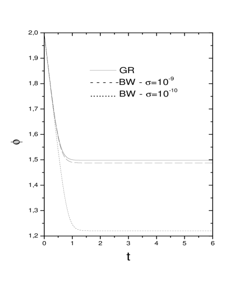
Numerical solutions for the inflaton field $\phi(t)$ are shown in Fig.1 for two different values of the $\sigma$ parameter. Note that the interval from $\phi_{0}$ to $\phi_{\inf}$ increases when the parameter $\sigma$ decreases, but its shapes remain practically unchanged. We should note here that, as long as we decrease the value of the parameter $\sigma$, the quantity $\phi_{0}-\phi_{\inf}$ increases and thus permits $|\Delta\phi_{\inf}|$ to reach $\phi=0$, and the inflaton field does not show oscillations. Inflation begins immediately if the field $\phi$ starts its motion with sufficiently small velocity, in analogy with Einstein’s GR theory. If it starts with large initial velocity $\dot{\phi_{0}}$, and the universe does not present the inflationary period at any stage.

Figure 1: Using the model ($V=const$) the inflaton field $\phi$(t) is plotted as a function of time. Two different values of the $\sigma$ parameter are considered, $\sigma=10^{-9}$ and $\sigma=10^{-10}$. In both cases we have taken the same value of $\dot{\phi_{0}}$. GR is displayed on the same plot, but using Einstein’s theory of Relativity.

.

IV Brane Chaotic Inflation with $V=\lambda_{n}\,\phi^{n}/n$

The most realistic inflationary universe scenarios are chaotic models. In this sense, we consider an effective potential given by $V=\lambda_{n}\,\phi^{n}/n$, for $\phi<\phi_{0}$, which becomes extremely steep for $\phi>\phi_{0}$. When the universe is created at $\phi>\phi_{0}$, where $V_{0}>V(\phi_{0})=\lambda_{n}\phi_{0}^{n}/n$, the field immediately falls down to $\phi_{0}$ and acquires a velocity given by $\dot{\phi}_{0}^{2}/2=V_{0}-V(\phi_{0})$. If the velocity of the field is small, inflation can start immediately. On the other hand, if the velocity is large, the universe never inflates.

In order to proceed, we introduce the parameter $\beta_{0}$, just as in the previous section. During inflation, the scalar factor is given by maartens

$$\frac{a}{a_{o}}=\exp\left(-8\pi\,\int_{\phi_{o}}^{\phi}\,\frac{V[1+V/2\sigma]}{dV/d\phi^{{}^{\prime}}}\,d\phi^{{}^{\prime}}\right),$$ (24)

and the corresponding $N$ e-folds, is given by

$$N=\frac{4\pi\phi_{0}^{2}}{n}\;\left[1+\frac{\lambda_{n}\,\phi_{0}^{n}}{n(n+2)\sigma}\right].$$

Note that the beginning of inflation is determined by the initial value of the inflaton field given by Eq. (18). We resume our main results in table II.

Table 2: Values of $\phi_{inf}$ and $\beta_{0}$ for the models with $n=2$ and $n=4$. Parameter values are given by $\sigma=10^{-10}$ and $V\sim 10^{-11}$

	$\phi_{inf}>$	$\beta_{0}$
$n=2$	$\phi_{0}-4.2$	$6\cdot 10^{-11}$
$n=4$	$\phi_{0}-4.2$	$6\cdot 10^{-11}$

Notice that, for $\phi_{0}=10$, inflation starts at $\phi_{\inf}\sim\,6$, the universe inflates $e^{327}$ times and becomes flat. The universe inflates $e^{60}$ for $\phi_{0}=4.4$ and this leads to $\Omega=1.1$. Note that in analogy with Einstein’s theory of GR and in order to have the value of $\Omega$ in the range 1 $\lesssim\Omega<$ 1.1 we require to a fine tuning of the value of $\phi_{0}$.

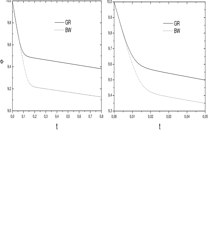
The numerical solution $\phi(t)$ is shown in Fig.2 for two different models, characterized for the values of $n$ and considering the same velocity, $\dot{\phi}_{0}$ in both cases.

Figure 2: This plot shows the solution for the inflaton field $\phi(t)$ as a function of cosmological time $t$, for Einstein’s theory of GR and BW theories. The left panel shows the case $n=2$, and the right one correspond to $n=4$ case. In both cases we have taken $\sigma=10^{-10}$.

.

One of the main prediction of any inflationary universe models is the primordial spectrum that arises due to quantum fluctuation of the inflaton field. Therefore, it is interesting to study the density perturbation behaviors in brane-world cosmology. We estimated density perturbations for our models according to Ref. maartens and thus we may write

$$\frac{\delta\,\rho}{\rho}\,\approx\,Cte\,\left(\frac{V}{V^{\prime}}\right)^{\frac{3}{2}}\left(\,1\,+\,\frac{V}{2\sigma}\right)^{\frac{3}{2}},$$ (25)

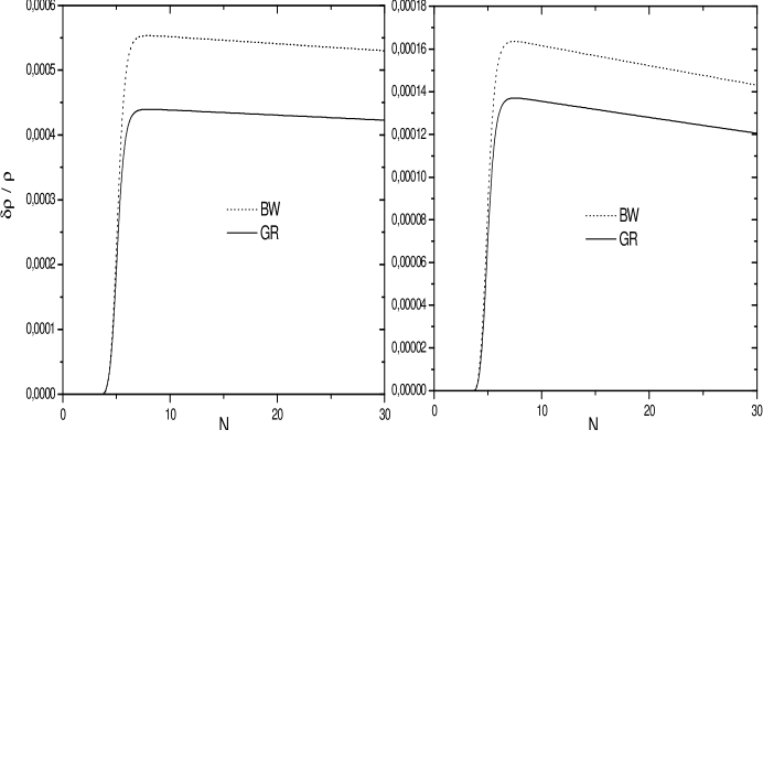
where the latter term corresponds to correction due to BW cosmology for the density perturbations in a flat universe and $Cte=\frac{24}{5}\sqrt{\frac{8\pi}{3}}$. Certainly, these density perturbations should be supplemented by several different contributions for a closed inflationary universe, which alter the result of $\delta\rho/\rho$ at small $N$. We will postpone this important matter for a near future. Fig.(3) shows the magnitude of perturbations in both models, $n=2$ and $n=4$ as a function of $N$ e - folds, for the values $\lambda_{2}=\frac{9}{4}\cdot\,10^{-12}$, $\lambda_{4}=1\cdot\,10^{-14}$ and $\phi_{0}=10$. Note that $\delta\rho/\rho$ has a maximum at small $N\simeq 0(7)$, and presents a small displacement to the right for $\sigma=10^{-10}$. The maximum is located at $N=0(8)$, which corresponds to the scale $\sim$ 10²⁵ cm. This latter result is similar to that obtained in Eisntein’s theory of GR. However, the maximum value of $\delta\rho/\rho$ is bigger in the BW than in for Einstein’s theory of GR.

Figure 3: Scalar density perturbation as a function of the N e-folds. The left panel shows case $n=2$, and the right panel shows the case $n=4$. In both cases we have taken $\sigma=10^{-10}$. These plots are compared with those obtained by using Einstein’s theory of GR, where $\delta\rho/\rho\approx\,CteH^{2}/|\dot{\phi}|.$

.

It is interesting to give an estimation of the tensor spectral index, $n_{T}$, in the Brane-World cosmological model. This index is given in Ref.maartens for a flat universe

$$n_{T}\simeq\,-\frac{1}{8\pi}\left(\frac{V\,^{\prime}}{V}\right)^{2}\,\left[1+\frac{V}{2\sigma}\right]^{-1}.$$ (26)

Solving numerically for $n=2$ and $n=4$ the field equation associated with the scalar field $\phi$, we obtain in Einstein’s theory of GR the following values for the tensor spectral index: $n_{T}\simeq\,-15\cdot\,10^{-4}$ which is evaluated for the value of $N$, where $\delta\rho/\rho$ presents a maximum, i.e, $N\simeq 7$ and for $N\simeq 6$ $n_{T}\simeq\,-65\cdot\,10^{-5}$. In BW cosmological models for $n=2$ we obtain $n_{T}\simeq\,-16\cdot\,10^{-4}$ for $N\simeq 9$ and for $n=4$, $n_{T}\simeq\,-53\cdot\,10^{-5}$ for $N\simeq 8$.

V Comments and Discussion

In this article we study a closed inflationary universes with one self-interacting scalar field in a brane world scenario. For three different models, corresponding respectively to a constant potential and two related to a self-interacting scalar potential given by $V=\lambda_{n}\,\phi^{n}/n$ ($n=2$ and $n=4$). In the former scenarios, we consider a potential with a two regime, one where the potential is constant and another one where the effective potential sharply rises to infinity. In the context of Einstein’s theory of GR, this models was study by Linde Lindeclosed , who showed that this model is not optimistic due to the constancy of the potential implying that the universe collapses very soon or inflates for ever. In our cases, we can fix the graceful exit problem because in BW cosmology we have an extra ingredient that is the model dependencies on the value of the brane tension $\sigma$, that allowed us to reach the value $\phi$=0, which is needed to solve this problem. The problem occurs when $\phi$ reaches the value $\phi=0$, and hence does not show oscillations for the inflaton field necessary for the reheating process. However in the latter scenario, this situation disappears in the chaotic inflationary models, $V(\phi)=\lambda_{n}\,\phi^{n}\,/n$.

We have also found that the inclusion of the additional term ($\rho^{2}$) in the Friedmann’s equation change some of the characteristic of the spectrum of scalar and tensor perturbations. In this sense, the $\delta\rho/\rho$ graphs presents a small displacement to the right with respect to $N$, when compared with that obtained with Einstein‘s theory of GR . This would change the constraint imposed on the value of the parameters that appears in the scalar potentials $\lambda_{n}$. This means that closed inflationary universe models in a Brane-World theory are less restricted than those analogous in Einstein‘s GR theory.

Note that with the fine-tuning at the level of about one percent, one can obtain a semi-realistic model of an inflationary universe with $\Omega>$ 1 as specified by Linde in Ref.Lindeclosed .