Linearized Israel Matching Conditions for Cosmological Perturbations in a Moving Brane Background

Abstract

In the Randall-Sundrum cosmological models, a (3+1)-dimensional brane subject to a $Z_{2}$ orbifold symmetry is embedded in a (4+1)-dimensional bulk spacetime empty except for a negative cosmological constant. The unperturbed braneworld cosmological solutions, subject to homogeneity and isotropy in the three transverse spatial dimensions, are most simply presented by means of a moving brane description. Owing to a generalization of Birkhoff’s theorem, as long as there are no perturbations violating the three-dimensional spatial homogeneity and isotropy, the bulk spacetime remains stationary and trivial. For the spatially flat case, the bulk spacetime is described by one of three bulk solutions: a pure $AdS^{5}$ solution, an $AdS^{5}$-Schwarzschild black hole solution, or an $AdS^{5}$-Schwarzschild naked singularity solution. The brane moves on the boundary of one of these simple bulk spacetimes, its trajectory determined by the evolution of the stress-energy localized on it. We derive here the form of the Israel matching conditions for the linearized cosmological perturbations in this moving brane picture. These Israel matching conditions must be satisfied in any gauge. However, they are not sufficient to determine how to describe in a specific gauge the reflection of the bulk gravitational waves off the brane boundary. In this paper we adopt a fully covariant Lorentz gauge condition in the bulk and find the supplementary gauge conditions that must be imposed on the boundary to ensure that the reflected waves do not violate the Lorentz gauge condition. Compared to the form obtained from Gaussian normal coordinates, the form of the Israel matching conditions obtained here is more complex. However, the propagation of the bulk gravitons is simpler because the coordinates used for the background exploit fully the symmetry of the bulk background solution.

I Introduction

This paper discusses gravitational gauge invariance and gauge fixing for the complete definition of the problem of computing the cosmological perturbations in a one-brane Randall-Sundrum scenario rs , gt1 . In this cosmological scenario, the (4+1)-dimensional bulk spacetime consists of a semi-infinite region, empty except for a negative cosmological constant, bounded by a (3+1)-dimensional timelike surface on which a singular $Z_{2}$-symmetric distribution of stress-energy is localized. The timelike boundary moves in the semi-infinite bulk spacetime, its trajectory determined by the evolution of the stress-energy on it. We assume that the bulk spacetime metric is obtained from a small linearized deviation from an exact solution to the Einstein equations, so that $g_{ab}=g^{(0)}_{ab}+h_{ab}$ in the bulk.

In this paper we establish the form of the boundary conditions coupling the degrees of freedom on the brane to those in the bulk when Lorentz gauge is chosen in the bulk. For the simplest situations such as a Minkowski or de Sitter brane, this is not the simplest gauge choice. For these special situations it is advantageous to employ Gaussian normal coordinates, so that $h_{55}$ and $h_{5\mu}$ vanish. However, for considering realistic cosmological backgrounds, where the universe on the brane has an essentially arbitrary expansion history, Gaussian normal coordinates are particularly awkward, and in many cases develop artificial coordinate singularities. For studying more general, realistic cosmological solutions, it is advantageous to employ instead a “moving brane” description, where the unperturbed bulk remains static and trivial, described by coordinates such as the Poincaré coordinates

$$ds^{2}={1\over z^{2}}\left[dz^{2}-dt^{2}+dx_{1}^{2}+dx_{2}^{2}+dx_{3}^{2}\right]$$ (1)

and the brane “moves,” tracing out a timelike trajectory described as $z=z_{b}(t).$ The moving brane description has been developed in charmousis , in contrast to the fixed brane approach used in binetruy . To consider perturbations in this moving boundary description, it is advantageous to adopt a “covariant” gauge in the bulk, exploiting the full $AdS^{5}$ symmetry of the unperturbed bulk. One such gauge is Lorentz gauge, where

$$\bar{h}_{ab;b}=\nabla_{b}\left[h_{ab}-{1\over 2}g^{(0)}_{ab}\Bigl{(}g^{(0)~{}cd}~{}h_{cd}\Bigr{)}\right]=0.$$ (2)

In this gauge $h_{55}$ and $h_{\mu 5}$ no longer necessarily vanish and the form of the linearized matching condition contains additional terms. Moreover, five additional auxilliary (“gauge”) boundary conditions must be imposed at the brane. One might say that these are the boundary conditions for the five longitudinal (“pure gauge”) modes present in $(4+1)$-dimensional Lorentz gauge. The auxilliary gauge boundary conditions must be chosen in such a way that no forbidden polarization components are emitted or reflected into the bulk from the brane boundary.

In this paper we establish the form of the linearized Israel matching condition and auxilliary gauge conditions for Lorentz gauge. In a forthcoming paper fcp we apply the formal results developed here to the actual problem of computing the evolution of the cosmological perturbations of the coupled brane-bulk system for various expansion histories and various choices for the physical degrees of freedom on the brane.

Linearized braneworld cosmological perturbations have been previously studied by a large number of authors. (See refs. l_start –l_end for a partial sampling of the literature.) The majority of this work relies on the pure scalar-vector-tensor decomposition in the three transverse spatial dimensions, exploiting the three-dimensional homogeneity and isotropy of the background solution, so that the problem problem may be decomposed into separate sectors that are either pure scalar, pure vector, or pure tensor with respect to the three transverse spatial dimensions. As explained in l_start and kodama , generalizing on previous work in gerlach , each such sector contains only a single harmonic with respect to the three transverse spatial dimensions and its dynamics are described by a (1+1)-dimensional partial differential equation in the $yt$-plane. A sector corresponding to a pure tensor harmonic is described by a single coefficient function defined on the $yt$-plane, of scalar character with respect to $y$ and $t,$ whose evolution is described by a $(1+1)$-dimensional partial differential equation. A sector corresponding to a pure vector harmonic has coefficient functions of both scalar and vector character with respect to $y$ and $t;$ however, as Mukohyama l_start and Kodama et al. kodama have shown, these coefficient functions can be expressed in terms of a single “master” scalar function of pure scalar character with respect to $y$ and $t$. Similarly, for the sector corresponding to a pure scalar harmonic, the resulting coefficient functions are of scalar, vector, and tensor character with respect to $y$ and $t.$ However, these in turn may be re-expressed in terms of another single “master variable” of scalar character. The approach adopted in this paper differs in that the gauge is fixed in a way that is completely local and independent of any particular choice of background coordinates or foliation of the background spacetime. It should be noted that the pure scalar-vector-tensor decomposition presupposes a high degree of symmetry and is nonlocal.

The organization of the paper is as follows. In section II we analyse some simplified examples that can be solved by expanding into plane waves in the bulk and individually matching at the boundary. In particular, we consider reflection of electromagnetic waves off a plane perfectly conducting wall under Lorentz gauge, and also the reflection of linearized gravity waves off a planar “gravitational mirror” embedded in a flat (i.e., Minkowski) background. A “gravitational mirror” is a $Z_{2}$-symmetric brane having a vanishing stress-energy at zeroth order. Section III derives the equation of motion of the bulk metric perturbations in a general background in Lorentz gauge and characterizes the residual gauge freedom and its relation to reparameterization invariance on the brane. Section IV considers the generalization of the results of section II to branes curved at zeroth order embedded in bulk backgrounds curved at zeroth order. Section V discusses stress-energy conservation on the brane and derives its expression at linear order. In section VI the general form of the perturbative Israel matching condition and its divergence is presented. This result is then applied to show that the auxilliary boundary conditions proposed in section IV are in fact consistent with Lorentz gauge. Finally, section VII summarizes the results in a concise and self-contained form. Details of the derivation of the evolution equations of the bulk metric perturbations and the consistency of Lorentz gauge in the bulk, of the linearized Israel matching condition, and of the extrinsic curvature perturbations have been, respectively, relegated to three appendices.

Finally, we make explicit the notational conventions used in this paper. We use the metric signature $(-,+,+,+).$ Greek indices $\mu,\nu,\ldots$ denote 4-vectors in (3+1) dimensions; lowercase latin indices denote 5-vectors in a (4+1)-dimensional bulk spacetime (and in some cases, obvious from the context, one of arbitrary dimension as well). The uppercase latin indices $A,B,\ldots$ denote directions parallel to a brane on the boundary of the bulk spacetime, and $N$ denotes the inward unit normal with respect to the boundary. The order of the derivatives with the semicolon convention is as in the example, $W_{A;BC}=A^{a}C^{c}B^{b}\nabla_{c}\nabla_{b}W_{a}.$ The semicolon ; shall denote the covariant derivative with respect to the bulk and $|$ denotes the covariant derivative with respect to the brane. We adopt the convention ${W^{a}}_{;bc}-{W^{a}}_{;cb}={R^{a}}_{dcb}W^{d}$ for the Riemann tensor. On the boundary, we shall frequently use Fermi normal coordinates with respect to the directions on the surface of the brane, continuing these coordinates into the bulk using the Gaussian normal prescription. In this way the connection coefficients vanish at a given point, but in general not their partial derivatives. We shall also define $\nabla_{A}=(A^{a}\nabla_{a})$ for the bulk covariant derivative and define $\tilde{\nabla}_{A}$ to be the corresponding derivation where the tilde indicates that the connection is with respect to the induced metric on the brane. We shall also sometimes suppress raising and lowering of indices, it being implied that this is accomplished using the appropriate zeroth order metric. Accordingly the Einstein convention of summing over repeated indices is implied even when the pairs of repeated indices are both upper or both lower for more orderly looking expressions. We set $\kappa^{2}=(8\pi G)$ where $G$ is Newton’s gravitational constant.

II Some Flat Space Examples: An Accelerating Conductor and Plane Gravitational Mirror in Minkowski Space

In this section we consider some very simple illustrations of what is to follow in which electromagnetic and linearized gravitational waves reflect from a flat planar boundary embedded in flat Minkowski space. In these simple cases the appropriate boundary conditions can be established merely by considering a decomposition into plane waves in the bulk. Later in the paper, when curved boundaries and a curved bulk are considered, the technique of expanding into plane waves can no longer be exploited. Rather it is necessary to modify slightly the boundary conditions obtained in this section to account for the curvature and to employ less direct arguments to demonstrate rigorously their consistency with the bulk gauge condition.

II.1 Reflection of electromagnetic waves off a planar perfectly conducting boundary in Lorentz gauge

We consider classical electrodynamics in Lorentz gauge in a semi-infinite flat spacetime bounded by a planar accelerating perfectly conducting wall. For concreteness we shall assume $(3+1)$ dimensions, even though the generalization to other dimensions is straightforward. Let $z=z_{w}(t)$ be the trajectory of the moving boundary, assumed timelike but otherwise arbitrary. In the semi-infinite region $z>z_{w}(t),$ with $t,$ $x,$ $y$ arbitrary, the wave equation

$$A_{\mu,\nu\nu}=0$$ (3)

describes the forward time evolution. There remains, however, some residual gauge freedom, which may be completely characterized by the scalar solutions to the wave equation

$$\Lambda_{,\nu\nu}=0.$$ (4)

It follows that the gauge transformation

$$A_{\mu}\to A_{\mu}^{\prime}=A_{\mu}-\Lambda_{,\mu}$$ (5)

preserves the Lorentz gauge condition

$$A_{\mu,\mu}=0$$ (6)

and describes the same classical field configuration. The residual gauge freedom is quite limited. Once initial boundary data have been specified (i.e., on a past Cauchy surface), no ambiguity remains as to the evolution of the vector potential forward in time. Once $A_{\mu}$ and its normal derivative have been specified on a Cauchy surface, the future propagation is completely unambiguous, because the initial data for $\Lambda$ may be propagated forward in time from the same Cauchy surface. For a spatially semi-infinite region, however, pure gauge modes may propagate in from the timelike boundary, as indicated in Fig. 1. In order to fix the time evolution completely, some sort of gauge condition on this timelike boundary is required to specify what longitudinal modes, if any, propagate in and how longitudinal modes are reflected off the boundary.

\begin{picture}(7.0,7.0)\centerline{\hbox{\hbox{\psfig{height=199.16928pt}}}} \put(-4.0,-0.5){$S$} \end{picture}

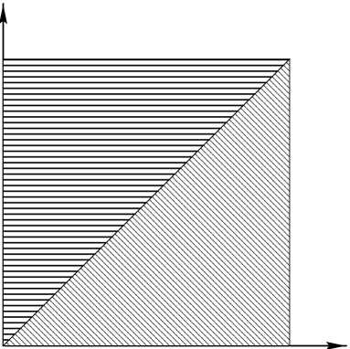
Figure 1: Propagation of the residual gauge ambiguity. Specifying initial data on the Cauchy surface $S,$ taken here to coincide with $t=0,$ $z>0,$ completely specifies the gauge in the diagonally hashed region. However, in the horizontally hashed region, additional gauge information is required to specify how the longitudinal pure gauge modes scatter or propagate in from the timelike boundary at $z=0.$

We first consider a boundary moving at a constant velocity, which may be taken to be situated at $z=0.$ ${\bf E}$ and ${\bf B}$ vanish inside the conducting wall. (We assume that the conductor has no magnetic flux frozen in.) It follows that ${\bf E}_{\parallel}$ and ${\bf B}_{\perp}$ vanish at the boundary, although ${\bf E}_{\perp}$ and ${\bf B}_{\parallel}$ need not vanish there, because these may be generated by surface charge and current density, respectively, on the boundary. We fix the gauge inside the conductor by setting $\underline{\bf A}=(A_{0},{\bf A})=0$ there. It follows that ${\bf A}_{\parallel}$ and $A_{0}$—or, in other words, all the components parallel to the boundary—must vanish. A jump in $A_{\perp},$ however, is not excluded. Such a jump can be generated from a gauge transformation of the ${\bf E}={\bf B}=0$ configuration, for example one where $\Lambda$ vanishes inside the conductor and rises linearly with distance from it on the exterior.

In the bulk $z>0,$ for fixed wavenumber $\underline{\bf k}=({\bf k}_{\parallel},k_{\perp}),$ there are three modes consistent with the Lorentz gauge condition in eqn. (6): two physical modes

$$\hat{\bf e}^{\mu}_{(1)}(\hat{\bf k})~{}\exp[+i\underline{\bf k}\cdot\underline{\bf x}],\quad\hat{\bf e}^{\mu}_{(2)}(\hat{\bf k})~{}\exp[+i\underline{\bf k}\cdot\underline{\bf x}]$$ (7)

and a longitudinal mode

$$\hat{\bf e}^{\mu}_{(L)}(\hat{\bf k})~{}\exp[+i\underline{\bf k}\cdot\underline{\bf x}],$$ (8)

where

$$\hat{\bf e}^{\mu}_{(1)}(\hat{\bf k})={\hat{\bf e}^{\mu}_{x}-\hat{\bf k}^{\mu}(\hat{\bf k}\cdot\hat{\bf e}_{x})\over\sqrt{1-(\hat{\bf k}\cdot\hat{\bf e}_{x})^{2}}},\quad\hat{\bf e}^{\mu}_{(2)}(\hat{\bf k})={\hat{\bf e}^{\mu}_{y}-\hat{\bf k}^{\mu}(\hat{\bf k}\cdot\hat{\bf e}_{y})\over\sqrt{1-(\hat{\bf k}\cdot\hat{\bf e}_{y})^{2}}},\quad\hat{\bf e}^{\mu}_{(L)}(\hat{\bf k})={1\over\sqrt{2}}\Bigl{(}\hat{\bf e}^{\mu}_{t}+\hat{\bf k}^{\mu}\Bigr{)}$$ (9)

and $\hat{\bf k}=\underline{\bf k}/|\underline{\bf k}|,$ $\hat{\bf e}^{\mu}_{t}=(1,0,0,0).$ A fourth polarization

$$\hat{\bf e}_{(F)}={1\over\sqrt{2}}(\hat{\bf e}_{t}-\hat{\bf k}),$$ (10)

which we shall call the forbidden polarization, is excluded by the Lorentz gauge condition.

We have already specified boundary conditions for the components of the 4-vector potential parallel to the conducting boundary, in the present special case $A_{t},$ $A_{x},$ and $A_{y}.$ These components satisfy Dirichlet boundary conditions. It remains to determine the boundary condition for the normal component $A_{\perp},$ $A_{z}$ for the special case here. It is apparent that for incoming longitudinal modes to scatter off the conductor into outgoing longitudinal modes, without creating any of the forbidden fourth polarization, a Neumann boundary condition is required, in other words, $A_{z,z}=0.$ More generally,

$$\hat{\bf t}\cdot\underline{\bf A}=0,\quad\nabla_{\hat{\bf n}}(\hat{\bf n}\cdot\underline{\bf A})=0,$$ (11)

where $\hat{\bf t}$ is an arbitrary vector tangent to the conducting surface and $\hat{\bf n}$ is the normal vector.

This nice separation into physical and pure gauge (longitudinal) modes is not preserved under Lorentz boosts. While a pure gauge mode always transforms into another pure gauge mode, a physical mode transforms into a physical mode with some, in general non-vanishing, admixture of the longitudinal (pure gauge) mode. It is not possible for observers moving relative to each other to agree on a common notion for the absence of a longitudinal component.

For the case of a stationary conducting boundary, it is possible to remove this ambiguity by further fixing the gauge to Coloumb gauge, where $A_{0}=0,$ which is equivalent to postulating the absence of longitudinal photons for the preferred stationary observers. However, when the velocity of the boundary is not constant, physical photons reflected from the boundary will, upon being diffracted back, acquire a longitudinal component from the point of view of an observer at rest with respect to the boundary at a later instant. Consequently, it is necessary to admit longitudinal modes when considering curved or accelerating boundaries.

II.2 Reflection off a planar perfect gravitational mirror

We now consider linearized gravity for a metric perturbation $h_{\mu\nu}$ of Minkoswki space having the background metric $\eta_{\mu\nu}.$ Under a gauge transformation generated by the displacement field $\xi^{\mu}({\bf\underline{x}}),$ the metric perturbation $h_{\mu\nu},$ defined so that $g_{\mu\nu}=\eta_{\mu\nu}+h_{\mu\nu},$ transforms as

$$h_{\mu\nu}\to h_{\mu\nu}^{\prime}=h_{\mu\nu}-\xi_{\mu,\nu}-\xi_{\nu,\mu}.$$ (12)

It is convenient to define the trace-reversed metric perturbation

$$\bar{h}_{\mu\nu}=h_{\mu\nu}-{1\over 2}\eta_{\mu\nu}\eta^{\rho\sigma}h_{\rho\sigma}.$$ (13)

[In our tensor calculus, valid only to first order, indices are raised and lowered with the unperturbed metric $\eta_{\mu\nu}.$] We impose the Lorentz gauge condition

$$\bar{h}_{\mu\nu,\nu}=0.$$ (14)

It follows that a displacement field satisfying

$$\mathord{{\vbox{\hrule height=0.8pt\hbox{\vrule width=0.8pt,height=7.9pt\kern 7.9pt\vrule width=0.8pt} \hrule height=0.8pt}}\hbox{\hskip 1.0pt}}~{}\xi_{\mu}=0$$ (15)

preserves the gauge condition in eqn. (14), and that the equation of motion for the metric perturbation becomes

$$\mathord{{\vbox{\hrule height=0.8pt\hbox{\vrule width=0.8pt,height=7.9pt\kern 7.9pt\vrule width=0.8pt} \hrule height=0.8pt}}\hbox{\hskip 1.0pt}}~{}\bar{h}_{\mu\nu}=-(16\pi G)~{}T_{\mu\nu},$$ (16)

which for a vacuum stress-energy tensor becomes

$$\mathord{{\vbox{\hrule height=0.8pt\hbox{\vrule width=0.8pt,height=7.9pt\kern 7.9pt\vrule width=0.8pt} \hrule height=0.8pt}}\hbox{\hskip 1.0pt}}~{}\bar{h}_{\mu\nu}=0.$$ (17)

If we consider plane waves with the spatial-temporal dependence

$$\exp[i{\bf\underline{k}}\cdot{\bf\underline{x}}]=\exp[i{\bf{k}}\cdot{\bf{x}}-i\omega t],$$ (18)

we find that there are a total of ten possible polarizations for $\bar{h}_{\mu\nu}$: two physical polarizations, four longitudinal (pure gauge) polarizations, and four forbidden polarizations, excluded by the Lorentz gauge condition. Explicitly, these are as follows. The two physical polarizations are

$${\bf\hat{\hat{e}}}_{(+)} = {1\over\sqrt{2}}\Bigl{(}{\bf\hat{e}}_{(1)}\otimes{\bf\hat{e}}_{(1)}-{\bf\hat{e}}_{(2)}\otimes{\bf\hat{e}}_{(2)}\Bigr{)},$$ (19)

$${\bf\hat{\hat{e}}}_{(X)} = {1\over\sqrt{2}}\Bigl{(}{\bf\hat{e}}_{(1)}\otimes{\bf\hat{e}}_{(2)}+{\bf\hat{e}}_{(2)}\otimes{\bf\hat{e}}_{(1)}\Bigr{)}.$$ (20)

The four longitudinal (pure gauge) polarizations are

$${\bf\hat{\hat{e}}}_{(gF)} = {1\over\sqrt{2}}\Bigl{(}{\bf\hat{e}}_{(1)}\otimes{\bf\hat{e}}_{(1)}+{\bf\hat{e}}_{(2)}\otimes{\bf\hat{e}}_{(2)}\Bigr{)},$$ (21)

$${\bf\hat{\hat{e}}}_{(gL)} = {\bf\hat{e}}_{(L)}\otimes{\bf\hat{e}}_{(L)},$$ (22)

$${\bf\hat{\hat{e}}}_{(g1)} = {1\over\sqrt{2}}\Bigl{(}{\bf\hat{e}}_{(1)}\otimes{\bf\hat{e}}_{(L)}+{\bf\hat{e}}_{(L)}\otimes{\bf\hat{e}}_{(1)}\Bigr{)},$$ (23)

$${\bf\hat{\hat{e}}}_{(g2)} = {1\over\sqrt{2}}\Bigl{(}{\bf\hat{e}}_{(2)}\otimes{\bf\hat{e}}_{(L)}+{\bf\hat{e}}_{(L)}\otimes{\bf\hat{e}}_{(2)}\Bigr{)},$$ (24)

and the four forbidden polarizations are

$${\bf\hat{\hat{e}}}_{(fF)} = {\bf\hat{e}}_{(F)}\otimes{\bf\hat{e}}_{(F)},$$ (25)

$${\bf\hat{\hat{e}}}_{(fL)} = {\bf\underline{\underline{\bf g}}},$$ (26)

$${\bf\hat{\hat{e}}}_{(f1)} = {1\over\sqrt{2}}\Bigl{(}{\bf\hat{e}}_{(1)}\otimes{\bf\hat{e}}_{(F)}+{\bf\hat{e}}_{(F)}\otimes{\bf\hat{e}}_{(1)}\Bigr{)},$$ (27)

$${\bf\hat{\hat{e}}}_{(f2)} = {1\over\sqrt{2}}\Bigl{(}{\bf\hat{e}}_{(2)}\otimes{\bf\hat{e}}_{(F)}+{\bf\hat{e}}_{(F)}\otimes{\bf\hat{e}}_{(2)}\Bigr{)}.$$ (28)

Here the double hats denote unit vectors for a second-rank tensor.

As a boundary condition, let us first consider an ideal gravitational mirror in the form of a brane with vanishing stress-energy density localized on the brane and a $Z_{2}$ orbifold symmetry across the brane. We take the geometry of the unperturbed brane to be flat. This idealized invisible brane is the short distance limit of any sort of actual brane, because for any actual nonsingular brane, there is a finite length scale characterizing its vacuum curvature and that inducing by the matter on it.

In the usual Cartesian coordinates, we obtain the following boundary conditions for a normally incident gravitational wave. Let ${\underline{\bf t}}_{1}$ and ${\underline{\bf t}}_{2}$ be arbitrary vectors tangent to the brane. One has the boundary condition

$${\partial\over\partial n}\biggl{(}{\underline{\bf t}}_{1}\cdot\underline{\underline{\bf h}}\cdot{\underline{\bf t}}_{2}\biggr{)}=0,$$ (29)

as derived from the Israel matching conditions, where $\partial/\partial n$ denotes the inward normal derivative. We deduce the boundary conditions for the remaining components by considering the scattering of incoming longitudinal (pure gauge) graviton modes. It is necessary that these scatter exclusively into outgoing longitudinal modes. It is evident that the boundary conditions

$${\underline{\bf n}}\cdot\underline{\underline{\bf h}}\cdot{\underline{\bf t}}_{1} = 0,$$ (30)

$${\partial\over\partial n}\biggl{(}{\underline{\bf n}}\cdot\underline{\underline{\bf h}}\cdot{\underline{\bf n}}\biggr{)} = 0$$ (31)

for the other components satisfy this requirement, for normally as well as for obliquely incident waves.

III Lorentz Gauge in a Curved Background Spacetime

In a curved spacetime, under the gauge transformation generated by an infinitesimal (linearized) displacement field $\xi^{a}$, the linearized metric perturbation transforms according to

$$h_{ab}\to h^{\prime}_{ab}=h_{ab}-{\cal L}_{\xi}g^{(0)}_{ab}=h_{ab}-\xi_{a;b}-\xi_{b;a}.$$ (32)

The trace modified metric perturbation consequently

$${\bar{h}}_{ab}=h_{ab}-{1\over 2}g^{(0)}_{ab}\Bigl{(}g^{(0)~{}cd}~{}h_{cd}\Bigr{)}$$ (33)

transforms as

$${\bar{h}}_{ab}\to{\bar{h}}^{\prime}_{ab}={\bar{h}}_{ab}-\xi_{a;b}-\xi_{b;a}+g^{(0)}_{ab}{\xi^{c}}_{;c}.$$ (34)

For gauge transformations that preserve the Lorentz gauge condition eqn. (2), $\delta\bar{h}_{ab;b}=0,$ which implies that $\xi^{a}$ satisfies

$$\mathord{{\vbox{\hrule height=0.8pt\hbox{\vrule width=0.8pt,height=7.9pt\kern 7.9pt\vrule width=0.8pt} \hrule height=0.8pt}}\hbox{\hskip 1.0pt}}\xi_{a}+{\xi^{b}}_{;ab}-{\xi^{b}}_{;ba}=\mathord{{\vbox{\hrule height=0.8pt\hbox{\vrule width=0.8pt,height=7.9pt\kern 7.9pt\vrule width=0.8pt} \hrule height=0.8pt}}\hbox{\hskip 1.0pt}}\xi_{a}+R_{ab}^{(0)}~{}\xi^{b}=0.$$ (35)

where $\mathord{{\vbox{\hrule height=0.8pt\hbox{\vrule width=0.8pt,height=7.9pt\kern 7.9pt\vrule width=0.8pt} \hrule height=0.8pt}}\hbox{\hskip 1.0pt}}=g^{ab}~{}\nabla_{a}\nabla_{b}.$ The evolution equation for $\bar{h}_{ab}$ is [see Appendix A for a derivation]

$$\mathord{{\vbox{\hrule height=0.8pt\hbox{\vrule width=0.8pt,height=7.9pt\kern 7.9pt\vrule width=0.8pt} \hrule height=0.8pt}}\hbox{\hskip 1.0pt}}\bar{h}_{ab}-\left[g^{(0)}_{bc}\bar{h}_{da}+g^{(0)}_{ac}\bar{h}_{db}+g^{(0)}_{ab}\bar{h}_{cd}-g^{(0)}_{cd}\bar{h}_{ab}\right]R^{(0)}_{cd}+2R^{(0)}_{acbd}~{}\bar{h}_{cd}=-(16\pi G)~{}T^{(1)}_{ab}.$$ (36)

When the background is maximally symmetric, a number of simplifications result. For a (d+1)-dimensional maximally symmetric background spacetime

$$R_{abcd}^{(0)}={R^{(0)}\over{d(d+1)}}\left(g_{ac}^{(0)}~{}g_{bd}^{(0)}-g_{ad}^{(0)}~{}g_{bc}^{(0)}\right),\quad R_{ab}^{(0)}={R^{(0)}\over(d+1)}g_{ab}^{(0)},$$ (37)

so that eqn. (35) becomes

$$\left(\mathord{{\vbox{\hrule height=0.8pt\hbox{\vrule width=0.8pt,height=7.9pt\kern 7.9pt\vrule width=0.8pt} \hrule height=0.8pt}}\hbox{\hskip 1.0pt}}+{R^{(0)}\over{d+1}}\right)\xi^{a}=0,$$ (38)

and eqn. (36) becomes

$$\mathord{{\vbox{\hrule height=0.8pt\hbox{\vrule width=0.8pt,height=7.9pt\kern 7.9pt\vrule width=0.8pt} \hrule height=0.8pt}}\hbox{\hskip 1.0pt}}\bar{h}_{ab}-{R^{(0)}\over{d+1}}\left[-(d-1)\bar{h}_{ab}+g^{(0)}_{ab}\bar{h}_{cc}\right]=-(16\pi G)~{}T^{(1)}_{ab}.$$ (39)

For $AdS^{5}$ presented using the Randall-Sundrum line element

$$ds^{2}=\frac{\ell^{2}}{z^{2}}\left[dz^{2}-dt^{2}+d{\bf x}^{2}\right],$$ (40)

we find that

$$R_{abcd}=-\frac{1}{\ell^{2}}\left(g_{ac}~{}g_{bd}-g_{ad}~{}g_{bc}\right),\quad R_{ab}=-\frac{4}{\ell^{2}}g_{ab},\quad R=-\frac{4\cdot 5}{\ell^{2}},$$ (41)

and $T_{ab}=-\Lambda g_{ab}$ where $\Lambda=-3/(4G\ell^{2}),$ which when substituted in eqn. (39) yields

$$\mathord{{\vbox{\hrule height=0.8pt\hbox{\vrule width=0.8pt,height=7.9pt\kern 7.9pt\vrule width=0.8pt} \hrule height=0.8pt}}\hbox{\hskip 1.0pt}}\bar{h}_{ab}=0.$$ (42)

In (4+1) dimensions the graviton field $h_{ab}$ has $(5\cdot 6)/2=15$ independent components or polarizations. Under the Lorentz gauge condition five of these are rendered forbidden polarizations. The residual gauge freedom may be characterized completely by the solutions to the homogeneous vector wave equation eqn. (35). Here $\xi^{a}({\bf\underline{x}})$ is simply an infinitesimal displacement field generating a coordinate reparameterization. This residual gauge freedom corresponds to five longitudinal (pure gauge) graviton polarizations, leaving a total of five “physical” polarizations. Again, observers moving at a constant velocity with respect to each other cannot agree on a common notation of a purely physical mode without any admixture of longitudinal polarizations.

Before proceeding to a further analysis of the residual gauge freedom in Lorentz gauge, let us first, for comparison, review the counting of allowed polarization states and residual gauge freedom in the Randall-Sundrum gauge (see Ref. rs , gt1 ), where $h_{55}=h_{5\mu}={h^{\mu}}_{\mu}=h_{\mu\nu,\nu}=0.$ There are five remaining polarizations, all of which are physical. Fixing the gauge completely in this way in general displaces the brane from its non-perturbed position at $z=1.$ Consequently, in order to account for all the physical degrees of freedom, it is also necessary to include an additional scalar field, which we shall denote $\xi_{brane\perp}({\bf x}),$ localized on the brane, indicating a normal displacement of the brane with respect to the bulk. [In our notation, the vector ${\bf x}$ denotes a position on the brane whereas ${\bf\underline{x}}$ denotes a position in the bulk.] In Lorentz gauge this last degree of freedom is absent because the corresponding physical degree of freedom is instead described by one of the five longitudinal graviton polarizations. If we dispense with the normal displacement of the brane with respect to the bulk geometry, then the brane is fixed to the surface $z=z_{(b)}(t),$ with $t,$ $x_{1},$ $x_{2}$ and $x_{3}$ arbitrary, no matter what the perturbation is.

Consider now a gauge transformation generated by the displacement field $\xi^{a}({\bf\underline{x}}).$ For this to be pure gauge, we must displace the brane about its unperturbed position $z=z_{(b)}(t)$ according to the normal displacement field $\xi_{brane\perp}({\bf x})=n_{a}\xi^{a}({\bf\underline{x}}).$ However, if instead we fail to compensate for the change in position of the brane by setting $\xi_{brane\perp}({\bf x})$ equal to zero, what would be a pure gauge transformation corresponds to a displacement of the brane trajectory relative to the bulk geometry. The remaining four longitudinal polarizations allowed in Lorentz gauge correspond to reparameterizations of the brane.

The Lorentz gauge condition in the bulk does not in any way fix the gauge on the brane. A gauge transformation corresponding to a reparameterization of the brane is effected by a flux of incoming longitudinal gravitons emanating from the Cauchy surface and reflecting off the brane. More specifically, let the field $\xi_{\parallel}({\bf\underline{x}})$ indicate an infinitesimal reparameterization of the brane. The longitudinal gravitons implementing the desired gauge transformation are generated by choosing $\xi(\underline{{\bf\underline{x}}})$ on the initial Cauchy surface such that $\xi_{\parallel}({\bf\underline{x}})$ on the boundary is reproduced and $\xi_{\perp}({\bf\underline{x}})$ vanishes there. Because we do not include an additional degree of freedom corresponding to normal displacements of the brane, from the view of an observer on the brane, the longitudinal modes in the bulk giving vanishing $\xi_{\parallel}({\bf\underline{x}})$ but non-vanishing $\xi_{\perp}({\bf\underline{x}})$ on the brane are not “pure gauge”. These longitudinal modes take the place of the field localized to the brane $\xi_{brane\perp}({\bf\underline{x}})$ present in the Randall-Sundrum gauge.

IV Compatibility of Sources on the Boundary with the Gauge Condition

In this section we investigate the compatibility of boundary conditions on the timelike boundary (i.e., the brane) with the Lorentz gauge condition. First, as a sort of warm-up exercise, we consider a flat bulk with a planar boundary, which acts as a perfect gravitational mirror. Then we consider the modifications necessary to take into account extrinsic curvature (i.e., nonvanishing stress-energy on the brane at zeroth order) and the spacetime curvature of the bulk at zeroth order for perfect AdS.

IV.1 Special case—the planar perfect gravitational mirror embedded in a Minkowski bulk revisited

We first consider the following boundary conditions for a linearized source on the gravitational mirror boundary (here, in this special case, the bulk is Minkowski space and so is the unperturbed brane)

$$\bar{h}_{AB,N} = -\kappa^{2}_{(5)}{\cal T}_{AB},$$ (43)

$$\bar{h}_{AN} = 0,$$ (44)

$$\bar{h}_{NN,N} = 0.$$ (45)

Here the indices $A,B,\ldots$ indicate directions tangential to the brane, $N$ the normal direction, and $a,b,\ldots$ all five directions. ${\cal T}_{AB}$ denotes here the linearized stress-energy perturbation on the brane. Eqn. (43) is the Israel matching condition and eqns. (44) and (45) are supplementary gauge conditions on the boundary. We show that the Lorentz gauge condition is subsequently satisfied if and only if it is satisfied on the initial Cauchy surface and ${\cal T}_{AB,B}=0$ as well.

To this end, we consider the vector field

$$V_{a}=\bar{h}_{ab,b},$$ (46)

assumed to vanish and have vanishing normal derivative on the initial Cauchy surface. If each component of this 4-vector field can be shown to satisfy either Dirichlet or Neumann homogeneous boundary conditions on the timelike boundary (i.e., the brane), it follows that the Lorentz gauge condition holds everywhere. Physically, this means that wave packets obeying the gauge condition reflect into wave packets obeying the gauge condition and that any inhomogeneous source on the timelike boundary does not emit any waves violating the Lorentz gauge condition.

On the boundary, the relation

$$V_{N}=\bar{h}_{NN,N}+\bar{h}_{AN,A}=0$$ (47)

holds trivially because of the supplementary gauge conditions (44) and (45). Similarly, the normal derivative of the tangential components is given by

$$V_{A,N}=\bar{h}_{AN,NN}+\bar{h}_{AB,BN}=-\bar{h}_{AN,BB}-\kappa^{2}_{(5)}{\cal T}_{AB,B}=-\kappa^{2}_{(5)}{\cal T}_{AB,B}.$$ (48)

Consequently, no Lorentz gauge condition violating waves emanate from the boundary if and only if

$${\cal T}_{AB,B}=0,$$ (49)

in other words, if ${\cal T}_{AB}$ is a conserved tensor field on the brane.

IV.2 The general case—bulks and branes curved at zeroth order

In the previous section we were able to show in a few lines, relying on the wave equation in the bulk and stress-energy conservation on the brane, that (44) and (45) are the correct auxilliary boundary conditions in Lorentz gauge if one assumes that both the brane and the bulk are flat at zeroth order. In this section we essentially repeat the derivation of the previous section for the case where the boundary and the bulk geometry are not flat, including modifications necessary to account for the non-vanishing curvature. When the bulk is curved, the condition $\bar{h}_{AN}=0$ no longer necessarily implies that $\bar{h}_{AN;A}=0$ on the boundary. Consequently, it is necessary to modify eqn. (45) to contain non-derivative contributions of the metric perturbation.

To treat the curved case, we first fix a point ${\bf x}$ on the boundary $\Sigma.$ Then we coordinatize a neighborhood of ${\bf x}$ on $\Sigma$ using the coordinates $x_{A}$ chosen to be Fermi normal coordinates—that is, using exponential map from the tangent space of ${\bf x}$ on $\Sigma$ to $\Sigma.$ By choosing Fermi normal coordinates we set all the Christoffel symbols of the metric connection on $\Sigma$ to zero at ${\bf x},$ although the first and higher partial derivatives of the Christoffel symbols do not in general vanish there. These coordinates may be continued off the boundary by means of the Gaussian normal prescription—that is, the coordinate $n$ in the $N$ direction vanishes on $\Sigma$ and the coordinates on $\Sigma$ are continued along initially normal geodesics, $n$ indicating physical distance along these geodesics from $\Sigma.$ In this way, at ${\bf x}$ we obtain the following connection coefficients for the unit vectors $\hat{e}_{A}=\partial/\partial x_{A}$ and $\hat{e}_{N}=\partial/\partial n:$

$$\nabla_{N}\hat{e}_{N} = 0,$$ (50)

$$\nabla_{A}\hat{e}_{N} = +K_{AB}~{}\hat{e}_{B},$$ (51)

$$\nabla_{N}\hat{e}_{A} = +K_{AB}~{}\hat{e}_{B},$$ (52)

$$\nabla_{A}\hat{e}_{B} = -K_{AB}~{}\hat{e}_{N},$$ (53)

where the tensor $K_{AB}$ is the extrinsic curvature and $\nabla$ denotes the bulk covariant derivative induced by the bulk metric. These equations may be explained as follows. The first equation simply defines the continuation of $N$ off the brane. The second equation consists merely a restatement of the definition of the extrinsic curvature. The third equation follows from the vanishing of the Lie derivative of $N$ along the brane (i.e., $[A,N]=0).$ Finally, the fourth equation follows because $N$ is orthogonal to $\Sigma.$ Away from ${\bf x},$ the last equation would be modified to

$$\nabla_{A}\hat{e}_{B} = \tilde{\Gamma}^{C}_{AB}~{}\hat{e}_{C}-K_{AB}~{}\hat{e}_{N},$$ (54)

where $\tilde{\Gamma}^{C}_{AB}$ denotes the connection coefficients of the covariant derivative on $\Sigma$ with respect to the metric induced on $\Sigma$ by the bulk metric. For future reference, we also give the following second covariant derivatives along the brane

$$\nabla_{D}\nabla_{C}~{}\hat{e}_{N} = +K_{CA;D}~{}\hat{e}_{A}-K_{CA}~{}K_{DA}~{}\hat{e}_{N},$$ (55)

$$\nabla_{D}\nabla_{C}~{}\hat{e}_{B} = \left(\tilde{\Gamma}^{A}_{CB;D}-K_{CB}~{}K_{DA}\right)\hat{e}_{A}-K_{CB;D}~{}\hat{e}_{N}.$$ (56)

IV.2.1 The electromagnetic case

For the electromagnetic case we calculate on the boundary at ${\bf x}$

$$A_{a;a} = A_{A;A}+A_{N;N}$$ (57)

$$= A_{N;N}+\nabla_{A}\left[A_{B}^{(c)}~{}\hat{e}_{B}+A_{N}^{(c)}~{}\hat{e}_{N}\right]\cdot\hat{e}_{A}$$ (58)

$$= A_{N;N}+{\partial A_{B}^{(c)}\over\partial x_{B}}+K_{AA}A_{N}^{(c)}.$$ (59)

Here the superscript $(c)$ denotes that the component in question is to be regarded as a scalar quantity (i.e., differentiated using ordinary partial rather than covariant differentiation). From our boundary condition $A_{B}=0$ (i.e., $\underline{t}\cdot\underline{A}=0$), it follows that the second term vanishes. However, to ensure the reflections and sources from $\Sigma$ do not violate the Lorentz gauge condition, it is necessary to modify the supplementary boundary condition to

$$A_{N;N}+K_{AA}~{}A_{N}=0,$$ (60)

so that eqn. (59) is set to zero.

IV.2.2 Linearized gravitational perturbations

For linearized gravity on a curved boundary only the following boundary condition stays unaltered

$$\bar{h}_{AN}=0.$$ (61)

This is because adding any derivative term would spoil the short distance limit. Consequently, we retain the boundary condition in eqn. (61) and next find the modifications to eqn. (45) required for the curved case. We find that

$$V_{N} = \bar{h}_{NN;N}+\bar{h}_{NA;A}$$ (62)

$$= \bar{h}_{NN;N}$$ (65)

$$+\nabla_{A}\Bigl{[}\bar{h}^{(c)}_{NN}~{}(\hat{e}_{N}\otimes\hat{e}_{N})+\bar{h}^{(c)}_{ND}~{}(\hat{e}_{N}\otimes\hat{e}_{D})$$

$$\quad+\bar{h}^{(c)}_{CN}~{}(\hat{e}_{C}\otimes\hat{e}_{N})+\bar{h}^{(c)}_{CD}~{}(\hat{e}_{C}\otimes\hat{e}_{D})\Bigr{]}\cdot(\hat{e}_{N}\otimes\hat{e}_{A})$$

$$= \bar{h}_{NN;N}+\bar{h}_{NN}~{}K_{AA}-\bar{h}_{BA}~{}K_{AB}.$$ (66)

The above implies that the boundary condition valid for the case with a flat brane and a flat bulk, $\bar{h}_{NN,N}=0$ [eqn. (45)], must be modified to

$$\bar{h}_{NN;N}+K_{AA}~{}\bar{h}_{NN}-K_{AB}~{}\bar{h}_{AB}=0$$ (67)

for the general case. At this point that the boundary condition eqn. (61) remains unaltered is just an inspired guess, vindicated in the calculations that follow.

We now compute the normal derivative of the tangential component of the gauge condition,

$$V_{A;N} = \bar{h}_{AN;NN}+\bar{h}_{AB;BN}$$ (68)

$$= -\bar{h}_{AN;BB}+\bar{h}_{AB;NB}$$ (71)

$$+(\bar{h}_{AN;NN}+\bar{h}_{AN;BB})$$

$$+(\bar{h}_{AB;BN}-\bar{h}_{AB;NB}).$$

The second line of the second expression can be simplified by using the wave equation in eqn. (36) and the Gauss-Codacci relations in eqn. (196)

$$\bar{h}_{AN;NN}+\bar{h}_{AN;BB}=\mathord{{\vbox{\hrule height=0.8pt\hbox{\vrule width=0.8pt,height=7.9pt\kern 7.9pt\vrule width=0.8pt} \hrule height=0.8pt}}\hbox{\hskip 1.0pt}}~{}\bar{h}_{AN}=-2R_{NDAC}~{}\bar{h}_{CD}=-2\left(K_{DA;C}^{(0)}-K_{DC;A}^{(0)}\right)\bar{h}_{CD},$$ (72)

and the third line simplifies using

$$\bar{h}_{AB;BN}-\bar{h}_{AB;NB}=R_{BCNB}~{}\bar{h}_{AC}+R_{ACNB}~{}\bar{h}_{CB}=\left(K_{BA;C}-K_{BC;A}\right)\bar{h}_{CB},$$ (73)

so that

$$V_{A;N} = -\bar{h}_{AN;BB}+\bar{h}_{AB;NB}-\left(K_{BA;C}^{(0)}-K_{BC;A}^{(0)}\right)\bar{h}_{CB}.$$ (74)

We now evaluate $\bar{h}_{AN;BB}$. From the definition of the Laplacian operator

$$\mathord{{\vbox{\hrule height=0.8pt\hbox{\vrule width=0.8pt,height=7.9pt\kern 7.9pt\vrule width=0.8pt} \hrule height=0.8pt}}\hbox{\hskip 1.0pt}} = \left(N^{\mu}N^{\nu}+\sum_{A}A^{\mu}A^{\nu}\right)\nabla_{\mu}\nabla_{\nu}$$ (75)

$$= \left(N^{\mu}\nabla_{\mu}\right)\left(N^{\nu}\nabla_{\nu}\right)-\left(N^{\mu}\nabla_{\mu}N^{\nu}\right)\nabla_{\nu}+\sum_{A}\left[\left(A^{\mu}\nabla_{\mu}\right)\left(A^{\nu}\nabla_{\nu}\right)-\left(A^{\mu}\nabla_{\mu}A^{\nu}\right)\nabla_{\nu}\right]$$ (76)

$$= \nabla_{N}\nabla_{N}+\sum_{A}\left[\nabla_{A}\nabla_{A}+K_{AA}^{(0)}\nabla_{N}\right],$$ (77)

it follows that

$$\bar{h}_{AN;BB}=\left[\nabla_{B}\nabla_{B}+K_{BB}^{(0)}\nabla_{N}\right]\bar{h}_{AN}.$$ (78)

To simplify $\bar{h}_{AN;BB}$ exploiting the fact that $\bar{h}_{AN}=0$ on the brane, we compute

$$\nabla_{D}\nabla_{C}\bar{h}_{AN} = \nabla_{D}\nabla_{C}~{}\Bigl{[}\bar{h}^{(c)}_{NN}~{}(\hat{e}_{N}\otimes\hat{e}_{N})+\bar{h}^{(c)}_{NE}~{}(\hat{e}_{N}\otimes\hat{e}_{E})$$ (80)

$$\quad+\bar{h}^{(c)}_{EN}~{}(\hat{e}_{E}\otimes\hat{e}_{N})+\bar{h}^{(c)}_{EF}~{}(\hat{e}_{E}\otimes\hat{e}_{F})\Bigr{]}\cdot(\hat{e}_{A}\otimes\hat{e}_{N})$$

$$= \nabla_{D}\bar{h}^{(c)}_{NN}~{}(\nabla_{C}\hat{e}_{N})\cdot\hat{e}_{A}+\nabla_{C}\bar{h}^{(c)}_{NN}~{}(\nabla_{D}\hat{e}_{N})\cdot\hat{e}_{A}+\bar{h}^{(c)}_{NN}~{}(\nabla_{D}\nabla_{C}\hat{e}_{N})\cdot\hat{e}_{A}$$ (82)

$$+\bar{h}^{(c)}_{AF}~{}(\nabla_{D}\nabla_{C}\hat{e}_{F})\cdot\hat{e}_{N}+\nabla_{D}\bar{h}^{(c)}_{AF}~{}(\nabla_{C}\hat{e}_{F})\cdot\hat{e}_{N}+\nabla_{C}\bar{h}^{(c)}_{AF}~{}(\nabla_{D}\hat{e}_{F})\cdot\hat{e}_{N}$$

$$= K^{(0)}_{AC}~{}\bar{h}_{NN;D}+K^{(0)}_{AD}~{}\bar{h}_{NN;C}+K^{(0)}_{AC;D}~{}\bar{h}_{NN}$$ (84)

$$-K^{(0)}_{FC;D}~{}\bar{h}_{AF}-K^{(0)}_{CF}~{}\bar{h}_{AF;D}-K^{(0)}_{DF}~{}\bar{h}_{AF;C}.$$

Contracting $C$ and $D,$ we obtain

$$\nabla_{B}\nabla_{B}\bar{h}_{AN} = 2K^{(0)}_{AB}~{}\bar{h}_{NN;B}+K^{(0)}_{AB;B}~{}\bar{h}_{NN}-K^{(0)}_{CB;B}~{}\bar{h}_{AC}-2K^{(0)}_{BC}~{}\bar{h}_{AC;B}.$$ (85)

Consequently,

$$V_{A;N} = \bar{h}_{AB;NB}-\bar{h}_{AN;BB}-\left(K_{BA;C}^{(0)}-K_{BC;A}^{(0)}\right)\bar{h}_{CB}$$ (86)

$$= \bar{h}_{AB;NB}-2K^{(0)}_{AB}~{}\bar{h}_{NN;B}+2K^{(0)}_{BC}~{}\bar{h}_{AB;C}-K^{(0)}~{}\bar{h}_{AN;N}$$ (88)

$$-K^{(0)}_{AB;B}~{}\bar{h}_{NN}+K^{(0)}_{BC;C}~{}\bar{h}_{AB}-\left(K_{BA;C}^{(0)}-K_{BC;A}^{(0)}\right)\bar{h}_{CB}.$$

It remains to be shown using the Israel matching condition and stress-energy conservation on the brane that the above quantity vanishes, so that the corresponding boundary condition on the brane is homogeneous.

V Stress-energy Conservation on the Brane at First Order

In this section we consider how to express stress-energy conservation for a singular distribution of co-dimension one of stress-energy localized on the boundary brane about which a $Z_{2}$ symmetry has been imposed. The simplest way to proceed, which does not require any additional principles for how to treat the singular distribution of boundary matter, is to consider in the limit $\delta\to 0\,+$ a symmetric distribution of non-singular $Z_{2}$ symmetric matter of a finite small thickness $2\delta.$ The bulk spacetime is reflected about the hypersurface at the center of this boundary stress-energy by means of the $Z_{2}$ symmetry, as indicated in Fig. 2. The four-dimensional projected stress-energy tensor on the brane ${\cal T}_{AB}$ is obtained by integrating over the coordinate normal to the brane, denoted by $N,$ whose units correspond to physical distance. One has

$${\cal T}_{AB}({\bf x})=\int_{-\delta}^{+\delta}dN~{}T_{AB}({\bf x},N),$$ (89)

where $T_{AB}$ is the five-dimensional stress-energy tensor. For finite $\delta$ this projection procedure is not entirely satisfactory because of ambiguities in parallel transport. However as $\delta\to 0\,+$ these difficulties disappear.

\begin{picture}(7.0,7.0)\centerline{\hbox{\hbox{\psfig{height=199.16928pt,width=142.26378pt}}}} \put(-3.5,0.0){$\delta$} \put(-2.0,3.0){$N$} \put(-3.5,6.5){$A$} \end{picture}

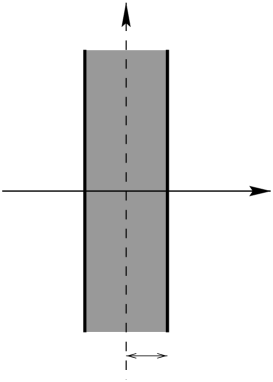
Figure 2: Schematic diagram of the $Z_{2}$ symmetric distribution of brane stress-energy. A singular distribution of stress-energy on the brane is most easily regarded as the limit of a non-singular distribution of stress-energy of support confined to within a shell of thickness $2\delta$ in the limit $\delta\to 0+.$ We derive the boundary conditions applicable for an infinitely thin singular brane by taking the $\delta\to 0+$ limit of a nonsingular thick brane of thickness $\delta.$ The (dashed) line into the middle represents the $Z_{2}$ reflection orbifold symmetry. The projected stress-energy ${\cal T}_{AB}$ (always tangent to the brane) is distributed over the indicated shaded region of thickness $2\delta.$

Using ordinary derivatives, we may write

$$\int_{-\delta}^{+\delta}dN~{}\left(T_{AB,B}+T_{AN,N}\right) = {\cal T}_{AB,B}+T_{AN}(N=+\delta)-T_{AN}(N=-\delta)$$ (90)

$$= {\cal T}_{AB,B}+2T_{AN}(N=+\delta).$$ (91)

Here we may choose, for the purpose of this calculation, Gaussian normal coordinates, so that $N=0$ corresponds to the hypersurface $\Sigma$ of $Z_{2}$ symmetry, and $N$ is the signed normal physical distance from $\Sigma.$ In the neighborhood of a given point ${\bf x}\in\Sigma,$ we may choose the transverse coordinates, labelled $A,B,\ldots,$ so that the connection coefficients vanish at ${\bf x}.$ If $\delta$ is sufficiently small, the difference between $(T_{AB,B}+T_{AN,N})$ and $(T_{AB;B}+T_{AN;N})$ is negligibly small, and it follows that in the $\delta\to 0+$ limit

$${\cal T}_{AB|B}+2T_{AN}(N=+\delta)=0,$$ (92)

where $|$ indicates the covariant derivative on $\Sigma,$ or equivalently (in the $\delta\to 0+$ limit) on the displaced surface $(\Sigma+\delta)$ just outside the singular distribution, on which one imposes the Israel matching condition. Here $-T_{AN}$ represents the five-dimensional flux of energy-momentum incident on the brane from the bulk (the direction $N$ is taken to be outward), or with a plus sign it would represent energy-momentum flowing from the brane into the bulk.

We note that, alternatively, we could have derived eqn. (92) directly from the Israel matching condition and the Gauss-Codazzi relations in eqn. (196).

Because we have assumed an empty bulk (except for the negative cosmological constant), with $T_{ab}=-\Lambda^{(5)}g_{ab}$ outside of the brane, the flux contribution $2T_{AN}$ in eqn. (92) vanishes. This follows because the direction $A$ is normal to $N.$ Extra degrees of freedom (e.g., bulk scalars) in the bulk would in general spoil the vanishing of $T_{AN}.$

In the discussion above, the (projected) brane stress-energy ${\cal T}_{AB}$ has been shown to be a tensor field parallel to the brane in both indices and conserved with respect to the four-dimensional metric induced on the brane. For the components parallel to the brane,

$${\cal T}_{AB|B}={\cal T}_{AB;B}=0,$$ (93)

where $|$ and ; denote covariant derivation with respect to the four-dimensional metric induced on the brane and the full five-dimensional metric, respectively. The discussion so far in the present section applies equally well with and without perturbations.

We now consider perturbations to linear order, splitting ${\cal T}_{AB}={\cal T}^{(0)}_{AB}+{\cal T}^{(1)}_{AB}.$ At zeroth order, stress-energy conservation on the brane is expressed as ${\cal T}^{(0)}_{AB|B}=0,$ where $|$ is the connection with respect to the unperturbed metric induced on the brane.

Stress-energy conservation to linear order is obtained by extracting the first-order terms

$$\left(g_{(0)}^{BC}-h^{BC}\right)\nabla^{[g^{(0)}+h]}_{B}\left({\cal T}_{AC}^{(0)}+{\cal T}_{AC}^{(1)}\right)=0.$$ (94)

Here the superscript $[g^{(0)}+h]$ indicates that the covariant derivation is with respect to the perturbed metric. Keeping only the first order terms of the above equation gives

$${\cal T}^{(1)}_{AB|B}-h^{BC}~{}{\cal T}_{AC|B}^{(0)}+\nabla^{[h]}_{B}~{}{\cal T}_{AB}^{(0)}=0,$$ (95)

where $|$ denotes the connection of the unperturbed metric induced on the brane. Here the operator $\nabla^{[h]}_{A}$ denotes the change in the metric connection due to the perturbation of the metric from $g^{(0)}$ to $(g^{(0)}+h),$ accurate to linear order in $h.$ We may express this operator as

$$\nabla^{[h]}_{A}\hat{e}_{B}={\Gamma^{[h]~{}C}}_{AB}~{}\hat{e}_{C},$$ (96)

where the pseudo-Christoffel symbols above constitute a third-rank tensor (and not a pseudo-tensor) with respect to the unperturbed metric, and can be expressed as

$${\Gamma^{[h]}}_{CAB}={1\over 2}\Bigl{[}h_{AC|B}+h_{BC|A}-h_{AB|C}\Bigr{]}.$$ (97)

At a given point this relation can be demonstrated by choosing Fermi normal coordinates there with respect to the unperturbed metric. Precisely at this point and in these coordinates, $g^{(0)}_{AB,C}=0$ and ${\Gamma^{[g^{(0)}]~{}C}}_{AB}=0.$ It follows from the generally valid expression

$${\Gamma^{C}}_{AB}={1\over 2}g^{CD}\Bigl{[}g_{AD,B}+g_{BD,A}-g_{AB,D}\Bigr{]},$$ (98)

that to linear order

$${\Gamma^{[h]~{}C}}_{AB}={1\over 2}g_{(0)}^{CD}\Bigl{[}h_{AD,B}+h_{BD,A}-h_{AB,D}\Bigr{]}.$$ (99)

Because the unperturbed Christoffel symbols all vanish, these ordinary derivatives may be replaced by covariant derivatives, rendering equation eqn. (99) equivalent to eqn. (97). It follows that

$$\nabla^{[h]}_{B}~{}{\cal T}^{(0)}_{AB} = -{\Gamma^{[h]~{}C}}_{BA}~{}{\cal T}^{(0)}_{CB}-{\Gamma^{[h]~{}C}}_{BB}~{}{\cal T}^{(0)}_{AC}$$ (100)

$$= -{1\over 2}\Bigl{(}h_{BC|A}+h_{CA|B}-h_{BA|C}\Bigr{)}{\cal T}^{(0)}_{CB}$$ (102)

$$-{1\over 2}\Bigl{(}h_{BC|B}+h_{CB|B}-h_{BB|C}\Bigr{)}{\cal T}^{(0)}_{AC}$$

$$= -{1\over 2}\left[2{\cal T}^{(0)}_{AC}~{}h_{BC|B}-{\cal T}^{(0)}_{AC}~{}h_{BB|C}+{\cal T}^{(0)}_{CB}~{}h_{BC|A}\right].$$ (103)

The first-order terms of the stress-energy conservation equation give

$$\left[\nabla_{B}{\cal T}_{AB}\right]^{(1)}={\cal T}^{(1)}_{AB|B}-h_{BC}~{}{\cal T}_{AC|B}^{(0)}+\nabla^{[h]}_{B}~{}{\cal T}_{AB}^{(0)}$$ (104)

$$= {\cal T}^{(1)}_{AB|B}-h_{BC}~{}{\cal T}^{(0)}_{AC|B}-{\cal T}^{(0)}_{AC}~{}h_{BC|B}-{1\over 2}{\cal T}^{(0)}_{BC}~{}h_{BC|A}+{1\over 2}{\cal T}^{(0)}_{AC}~{}h_{BB|C}=0.\quad\quad$$ (105)

VI The Linearized Israel Matching Condition and Its Divergence

In this section we show how to derive the form of the linearized Israel matching condition for a $Z_{2}$ symmetric stress-energy distribution of co-dimension one in a (4+1)-dimensional bulk spacetime. The exact Israel matching condition

$$K_{AB}=-{\kappa^{2}_{(5)}\over 2}\left[{\cal T}_{AB}-{1\over 3}g_{AB}{\cal T}_{CC}\right]$$ (106)

gives $K=+{\kappa^{2}_{(5)}\over 6}{\cal T},$ which may be used to re-write eqn. (106) as

$$K_{AB}-g_{AB}~{}K=-{\kappa_{(5)}^{2}\over 2}~{}{\cal T}_{AB},$$ (107)

giving us at first order the equation

$$K_{AB}^{(1)}-g_{AB}^{(0)}\left(K^{(1)}_{CC}-K^{(0)}_{CD}~{}h_{CD}\right)-h_{AB}~{}K^{(0)}=-{\kappa_{(5)}^{2}\over 2}~{}{\cal T}_{AB}^{(1)}.$$ (108)

The first order perturbation in the extrinsic curvature is [see Appendix C for a derivation]

$$K^{(1)}_{AB}={1\over 2}\left[h_{AB;N}-h_{AN;B}-h_{BN;A}\right]+{1\over 2}K^{(0)}_{AB}~{}h_{NN}.$$ (109)

Using the supplementary boundary condition $h_{AN}=0,$ we may simplify the terms $h_{AN;B}+h_{BN;A}.$ Expanding

$$h_{AN;B} = \nabla_{B}\left[h_{CD}^{(c)}(\hat{e}_{C}\otimes\hat{e}_{D})+h_{NN}^{(c)}(\hat{e}_{N}\otimes\hat{e}_{N})\right]\cdot(\hat{e}_{A}\otimes\hat{e}_{N})$$ (110)

$$= h_{AD}^{(c)}~{}\hat{e}_{N}\cdot(\nabla_{B}\hat{e}_{D})+h_{NN}^{(c)}~{}\hat{e}_{A}\cdot(\nabla_{B}\hat{e}_{N})$$ (111)

$$= -K^{(0)}_{BD}~{}h_{AD}+K_{AB}^{(0)}~{}h_{NN},$$ (112)

we may now re-write

$$K^{(1)}_{AB}={1\over 2}\left[h_{AB;N}+K_{BC}^{(0)}~{}h_{AC}+K_{AC}^{(0)}~{}h_{BC}\right]-{1\over 2}K^{(0)}_{AB}~{}h_{NN},$$ (113)

from which we find that

$$K^{(1)}_{CC}={1\over 2}h_{CC;N}+K_{CD}^{(0)}~{}h_{CD}-{1\over 2}K_{CC}^{(0)}~{}h_{NN}.$$ (114)

The next step is to re-express eqn. (113) in terms of the trace-modified metric perturbation $\bar{h}_{ab}$ rather than $h_{ab}.$ From

$$\bar{h}_{AB}=h_{AB}-{1\over 2}g_{AB}^{(0)}\left(h_{CC}+h_{NN}\right),$$ (115)

it follows that

$$\bar{h}_{AB;N}=h_{AB;N}-{1\over 2}g_{AB}^{(0)}\left(h_{CC;N}+h_{NN;N}\right).$$ (116)

We use the boundary condition [from eqn. (67)]

$$\bar{h}_{NN;N}+K^{(0)}_{AA}~{}\bar{h}_{NN}-K^{(0)}_{AB}~{}\bar{h}_{AB}=0$$ (117)

and

$$\bar{h}_{NN;N}=h_{NN;N}-{1\over 2}g_{NN}^{(0)}\left(h_{CC;N}+h_{NN;N}\right)={1\over 2}\left(h_{NN;N}-h_{CC;N}\right)$$ (118)

to obtain

$$h_{NN;N}=h_{CC;N}+2\bar{h}_{NN;N}=h_{CC;N}-2K_{AA}^{(0)}~{}\bar{h}_{NN}+2K_{AB}^{(0)}~{}\bar{h}_{AB},$$ (119)

which gives

$$\bar{h}_{AB;N}=h_{AB;N}-g_{AB}^{(0)}~{}h_{CC;N}+g_{AB}^{(0)}\left[K_{CC}^{(0)}~{}\bar{h}_{NN}-K_{CD}^{(0)}~{}\bar{h}_{CD}\right].$$ (120)

Using eqns. (112) and (113) and the relations

$$h_{ab}=\bar{h}_{ab}-{1\over 3}g^{(0)}_{ab}\bar{h},\quad h=-{2\over 3}~{}\bar{h},$$ (121)

we expand the left-hand side of the perturbed Israel matching condition in eqn. (108) as

$$K_{AB}^{(1)}-g_{AB}^{(0)}~{}\left(K^{(1)}_{CC}-K^{(0)}_{CD}~{}h_{CD}\right)-K^{(0)}~{}h_{AB}$$ (122)

$$= {1\over 2}\left(h_{AB;N}+K^{(0)}_{AC}~{}h_{BC}+K^{(0)}_{BC}~{}h_{AC}\right)-{1\over 2}K^{(0)}_{AB}~{}h_{NN}$$ (125)

$$-g_{AB}^{(0)}~{}\left({1\over 2}h_{CC;N}+K^{(0)}_{CD}~{}h_{CD}-{1\over 2}K^{(0)}~{}h_{NN}\right)$$

$$+g_{AB}^{(0)}~{}K^{(0)}_{CD}~{}h_{CD}-K^{(0)}~{}h_{AB}$$

$$= {1\over 2}\left(h_{AB;N}-g^{(0)}_{AB}~{}h_{CC;N}\right)+{1\over 2}\left(K^{(0)}_{AC}~{}h_{BC}+K^{(0)}_{BC}~{}h_{AC}\right)$$ (127)

$$-{1\over 2}\left(K^{(0)}_{AB}-g^{(0)}_{AB}~{}K^{(0)}\right)h_{NN}-K^{(0)}~{}h_{AB}$$

$$= {1\over 2}\left[\bar{h}_{AB;N}+g^{(0)}_{AB}~{}\left(K^{(0)}_{CD}~{}\bar{h}_{CD}-K^{(0)}~{}\bar{h}_{NN}\right)\right]$$ (131)

$$+{1\over 2}K^{(0)}_{AC}~{}\left(\bar{h}_{BC}-{1\over 3}g^{(0)}_{BC}~{}\bar{h}\right)+{1\over 2}K^{(0)}_{BC}~{}\left(\bar{h}_{AC}-{1\over 3}g^{(0)}_{AC}~{}\bar{h}\right)$$

$$-{1\over 2}\left[K^{(0)}_{AB}-g^{(0)}_{AB}~{}K^{(0)}\right]\left(\bar{h}_{NN}-{1\over 3}\bar{h}\right)$$

$$-K^{(0)}\left(\bar{h}_{AB}-{1\over 3}g^{(0)}_{AB}~{}\bar{h}\right)$$

$$= {1\over 2}\bar{h}_{AB;N}+{1\over 2}K^{(0)}_{AC}~{}\bar{h}_{BC}+{1\over 2}K^{(0)}_{BC}~{}\bar{h}_{AC}-K^{(0)}~{}\bar{h}_{AB}$$ (134)

$$-{1\over 2}\left[K^{(0)}_{AB}-g^{(0)}_{AB}~{}K^{(0)}\right]\left(\bar{h}_{NN}-{1\over 3}\bar{h}\right)-{1\over 3}K^{(0)}_{AB}~{}\bar{h}$$

$$+g^{(0)}_{AB}\left[{1\over 2}K^{(0)}_{CD}~{}\bar{h}_{CD}-{1\over 2}K^{(0)}~{}\bar{h}_{NN}+{1\over 3}K^{(0)}~{}\bar{h}\right]$$

$$= {1\over 2}\bar{h}_{AB;N}+{1\over 2}K^{(0)}_{AC}~{}\bar{h}_{BC}+{1\over 2}K^{(0)}_{BC}~{}\bar{h}_{AC}-K^{(0)}~{}\bar{h}_{AB}$$ (136)

$$+{1\over 2}g^{(0)}_{AB}~{}K^{(0)}_{CD}~{}\bar{h}_{CD}-{1\over 2}K^{(0)}_{AB}~{}\bar{h}_{NN}-{1\over 6}K^{(0)}_{AB}~{}\bar{h}+{1\over 6}g^{(0)}_{AB}~{}K^{(0)}\bar{h}.$$

We re-write eqn. (108), obtaining for the linearized Israel matching condition

$${1\over 2}\bar{h}_{AB;N}+{1\over 2}K^{(0)}_{AC}~{}\bar{h}_{BC}+{1\over 2}K^{(0)}_{BC}~{}\bar{h}_{AC}-K^{(0)}~{}\bar{h}_{AB}$$ (137)

$$+{1\over 2}g^{(0)}_{AB}~{}K^{(0)}_{CD}~{}\bar{h}_{CD}-{1\over 2}K^{(0)}_{AB}~{}\bar{h}_{NN}-{1\over 6}K^{(0)}_{AB}~{}\bar{h}+{1\over 6}g^{(0)}_{AB}~{}K^{(0)}\bar{h}=-{\kappa_{(5)}^{2}\over 2}~{}{\cal T}_{AB}^{(1)}.\quad\quad$$ (138)

We now proceed to take the divergence of eqn. (138) considered as a tensor field on the brane using the covariant derivation $\tilde{\nabla}$ generated by the induced metric on the brane. Noting that

$$\tilde{\nabla}_{B}\bar{h}_{AB;N} = \bar{h}_{AB;N|B}$$ (139)

$$= \bar{h}_{AB;NB}-K^{(0)}_{AB}~{}\bar{h}_{NB;N}-K^{(0)}_{BB}~{}\bar{h}_{AN;N}+K^{(0)}_{CB}~{}\bar{h}_{AB;C},$$ (140)

we find the divergence of the left-hand side of eqn. (138) is

$$\nabla_{B}\left[K_{AB}^{(1)}-g_{AB}^{(0)}~{}\left(K^{(1)}_{CC}-K^{(0)}_{CD}~{}h_{CD}\right)-K^{(0)}~{}h_{AB}\right]$$ (141)

$$= {1\over 2}\bar{h}_{AB;NB}$$ (147)

$$-{1\over 2}K^{(0)}_{AB}~{}\bar{h}_{NB;N}-{1\over 2}K^{(0)}_{BB}~{}\bar{h}_{AN;N}+{1\over 2}K^{(0)}_{CB}~{}\bar{h}_{AB;C}$$

$$+{1\over 2}K^{(0)}_{BC}~{}\bar{h}_{AC;B}+{1\over 2}K^{(0)}_{AC}~{}\bar{h}_{BC;B}+{1\over 2}K^{(0)}_{BC}~{}\bar{h}_{BC;A}-K^{(0)}~{}\bar{h}_{AB;B}-{1\over 2}K^{(0)}_{AB}~{}\bar{h}_{NN;B}$$

$$-{1\over 6}K^{(0)}_{AB}~{}\bar{h}_{;B}+{1\over 6}K^{(0)}~{}\bar{h}_{;A}$$

$$+{1\over 2}K^{(0)}_{BC;B}~{}\bar{h}_{AC}+{1\over 2}K^{(0)}_{AC;B}~{}\bar{h}_{BC}+{1\over 2}K^{(0)}_{BC;A}~{}\bar{h}_{BC}-K^{(0)}_{;B}~{}\bar{h}_{AB}-{1\over 2}K^{(0)}_{AB;B}~{}\bar{h}_{NN}$$

$$-{1\over 6}K^{(0)}_{AB;B}~{}\bar{h}+{1\over 6}K^{(0)}_{;A}~{}\bar{h}~{}.$$

We next compute the divergence of the right-hand side of eqn. (138), using the result from the stress-energy conservation at first subleading order [eqn. (105)]

$${\cal T}^{(1)}_{AB|B} = {\cal T}_{AC|B}^{(0)}~{}h_{BC}-\nabla^{[h]}_{B}{\cal T}_{AC}^{(0)}$$ (148)

$$= {\cal T}^{(0)}_{AC|B}~{}h_{BC}+{\cal T}^{(0)}_{AC}~{}h_{BC|B}+{1\over 2}{\cal T}^{(0)}_{BC}~{}h_{BC|A}-{1\over 2}{\cal T}^{(0)}_{AC}~{}h_{BB|C}.$$ (149)

Because of the boundary condition $h_{AN}=0,$ $h_{AB|C}=h_{AB;C}.$ The zeroth-order Israel matching condition

$$K_{AB}^{(0)}-g_{AB}^{(0)}~{}K^{(0)}=-{\kappa_{(5)}^{2}\over 2}~{}{\cal T}_{AB}^{(0)}$$ (150)

allows one to express eqn. (149) as

$$-{\kappa_{(5)}^{2}\over 2}{\cal T}^{(1)}_{AB|B} = \left[K_{AC;B}^{(0)}-g_{AC}^{(0)}~{}K^{(0)}_{;B}\right]h_{BC}$$ (152)

$$+K_{AC}^{(0)}~{}h_{BC;B}-K^{(0)}~{}h_{BA;B}+{1\over 2}K_{BC}^{(0)}~{}h_{BC;A}-{1\over 2}K_{AC}^{(0)}~{}h_{BB;C}.$$

Using the definition of the trace-modified metric perturbation [eqn. (121)], we find that

$$-{\kappa_{(5)}^{2}\over 2}{\cal T}^{(1)}_{AB|B} = \left[K_{AC;B}^{(0)}-g_{AC}^{(0)}~{}K_{;B}^{(0)}\right]\left(\bar{h}_{BC}-{1\over 3}g_{BC}^{(0)}~{}\bar{h}\right)$$ (155)

$$+K_{AC}^{(0)}~{}\bar{h}_{BC;B}-K^{(0)}~{}\bar{h}_{BA;B}+{1\over 2}K_{BC}^{(0)}~{}\bar{h}_{BC;A}-{1\over 2}K_{AC}^{(0)}~{}\bar{h}_{BB;C}$$

$$+{1\over 3}K_{AC}^{(0)}~{}\bar{h}_{;C}+{1\over 6}K^{(0)}~{}\bar{h}_{;A},$$

and noting that $\bar{h}=\bar{h}_{BB}+\bar{h}_{NN}$ we can re-write eqn.(155) as

$$-{\kappa_{(5)}^{2}\over 2}{\cal T}^{(1)}_{AB|B} = \left[K_{AC;B}^{(0)}-g_{AC}^{(0)}~{}K_{;B}^{(0)}\right]\left(\bar{h}_{BC}-{1\over 3}g_{BC}^{(0)}~{}\bar{h}\right)$$ (158)

$$+K_{AC}^{(0)}~{}\bar{h}_{BC;B}-K^{(0)}~{}\bar{h}_{BA;B}+{1\over 2}K_{BC}^{(0)}~{}\bar{h}_{BC;A}+{1\over 2}K_{AC}^{(0)}~{}\bar{h}_{NN;C}$$

$$-{1\over 6}K_{AC}^{(0)}~{}\bar{h}_{;C}+{1\over 6}K^{(0)}~{}\bar{h}_{;A}.$$

Subtracting eqn. (158) from eqn. (147) we find that vanishing of the divergence of the Israel matching condition and stress-energy conservation on the brane imply

$$+{1\over 2}\bar{h}_{AB;NB}$$ (159)

$$-{1\over 2}K^{(0)}_{AB}~{}\bar{h}_{NB;N}-{1\over 2}K^{(0)}_{BB}~{}\bar{h}_{AN;N}-{1\over 2}K_{AC}^{(0)}~{}\bar{h}_{BC;B}$$ (160)

$$+K_{BC}^{(0)}~{}\bar{h}_{AC;B}-K_{AB}^{(0)}~{}\bar{h}_{NN;B}$$ (161)

$$+{1\over 2}K_{BC;B}^{(0)}~{}\bar{h}_{AC}-{1\over 2}K_{AC;B}^{(0)}~{}\bar{h}_{BC}+{1\over 2}K_{BC;A}^{(0)}~{}\bar{h}_{BC}-{1\over 2}K_{AB;B}^{(0)}~{}\bar{h}_{NN}$$ (162)

$$+{1\over 6}K_{AB;B}^{(0)}~{}\bar{h}-{1\over 6}K_{;A}^{(0)}~{}\bar{h}=0.$$ (163)

The zeroth order Israel matching condition [eqn. (150)] and stress-energy conservation at zeroth order ${\cal T}^{(0)}_{AB|B}=0$ yield

$$K^{(0)}_{AB;B}-K^{(0)}_{;A}=0,$$ (164)

which may be used to rewrite eqn. (163) as follows

$${1\over 2}\bar{h}_{AB;NB}$$ (165)

$$-{1\over 2}K^{(0)}_{AB}~{}\bar{h}_{NB;N}-{1\over 2}K^{(0)}_{BB}~{}\bar{h}_{AN;N}-{1\over 2}K_{AC}^{(0)}~{}\bar{h}_{BC;B}$$ (166)

$$+K_{BC}^{(0)}~{}\bar{h}_{AC;B}-K_{AB}^{(0)}~{}\bar{h}_{NN;B}$$ (167)

$$+{1\over 2}K_{BC;B}^{(0)}~{}\bar{h}_{AC}-{1\over 2}K_{AC;B}^{(0)}~{}\bar{h}_{BC}+{1\over 2}K_{BC;A}^{(0)}~{}\bar{h}_{BC}-{1\over 2}K_{AB;B}^{(0)}~{}\bar{h}_{NN}=0.$$ (168)

We note that eqn. (168) resulted from assuming the Israel matching condition and stress-energy conservation on the brane. Our object was to show that $V_{A;N},$ given in eqn. (88), vanishes. We note that eqn. (168) equals precisely one half the right-hand side of (88). Hence it follows that $V_{A;N}=0.$

VII Discussion

We summarize our main results as follows. Throughout the paper we have assumed Lorentz gauge in the bulk for the linearized metric perturbations—that is

$$\bar{h}_{ab;b}=0,$$ (169)

where in terms of the linear metric perturbation $h_{ab}$

$$\bar{h}_{ab}=h_{ab}-{1\over 2}g_{ab}^{(0)}~{}\Bigl{(}g^{(0)~{}cd}~{}h_{cd}\Bigr{)}.$$ (170)

In the bulk the Lorentz gauge condition is consistent as long as the bulk stress-energy is conserved. We have demonstrated that the auxiliary boundary conditions on the brane

$$\bar{h}_{AN}=0$$ (171)

and

$$\bar{h}_{NN,N}+K_{AA}~{}\bar{h}_{NN}-K_{AB}~{}\bar{h}_{AB}=0$$ (172)

together with the Israel matching condition sourced by a conserved stress-energy on the brane ${\cal T}_{AB}$ ensure that the waves reflecting from the boundary or emanating from sources there respect the bulk Lorentz gauge condition.

The bulk wave equation in $(4+1)$ dimensions [given in eqn. (36), which simplifies to eqn. (42) for an $AdS^{5}$ bulk] propagates 15 components. On the boundary the Israel matching condition provides 10 of the 15 required boundary conditions. Eqns. (171) and (172) provide the remaining $4+1$ boundary conditions, respectively, required to render reflection off the boundary unique and consistent.

The Lorentz gauge condition in the bulk [eqn. (169)] does not fix the gauge on the brane. Rather, once a choice of gauge on the brane has been chosen, it provides a prescription for continuing this gauge choice into the bulk. In (4+1) dimensions the Lorentz gauge condition allows exactly five longitudinal (pure gauge) modes in the bulk. Four of these correspond to reparameterization of the brane. The one remaining mode corresponds to normal displacements of the brane, which become physical if the brane is fixed to its unperturbed position with respect to the unperturbed background spacetime.

Acknowledgements: MB thanks Mr Denis Avery and the CNRS for support. CC thanks the Gulbenkian Foundation for support and the Laboratoire de Physique Theorique at Orsay for its hospitality. We thank John Stewart for help using REDUCE and Christos Charmousis and especially Pierre Binétruy for useful discussions.

Appendix A Bulk Metric Perturbation Evolution Equations in Lorentz Gauge

In this appendix we derive the evolution equation for the metric perturbation $\bar{h}_{ab}$ and for the violation of the gauge. We assume the Einstein equation $G_{ab}=\left[R_{ab}-{1\over 2}g_{ab}R\right]=(8\pi G)T_{ab}$ and the Lorentz gauge condition $\bar{h}_{ab;b}=0$. We also demonstrate the consistency of the Lorentz gauge condition in the bulk assuming that the bulk stress-energy is conserved. For the linearized perturbations

$$G^{(1)}_{ab}=R^{(1)}_{ab}-{1\over 2}\left[g^{(0)}_{ab}R^{(1)}+h_{ab}R^{(0)}\right]=(8\pi G)T^{(1)}_{ab},$$ (173)

where $R^{(1)}=g^{(0)~{}cd}~{}R^{(1)}_{cd}-h^{cd}~{}R^{(0)}_{cd}.$ The Riemann tensor is given by

$${R^{a}}_{bcd}={\Gamma^{a}}_{bd,c}-{\Gamma^{a}}_{bc,d}+{\Gamma^{a}}_{ec}~{}{\Gamma^{e}}_{bd}-{\Gamma^{a}}_{ed}~{}{\Gamma^{e}}_{bc}$$ (174)

where ${\Gamma^{a}}_{bc}={1\over 2}g^{ad}\left[g_{dc,b}+g_{bd,c}-g_{bc,d}\right]$ can be decomposed as $\Gamma^{a}_{bc}={\Gamma^{[g^{(0)}]}}^{a}_{bc}+{\Gamma^{[h]}}^{a}_{bc},$ where ${\Gamma^{[h]}}^{a}_{bc}={1\over 2}g_{(0)}^{ad}\left[h_{dc;b}+h_{bd;c}-h_{bc;d}\right].$ The linear perturbation of the Riemann tensor is ${R^{(1)}}^{a}_{bcd}={\Gamma^{[h]}}^{a}_{bd;c}-{\Gamma^{[h]}}^{a}_{bc;d},$ and for the Ricci tensor

$$R^{(1)}_{ab}\equiv{R^{(1)}}^{c}_{acb}={1\over 2}\left[-h_{;ab}-h_{ab;cc}+h_{ca;bc}+h_{cb;ac}\right].$$ (175)

From the definition of $\bar{h}_{ab}$ [eqn. (33)], $h_{ab}=\bar{h}_{ab}-(d-2)^{-1}g^{(0)}_{ab}\bar{h},$ $h=-2(d-1)^{-1}\bar{h}.$ Expressing eqn. (173) in terms of $\bar{h}_{ab},$ we find that

$$G^{(1)}_{ab} = {1\over 2}\left[-\bar{h}_{ab;cc}+\bar{h}_{ca;bc}+\bar{h}_{cb;ac}-g^{(0)}_{ab}\bar{h}_{cd;cd}\right]-{1\over 2}\left[-g^{(0)}_{ab}\bar{h}_{cd}+\bar{h}_{ab}g^{(0)}_{cd}\right]R^{(0)}_{cd}$$ (176)

$$= (8\pi G)~{}T^{(1)}_{ab}.$$ (177)

Using $\bar{h}_{ab;cd}-\bar{h}_{ab;dc}=R_{aedc}^{(0)}\bar{h}_{eb}+R_{bedc}^{(0)}\bar{h}_{ae},$ and imposing the Lorentz gauge condition gives

$$\mathord{{\vbox{\hrule height=0.8pt\hbox{\vrule width=0.8pt,height=7.9pt\kern 7.9pt\vrule width=0.8pt} \hrule height=0.8pt}}\hbox{\hskip 1.0pt}}\bar{h}_{ab}-\left[g^{(0)}_{bc}\bar{h}_{da}+g^{(0)}_{ac}\bar{h}_{db}+g^{(0)}_{ab}\bar{h}_{cd}-g^{(0)}_{cd}\bar{h}_{ab}\right]R^{(0)}_{cd}+2R^{(0)}_{acbd}\bar{h}_{cd}=-(16\pi G)~{}T^{(1)}_{ab}.$$ (178)

as the wave equation in Lorentz gauge.

We next demonstrate the consistency of the Lorentz gauge condition with the above evolution equation. To this end, we define the field

$$V_{a}=\bar{h}_{ab;b}$$ (179)

quantifying any possible violation of the Lorentz gauge condition and show that $V_{a}$ satisfies a homogeneous wave equation—that is, one with no non-vanishing sources, as long as the bulk stress-energy is conserved (i.e., $T_{ab;b}=0$). The fact that the wave equation for $V_{a}$ is homogeneous implies that if $V_{a}$ and its normal time derivative on an initial past Cauchy surface vanishes, then $V_{a}$ vanishes everywhere in the future.

We now take the divergence of eqn. (178). The identities

$$D_{ab;mn}-D_{ab;nm} = R_{acnm}{D^{c}}_{b}+R_{bcnm}{D_{a}}^{c},$$ (180)

$$S_{abc;mn}-S_{abc;nm} = R_{adnm}{S^{d}}_{bc}+R_{bdnm}{{S_{a}}^{d}}_{c}+R_{cdnm}{S_{ab}}^{d}$$ (181)

give

$$(\mathord{{\vbox{\hrule height=0.8pt\hbox{\vrule width=0.8pt,height=7.9pt\kern 7.9pt\vrule width=0.8pt} \hrule height=0.8pt}}\hbox{\hskip 1.0pt}}\bar{h}_{ab})_{;b} = \bar{h}_{ab;ccb}=\bar{h}_{ab;cbc}+R_{adbc}\bar{h}_{db;b}+R_{bdbc}\bar{h}_{ad;c}+R_{cdbc}\bar{h}_{ab;d}$$ (182)

$$= \bar{h}_{ab;bcc}+(R_{adbc}\bar{h}_{db}+R_{bdbc}\bar{h}_{ad})_{;c}+R_{adbc}\bar{h}_{db;b}+R_{bdbc}\bar{h}_{ad;c}+R_{cdbc}\bar{h}_{ab;d}$$ (183)

$$= \mathord{{\vbox{\hrule height=0.8pt\hbox{\vrule width=0.8pt,height=7.9pt\kern 7.9pt\vrule width=0.8pt} \hrule height=0.8pt}}\hbox{\hskip 1.0pt}}\bar{h}_{ab;b}-R_{adcb;c}\bar{h}_{db}+R_{dc;c}\bar{h}_{ad}-2R_{adcb}\bar{h}_{db;c}+2R_{dc}\bar{h}_{ad;c}-R_{db}\bar{h}_{ab;d},\quad\quad\quad$$ (184)

which can be used to take the divergence of eqn. (178)

$$(\mathord{{\vbox{\hrule height=0.8pt\hbox{\vrule width=0.8pt,height=7.9pt\kern 7.9pt\vrule width=0.8pt} \hrule height=0.8pt}}\hbox{\hskip 1.0pt}}\bar{h}_{ab})_{;b} - \left[g^{(0)}_{bc}\bar{h}_{da;b}+g^{(0)}_{ab}\bar{h}_{cd;b}\right]R^{(0)}_{cd}+2R^{(0)}_{adbc}\bar{h}_{dc;b}$$ (185)

$$- \left[g^{(0)}_{bc}\bar{h}_{da}+g^{(0)}_{ac}\bar{h}_{db}+g^{(0)}_{ab}\bar{h}_{cd}-g^{(0)}_{cd}\bar{h}_{ab}\right]R^{(0)}_{cd;b}+2R^{(0)}_{adbc;b}\bar{h}_{dc}=-(16\pi G)T^{(1)}_{ab;b}.\quad\quad$$ (186)

Using eqn. (184), we obtain

$$\mathord{{\vbox{\hrule height=0.8pt\hbox{\vrule width=0.8pt,height=7.9pt\kern 7.9pt\vrule width=0.8pt} \hrule height=0.8pt}}\hbox{\hskip 1.0pt}}\bar{h}_{ab;b}-\bar{h}_{cd;a}R^{(0)}_{cd}-\left[g^{(0)}_{ac}\bar{h}_{db}+g^{(0)}_{ab}\bar{h}_{cd}-g^{(0)}_{cd}\bar{h}_{ab}\right]R^{(0)}_{cd;b}+R^{(0)}_{adbc;b}\bar{h}_{dc}=-(16\pi G)T^{(1)}_{ab;b}.\quad\quad\quad$$ (187)

The zeroth order Ricci tensor can be replaced using

$$R^{(0)}_{ab}=(8\pi G)\left[T^{(0)}_{ab}-{1\over{d-1}}g^{(0)}_{ab}T^{(0)}\right].$$ (188)

The Bianchi indentity $R^{(0)}_{ac[bd;b]}=R^{(0)}_{bd[ac;b]}=R^{(0)}_{bdac;b}+R^{(0)}_{bdcb;a}+R^{(0)}_{bdba;c}=0$ gives the relation $R^{(0)}_{bdac;b}-R^{(0)}_{dc;a}+R^{(0)}_{da;c}=0,$ which can be used to re-write

$$R^{(0)}_{acbd;b}\bar{h}_{cd}=R^{(0)}_{bdac;b}h_{cd}=\left(R^{(0)}_{dc;a}-R^{(0)}_{da;c}\right)\bar{h}_{cd}$$ (189)

$$\quad=(8\pi G)\left[{\cal T}^{(0)}_{dc;a}-{\cal T}^{(0)}_{da;c}-{1\over{d-1}}\left(g^{(0)}_{dc}{\cal T}^{(0)}_{;a}-g^{(0)}_{da}{\cal T}^{(0)}_{;c}\right)\right]\bar{h}_{cd},$$ (190)

giving

$$\mathord{{\vbox{\hrule height=0.8pt\hbox{\vrule width=0.8pt,height=7.9pt\kern 7.9pt\vrule width=0.8pt} \hrule height=0.8pt}}\hbox{\hskip 1.0pt}}\bar{h}_{ab;b}=-(16\pi G)~{}\left[{\cal T}^{(1)}_{ab;b}-{1\over 2}{\cal T}^{(0)}_{cd}\bar{h}_{cd;a}+{1\over 2(d-1)}{\cal T}^{(0)}\bar{h}_{;a}-{\cal T}^{(0)}_{ad;b}\bar{h}_{db}\right].$$ (191)

Using the first-order stress-energy conservation equation previously obtained in eqn. (105)

$$\left[\nabla_{b}{\cal T}_{ab}\right]^{(1)} = {\cal T}^{(1)}_{ab;b}-{\cal T}^{(0)}_{ac;b}h_{bc}-{\cal T}^{(0)}_{ac}~{}h_{bc;b}-{1\over 2}{\cal T}^{(0)}_{bc}~{}h_{bc;a}+{1\over 2}{\cal T}^{(0)}_{ac}~{}h_{bb;c}$$ (192)

$$= {\cal T}^{(1)}_{ab;b}-{\cal T}^{(0)}_{ac;b}\bar{h}_{bc}-{1\over 2}{\cal T}^{(0)}_{bc}\bar{h}_{bc;a}+{1\over 2}{1\over{d-1}}{\cal T}^{(0)}\bar{h}_{;a}=0$$ (193)

we obtain $\mathord{{\vbox{\hrule height=0.8pt\hbox{\vrule width=0.8pt,height=7.9pt\kern 7.9pt\vrule width=0.8pt} \hrule height=0.8pt}}\hbox{\hskip 1.0pt}}V_{a}=\mathord{{\vbox{\hrule height=0.8pt\hbox{\vrule width=0.8pt,height=7.9pt\kern 7.9pt\vrule width=0.8pt} \hrule height=0.8pt}}\hbox{\hskip 1.0pt}}\bar{h}_{ab;b}=0,$ proving the consistency of Lorentz gauge at linear order provided that stress-energy is conserved.

Appendix B Derivation of the Perturbed Israel Matching Condition

We derive the Israel matching conditions for a surface of codimension one having singular distribution of stress-energy embedded in a $(d+1)$-dimensional bulk spacetime. The Gauss-Codacci relations capovilla , spivak

$$R_{ABCD} = R^{(ind)}_{ABCD}+K_{AD}K_{BC}-K_{AC}K_{BD},$$ (194)

$$R_{NBCD} = K_{BC;D}-K_{BD;C},$$ (195)

$$R_{NBND} = K_{BC}K_{DC}-K_{BD,N},$$ (196)

decompose the Riemann tensor into a components tangent and normal to the brane. The Ricci tensor and scalar are given by

$$R_{AB} = R_{CACB}+R_{NANB}=R^{(ind)}_{AB}+2K_{AC}K_{CB}-K_{AB}K-K_{AB,N},$$ (197)

$$R_{NA} = K_{BA;B}-K_{;A},$$ (198)

$$R_{NN} = R_{NCNC}=K_{AB}K_{AB}-K_{,N},$$ (199)

and

$$R = R_{AB}g^{AB}+R_{NN}g^{NN}=R^{(ind)}+3K_{AB}K_{BA}-K^{2}-2K_{,N}.$$ (200)

The Einstein equations decompose similarly

$$G_{AB} = G^{(ind)}_{AB}+2K_{AC}K_{CB}-K_{AB}K-K_{AB,N}$$ (202)

$$-{1\over 2}g^{(ind)}_{AB}\left[3K_{CD}K_{DC}-K^{2}-2K_{,N}\right],$$

$$G_{AN} = K_{AB;B}-K_{;A},$$ (203)

$$G_{NN} = {1\over 2}\left[-R^{(ind)}-K_{AB}K_{BA}+K^{2}\right],$$ (204)

where $K=g_{(ind)}^{AB}K_{AB}.$

At the brane itself, where the metric is continuous but its normal derivative may suffer a jump, the singular contribution to $G_{AB}$ arises from the terms

$$-K_{AB,N}+g^{(ind)}_{AB}K_{,N},$$ (205)

which when integrated across the brane give

$$\left[K_{AB}-Kg^{(ind)}_{AB}\right|^{+\delta}_{-\delta}=-\kappa_{(d+1)}^{2}{\cal T}_{AB},$$ (206)

where we define four-dimensional projected stress-energy tensor

$${\cal T}_{AB}=\int^{+\delta}_{-\delta}dN~{}T_{AB},$$ (207)

where $\kappa_{(d+1)}^{2}=8\pi{G}_{(d+1)}=M_{(d+1)}^{-(d-2)}.$ We can trace-modify eqn. (206) to obtain

$$\left[K_{AB}\right|^{+\delta}_{-\delta}=-\kappa_{(d+1)}^{2}\left[{\cal T}_{AB}-{1\over d-1}{\cal T}g^{(ind)}_{AB}\right].$$ (208)

Appendix C Derivation of Extrinsic Curvature Perturbation

To compute the perturbation in the extrinsic curvature derived from a perturbation in the metric we use the relation

$$K_{AB}={+1\over 2}\left[{\cal L}_{\left(\overline{N}+\delta\overline{N}\right)}.\left(\underline{\underline{g}}^{(0)}+\underline{\underline{h}}\right)\right]_{AB}.$$ (209)

This formulation in terms of the Lie derivative circumvents having to consider how covariant differentiation is modified by the metric perturbation. It follows that

$$K^{(1)}_{AB}={1\over 2}\left[{\cal L}_{\overline{N}}~{}\underline{\underline{h}}+{\cal L}_{\delta\overline{N}}~{}\underline{\underline{g}}^{(0)}\right]_{AB}.$$ (210)

For any doubly covariant tensor field $\underline{\underline{\omega}}$ and contravariant vector field $\overline{U},$ the following relation

$$\left({\cal L}_{\overline{U}}~{}\underline{\underline{\omega}}\right)_{ab}=U^{c}~{}\omega_{ab;c}+\omega_{ac}~{}{U^{c}}_{;b}+\omega_{cb}~{}{U^{c}}_{;a}$$ (211)

holds regardless of the choice of covariant derivation ; as long as the connection is torsion free. This property reflects the fact that the Lie derivative is defined solely in terms of the flow induced by $\overline{U}$, and consequently is independent of any metric or affine, torsion free structure defined on the manifold. We find it most convenient to set ; to the metric connection defined by the unperturbed metric $g^{(0)}_{ab},$ in accord with the convention of the rest of this paper. To zeroth order one has $K^{(0)}_{AB}=N_{A;B}.$

We first calculate $\delta\overline{N}$ by requiring that

$$\Bigl{(}N^{a}+\delta N^{a}\Bigr{)}\Bigl{(}g^{(0)}_{ab}+h_{ab}\Bigr{)}\Bigl{(}N^{b}+\delta N^{b}\Bigr{)}=+1,\quad\Bigl{(}N^{a}+\delta N^{a}\Bigr{)}\Bigl{(}g^{(0)}_{ab}+h_{ab}\Bigr{)}X_{A}^{b}=0,$$ (212)

for all directions $X_{A}^{b}$ parallel to the brane. Here $X_{A}^{b}$ is a contravariant unit vector so that $g_{(0)}^{ab}=N^{a}N^{b}+\sum_{A}X_{A}^{a}X_{A}^{b}.$ It follows that $\delta N^{N}={-1\over 2}h_{NN},\delta N^{A}=-{h_{N}}^{A},$ which may be re-written as

$$\delta N^{a}={1\over 2}\Bigl{(}N^{c}h_{cd}N^{d}\Bigr{)}N^{a}-g_{(0)}^{ab}h_{bc}N^{c},$$ (213)

so that

$$\delta N_{a;b} = {1\over 2}h_{NN}N_{a;b}+{1\over 2}N^{c}h_{cd;b}N^{d}N_{a}+N^{c}h_{cd}{N^{d}}_{;b}N_{a}-h_{ac;b}N^{c}-h_{ac}{N^{c}}_{;b}$$ (214)

$$= {1\over 2}h_{NN}K^{(0)}_{ab}+{1\over 2}h_{NN;b}N_{a}+h_{CN}K^{(0)}_{Cb}N_{a}-h_{aN;b}-h_{aC}K^{(0)}_{Cb}.$$ (215)

We now obtain the first order extrinsic curvature perturbation

$$K_{AB}^{(1)} = {+1\over 2}\left[{\cal L}_{\overline{N}}~{}\underline{\underline{h}}+{\cal L}_{\delta\overline{N}}~{}\underline{\underline{g}}^{(0)}\right]_{AB}$$ (216)

$$= {1\over 2}X^{a}_{A}X^{b}_{B}N^{c}h_{ab;c}+{1\over 2}X^{a}_{A}X^{b}_{B}\left[h_{ac}{N^{c}}_{;b}+h_{bc}{N^{c}}_{;a}\right]$$ (218)

$$+{1\over 2}X^{a}_{A}X^{b}_{B}\left[(\delta N)_{a;b}+(\delta N)_{b;a})\right]$$

$$= {1\over 2}h_{AB;N}+{1\over 2}K^{(0)}_{BC}~{}h_{CA}+{1\over 2}K^{(0)}_{AC}~{}h_{CB}$$ (220)

$$+{1\over 2}h_{NN}~{}K^{(0)}_{AB}-{1\over 2}h_{AN;B}-{1\over 2}h_{BN;A}-{1\over 2}K^{(0)}_{BC}~{}h_{CA}-{1\over 2}K^{(0)}_{AC}~{}h_{CB}$$

$$= {1\over 2}h_{AB;N}-{1\over 2}h_{AN;B}-{1\over 2}h_{BN;A}+{1\over 2}h_{NN}~{}K^{(0)}_{AB}.$$ (221)

References

• (1) L. Randall and R. Sundrum, β€œAn Alternative to Compactification,” Phys. Rev. Lett. 83, 4690 (1999); L. Randall and R. Sundrum, β€œA Large Mass Hierarchy From a Small Extra Dimension,” Phys. Rev. Lett. 83, 3370 (1999).
• (2) J. Garriga and T. Tanaka, β€œGravity in the Brane World,” Phys. Rev. Lett. 84, 2778 (2000).
• (3) P. Bowcock, C. Charmousis and R. Gregory, β€œGeneral Brane Cosmologies and their Global Space-Time Structure,” Class. Quant. Grav. 17, 4745 (2000); F. Bonjour, C. Charmousis and R. Gregory, β€œThe Dynamics of Curved Gravitating Walls,” Phys. Rev. D62, 83504 (2000).
• (4) P. BinΓ©truy, C. Deffayet, U. Ellwanger and D. Langlois, β€œBrane Cosmological Evolution in a Bulk With Cosmological Constant,” Phys. Lett. B477, 285 (2000); P. BiΕ„etruy, C. Deffayet and D. Langlois, β€œNonconventional Cosmology From a Brane Universe,” Nucl. Phys. B565, 269 (2000); J. Cline, C. Grojean, G. Servant, β€œCosmological Expansion in the Presence of an Extra Dimension,” Phys. Rev. Lett. 83, 4245 (1999); C. Csaki, M. Graesser, C. Kolda and J. Terning, β€œCosmology of One Extra Dimension With Localized Gravity,” Phys. Lett. B462, 34 (1999).
• (5) W. Israel, β€œSingular Hypersurfaces and Thin Shells in General Relativity,” Nuovo Cim. B44, 1 (1966); Erratum-ibid. B48, 463 (1967).
• (6) U. Gerlach and U. Sengupta, Phys. Rev. D19, 2268 (1978); U. Gerlach and U. Sengupta, Phys. Rev. D20, 3009,(1979); U. Gerlach and U. Sengupta, J. Math. Phys. 20, 2540 (1979).
• (7) S. Mukohyama, β€œGauge invariant gravitational perturbations of maximally symmetric spacetimes,” Phys. Rev. D62, 084015 (2000) (hep-th/0004067).
• (8) H. Kodama, A. Ishibashi and O. Seto, β€œBrane World Cosmology: Gauge Invariant Formalism for Perturbation,” Phys. Rev. D62, 064022 (2000) (hep-ph/0004160).
• (9) D. Langlois, β€œBrane Cosmological Perturbations,” Phys. Rev. D62, 126012 (2000) (hep-th/0005025).
• (10) C. van de Bruck, M. Dorca, R. Brandenberger and A. Lukas, β€œCosmological Perturbations in Brane World Theories: Formalism,” Phys. Rev. D62, 123515 (2000) (hep-th/0005032).
• (11) S. Mukohyama, β€œPerturbation of Junction Condition and Doublky Guage Invariant Variables,” Class. Quanrt. Grav. 17, 4777 (2000) (hep-th/0006146).
• (12) T. Tanaka, β€œAsymptotic Behavior of Perturbations in Randall-Sundrum Brane World,” Prog.Theor.Phys.104, 545 (2000) (hep-ph/0006052).
• (13) S. Mukohyama, β€œPerturbation of Junction Conditions and Doubly Gauge Invariant Variables,” Class. Quant. Grav. 17, 4777 (2000) (hep-th/0006146).
• (14) S. Kobayashi, K. Koyama and J. Soda, β€œQuantum Fluctuations of Bulk Inflation in Inflationary Brane World,” Phys. Lett. B501, 157 (2001) (hep-th/0009160).
• (15) D. Langlois, β€œEvolution of Cosmological Perturbations in a Brane Universe,” Phys. Rev. Lett. 86, 2212 (2001) (hep-th/0010063).
• (16) H. Bridgman, K. Malik and D. Wands, β€œCosmic Vorticity on the Brane,” Phys. Rev. D63, 084012 (2001) (hep-th/0010133).
• (17) D. Langlois, R. Maartens, M. Sasaki and D. Wands, β€œLarge Scale Cosmological Perturbations on the Brane,” Phys. Rev. D63, 084009 (2001) (hep-th/0012044)
• (18) O. Seto and H. Kodama, β€œGravitational Waves in Cosmological Models of Horava-Witten Theory,” Phys. Rev. D63, 123506 (2001) (hep-th/0012102).
• (19) N. Deruelle and J. Katz, β€œGravity on Branes,” Phys. Rev. D64, 083515 (2001) (gr-qc/0104007).
• (20) H. Kudoh and T. Tanaka, β€œSecond-Order Perturbations in the Randall-Sundrum Infinite Brane World,” Phys. Rev. D64, 084022 (2001) (hep-th/0104049)
• (21) S. Mukohyama, β€œIntegro-Differential Equation for Brane World Cosmological Perturbations,” Phys. Rev. D64, 064006 (2001); Erratum, Ibid. D66, 049902 (2002) (hep-th/010418).
• (22) N. Deruelle and T. Dolezel, β€œOn Linearized Gravity in the Randall-Sundrum Scenario,” Phys. Rev. D64, 103506 (2001) (gr-qc/0105118).
• (23) H. Bridgman, K. Malik and D Wands, β€œCosmological Perturbations in the Bulk and on the Brane,” Phys. Rev. D65, 043502 (2002) (astro-ph/0107245).
• (24) K. Koyama and J. Soda, β€œBulk Gravitational Field and Cosmological Perturbations on the Brane,” Phys. Phys. Rev. D65, 023514 (2002).
• (25) D. Gorbunov, V. Rubakov and S. Sibiryakov, β€œGravity Waves From Inflating Brane or Mirrors Moving in $AdS^{5},$” JHEP 0110, 15 (2001) (hep-th/0108017).
• (26) S. Mukohyama, β€œDoubly Covariant Action Principle of Singular Hypersurfaces in General Relativity and Scalar-Tensor Theories,” Phys. Rev. D65, 024028 (2002) (gr-qc/0108048).
• (27) P. Brax, C. van de Bruck and A. Davis, β€œBrane World Cosmology, Bulk Scalars and Perturbations,” JHEP 0110, 026 (2001) (hep-th/0108215).
• (28) B. Leong, P. Dunsby, A. Challinor and A. Lasenby, β€œ(1+3) Covariant Dynamics of Scalar Perturbations in Brane Worlds,” Phys. Rev. D65, 104012 (2002) (gr-qc/0111033).
• (29) S. Mukohyama, β€œBrane Gravity Higher Derivative Terms and Nonlocality,” Phys. Rev. D65, 084036 (2002) (hep-th/0112205).
• (30) K. Koyama, β€œRadion and Large Scale Anisotropy on the Brane,” Phys. Rev. D66, 084003 (2002) (gr-qc/0204047).
• (31) C. Deffayet, β€œOn Brane World Cosmological Perturbations,” Phys. Rev. D66, 103504 (2002) (hep-th/0205084).
• (32) A. Riazuelo, F. Vernizzi, D. Steer and R. Durrer, β€œGauge Invariant Cosmological Perturbation Theory for Brane Worlds,” (hep-th/0205220).
• (33) S. Mukohyama, β€œNonlocality as an Essential Feature of Brane Worlds,” Prog. Theor. Phys. Suppl. 148, 121 (2003) (hep-th/0205231).
• (34) B Leong, A. Challinor, R. Maartens and A. Lasenby, β€œBrane World Tensor Anisotropies in the CMB,” Phys. Rev. D66, 104010 (2002) (astro-ph/0208015).
• (35) A. Ishibashi and T. Tanaka, β€œCan a Brane Fluctuate Freely?” (gr-qc/0208006).
• (36) A. Frolov and L. Kofman, β€œGravitational Waves from Brane World Inflation,” (hep-th/0209133).
• (37) D. Langlois, β€œBrane Cosmology: An Introduction,” Prog. Theor. Phys. Suppl. 148, 181 (2003) (hep-th/0209261).
• (38) N. Deruelle, β€œCosmological Perturbations of an Expanding Brane in an Anti-de Sitter Bulk,” Astrophys. Space Sci. 283, 619 (2003) (gr-qc/0301035).
• (39) K. Koyama and K. Takahashi, β€œPrimordial Fluctuations in Bulk Inflaton Model,” Phys. Rev. D67, 103503 (2003) (hep-th/0301165 ).
• (40) K. Koyama, β€œCosmic Microwave Radiation Anisotropies in Brane Worlds,” Phys. Rev. Lett. 91, 221301 (2003) (astro-ph/0303108).
• (41) K. Koyama and K. Takahashi, β€œExactly Solvable Model for Cosmological Perturbations in Dilatonic Brane Worlds,” Phys. Rev. D68, 103512 (2003) (hep-th/0307073).
• (42) C. Ringeval, T. Boehm and R. Durrer, β€œCMB Anisotropies From Vector Perturbations in the Bulk,” (hep-th/0307100 ).
• (43) R. Battye, C. Van de Bruck and A. Mennim, β€œCosmological Tensor Perturbations in the Randall-Sundrum Model: Evolution in the Near Brane Limit,” Phys. Rev. D69, 064040 (2004) (hep-th/0308134).
• (44) T. Kobayashi and T. Tanaka, β€œBulk Inflaton Shadows of Vacuum Gravity,” Phys. Rev. D69, 064037 (2004) (hep-th/0311197).
• (45) R. Maartens, β€œBrane World Gravity,” Living Rev. Rel. 7, 1 (2004) (gr-qc/0312059).
• (46) H. Yoshiguchi and K. Koyama, β€œBulk Gravitational Field and Drark Radiation in Dilatonic Brane World,” Phys. Rev. D70, 043513, (2004) (hep-th/0403097).
• (47) P. Binetruy, M. Bucher and C. Carvalho, β€œModels for the Brane-Bulk Interaction: Toward Understanding Brane World Cosmological Perturbations,” Phys. Rev. D70, 043509 (2004) (hep-th/0403154).
• (48) P. Brax, C. van de Bruck and A.-C. Davis, β€œBrane World Cosmology,” Rept. Prog. Phys. 67, 2183 (2004) (hep-th/0404011).
• (49) K. Koyama, β€œLate Time Behavior of Cosmological Perturbations in a Single Brane Model,” (astro-ph/0407263).
• (50) T. Kobayashi and T. Tanaka, β€œLeading Order Corrections to the Cosmological Evolution of Tensor Perturbations in Braneworld,” JCAP 0410, 15 (2004) (gr-qc/0408021).
• (51) K. Tomita, β€œJunction Conditions of Cosmological Perturbations,” (astro-ph/0408347).
• (52) K. Koyama, D. Langlois, R. Maartens and D. Wands, β€œScalar Perturbations From Brane World Inflation,” (hep-th/0408222).
• (53) C. Cartier and R. Durrer, β€œTachyonic Perturbations in $AdS^{5}$ Orbifolds,” (hep-th/0409287).
• (54) C. Deffayet, β€œA Note on the Well-Posedness of Scalar Brane World Cosmological Perturbations,” (hep-th/0409302).
• (55) H. Yoshiguchi and K. Koyama, β€œQuantization of Scalar Perturbations in Brane World Inflation,” (hep-th/0411056).
• (56) M. Spivak, A comprehensive introduction to differential geometry, (Berkeley, Calif.: Publish or Perish) (1970-1975).
• (57) R.Β Capovilla and J.Β Guven, β€œGeometry of Deformations of Relativistic Membranes,” Phys. Rev. D51, 6736 (1995) (gr-qc/9411060).
• (58) In preparation.