Abstract

In the previous paper [28] we studied the ’t Hooft-Polyakov (TP) monopole configuration in the $U(2)$ gauge theory on the fuzzy 2-sphere and showed that it has a nonzero topological charge in the formalism based on the Ginsparg-Wilson relation. In this paper, by showing that the TP monopole configuration is stabler than the $U(2)$ gauge theory without any condensation in the Yang-Mills-Chern-Simons matrix model, we will present a mechanism for dynamical generation of a nontrivial index. We further analyze the instability and decay processes of the $U(2)$ gauge theory and the TP monopole configuration.

1 Introduction

Matrix models are promising candidates to formulate the superstring theory nonperturbatively. In IIB matrix model[1], which is the dimensionally reduced model of the 10-dimensional super Yang-Mills theory, both the space-time and the matter are described in terms of matrices, and noncommutative (NC) geometries[2] naturally appear[3, 4].

One of the important subjects of the matrix model is a construction of configurations with nontrivial indices in finite NC geometries. It is not only interesting from the mathematical point of view but necessary from the physical requirement. Namely, compactifications of extra dimensions with nontrivial indices can realize chiral gauge theories in our space-time. Nontrivial configurations in NC geometries have been constructed by using algebraic K-theory and projective modules [5, 6, 7, 8, 9, 10]. However the relation to indices of Dirac operators are not clear in these formulations.

The formulation of NC geometries in Connes’ prescription is based on the spectral triple (${\cal A}$,${\cal H}$,${\cal D}$), where a chirality operator and a Dirac operator which anti-commute are introduced[2]. Since NC geometries on compact manifolds have only finite degrees of freedom, a more suitable framework to discuss the problems mentioned above will be to modify the Connes’ spectral triple so that the chirality operator and the Dirac operator satisfy the Ginsparg-Wilson (GW) relation[11]. GW relation has been developed in the lattice gauge theory. The exact chiral symmetry[12, 13] and the index theorem[14, 12] at a finite cutoff can be realized by using the GW Dirac operator[15].

In ref.[16], we have provided a general prescription to construct chirality operators and Dirac operators satisfying the GW relation in general gauge field backgrounds on finite NC geometries. As a concrete example we considered the fuzzy 2-sphere[17]. On the fuzzy 2-sphere two types of Dirac operators, $D_{\rm WW}$[18] and $D_{\rm GKP}$[19, 20], had been constructed. $D_{\rm WW}$ has doublers and the correct chiral anomaly cannot be reproduced. On the other hand, $D_{\rm GKP}$ breaks chiral symmetry at finite matrix size, and the chiral structures are not clear, though the chiral anomaly can be reproduced correctly in the commutative limit[21, 6, 22, 23]. Hence the formalism based on the GW relations is more suitable to study chiral structures on the fuzzy 2-sphere. The GW Dirac operator in vanishing gauge field was constructed in [24, 25]. In ref.[16], we constructed GW Dirac operator in general gauge field configurations. Owing to the GW relation, an index theorem can be proved even for finite NC geometries. We have defined a topological charge, and showed that it takes only integer values, and becomes the Chern character in the commutative limit [16, 26, 27, 28].

We then studied the ’t Hooft-Polyakov (TP) monopole configuration as a topologically nontrivial configuration in [28]. We showed that this configuration is a NC analogue of the commutative TP monopole by explicitly studying the form of the configuration. We then redefined the topological charge by inserting a projection operator, and showed that it reproduces the correct form of the topological charge in the commutative limit, namely, the magnetic flux for the unbroken $U(1)$ component. We also showed that the value of the topological charge is one for the TP monopole configuration. Therefore, if the $U(2)$ gauge theory on the fuzzy 2-sphere decays to the TP monopole configuration, it means a nontrivial index is generated dynamically. It can also be interpreted as a spontaneous symmetry breaking: $U(2)\rightarrow U(1)\times U(1)$ on the fuzzy 2-sphere.

In this paper, by showing that the TP monopole configuration is stabler than the $U(2)$ gauge theory without condensation in the Yang-Mills-Chern-Simons matrix model [33][20], we will present a mechanism of the dynamical generation of an index through the spontaneous symmetry breaking. In this matrix model, the $U(2)$ gauge theory on the fuzzy 2-sphere corresponds to the 2-coincident fuzzy 2-spheres. The TP monopole configuration is equivalent to the 2-concentric fuzzy 2-spheres whose matrix sizes are different by two. More general 2-concentric fuzzy 2-spheres whose matrix sizes are different by integers $2m$ correspond to a monopole configuration with the topological charge $-|m|$. We will also discuss these general monopole configurations.

The stability of these configurations are investigated in papers [33, 20, 34, 35, 36, 37, 38, 39, 40]. Especially $k$-coincident fuzzy spheres are analyzed in [37]. The configuration gives the $U(k)$ gauge theory on the fuzzy sphere. In [37] the dynamics was studied both analytically and numerically, and the $U(k)$ gauge theory has been shown to be unstable. It decays, and finally arrives at the single fuzzy sphere configuration, the $U(1)$ gauge theory on the fuzzy sphere.

In this paper, by studying free energies for the 2-concentric fuzzy spheres whose matrix sizes are different by arbitrary integers $2m$, we investigate how 2-coincident fuzzy spheres decay to the single fuzzy sphere. The configuration with the matrix-size-difference $2(m+1)$ is stabler than the one with $2m$ at the classical level, and quantum corrections do not change this property. Thus a configuration of the 2-coincident spheres ($m=0$) decays into the TP monopole configuration of $m=1$. By repeating such transitions, it cascades into the single fuzzy sphere configuration.

We further study the decay modes around the configuration of the 2-coincident spheres ($m=0$) and the TP monopole configuration ($m=1$) by calculating effective actions along the directions of the collective (zero) modes. The case for $m=0$ receives subtle quantum corrections: The zero-mode directions become unstable for small values of the total matrix size $N$, and metastable for large N, but the metastability becomes negligible at large $N$ limit. The case for $m=1$ is metastable at the classical level, and quantum corrections do not change this property.

In section 2 we briefly review how to define the Dirac operator and the chirality operator on the fuzzy 2-sphere, where the GW relation and thus the index theorem are satisfied naturally. Then we review the monopole configurations with the nontrivial topological charges. In section 3, we introduce the Yang-Mills-Chern-Simons matrix model[33][20], and then investigate the instability of the monopole configurations in this model. We show that for $U(2)$ gauge theory the monopole configurations of larger $m$ are stabler, which means the symmetry is spontaneously broken and the index is generated dynamically. Section 4 is devoted to conclusions and discussions. In appendix A the one-loop effective action is calculated for the matrix model.

2 Configurations with nontrivial topological charges

In this section, after briefly reviewing the ordinary Dirac operator on the fuzzy sphere in subsection 2.1, we see how to construct the Dirac operator and chirality operator satisfying the GW relation in subsection 2.2. We also explain the construction of the topological charge and the index theorem on the fuzzy 2-sphere. Then we explain the monopole configurations with nontrivial topological charges in subsection 2.3.

2.1 Dirac operator on fuzzy 2-sphere

NC coordinates of the fuzzy 2-sphere are described by

$$x_{i}=\alpha L_{i},$$ (2.1)

where $\alpha$ is the NC parameter, and $L_{i}$’s are $n$-dimensional irreducible representation matrices of $SU(2)$ algebra:

$$[L_{i},L_{j}] = i\epsilon_{ijk}L_{k}.$$ (2.2)

Then we have the following relation,

$$(x_{i})^{2} = \alpha^{2}\frac{n^{2}-1}{4}{\mathbb{1}}_{n}\equiv\rho^{2}{\mathbb{1}}_{n},$$ (2.3)

where $\rho$ expresses the radius of the fuzzy 2-sphere. The commutative limit can be taken by $\alpha\to 0,n\to\infty$ with $\rho$ fixed.

Any wave functions on fuzzy 2-sphere are written as $n\times n$ matrices. We can expand them in terms of NC analogues of the spherical harmonics $\hat{Y}_{lm}$, which are traceless symmetric products of the NC coordinates, and has an upper bound for the angular momentum $l$ as $l\leq n-1$. Derivatives along the Killing vectors on the sphere are written as the adjoint operator of $L_{i}$ on any hermitian matrix $M$:

$${\tilde{L}}_{i}M=[L_{i},M]=(L_{i}^{L}-L_{i}^{R})M$$ (2.4)

$$\leftrightarrow {{\cal L}_{i}}M=-i\epsilon_{ijk}x_{j}\partial_{k}M.$$ (2.5)

In eq.(2.4) the superscript L (R) in $L_{i}$ means that this operator acts from the left (right) on matrices. Eq.(2.5) expresses the commutative limit of eq.(2.4). An integral over the 2-sphere is given by a trace over matrices:

$$\frac{1}{n}\hbox{tr}\leftrightarrow\int\frac{d\Omega}{4\pi}.$$ (2.6)

There are two types of Dirac operators constructed on the fuzzy 2-sphere [18][19, 20]. Here we consider the following Dirac operator $D_{\rm GKP}$. The fermionic action is defined as

$$S_{\rm GKP} = \hbox{tr}[\bar{\Psi}D_{\rm GKP}\Psi],$$ (2.7)

$$D_{\rm GKP} = \sigma_{i}({\tilde{L}}_{i}+\rho a_{i})+1,$$ (2.8)

where $a_{i}$ is a gauge field. This action is invariant under the gauge transformation:

$$\Psi \rightarrow U\Psi,$$

$$\bar{\Psi} \rightarrow \bar{\Psi}U^{\dagger},$$

$$a_{i} \rightarrow Ua_{i}U^{\dagger}+\frac{1}{\rho}(UL_{i}U^{\dagger}-L_{i}),$$ (2.9)

since a combination

$$A_{i}\equiv L_{i}+\rho a_{i}$$ (2.10)

transforms covariantly as

$$A_{i}\rightarrow UA_{i}U^{\dagger}.$$ (2.11)

The normal component of $a_{i}$ to the sphere can be interpreted as the scalar field on the sphere. We define it covariantly as

$$\phi=\frac{1}{n\rho}\left(A_{i}^{2}-\frac{n^{2}-1}{4}\right).$$ (2.12)

In the commutative limit this scalar field (2.12) becomes $a_{i}n_{i}$, where $n_{i}=x_{i}/\rho$. If we take the commutative limit of (2.8), the Dirac operator $D_{\rm GKP}$ becomes

$$D_{\rm GKP}\rightarrow D_{\rm com}=\sigma_{i}({\cal L}_{i}+\rho a_{i})+1,$$ (2.13)

which is the ordinary Dirac operator on the commutative 2-sphere.

Due to the noncommutativity of the coordinates, $D_{\rm GKP}$ does not anti-commute with the chirality operator. Then, by carefully evaluating this nonzero anticommutation relation, the chiral anomaly can be reproduced correctly [21, 6, 22, 23]. However, chiral structures are not transparent in this formulation, and we will define another Dirac operator suitable for these issues.

2.2 GW Dirac operator and index theorem

In order to discuss chiral structures on the fuzzy 2-sphere, we define a Dirac operator satisfying the GW relation. Such a Dirac operator was constructed for the free case in [24, 25], and for general gauge field configurations in [16]. According to the formulatoin in [16], we first define two chirality operators:

$$\Gamma^{R} = a\left(\sigma_{i}L_{i}^{R}-\frac{1}{2}\right),$$ (2.14)

$$\hat{\Gamma} = \frac{H}{\sqrt{H^{2}}},$$ (2.15)

where

$$H=a\left(\sigma_{i}A_{i}+\frac{1}{2}\right),$$ (2.16)

and

$$a=\frac{2}{n}$$ (2.17)

is introduced as a NC analogue of a lattice-spacing. These chirality operators satisfy

$$(\Gamma^{R})^{\dagger}=\Gamma^{R},\ (\hat{\Gamma})^{\dagger}=\hat{\Gamma},\ (\Gamma^{R})^{2}=(\hat{\Gamma})^{2}=1.$$ (2.18)

We next define the GW Dirac operator as

$$D_{\rm GW}=-a^{-1}\Gamma^{R}(1-\Gamma^{R}\hat{\Gamma}).$$ (2.19)

Then the action

$$S_{\rm GW}=\hbox{tr}[\bar{\Psi}D_{\rm GW}\Psi]$$ (2.20)

is invariant under the gauge transformation (2.9). If we take the commutative limit, $D_{\rm GW}$ becomes

$$D_{\rm GW}\rightarrow D^{\prime}_{\rm com}=\sigma_{i}({\cal L}_{i}+\rho P_{ij}a_{j})+1,$$ (2.21)

where $P_{ij}=\delta_{ij}-n_{i}n_{j}$ is the projector to the tangential directions on the sphere.

By the definition (2.19), the GW relation

$$\Gamma^{R}D_{\rm GW}+D_{\rm GW}\hat{\Gamma}=0$$ (2.22)

is satisfied. Then we can prove the following index theorem:

$${\rm{index}}D_{\rm GW}\equiv(n_{+}-n_{-})=\frac{1}{2}{\cal T}r(\Gamma^{R}+\hat{\Gamma}),$$ (2.23)

where $n_{\pm}$ are the numbers of zero eigenstates of $D_{\rm GW}$ with a positive (or negative) chirality (for either $\Gamma^{R}$ or $\hat{\Gamma}$) and ${\cal T}r$ is a trace of operators acting on matrices.

The rhs of (2.23) have the following properties. Firstly, it takes only integer values since both $\Gamma^{R}$ and $\hat{\Gamma}$ have a form of sign operator by the definitions (2.14), (2.15). Secondly it becomes the Chern character on the 2-sphere in the commutative limit. Finally, in order to discuss a topological charge for topologically nontrivial configurations in a spontaneously symmetry broken gauge theory, we need to slightly modify it, as will be seen in the next subsection.

2.3 Monopole configurations

As a configuration with a nontrivial topological charge, the TP monopole configuration was constructed in the $U(2)$ gauge theory on the fuzzy 2-sphere [27, 28]. The TP monopole configuration is given by

$$A_{i}=L_{i}^{(n)}\otimes{\mathbb{1}}_{2}+{\mathbb{1}}_{n}\otimes\frac{\tau_{i}}{2}.$$ (2.24)

where $A_{i}$’s are the combination (2.10). $L_{i}^{(n)}$ is the $n$ dimensional representation of $SU(2)$ algebra. The first and the second factors represent the coordinates of the NC space and a configuration of the $U(2)$ gauge field respectively. The total matrix size is $N=2n$. The gauge field is given by

$$a_{i}=\frac{1}{\rho}{\mathbb{1}}_{n}\otimes\frac{\tau_{i}}{2}.$$ (2.25)

By taking the commutative limit of (2.25), and decomposing it into the normal and the tangential components of the sphere, it can be shown to correspond to the TP monopole configuration. See [28] for details.

Note that $A_{i}$’s in (2.24) satisfy the $SU(2)$ algebra:

$$[A_{i},A_{j}]=i\epsilon_{ijk}A_{k},$$ (2.26)

and can be decomposed into irreducible representations:

$$A_{i}=U\begin{pmatrix}L_{i}^{(n+1)}&\cr&L_{i}^{(n-1)}\cr\end{pmatrix}U^{\dagger}.$$ (2.27)

Hence the TP monopole configuration can be geometrically regarded as the $2$-concentric fuzzy spheres whose matrix sizes differ by two.

More generally, we consider $2$-concentric fuzzy spheres whose matrix sizes differ by arbitrary integers $2m$:

$$A_{i}=\begin{pmatrix}L_{i}^{(n+m)}&\cr&L_{i}^{(n-m)}\cr\end{pmatrix}.$$ (2.28)

The $m=0$ case corresponds to the 2-coincident fuzzy 2-spheres, whose effective action is the $U(2)$ gauge theory on the fuzzy 2-sphere. The $|m|=1$ case corresponds to the TP monopole configuration. The $|m|=n$ case corresponds to the single fuzzy 2-sphere, whose effective action is the $U(1)$ gauge theory on the fuzzy 2-sphere. As we will see in (2.35), the configuration of $m$ ($|m|\ll n$) corresponds to the monopole configurations with magnetic charge $-|m|$.

For the configurations of $m\neq 0$, $U(2)$ gauge symmetry is broken to $U(1)\times U(1)$. Thus it is natural to modify the topological charge of the rhs in (2.23) so that it contains only the unbroken gauge fields. We then define the following modified topological charge:

$$\frac{1}{2}{\cal T}r[\phi^{\prime}(\Gamma^{R}+\hat{\Gamma})],$$ (2.29)

where $\phi^{\prime}$ is given by

$$\phi^{\prime}=\frac{1}{n|m|}\left(A_{i}^{2}-\frac{n^{2}+m^{2}-1}{4}\right)=\frac{m}{2|m|}\begin{pmatrix}{\mathbb{1}}_{n+m}&\cr&-{\mathbb{1}}_{n-m}\cr\end{pmatrix}.$$ (2.30)

$\phi^{\prime}\simeq\frac{\rho}{|m|}\phi$ when $|m|\ll n$. $\phi^{\prime}$ is a normalized scalar field in such a sense that it satisfies $\sum_{a}(\phi^{\prime a})^{2}=1$, if we rewrite $a_{i}=a_{i}^{a}\tau^{a}/2$ and $\phi^{\prime}=\phi^{\prime a}\tau^{a}/2$ in the commutative limit. The modified topological charge (2.29) becomes

$$\frac{\rho^{2}}{8\pi}\int_{S^{2}}d\Omega\epsilon_{ijk}n_{i}\phi^{\prime a}F_{jk}^{a},$$ (2.31)

where $F_{jk}=F_{jk}^{a}\tau^{a}/2$ is the field strength defined as $F_{jk}=\partial_{j}a_{k}^{\prime}-\partial_{k}a_{j}^{\prime}-i[a_{j}^{\prime},a_{k}^{\prime}]$, and $a^{\prime}_{i}={\epsilon_{ijk}x_{j}a_{k}/\rho}$. This is nothing but the Chern character with the projection to pick up the component $\phi^{\prime a}$, namely, magnetic charge for the unbroken $U(1)$ component in the TP monopole configuration.

Since $A_{i}$’s satisfy $SU(2)$ algebra (2.26), we can show by straightforward calculations [28]

$$\frac{1}{2}{\cal T}r[P^{(n\pm m)}(\Gamma^{R}+\hat{\Gamma})]=\mp m,$$ (2.32)

for the configuration (2.28). Here $P^{(n\pm m)}$ is the projection operator to pick up the Hilbert space for the $n\pm m$ dimensional irreducible representation, respectively. These projection operators can be written as

$$P^{(n\pm m)} = \frac{(A_{i})^{2}-\frac{1}{4}[(n\mp m)^{2}-1]}{\frac{1}{4}[(n\pm m)^{2}-1]-\frac{1}{4}[(n\mp m)^{2}-1]}$$ (2.33)

$$= \pm\frac{|m|}{m}\phi^{\prime}+\frac{1}{2}.$$ (2.34)

Hence we can see

$$\frac{1}{2}{\cal T}r[\phi^{\prime}(\Gamma^{R}+\hat{\Gamma})]=-|m|.$$ (2.35)

Therefore, the configuration (2.28) represent a monopole configuration with a magnetic charge $-|m|$. In particular, the configuration (2.27) of $m=1$ is the familiar TP monopole with a magnetic charge $-1$. This was also seen by looking at the explicit form of the configuration in (2.25).

Therefore, if by some mechanism, the $U(2)$ gauge theory, the 2-coincident fuzzy spheres of $m=0$ decays to the TP monopole configuration of $|m|=1$, or to the more general monopole configurations of $|m|\geq 1$, it means the index is generated dynamically. Also it is understood as a spontaneous symmetry breaking, $U(2)\rightarrow U(1)\times U(1)$. There are two ways to look at the unbroken gauge symmetries.

1. Each sphere in (2.27) has unbroken $U(1)$ symmetry, and totally $U(1)\times U(1)$. This description is geometrically natural.

2. $U(2)\simeq SU(2)\times U(1)$, and the $SU(2)$ breaks down to $U(1)$ when we consider the TP monopole configuration (2.25). This description becomes natural when we treat the $m=0$ configuration as the $U(2)$ gauge theory on the sphere.

These two descriptions are equivalent : The generators for the $U(1)$ symmetry of each sphere is given by

$$\begin{pmatrix}{\mathbb{1}}_{n+1}&\cr&0\cr\end{pmatrix},\begin{pmatrix}0&\cr&{\mathbb{1}}_{n-1}\cr\end{pmatrix}.$$ (2.36)

They can be rearranged as

$$\begin{pmatrix}{\mathbb{1}}_{n+1}&\cr&{\mathbb{1}}_{n-1}\cr\end{pmatrix},\begin{pmatrix}(n-1){\mathbb{1}}_{n+1}&\cr&-(n+1){\mathbb{1}}_{n-1}\cr\end{pmatrix}.$$ (2.37)

Then, by unitary transformation $U$ of (2.27), the second generator becomes

$$U\begin{pmatrix}(n-1){\mathbb{1}}_{n+1}&\cr&-(n+1){\mathbb{1}}_{n-1}\cr\end{pmatrix}U^{\dagger}=2L_{i}\tau_{i}.$$ (2.38)

In the commutative limit, $\alpha L_{i}\tau_{i}\rightarrow x_{i}\tau_{i}$, and it is the generator for the unbroken $U(1)$ component of the TP monopole.

In order to see the dynamics of the index generation through the symmetry breaking, we will analyze the decay processes from the 2-coincident fuzzy spheres of $m=0$ to configurations of $|m|\geq 1$ in the following section.

3 Instability of fuzzy spheres

In this section we first introduce a Yang-Mills-Chern-Simons matrix model, and then investigate the instabilities of the monopole configurations in this model. We show that the monopole configurations with nontrivial topological charges are stabler than the $U(2)$ gauge theory on the fuzzy 2-sphere. This realizes a dynamical mechanism of the index generation through the symmetry breaking. The configuration of the 2-coincident fuzzy spheres decays to 2-concentric spheres with larger matrix size difference, and cascades into the single fuzzy sphere.

3.1 The Yang-Mills-Chern-Simons matrix model

The action of the Yang-Mills-Chern-Simons matrix model is defined as [33][20]

$$S[A_{i}]=\frac{\alpha^{4}}{g^{2}}\,\hbox{tr}\left(-\frac{1}{4}\,[A_{i},A_{j}]^{2}+\frac{2}{3}\,i\,\,\epsilon_{ijk}A_{i}A_{j}A_{k}\right),$$ (3.1)

where $A_{i}$ ($i=1,2,3$) are $N\times N$ traceless Hermitian matrices and $\alpha$ is the NC parameter. This model can be regarded as a dimensionally reduced model of $SU(N)$ Yang-Mills theory with the Chern-Simons term in the three-dimensional Euclidean space. It has $SO(3)$ rotational symmetry and $SU(N)$ gauge symmetry

$$A_{i}\to UA_{i}U^{\dagger},$$ (3.2)

where $U\in SU(N)$.

The classical equation of motion is given by

$$[A_{i},[A_{i},A_{j}]]+i\epsilon_{jkl}[A_{k},A_{l}]=0.$$ (3.3)

The simplest type of solutions is given by the commutative diagonal matrices:

$$A_{i}={\rm Diag}(x_{i}^{(1)},\cdots,x_{i}^{(N)}).$$ (3.4)

Another type of solution is a fuzzy sphere solution which we explained in the previous section and is given by

$$A_{i}=L_{i},$$ (3.5)

where $L_{i}$ ($i=1,2,3$) are the $SU(2)$ generators. We can also consider the following reducible representation:

$$A_{i}=\begin{pmatrix}L_{i}^{(n_{1})}&&&\cr&L_{i}^{(n_{2})}&&\cr&&\ddots&\cr&&&L_{i}^{(n_{k})}\cr\end{pmatrix},$$ (3.6)

where each $L_{i}^{(n)}$ is an $n$-dimensional irreducible representation of $SU(2)$ algebra, and thus $N=\sum_{a=1}^{k}n_{a}$ is the size of the total matrices. The case where $n_{1}=\cdots=n_{k}\equiv n$ corresponds to $k$-coincident fuzzy spheres. Expansion of the model around the $k$-coincident fuzzy spheres gives $U(k)$ gauge theory on the fuzzy sphere [20].

In appendix A we give the calculation of the one-loop effective action in the background-field method.

3.2 Free energies of general monopole configurations

We consider the general monopole configurations (2.28).

The classical action for them can be obtained by inserting (2.28) into (3.1), and becomes

$$W_{0} = -\frac{\alpha^{4}}{24g^{2}}\bigl{(}\{(n+m)^{3}-(n+m)\}+\{(n-m)^{3}-(n-m)\}\bigr{)}$$ (3.7)

$$= -\frac{\alpha^{4}}{12g^{2}}\bigl{(}n^{3}-n+3m^{2}n\bigr{)}.$$

Since it monotonously decreases as $|m|$ increases (see Figure 1), the $U(2)$ configuration ($m=0$) is unstable and decays to the TP monopole configuration ($|m|=1$). Repeating such transitions, it cascades to the $U(1)$ configuration ($|m|=n$). The processes for $|m|\ll n$ realize the dynamical mechanism of the index generation through the symmetry breaking. If we consider this mechanism in extra-dimensional spaces in some other matrix models, chiral fermion in our space-time can be realized dynamically.

We further consider the one-loop correction. The one-loop effective action can be obtained by inserting (2.28) into (A.8),

$$W_{1} = \frac{1}{2}{\cal T}r\log\bigl{(}({\tilde{X}}_{k})^{2}\bigr{)}$$ (3.8)

$$= \frac{1}{2}\bigl{(}\sum_{l=0}^{n+m-1}+\sum_{l=0}^{n-m-1}+2\sum_{l=m}^{n-1}\ \bigr{)}(2l+1)\log\left[l(l+1)\right].$$

In the last line the first two terms are contributions from the diagonal blocks while the last term comes from the off-diagonal blocks. Since ${\tilde{X}}_{i}M=(L_{i}^{(n+m)L}-L_{i}^{(n-m)R})M$ when ${\tilde{X}}_{i}$ acts on the upper-right off-diagonal block $M$, its representation can be obtained by adding two $SU(2)$ representations with dimension $(n+m)$ and $(n-m)$.

We can see from (3.8) that the configuration (2.28) of $m=0$ has 4 zero-modes, while those of $m\neq 0$ have 2. We will discuss the instability in these zero-mode directions for $m=0$ case in subsection 3.3 and for $m=1$ case in subsection 3.4. In this subsection we will first consider the contributions from the non-zero-modes.

For large $n$, the summation over $l$ in (3.8) can be replaced by an integration. Thus, for $m=0$,

$$W_{1}^{m=0}=2\bigl{[}n(n-1)\bigl{(}\log n(n-1)-1\bigr{)}-2\bigl{(}\log 2-1\bigr{)}\bigr{]},$$ (3.9)

and for $m\neq 0$,

$$W_{1}^{m\neq 0} = \frac{1}{2}\left[(n+m)(n+m-1)\bigl{(}\log[(n+m)(n+m-1)]-1\bigr{)}\right.$$ (3.10)

$$\ \ \ +(n-m)(n-m-1)\left(\log[(n-m)(n-m-1)]-1\right)$$

$$\ \ \ +2n(n-1)\bigl{(}\log n(n-1)-1\bigr{)}$$

$$\ \ \ -2\sum_{l=1}^{m-1}(2l+1)\log\left[l(l+1)\right]$$

$$\ \ \ \left.-4\cdot 2\bigl{(}\log 2-1\bigr{)}\right].$$

For $m\ll n$, the difference between them can be evaluated as

$$\Delta W_{1} = W_{1}^{m\neq 0}-W_{1}^{m=0}$$ (3.11)

$$= \frac{1}{2}[f(n\!\!+\!\!m)+f(n\!\!-\!\!m)-2f(n)]-\sum_{l=1}^{m-1}(2l+1)\log\left[l(l+1)\right]$$

$$\simeq \frac{1}{2}[f^{(2)}(n)m^{2}+\frac{1}{12}f^{(4)}(n)m^{4}+\cdots]-\sum_{l=1}^{m-1}(2l+1)\log\left[l(l+1)\right]$$

$$= \frac{1}{2}\left[2\log n(n-1)+\frac{(2n-1)^{2}}{n(n-1)}\right]m^{2}+{\cal O}(1/n^{2})m^{4}+\cdots$$

$$-\sum_{l=1}^{m-1}(2l+1)\log\left[l(l+1)\right]$$

$$\simeq 2m^{2}\log n,$$

where in the second line we introduced $f(x)=x(x-1)\{\log x(x-1)-1\}$, and in the last line we took the leading term in the large $n$ limit.

From (3.9) and (3.11), at large $n$, $m$-independent term in $W_{1}$ is of the order of $n^{2}\log n$ and $m$-dependent term in $W_{1}$ is of the order of $(\log n)m^{2}$, while from (3.7), $m$-independent term in $W_{0}$ is of the order of $n^{3}$ and $m$-dependent term in $W_{0}$ is of the order of $nm^{2}$:

$$W_{0} \sim -n^{3}-nm^{2},$$ (3.12)

$$W_{1} \sim n^{2}\log n+(\log n)m^{2}.$$ (3.13)

Therefore the vacuum structure mentioned after (3.7) does not change qualitatively at large $n$ even after we take into consideration the quantum corrections. Namely, the vacuum structure is determined classically. The classical action $W_{0}$ and the effective action with the one-loop correction are depicted in Figure 1 as a function of $m$.

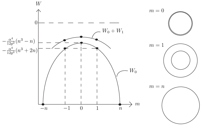
Figure 1: The classical action $W_{0}$ and the one-loop effective action $W_{1}$ as functions of $m$. We also draw the pictures of $2$-concentric fuzzy spheres for $m=0$, $m=1$ case and a single fuzzy sphere ($m=n$) on the right-side.

3.3 Instability of the $U(2)$ gauge theory

In this subsection we analyze the instability of the $U(2)$ gauge theory, the 2-coincident fuzzy spheres of $m=0$, along the zero-modes explained in the previous subsection. We also consider the decay process from this configuration to the TP monopole configuration of $|m|=1$.

In order to see how the 2-coincident fuzzy spheres ($m=0$) decay, we consider the zero-mode directions around this configuration. As we mentioned after (3.8) there are 4 zero-modes, one of which is $A_{i}\sim{\mathbb{1}}_{2n}$, the total translation, and should be neglected due to the tracelessness condition imposed on the matrices $A_{i}$. We thus consider the following background

$$X_{i}=L_{i}^{(n)}\otimes{\mathbb{1}}_{2}+h_{i}^{a}{\mathbb{1}}_{n}\otimes\tau^{a}.$$ (3.14)

The classical action can be obtained by inserting (3.14) into (3.1), and becomes

$$W_{0} = -\frac{\alpha^{4}}{12g^{2}}\bigl{(}n^{3}-n\bigr{)}$$ (3.15)

$$+\frac{\alpha^{4}}{g^{2}}n\left[2\{(h_{i}^{a}h_{i}^{a})^{2}-(h_{i}^{a}h_{j}^{a})^{2}\}-8\det(h_{i}^{a})\right],$$

which has the third and fourth order terms in $h_{i}^{a}$. Since the third order term $-8\det(h_{i}^{a})$ becomes minimum in the direction of $h_{i}^{a}\propto\delta_{ia}$, the two-coincident fuzzy spheres decay into this direction. We also show in appendix B that (3.15) takes an absolute minimum at $h_{i}^{a}=\frac{1}{2}\delta_{ia}$, which is nothing but the TP monopole configuration. Therefore we infer that the 2-coincident fuzzy spheres decay into the TP monopole configuration along the path

$$X_{i}=L_{i}^{(n)}\otimes{\mathbb{1}}_{2}+h{\mathbb{1}}_{n}\otimes\frac{\tau^{i}}{2}$$ (3.16)

from $h=0$ to $h=1$.

Next we evaluate the one-loop correction around the background (3.14). The one-loop effective action can be obtained by inserting (3.14) into (A.8),

$$W_{1} = \frac{1}{2}{\cal T}r\ \hbox{tr}^{\prime}\log\left[({\tilde{X}}_{k})^{2}\delta_{ij}-2i\epsilon_{ijk}h_{k}^{a}{\tilde{\tau}}^{a}+4ih_{i}^{a}h_{j}^{b}\epsilon_{abc}{\tilde{\tau}}^{c}\right]$$ (3.17)

$$-{\cal T}r\log\left[({\tilde{X}}_{k})^{2}\right],$$

where ${\tilde{X}}_{i}$ and ${\tilde{\tau}}_{i}$ are adjoint operators which act on a hermitian matrix $M$ as

$${\tilde{X}}_{i}M = [L_{i}^{(n)}\otimes{\mathbb{1}}_{2}+h_{i}^{a}{\mathbb{1}}_{n}\otimes\tau^{a},M],$$ (3.18)

$${\tilde{\tau}}_{i}M = [\tau_{i},M].$$ (3.19)

Up to the second order of the perturbative expansion in $h_{i}^{a}$, the one-loop effective action becomes

$$W_{1} = 2\sum_{l=1}^{n-1}(2l+1)\log\left[l(l+1)\right]$$ (3.20)

$$+(h_{i}^{a})^{2}\left[\frac{4}{3}\sum_{l=1}^{n-1}\frac{2l+1}{l(l+1)}-16\sum_{l=1}^{n-1}\frac{2l+1}{(l(l+1))^{2}}\right],$$

where we did not include the zero-modes ($l=0$) since they are collective modes and should be treated separately. The coefficient of $(h_{i}^{a})^{2}$ changes its sign from negative to positive at $n=374$, and at large $n$ limit,

$$W_{1} \simeq 2\bigl{[}n(n-1)\bigl{(}\log n(n-1)-1\bigr{)}-2(\log 2-1)\bigr{]}$$ (3.21)

$$+(h_{i}^{a})^{2}\left[\frac{4}{3}\bigl{(}\log n(n-1)-\log 2\bigr{)}-16\left(1-\frac{1}{n^{2}}\right)\right].$$

In summary, the configuration of 2-coincident fuzzy spheres has 3 nontrivial zero-modes, which include the decay direction as was seen from the classical action (3.15). Including the one-loop correction, all of the 3 zero-mode directions become unstable for $n\leq 373$, and stable for $n\geq 374$. Thus this configuration becomes metastable for large $n$. Then the transition to the TP monopole configuration must be qualitatively different. However, since the one-loop contribution is like $(\log n)h^{2}$ while the classical contribution is like $-nh^{3}$, the metastability becomes negligible at large $n$ limit. See Figure 2.

We will illustrate this feature by plotting $W_{0}+W_{1}$ along the path (3.16).

$$W_{0}+W_{1} = -\frac{\alpha^{4}}{12g^{2}}\bigl{(}n^{3}-n\bigr{)}+2\sum_{l=1}^{n-1}(2l+1)\log\left[l(l+1)\right]$$ (3.22)

$$+V_{0}(h)+V_{1}(h),$$

where

$$V_{0}(h) = \frac{\alpha^{4}n}{g^{2}}\Bigl{(}\frac{3}{4}h^{4}-h^{3}\Bigr{)},$$ (3.23)

$$V_{1}(h) = \biggl{[}\sum_{l=1}^{n-1}\frac{2l+1}{l(l+1)}-\!12\Bigl{(}1\!-\!\frac{1}{n^{2}}\Bigr{)}\!\biggr{]}h^{2}.$$ (3.24)

In Figure 2 we plot the classical potential $V_{0}(h)$ in (a), the one-loop effective potential $V_{0}(h)+V_{1}(h)$ for small values of $n$ in (b), and for large values of $n$ in (c).

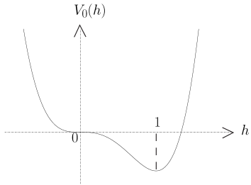
(a) The classical potential $V_{0}$

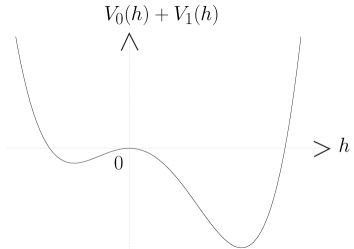
(b) $V_{0}+V_{1}$ for small $n$

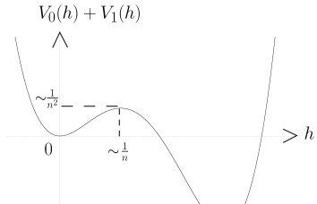
(c) $V_{0}+V_{1}$ for large $n$

Figure 2: (a)The classical potential is flat at $h=0$ and takes a minimum value at $h=1$. (b)The one-loop potential is unstable at $h=0$ for small values of $n$. (c)The one-loop potential is metastable at $h=0$ for large values of $n$.

3.4 Instability of the TP monopole configuration

In the previous subsection we analyzed the transition from the $U(2)$ gauge theory to the TP monopole configuration. As we saw in subsection 3.2, the TP monopole configuration is not stable and decays into the configuration of larger $|m|$. We analyze the instability of the TP monopole in this subsection. To see how the TP monopole configuration decays, we consider the zero-mode directions around this configuration. As we mentioned after (3.8) there are 2 zero-modes, one of which is $A_{i}\sim{\mathbb{1}}_{2n}$, the total translation, and should be neglected. Thus we consider the following background

$$X_{i}=\left(\begin{array}[]{cc}L_{i}^{(n+1)}&\\ &L_{i}^{(n-1)}\end{array}\right)+h_{i}\left(\begin{array}[]{cc}\frac{n-1}{n}{\mathbb{1}}_{n+1}&\\ &-\frac{n+1}{n}{\mathbb{1}}_{n-1}\end{array}\right).$$ (3.25)

The classical action is obtained by inserting (3.25) into (3.1), and becomes

$$W_{0}=-\frac{\alpha^{4}}{12g^{2}}\bigl{(}n^{3}+2n\bigr{)}.$$ (3.26)

Note that this direction is flat not only in the second order but in all orders in $h_{i}$. Thus we have to find the direction along which the TP monopole configuration decays, including the non-zero-modes. It is an interesting study to find such a direction that the potential along the path $h$ has the form like

$$V_{0}(h)\sim n(h^{2}-h^{3}),$$ (3.27)

and the path connects the TP monopole configuration ($|m|=1$) to the configuration of $|m|=2$. In any case, the TP monopole configuration must be metastable classically.

We now evaluate the one-loop effective action around the background (3.25). By inserting it into (A.8), we obtain

$$W_{1} = \frac{1}{2}{\cal T}r\ \hbox{tr}^{\prime}\log\bigl{[}({\tilde{X}}_{k})^{2}\delta_{ij}-2i\epsilon_{ijk}{\tilde{H}}_{k}\bigr{]}$$ (3.28)

$$-{\cal T}r\log\bigl{(}({\tilde{X}}_{k})^{2}\bigr{)},$$

where ${\tilde{X}}_{i}$ and ${\tilde{H}}_{i}$ are adjoint operators which act on a hermitian matrix $M$ as

$${\tilde{X}}_{i}M = \Biggl{[}\biggl{(}\begin{array}[]{cc}L_{i}^{(n+1)}&\\ &L_{i}^{(n-1)}\end{array}\biggr{)}+h_{i}\biggl{(}\begin{array}[]{cc}\frac{n-1}{n}{\mathbb{1}}_{n+1}&\\ &-\frac{n+1}{n}{\mathbb{1}}_{n-1}\end{array}\biggr{)},M\Biggr{]},$$ (3.33)

$${\tilde{H}}_{i}M = \Biggl{[}h_{i}\biggl{(}\begin{array}[]{cc}\frac{n-1}{n}{\mathbb{1}}_{n+1}&\\ &-\frac{n+1}{n}{\mathbb{1}}_{n-1}\end{array}\biggr{)},M\Biggr{]}.$$ (3.36)

Up to the second order of the perturbation in $h_{i}$,

$$W_{1} = \frac{1}{2}\biggl{(}\sum_{l=1}^{n}+\sum_{l=1}^{n-2}+2\sum_{l=1}^{n-1}\biggr{)}(2l+1)\log\left[\,l(l+1)\right]$$ (3.37)

$$+(h_{i})^{2}\Biggl{[}\frac{4}{3}\sum_{l=1}^{n-1}\frac{2l+1}{l(l+1)}-16\sum_{l=1}^{n-1}\frac{2l+1}{(l(l+1))^{2}}\Biggr{]},$$

where again we have subtracted the zero-modes since they are collective modes and should be treated separately. The coefficient of $(h_{i})^{2}$ changes its sign from negative to positive at $n=374$, and becomes $8/3\log n$ at large $n$ limit. Therefore, along this direction, the TP monopole configuration is unstable for small $n$, while stable for large $n$.

As for the decay from the TP configuration, we must consider other directions. As we mentioned in (3.27), the TP configuration is metastable even at the classical level. The quantum corrections of the order of $(\log n)h^{2}$ will not change the qualitative feature of the classical metastability. It is plausible that all of the monopole configurations of $|m|\geq 1$ have the same property, since they also have only one nontrivial zero-mode.

4 Conclusion and Discussion

In this paper we presented a dynamical mechanism for an index generation through the spontaneous symmetry breaking: $U(2)\simeq SU(2)\times U(1)\rightarrow U(1)\times U(1)$, by showing that the monopole configurations with the nontrivial topological charges are stabler than the $U(2)$ gauge theory without any condensation on the fuzzy 2-sphere, though it finally decays to a single fuzzy 2-sphere whose effective theory is the $U(1)$ gauge theory on the fuzzy 2-sphere. The final state is geometrically different from the initial state, two-coincident fuzzy spheres. Nevertheless, we expect that such a mechanism of the dynamical generation of an index as studied in this paper would be useful to realize chiral fermions dynamically by compactifying extra-dimensional spaces with a nontrivial index in some more realistic matrix models.

We first analyzed the instability of the general monopole configurations (2.28) in the Yang-Mills-Chern-Simons matrix model. The classical action for these configurations monotonously decreases as the difference of the sizes of the two matrices, $|m|$, increases (see Figure 1). Thus the $U(2)$ gauge theory, the 2-coincident spheres of $m=0$, is unstable and decays to the TP monopole configuration of $|m|=1$. Repeating such transitions, it cascades to the $U(1)$ gauge theory, the single sphere of $|m|=n$. These properties do not change even after we take into consideration the quantum corrections. Namely, the vacuum structure is determined classically.

We then analyzed the instability of the $U(2)$ gauge theory ($m=0$), in detail. This configuration has 3 nontrivial zero-modes, which includes the direction along which it decays to the TP monopole ($|m|=1$). Including the one-loop correction, all of the 3 zero-mode directions become unstable for $n\leq 373$, and stable for $n\geq 374$. Thus the $U(2)$ gauge theory becomes metastable for large $n$. Then the transition to the TP monopole configuration must be qualitatively different: 2nd order like transition for small $n$ and 1st order like for large $n$. However, since the one-loop contribution is like $(\log n)h^{2}$ while the classical contribution is like $-nh^{3}$, the metastability becomes negligible at large $n$ limit.

It will be interesting to study the decay processes from the $U(2)$ gauge theory to the TP monopole configuration in detail. If we introduce an extra time direction and consider the action (3.1) as the potential, we can discuss the instability of the fuzzy sphere in the M(atrix)-theory[41] or the instability observed in the Monte Carlo simulation of the matrix model in [37]. Then we can evaluate the decay rate by using the path (3.16) in some semiclassical method.

We further analyzed the instability of the TP monopole configuration ($|m|=1$). This configuration has one nontrivial zero-mode, which is a flat direction classically. The one-loop quantum correction makes it unstable for small $n$ and stable for large $n$. As for the decay we have to consider other directions, which include the non-zero-modes. Thus the TP monopole configuration must be metastable even at the classical level, and quantum corrections will not change this property. It is plausible that all of the configurations of $|m|\geq 1$ have this property since they have only one zero-mode.

It is interesting to find the decay path from the TP configuration of $|m|=1$ to the one of $|m|=2$, and the path from $|m|=2$ to $|m|=3$, and so on, and check the above mentioned conjecture. It is also interesting to clarify the explicit form of the configuration of the general monopoles of $|m|\geq 2$, as we did for $|m|=1$ in [28].

Another issue is to study topologically nontrivial configurations in other NC geometries than the fuzzy 2-sphere and present a mechanism for the dynamical generation of an index on general NC geometries. We might be able to use this mechanism in the matrix models for the critical string theories like [1], and realize the chiral gauge theory in our four-dimensional space-time.

Appendix A The one-loop effective action

Here we give the calculation of the one-loop effective action in the background-field method. We consider backgrounds $X_{i}$ and fluctuations around it, $\tilde{A}_{i}$:

$$A_{i}=X_{i}+\tilde{A}_{i}.$$ (A.1)

We add to the action (3.1) the gauge fixing term and the ghost term:

$$S_{\rm g.f.} = -\frac{1}{g^{2}}\hbox{tr}[X_{i},A_{i}]^{2}\ ,$$ (A.2)

$$S_{\rm ghost} = -\frac{1}{g^{2}}\hbox{tr}\left([X_{i},\bar{c}][A_{i},c]\right)\ ,$$ (A.3)

where $c$ and $\bar{c}$ are the ghost and anti-ghost fields, respectively.

We then expand the action (3.1) up to the second order in the fluctuations:

$$S_{\rm total} = S[X_{i}]+S_{2}\ ,$$ (A.4)

$$S_{2} = \frac{1}{2g^{2}}\hbox{tr}\left(\tilde{A}_{i}[X_{k},[X_{k},\tilde{A}_{i}]]-2\bigl{(}[X_{i},X_{j}]-i\epsilon_{ijk}X_{k}\bigr{)}[\tilde{A}_{i},\tilde{A}_{j}]\right)$$ (A.5)

$$+\frac{1}{g^{2}}\hbox{tr}\Bigl{(}\bar{c}\,[X_{k},[X_{k},c]]\Bigr{)}$$

$$= \frac{1}{2g^{2}}\hbox{tr}\left(\tilde{A}_{i}\bigl{[}({\tilde{X}}_{k})^{2}\delta_{ij}+2\bigl{(}[{\tilde{X}}_{i},{\tilde{X}}_{j}]-i\epsilon_{ijk}{\tilde{X}}_{k}\bigr{)}\bigr{]}\tilde{A}_{j}\right)$$

$$+\frac{1}{g^{2}}\hbox{tr}\Bigl{(}\bar{c}\ ({\tilde{X}}_{k})^{2}c\Bigr{)},$$

where in the last step we introduced adjoint operators,

$${\tilde{X}}_{i}M = [X_{i},M],$$ (A.6)

$$\bigl{(}[{\tilde{X}}_{i},{\tilde{X}}_{j}]-i\epsilon_{ijk}{\tilde{X}}_{k}\bigr{)}M = [\bigl{(}[X_{i},X_{j}]-i\epsilon_{ijk}X_{k}\bigr{)},M].$$ (A.7)

Note that we drop the linear terms in $\tilde{A}_{i}$ by hand in the background-field method.

The one-loop effective action $W_{1}$ is obtained as

$$W_{1} = -\log\int d\tilde{A}dcd\bar{c}\ e^{-S_{2}}$$ (A.8)

$$= \frac{1}{2}{\cal T}r\ \hbox{tr}^{\prime}\log\bigl{[}({\tilde{X}}_{k})^{2}\delta_{ij}+2\bigl{(}[{\tilde{X}}_{i},{\tilde{X}}_{j}]-i\alpha\epsilon_{ijk}{\tilde{X}}_{k}\bigr{)}\bigr{]}$$

$$-{\cal T}r\log\bigl{[}({\tilde{X}}_{k})^{2}\bigr{]},$$

where ${\cal T}r$ is a trace of operators acting on matrices, and $\hbox{tr}^{\prime}$ is the trace over the space-time indices $i$ and $j$.

Appendix B Analysis of the potential (3.15)

In this appendix we show that the potential (3.15) has the absolute minimum at $h_{i}^{a}=\frac{1}{2}\delta_{ia}$, which is nothing but the TP monopole configuration. The potential (3.15) can be written as

$$V(H)=2[(\hbox{tr}H^{T}H)^{2}-\hbox{tr}(H^{T}HH^{T}H)]-8\det(H),$$ (B.1)

where $(H)_{ia}=h_{i}^{a}$. Introducing $M=H^{T}H$,

$$V(H) = 2[(\hbox{tr}M)^{2}-\hbox{tr}(M^{2})]\mp 8\sqrt{\det M}$$ (B.2)

$$= 2\Bigl{[}\Bigl{(}\sum\nolimits_{i=1}^{3}x_{i}\Bigr{)}^{2}-\sum\nolimits_{i=1}^{3}x_{i}^{2}\Bigr{]}\mp 8\sqrt{\prod_{i}x_{i}}$$

$$= 4(x_{1}x_{2}+x_{2}x_{3}+x_{3}x_{1})\mp 8\sqrt{x_{1}x_{2}x_{3}}\ ,$$

up to the overall coefficient. Here $x_{1},x_{2},x_{3}$ are the eigenvalues of $M$. Fixing the value of $x_{1}x_{2}x_{3}$, the first term in eq.(B.2) has a lower bound as

$$x_{1}x_{2}+x_{2}x_{3}+x_{3}x_{1} = (x_{1}x_{2}x_{3})\left(\frac{1}{x_{1}}+\frac{1}{x_{2}}+\frac{1}{x_{3}}\right)$$ (B.3)

$$\geq 3(x_{1}x_{2}x_{3})\left(\frac{1}{x_{1}x_{2}x_{3}}\right)^{\frac{1}{3}}$$

$$= 3(x_{1}x_{2}x_{3})^{\frac{2}{3}},$$

where in the second inequality the equality is satisfied when $x_{1}=x_{2}=x_{3}\equiv y^{2}$. In this case $V(H)$ is given by

$$V(H) = 12y^{4}-8y^{3}$$ (B.4)

$$\geq -\frac{1}{4},$$

where in the second line equality is satisfied when $y=\frac{1}{2}$.

Therefore the minimal point $V(H)=-1/4$ is satisfied at $h_{i}^{a}=\frac{1}{2}\delta_{i}^{a}$ up to $SU(2)$ rotation. Thus $W_{0}$ in (3.15) is minimized at the TP monopole configuration under the restriction on possible directions to move in the configuration space as in eq(3.14).

References

- [1] N. Ishibashi, H. Kawai, Y. Kitazawa and A. Tsuchiya, Nucl. Phys. B 498, 467 (1997) [arXiv:hep-th/9612115]. For a review, see H. Aoki, S. Iso, H. Kawai, Y. Kitazawa, A. Tsuchiya and T. Tada, Prog. Theor. Phys. Suppl. 134, 47 (1999) [arXiv:hep-th/9908038].
- [2] A. Connes, Noncommutative geometry, Academic Press, 1990.
- [3] A. Connes, M. R. Douglas and A. Schwarz, JHEP 9802, 003 (1998) [arXiv:hep-th/9711162].
- [4] H. Aoki, N. Ishibashi, S. Iso, H. Kawai, Y. Kitazawa and T. Tada, Nucl. Phys. B 565, 176 (2000) [arXiv:hep-th/9908141].
- [5] H. Grosse, C. Klimcik and P. Presnajder, geometry,” Commun. Math. Phys. 178, 507 (1996) [arXiv:hep-th/9510083]; S. Baez, A. P. Balachandran, B. Ydri and S. Vaidya, Commun. Math. Phys. 208, 787 (2000) [arXiv:hep-th/9811169]; G. Landi, J. Geom. Phys. 37, 47 (2001) [arXiv:math-ph/9905014].
- [6] A. P. Balachandran and S. Vaidya, Int. J. Mod. Phys. A 16, 17 (2001) [arXiv:hep-th/9910129].
- [7] P. Valtancoli, Mod. Phys. Lett. A 16, 639 (2001) [arXiv:hep-th/0101189].
- [8] H. Steinacker, Nucl. Phys. B 679, 66 (2004) [arXiv:hep-th/0307075].
- [9] D. Karabali, V. P. Nair and A. P. Polychronakos, Nucl. Phys. B 627, 565 (2002) [arXiv:hep-th/0111249].
- [10] U. Carow-Watamura, H. Steinacker and S. Watamura, arXiv:hep-th/0404130.
- [11] P. H. Ginsparg and K. G. Wilson, Phys. Rev. D 25, 2649 (1982).
- [12] M. Lüscher, Phys. Lett. B 428, 342 (1998) [arXiv:hep-lat/9802011].
- [13] F. Niedermayer, Nucl. Phys. Proc. Suppl. 73, 105 (1999) [arXiv:hep-lat/9810026].
- [14] P. Hasenfratz, Nucl. Phys. Proc. Suppl. 63, 53 (1998) [arXiv:hep-lat/9709110]; P. Hasenfratz, V. Laliena and F. Niedermayer, Phys. Lett. B 427, 125 (1998) [arXiv:hep-lat/9801021].
- [15] H. Neuberger, Phys. Lett. B 417, 141 (1998) [arXiv:hep-lat/9707022]; Phys. Rev. D 57, 5417 (1998) [arXiv:hep-lat/9710089]; Phys. Lett. B 427, 353 (1998) [arXiv:hep-lat/9801031].
- [16] H. Aoki, S. Iso and K. Nagao, Phys. Rev. D 67, 085005 (2003) [arXiv:hep-th/0209223]. For a very short review, see K. Nagao, Nucl. Phys. Proc. Suppl. 129, 501 (2004) [arXiv:hep-th/0309153].
- [17] J. Madore, Class. Quant. Grav. 9, 69 (1992).
- [18] U. Carow-Watamura and S. Watamura, Commun. Math. Phys. 183, 365 (1997) [arXiv:hep-th/9605003]; Commun. Math. Phys. 212, 395 (2000) [arXiv:hep-th/9801195].
- [19] H. Grosse and J. Madore, Phys. Lett. B 283, 218 (1992); H. Grosse and P. Presnajder, Lett. Math. Phys. 33, 171 (1995); H. Grosse, C. Klimcik and P. Presnajder, Commun. Math. Phys. 185, 155 (1997) [arXiv:hep-th/9507074]; arXiv:hep-th/9603071.
- [20] S. Iso, Y. Kimura, K. Tanaka and K. Wakatsuki, Nucl. Phys. B 604, 121 (2001) [arXiv:hep-th/0101102].
- [21] H. Grosse and P. Presnajder, arXiv:hep-th/9805085; Lett. Math. Phys. 46, 61 (1998).
- [22] P. Presnajder, J. Math. Phys. 41, 2789 (2000) [arXiv:hep-th/9912050].
- [23] H. Aoki, S. Iso and K. Nagao, Phys. Rev. D 67, 065018 (2003) [arXiv:hep-th/0209137].
- [24] A. P. Balachandran, T. R. Govindarajan and B. Ydri, Mod. Phys. Lett. A 15, 1279 (2000) [arXiv:hep-th/9911087].
- [25] A. P. Balachandran, T. R. Govindarajan and B. Ydri, hep-th/0006216.
- [26] B. Ydri, JHEP 0308, 046 (2003) [arXiv:hep-th/0211209].
- [27] A. P. Balachandran and G. Immirzi, Phys. Rev. D 68, 065023 (2003) [arXiv:hep-th/0301242].
- [28] H. Aoki, S. Iso and K. Nagao, Nucl. Phys. B 684, 162 (2004) [arXiv:hep-th/0312199].
- [29] J. Nishimura and M. A. Vazquez-Mozo, JHEP 0108, 033 (2001) [arXiv:hep-th/0107110].
- [30] S. Iso and K. Nagao, Prog. Theor. Phys. 109, 1017 (2003) [arXiv:hep-th/0212284].
- [31] T. Fujiwara, K. Nagao and H. Suzuki, JHEP 0209, 025 (2002) [arXiv:hep-lat/0208057].
- [32] J. Nishimura and M. A. Vazquez-Mozo, JHEP 0301, 075 (2003) [arXiv:hep-lat/0210017].
- [33] A. Y. Alekseev, A. Recknagel and V. Schomerus, JHEP 0005, 010 (2000) [arXiv:hep-th/0003187].
- [34] S. Bal and H. Takata, Int. J. Mod. Phys. A 17, 2445 (2002) [arXiv:hep-th/0108002].
- [35] P. Valtancoli, Int. J. Mod. Phys. A 18, 967 (2003) [arXiv:hep-th/0206075].
- [36] T. A. Imai, Y. Kitazawa, Y. Takayama and D. Tomino, Nucl. Phys. B 665, 520 (2003) [arXiv:hep-th/0303120].
- [37] T. Azuma, S. Bal, K. Nagao and J. Nishimura, JHEP 0405, 005 (2004) [arXiv:hep-th/0401038].
- [38] P. Castro-Villarreal, R. Delgadillo-Blando and B. Ydri, Nucl. Phys. B 704, 111 (2005) [arXiv:hep-th/0405201].
- [39] T. Azuma, S. Bal, K. Nagao and J. Nishimura, arXiv:hep-th/0405277.
- [40] T. Azuma, K. Nagao and J. Nishimura, arXiv:hep-th/0410263.
- [41] T. Banks, W. Fischler, S. H. Shenker and L. Susskind, Phys. Rev. D 55, 5112 (1997) [arXiv:hep-th/9610043].