The nonsingular brane solutions via the Darboux transformation

Abstract

We consider the Darboux transformation as a method of construction of exact nonsingular solutions describing the three-dimensional brane that interacts with five-dimensional gravity and the bulk scalar field. To make it work, the five-dimensional Einstein’s equations and the Israel’s conditions are being reduced to the Schrödinger equation with the jump-like potential and the wave functions sewing conditions in jump point correspondingly. We show further that it is always possible to choose the functions in Crum’s determinants in such way, that the five-dimensional Ricci scalar $R$ will always be finite both on brane and in bulk. The new exact solutions being the generalizations of the model with the odd superpotential are presented. Described formalism is also appliable to the cases of more realistic branes with cosmological expansion. As an example, via the usage of the simple orbifold model ($S_{1}/{\mathbb{Z}}_{2}$) and one-time Darboux transformation we construct the models where the cosmological constant on the visible brane is exponentially small.

I Introduction

In article Flanagan , there have been considered an interesting model, which describes the set of parallel 3-branes, all of them being imbedded in five-dimensional bulk, filled with the gravitation and the scalar field. The action of set is expressed as:

$$\begin{array}[]{c}S=\int d^{4}xdy\sqrt{\mid g\mid}\left(\frac{1}{2}R-\frac{(\nabla\phi^{2})}{2}-V(\phi)\right)-\\ \sum_{b}\int_{y_{b}}d^{4}x\sqrt{\mid{\tilde{g}}^{b}\mid}\sigma_{b}(\phi),\end{array}$$ (1)

where $(x^{\mu},y)$ and $0\leq\mu\leq 3$ are the five-dimensional coordinates; brane number $b$ is located at $y=y_{b}$; $g_{ab}$ is the 5-D metric, and ${\tilde{g}}^{b}_{\mu\nu}$ is the metric, induced on the $b$th brane. (Note that it is written in special system of units, where the gravitational constant $\kappa=1$ and speed of light $c=1$.) The tension on the $b$th brane is named $\sigma_{b}$, and the potential $V(\phi)$ is considered to be a function of the bulk scalar field $\phi=\phi(y)$. The field equations follows from the (1) by the procedure of variation; their solution is assumed to have a form (Flanagan ):

$$ds^{2}=dy^{2}+A(y)\left(-dt^{2}+e^{2Ht}\delta_{ik}dx^{i}dx^{k}\right),$$ (2)

where $A(y)$ is a sought warp factor, and $H$=const is a Hubble parameter. If $H=0$ on the brane, the brane will be the stationary one, and if $H>0$, then the brane will be expanding in the de Sitter regime uskor .

The (1) leads to system of differential equations, that, in turn, can be rewritten in ”supersymmetric” style by introduction of the superpotential $W(\phi)$, being defined by the ${\dot{\phi}}\equiv W^{\prime}(\phi)/2$ relation, where the dot denotes the derivative in $y$, and the prime – the derivative in $\phi$. In case of $H=0$ there exists following equation

$$V(\phi)=W^{\prime 2}/8-W^{2}/6.$$ (3)

Upon usage of this equation, the authors of Flanagan have suggested a simple way of obtaining of exact solutions of the field equations (see also RS , TW for further details). Their approach can be expressed in following steps:
(i) Choosing convenient $V(\phi)$ and $W(\phi)$, making sure that the equation (3) with these new values still holds true;
(ii) Integration of equation ${\dot{\phi}}\equiv W^{\prime}(\phi)/2$, in order to receive the relation $\phi=\phi(y)$;
(iii) When $H=0$ there exists the relation ${\dot{A}}(y)/A(y)=-W(\phi(y))/3$. Hence, substitution of the obtained function for $\phi(y)$ in explicit equation for $W(\phi)$ and further integration results in the sought warp factor $A(y)$.

From this point, the famous solutions RS (Randall-Sundrum) turns out to be just a case $W(\phi)=\pm a^{2}={\rm const}$. Authors Flanagan have also considered the models with even ($W(\phi)=\pm\left(a^{2}-b\phi^{2}\right)$), odd ($W(\phi)=\pm 2b^{2}\phi$) and exponential ($W(\phi)=2a{\rm e}^{-k\phi}$) potentials (the even superpotentials had been previously discussed in DFGK , and the odd ones had been introduced in kaku ).

The major advantage of the described method lies in it’s simplicity. For example, it allows an easy construction of nonsingular solutions (see also kaku ). Lets consider the case of one brane, localized in $y=y_{0}$. From the equation ${\dot{\phi}}\equiv W^{\prime}(\phi)/2$ it is possible to express $y$ as a function of the field variable $\phi$:

$$y(\phi)=y_{0}+\int_{\phi_{0}}^{\phi}\frac{d{\tilde{\phi}}}{W^{\prime}({\tilde{\phi}})},$$ (4)

where $\phi_{0}=\phi(y_{0})$ is a value of a scalar field on brane. It follows from the (4) that the very existence of zeros of the function $W^{\prime}(\phi)$ ($\phi=\phi^{\pm}={\rm const}$, $\mid\phi^{\pm}\mid<\infty$) is leading to the divergences of the integral. In another words, $\phi\to\phi^{\pm}$ when $y\to\pm\infty$. What it means, is that if we choose the superpotential as having at least two zeros at both $\phi>\phi_{0}$ and $\phi<\phi_{0}$ where $W^{\prime}$ is vanishing fast enough (for example $W^{\prime}(\phi)\sim\mid\phi-\phi^{\pm}\mid^{k}$, with $k\geq 1$, and $\phi\to\phi^{\pm}$), then the field $\phi$ remains finite throughout all the $bulk$ space. On the other hand, the case of $H=0$ allows to express the Ricci scalar via the superpotential and its derivative in the form:

$$R(\phi)=2(W^{\prime}(\phi))^{2}/3-5W^{2}(\phi)/9,$$ (5)

thus, showing the finiteness of the scalar curvature for the aforementioned nonsingular superpotential for every $y$. The particular examples of the nonsingular solutions for even, odd and exponential superpotentials can all be found in Flanagan . It also contains the generalization of this technique for the non-stationary branes ($H\neq 0$) and a brief discussion touching the possible usages of the method in solving such a well known problems as the problem of cosmological constant’s smallness and the hierarchy problem.

However, in spite of all the strong points, this method does have its apparent weaknesses, the primal one being its ”phenomenological” nature - the fact, that each physically consistent (i.e. leading to the reasonable $\phi(y)$ and $A(y)$) superpotential $W(\phi)$ can only be obtained by ”guessing”. Although all simple examples, considered in Flanagan were not too hard ”to guess” and they do lead to sensible cosmological models, it would not necessarily be that easy, whenever we try the more difficult (and hence, more realistic) $W(\phi)$. These reasonings lead us to principal question: does there exist such procedure of (1)’s nonsingular solutions construction, which is both mathematically simple and regular? In this work we give the positive answer for this question and introduce the new method, which satisfies both of the conditions.

The general idea of our approach can be formulated as follows: the supersymmetric link between $V(\phi)$ and $W(\phi)$ is a typical one for the supersymmetric quantum mechanics (SSQM). In turn, SSQM is realizable through the usage of Darboux transformation (DT) for the Schrödinger equation Salle , ABI , and that allows us to construct the integrable nonsingular potentials - providing that all the prop functions of Crum’s determinants do have the intermittent zeros Salle , Adler . So, it seems to be only natural trying to write the DT for the field equations directly, and then using them as a source of a new exact solutions. An existence of quite simple algebraic connections between the Ricci scalar and the superpotential (5) notes that construction of nonsingular potentials in SSQM via the right DT application will also aid in development of the systematical procedure of construction of the nonsingular solutions ($R\neq\infty$) in the brane theory, which, by that means, will turn out to be a regular one - as distinct from the ”phenomenological approach” of Flanagan . In particular, the DT method, if applied to just a single exactly solvable potential, grants us the infinite number of an exact nonsingular solutions, with the mentioned potential being a ”fuse” in all those solutions construction. For example, in this work we’ll take the RS for the role of such a fuse solution. Another interesting way of the DT usage is a construction of the chains of discrete symmetries and the further inquiries of their closures. Such a technique allows getting the new exact solutions, which are manifested through the Painlevé transcendents and the higher extensions.

The article has the following structure. Next paragraph is dedicated to the Darboux transformations and to their compatibility with the Israels jump conditions at the brane Israel . In third paragraph we’ll present some new exact solutions, received by one-time Darboux dressing of the RS solutions. Double DT, the importance of the shape-invariance and the dressing chains are all examined in the fourth paragraph. In particular, it will be shown, that even, odd and exponential superpotentials, discussed in work Flanagan are just the examples of the shape-invariants with regard to DT potentials. In the same section we’ll show the exact solutions, that serve as the generalizations of the model with the odd superpotential (here we include the solutions expressed via the fourth Painlevé transcendent). In paragraph 5 we’ll describe the construction of an exact solutions for the non-stationary branes, made with the usage of DT and will discuss the nascent difficulties. Here we’ll consider both noncompact and compact spacetimes. In the last case, using the simple orbifold model ($S_{1}/{\mathbb{Z}}_{2}$) and one-time Darboux transformation we’ll construct the models with two branes where the cosmological constant on the one of them (visible brane) will be exponentially small. Also, we’ll outline the new approach (called Green function method) which allows to construct solutions both in stationary and non-stationary cases. Finally, the six paragraph is an overall conclusion.

II Darboux transformations and jump conditions

If $H=0$ and $u\equiv{\dot{A}}/A$, then from the (1) and (2) we get the following set of equations Flanagan :

$${\dot{u}}=-\frac{2{\dot{\phi}}^{2}}{3}-\frac{2}{3}\sum_{b}\sigma_{b}(\phi)\delta(y-y_{b}),\qquad u^{2}=\frac{{\dot{\phi}}^{2}}{3}-\frac{2}{3}V(\phi).$$ (6)

Third equation has the form

$$\ddot{\phi}+2u\dot{\phi}=\frac{\partial V(\phi)}{\partial\phi}+\sum_{b}\frac{\partial\sigma_{b}(\phi)}{\partial\phi}\delta(y-y_{b}),$$

and is not independent, because it can be received from the set (6). In case of the single brane, located at $y=0$, we get $\sigma(\phi(y))\delta(y)=\sigma_{0}\delta(y)$, where $\sigma_{0}=\sigma(\phi(0))$ (supposing $\phi(0)\neq 0$). It is easy to check, that the function $A^{2}(y)$ satisfies the Schrödinger equation

$$\left(\frac{d^{2}}{dy^{2}}+\frac{8}{3}V(\phi(y))+\beta\delta(y)\right)A^{2}(y)=0,$$ (7)

where $\beta=4\sigma_{0}/3$. Now lets define the spectral problem

$$\ddot{\psi}=\left(v(y)-\beta\delta(y)-\lambda\right)\psi,$$ (8)

where $\psi=\psi(y;\lambda)$ and $v(y)$ is a certain potential which will be further refereed to as a quantum-mechanical potential, or QM-potential. Lets assume, that it is possible to solve the equation (8) formally (i.e., obtaining among others some ”non-physical” solutions which do not belong to $L^{2}$) for some QM-potential $v(y)$ and all $\lambda\in\mathbb{R}$. Lets then suppose that for some values of the spectral parameter $\lambda$ (say, $\lambda=\lambda_{0}$) the solutions of the (8) will be strictly positive: $\psi(y;\lambda_{0})>0$. In this case we can conclude that function $A(y;\lambda_{0})=\sqrt{\psi(y;\lambda_{0})}$ is the solution of the (7) with potential

$$V(\phi(y))=\frac{3}{8}\left(\lambda_{0}-v(y)\right).$$ (9)

Therefore, the equation (8) can, in fact, be considered as the producer of exact solutions of the (7). Substituting $A(y)$ and $V(\phi(y))$, obtained from the (8), in (6) we’ll find out $\phi=\phi(y)$. In this point there can be raised the question: what solutions can be named the physically sensible one? More precisely, what can be said about the solutions with ${\dot{\phi}}^{2}<0$?

Nota Bene 1. Recently the great deal of interest has been drawn to those very specifical cosmological models, which admits the violation of the dominant-energy condition 1 . Such models often presuppose that the ”dark energy” has so-called phantom component 2 , which should be described by some scalar field with the negative kinetic term. Quantum theory of those fields has been considered in 3 (this work also has an almost complete bibliography of a subject). As a general result of this investigations we can point out the following indication: apparently such fields fails to be consistently considered as a fundamental objects. But nevertheless, we can’t totally exclude the probability that the Lagrangians with the negative kinetic terms will somehow appear in a role of effective models. For example, similar terms appear in some models of supergravity 4 and in the gravity theories with highest derivatives 5 . Finally, the ”phantom energy” in the brane theory was considered in 7 . However, despite of all the above said, we will not further consider the phantom component. In other words, we shall suppose that ${\dot{\phi}}^{2}>0$ during the rest of this paper.

For specificity, we’ll further assume the following condition for the potential $v(y)$:

$${v(y)={\rm const}+{\tilde{v}}(y),\qquad\int_{-\infty}^{+\infty}dy\,\left(1+|y|\right)|{\tilde{v}}(y)<\infty.}$$ (10)

It is also worth mentioning, that for our further investigation the validity of (10) is not really necessary. We just found it to be convenient to consider the potentials, that are confined within such bounds.

So, lets assume the parameters $\psi(y)$, $v(y)$, $\lambda$ to be already determined. We are going to find the functions $A(y)$, $\phi(y)$ and $V(\phi)$. In order to do this we’ll examine the region located far from the brane to exterminate the $\delta$-function term in the (8) from further considerations. It’s obvious, that the quantity $A(y)$ can only be restored if $\psi(y)$ is nonnegative for all $y$. The only one wave function that both satisfies this condition and belongs to the physical spectrum of Schrödinger equation (8), is a wave function of ground state with $\lambda=\lambda_{{}_{vac}}$. We should also mention, that there exists another possible way to choose the ”good” wave function, namely, to consider the case $\lambda=\lambda_{-1}<\lambda_{{}_{vac}}$. This satisfies the imposed condition, since the (8) indeed admits the always positive solutions $\psi(y;\lambda_{-1})$. These solutions obviously do not belong to the $L_{2}$ space and definitely do not describe the bound states, but the warp factor $A=\sqrt{\psi(y;\lambda_{{}_{1}})}$ will nevertheless be real. However, these solutions result in singularity at infinity: $A\to\infty$ at $y\to\infty$, and therefore the ground state $\psi(y;\lambda_{{}_{vac}})$ is by far the best alternative to $\psi(y;\lambda_{-1})$

It is well known, that DT has a remarkable capacity to enable the engineering of ad hoc potentials with arbitrary finite discrete spectrum, thus it can be consistently considered as a procedure of construction of the system (6)’s exact solutions. We’ll now quickly remind the very essence of DT method Darboux . Let $\psi_{1}=\psi(y;\lambda_{1})$ and $\psi_{2}=\psi(y;\lambda_{2})$ be the two solutions of the equation (8), and let also $\psi_{1}>0$ for every $y$ it is defined on. The $\psi_{1}$ is called the prop function of Darboux transformation. In general, the transformation law is:

$$\begin{array}[]{cc}\displaystyle{\psi_{2}\to\psi_{2}^{(1)}=\frac{{\dot{\psi}_{2}}\psi_{1}-{\dot{\psi}_{1}}\psi_{2}}{\psi_{1}}},\\ \\ \displaystyle{v\to v^{(1)}=v-2\frac{d^{2}}{dy^{2}}\log\psi_{1},\qquad\lambda_{2}\to\lambda_{2}}.\end{array}$$ (11)

Darboux transformation (11) is an isospectral symmetry of equation (8), because the dressed function $\psi_{2}^{(1)}$ is the solution of the dressed equation (8):

$$\ddot{\psi}_{2}^{(1)}=\left(v^{(1)}-\beta^{(1)}\delta(y)-\lambda_{2}\right)\psi_{2}^{(1)},$$

with a new (dressed) potential $v^{(1)}$ but with the same value of $\lambda^{(1)}_{2}=\lambda_{2}$. The transformation law for the prop function is given by the relation (Salle ):

$$\begin{array}[]{c}\psi_{1}\to\psi_{1}^{(1)}=\frac{1}{\psi_{1}}\left(C_{1}+C_{2}\int\psi_{1}^{2}(y)dy\right),\\ \\ \ddot{\psi}_{1}^{(1)}=\left(v^{(1)}-\beta^{(1)}\delta(y)-\lambda_{1}\right)\psi_{1}^{(1)},\end{array}$$ (12)

with arbitrary constants $C_{1,2}$ (and, of course, $\lambda^{(1)}_{1}=\lambda_{1}$). The most interesting part for us here is a ground state of a dressed Hamiltonian. There exist three possibilities.

1) If $\psi_{1}$ is a wave function of a ground state, and $\lambda_{2}$ is an energy of a first excited level, then the new dressed function $\psi^{(1)}_{2}$ will be the wave function of a new Hamiltonian’s ground state ABI . All other values of the discrete spectrum of this Hamiltonian are received by simple obliteration of level $\lambda_{1}$ from the initial spectrum.

2) The prop function $\psi_{1}=\psi_{1}(y;\lambda_{1})$ does not belong to an $L_{2}$, but it doesn’t has any zeros either, and $\psi_{1}\to e^{+p^{2}|y|}$ when $y\to\pm\infty$. In the case, after the DT we’ll get the new Hamiltonian, whose discrete spectrum is just an old one except for the new state $\lambda=\lambda_{1}$ added, thereby being the new ground state. The corresponding wave function $\psi^{(1)}_{1}$ (12) with $C_{2}=0$ becomes the ground state’s wave function bereza .

3) The aforementioned prop function can in fact be represented as a linear superposition of two positive, linearly independent solutions $\psi_{1}^{(\pm)}$ with the following characteristics: $\psi_{1}^{(\pm)}\to 0$ when $y\to\mp\infty$ and $\psi_{1}^{(\pm)}\to e^{+p^{2}|y|}$ when $y\to\pm\infty$. Taking either $\psi_{1}^{(+)}$ or $\psi_{1}^{(-)}$ as a prop function results in creation of a new Hamiltonian, whose discrete spectrum is totally coincides with the initial one bereza .

Our article is dedicated in general to the second case.

As a next step of our consideration we should examine the jump conditions, existing on the brane. These conditions can be written as

$$\psi_{i+}(0)=\psi_{i-}(0)=\psi_{i}(0),\qquad{\dot{\psi}}_{i+}(0)-{\dot{\psi}}_{i-}(0)=-\beta\psi_{i}(0).$$ (13)

where $\psi_{i+}(y)$ and $\psi_{i-}(y)$ are the solutions of Schrödinger equation (8), both with the same potential and eigenvalues, but valid only for positive or negative $y$ correspondingly:

$${\ddot{\psi}}_{i\pm}=\left(v(y)-\beta\delta(y)-\lambda_{i}\right)\psi_{i\pm}.$$ (14)

It is easily verified, that (13) are exactly the same jump conditions as in before-cited article Flanagan :

$$\begin{array}[]{c}u_{+}(0)-u_{-}(0)=\frac{1}{2}\left(\frac{{\dot{\psi}}_{+}(0)}{\psi_{+}(0)}-\frac{{\dot{\psi}}_{-}(0)}{\psi_{-}(0)}\right)=\\ \frac{{\dot{\psi}}_{+}(0)-{\dot{\psi}}_{-}(0)}{2\psi(0)}=-\frac{\beta}{2}=-\frac{2\sigma_{0}}{3},\end{array}$$

being, in essence, the Israel conditions Israel , Rubakov . The next theorem proves, that DT keeps the jump conditions (13) unchanged:

Theorem. If $\psi_{i}(y)=\left\{\psi_{i+}(y>0),\psi_{i-}(y<0)\right\}$ with $i=1,2$ are solutions of (14), satisfying the (13) and if $\psi_{1}=\left\{\psi_{{}_{1+}},\psi_{{}_{1-}}\right\}$ is a prop function, then the transformed function $\psi^{(1)}_{2}=\left\{\psi^{(1)}_{2+},\psi^{(1)}_{2-}\right\}$ (where the prop functions of $\psi_{{}_{2\pm}}$ are $\psi_{{}_{1\pm}}$ correspondingly) satisfies the same conditions (13) with $\beta^{(1)}=-\beta$:

$$\begin{array}[]{cc}\displaystyle{\psi^{(1)}_{2+}(0)=\psi^{(1)}_{2-}(0)\equiv\psi^{(1)}_{2}(0)},\\ \\ \displaystyle{{\dot{\psi}}^{(1)}_{2+}(0)-{\dot{\psi}}^{(1)}_{2-}(0)=+\beta\psi_{i}(0)}.\end{array}$$ (15)

The proving of the theorem is conducted by the direct calculation. We’ll just cite two formulas, which turned to be quite useful in proving:

$${\dot{\tau}}_{1\pm}=v-\lambda_{1}-\tau_{1\pm}^{2},\qquad{\dot{\psi}}^{(1)}_{2\pm}=\left(\lambda_{1}-\lambda_{2}\right)\psi_{{}_{2\pm}}-\tau_{1\pm}\psi^{(1)}_{2\pm},$$

where $\tau_{1\pm}={\dot{\psi}}_{1\pm}/\psi_{{}_{1\pm}}$. An obvious result of this theorem is the conclusion, that n-times repeated DT leads to the dressed functions, satisfying the (13) with tension $\beta^{(n)}=(-1)^{n}\beta$, on the assumption that $n$ prop functions-solutions $\{\psi_{i\pm}\}$ ($i=1,..,n$) of the initial Schrödinger equation (14) and one transformed solution $\psi_{n+1\pm}=\psi$ with the same potential, but different $\lambda$ are all satisfy the condition (13). Such n-times dressing is usually convenient to introduce via the Crum’s formulas Crum :

$$A^{(n)}_{\pm}(y)=\sqrt{\frac{D^{(\pm)}_{n}(y)}{\Delta^{(\pm)}_{n}(y)}},\qquad v^{(n)}_{\pm}(y)=v-2\frac{d^{2}}{dy^{2}}\log\Delta^{(\pm)}_{n}(y),$$ (16)

where

$$\Delta^{(\pm)}_{n}(y)=\left|\begin{array}[]{cccc}\psi^{{}_{[}n-1]}_{{}_{n\pm}}&\psi^{{}_{[}n-2]}_{{}_{n\pm}}&...&\psi_{{}_{n\pm}}\\ \psi^{{}_{[}n-1]}_{{}_{n-1\pm}}&\psi^{{}_{[}n-2]}_{{}_{n-1\pm}}&...&\psi_{{}_{n-1\pm}}\\ \star\\ \star\\ \psi^{{}_{[}n-1]}_{{}_{2\pm}}&\psi^{{}_{[}n-2]}_{{}_{2\pm}}&...&\psi_{{}_{2\pm}}\\ \psi^{{}_{[}n-1]}_{{}_{1\pm}}&\psi^{{}_{[}n-2]}_{{}_{1\pm}}&...&\psi_{{}_{1\pm}}\end{array}\right|,$$

$$D^{(\pm)}_{n}(y)=\left|\begin{array}[]{ccccc}\psi^{{}_{[}n]}_{{}_{\pm}}&\psi^{{}_{[}n-1]}_{{}_{\pm}}&\psi^{{}_{[}n-2]}_{{}_{\pm}}&...&\psi_{{}_{\pm}}\\ \psi^{{}_{[}n]}_{{}_{n\pm}}&\psi^{{}_{[}n-1]}_{{}_{n\pm}}&\psi^{{}_{[}n-2]}_{{}_{n\pm}}&...&\psi_{{}_{n\pm}}\\ \psi^{{}_{[}n]}_{{}_{n-1\pm}}&\psi^{{}_{[}n-1]}_{{}_{n-1\pm}}&\psi^{{}_{[}n-2]}_{{}_{n-1\pm}}&...&\psi_{{}_{n-1\pm}}\\ \star\\ \star\\ \psi^{{}_{[}n]}_{{}_{2\pm}}&\psi^{{}_{[}n-1]}_{{}_{2\pm}}&\psi^{{}_{[}n-2]}_{{}_{2\pm}}&...&\psi_{{}_{2\pm}}\\ \psi^{{}_{[}n]}_{{}_{1\pm}}&\psi^{{}_{[}n-1]}_{{}_{1\pm}}&\psi^{{}_{[}n-2]}_{{}_{1\pm}}&...&\psi_{{}_{1\pm}}\end{array}\right|,$$

and $\psi^{[k]}\equiv d^{k}\psi/dy^{k}$. These formulas are highly useful for studying. In particular, the solution, written in this form, taken along with (15), allows us to extend the conditions, introduced by Flanagan :

$$u^{(n)}_{+}(0)-u^{(n)}_{-}(0)=\left(-1\right)^{n+1}\frac{2\sigma_{0}}{3},$$

where $u^{(n)}_{\pm}={\dot{A}}^{(n)}_{\pm}/A^{(n)}_{\pm}$ and $\sigma_{0}$ is a tension on the initial brane. Moreover, using the (16) in the procedure of levels addition one can show, that the wave function of ground state for potential $v^{(n)}_{\pm}$ is defined by the formula:

$$\psi^{(n)}_{{}_{n\pm}}=\left(A^{(n)}_{\pm}\right)^{2}=\frac{\Delta^{(\pm)}_{n-1}}{\Delta^{(\pm)}_{n}}.$$ (17)

Wave function of a ground state is nowhere turns to zero, and this statement is similar to condition $A^{(n)}_{\pm}\neq 0$. Using the $n$-times dressed scale factor, we can calculate the corresponding Ricci scalar:

$$R^{(n)}_{\pm}=-\frac{4{\ddot{A}}^{(n)}_{\pm}A^{(n)}_{\pm}+\left({\dot{A}}^{(n)}_{\pm}\right)^{2}}{(A^{(n)}_{\pm})^{2}},$$ (18)

where the $\pm$ signs are referring to $y>0$ (over the brane) and $y<0$ (under the brane). Since the denominator of this expression is always non-zero, it follows right from the (17) and (18) that Ricci scalar remains finite not just on brane, but also in a bulk. If, for example, the behavior of $\psi^{(n)}_{{}_{n\pm}}$ is an asymptotical one, i.e. if $\psi^{(n)}\to{\rm e}^{-p^{2}\mid y\mid}$ when $y\to\pm\infty$, then $R^{(n)}_{\pm}\to-5p^{4}$ at infinity. Thus, in the case of single stationary brane, the DT method allows the simple construction of an abundant set of an exact nonsingular solutions of equation (6).

Nota Bene 2. As we have seen, the equation (8) can be extremely effective in producing of the exact solutions of (6). In the cases of exactly solvable potentials $v(y)$, the usage of DT allows the construction of a large (in fact, infinite) set of such solutions. The problem arises if the considering Schrödinger equation starts out from some arbitrary solution of the (6). This solution gives us, in turn, the single exact solution of the (7) with $v(y)=-8V(\phi(y))/3$ and $\lambda=0$ – but, generally, it is not guaranteed, that $v(y)=-8V(\phi(y))/3$ will be one of exactly solvable potentials, and hence – not provided that we can solve the spectral problem (8) for all other admitted $\lambda$. This means, that, in order to use the DT method, we should in first place carefully choose the initial solution of the (6). It is highly remarkable, that the famous RS model actually does the trick!

III One-time dressing of the RS brane.

To illustrate the effectiveness of formulas (11), (12) we’ll take the example of the RS brane dressing, which case corresponds to a simple quantum potential $v=\mu^{2}=\;$const. Here ${\tilde{v}}=0$ (see (10)), and the potential of a scalar field $V=-3\mu^{2}/8$. Solution $\psi_{1}$ of equation (8) with eigenvalue $\lambda_{1}=0$ has the form

$$\begin{array}[]{c}\psi_{{}_{1\pm}}=a_{{}_{1\pm}}e^{\mu y}+b_{{}_{1\pm}}e^{-\mu y},\qquad\psi_{{}_{1+}}=\psi_{1}(y>0),\\ \psi_{{}_{1-}}=\psi_{1}(y<0),\end{array}$$ (19)

where $a_{{}_{1\pm}}$, and $b_{{}_{1\pm}}$ are real positive constants. Usage of (13) results in following equations:

$$a_{{}_{1-}}=a_{{}_{1+}}+\frac{\beta(a_{{}_{1+}}+b_{{}_{1+}})}{2\mu},\qquad b_{{}_{1-}}=b_{{}_{1+}}-\frac{\beta(a_{{}_{1+}}+b_{{}_{1+}})}{2\mu}.$$ (20)

It is obvious from (20) that $a_{{}_{1+}}+b_{{}_{1+}}=a_{{}_{1-}}+b_{{}_{1-}}$, therefore it is convenient to take advantage of the parameterization:

$$a_{{}_{1\pm}}=r^{2}\sin^{2}\alpha_{{}_{\pm}},\qquad b_{{}_{1\pm}}=r^{2}\cos^{2}\alpha_{{}_{\pm}}.$$ (21)

(21) and (20) allows us to get the compatibility conditions:

$$-\sin^{2}\alpha_{{}_{+}}<\frac{\beta}{2\mu}<\cos^{2}\alpha_{{}_{+}},$$ (22)

where $|\beta|<2\mu$ necessarily. Thus, in order to get the new exact solutions via DT, starting out from the RS solutions, we should use (19) combined with addition conditions (20) and (22).

Now, let’s take (19) as a prop function. After the DT’s (11) execution we get

$$\mu^{2}-\beta\delta(y)\to\mu^{2}+v^{(1)}_{\pm}-\beta^{(1)}\delta(y),$$

where

$${v^{(1)}_{\pm}=-\frac{8\mu^{2}a_{{}_{1\pm}}b_{{}_{1\pm}}}{\left(a_{{}_{1\pm}}e^{\mu y}+b_{{}_{1\pm}}e^{-\mu y}\right)^{2}},}$$

while $v^{(1)}_{+}=v^{(1)}(y>0)$ and $v^{(1)}_{-}=v^{(1)}(y<0)$. This potential suffers a jump on the brane:

$$v^{(1)}_{+}(0)-v^{(1)}_{-}(0)=-4\mu\beta\left(\frac{\beta}{2\mu}+\frac{a_{{}_{1+}}-b_{{}_{1+}}}{a_{{}_{1+}}+b_{{}_{1+}}}\right),$$

which is equally zero if the tension is

$$\beta=\frac{2\mu(b_{{}_{1+}}-a_{{}_{1+}})}{a_{{}_{1+}}+b_{{}_{1+}}}.$$ (23)

This case is really special for it allows to get the potential $v_{-}^{(1)}$ from $v_{+}^{(1)}$ by simple permutation of $a_{{}_{1+}}$ and $b_{{}_{1+}}$. Let’s choose $\psi^{(1)}_{{}_{1\pm}}=1/\psi_{{}_{1\pm}}$ thereby . It is clear, that for $y\to 0$:

$${\dot{\psi}}^{(1)}_{{}_{1+}}(0)-{\dot{\psi}}^{(1)}_{{}_{1-}}(0)=-\beta^{(1)}\psi^{(1)}_{1}(0)=+\beta\psi^{(1)}_{1}(0),$$

which, according to (15) is exactly the way it had to be. Using the $\psi^{(1)}_{{}_{1\pm}}$ we receive a new metric

$$A^{(1)}_{\pm}=\frac{1}{\sqrt{a_{{}_{1\pm}}e^{\mu y}+b_{{}_{1\pm}}e^{-\mu y}}}.$$

It’s asymptotical behavior is: $A^{(1)}(y)\to e^{-\mu y/2}/{\sqrt{a_{{}_{1+}}}},$ when $y\to+\infty,$ and $A^{(1)}(y)\to e^{\mu y/2}/{\sqrt{b_{{}_{1-}}}},$ when $y\to-\infty$. (23) is a particular case of $a_{{}_{1+}}=b_{{}_{1-}}$, thus

$$A^{(1)}(y)\to\frac{1}{\sqrt{a_{{}_{1+}}}}e^{-\mu\mid y\mid/2},\qquad y\to\pm\infty.$$

If we additionally insert condition $b_{{}_{1+}}=a_{{}_{1-}}=0$, we will get, after the substitution $\beta\to-\beta$, the reduction of $A^{(1)}$ to the solution of the RS set (6), with the potential being equivalent to the initial $V=-3\mu^{2}/8$.

Returning to the general case, we receive

$${\left({\dot{\phi}}^{(1)}_{\pm}\right)^{2}=\frac{3\mu^{2}a_{{}_{1\pm}}b_{{}_{1\pm}}}{\left(a_{{}_{1\pm}}e^{\mu y}+b_{{}_{1\pm}}e^{-\mu y}\right)^{2}},}$$

and, after the simple calculation, we come to well-known sine-Gordon potential:

$$V^{(1)}(\phi_{\pm})=-\frac{3\mu^{2}}{8}\cos\left[\frac{4}{\sqrt{3}}\left(\phi_{\pm}(y)-\phi_{0\pm}\right)\right],$$

where

$$\phi(y)_{\pm}=\phi_{0\pm}+\sqrt{3}\arctan\left(\sqrt{\frac{a_{{}_{1\pm}}}{b_{{}_{1\pm}}}}e^{\mu y}\right),$$

and $\phi_{0\pm}$ are the arbitrary constants.

Finally, to make the picture complete, we’ll derive the quantity $\left(\sigma_{0}^{(1)}\right)^{\prime}$:

$$\begin{array}[]{cc}\left(\sigma_{0}^{(1)}\right)^{\prime}={\dot{\phi}}_{+}^{(1)}(0)-{\dot{\phi}}_{-}^{(1)}(0)=\\ \mu\sqrt{3}\sin\left(\alpha_{{}_{+}}-\alpha_{-}\right)\cos\left(\alpha_{{}_{+}}+\alpha_{-}\right).\end{array}$$

Note, that in the case (23) we have

$$\beta=2\mu\cos 2\alpha_{+},\qquad\alpha_{-}=\alpha_{+}+\frac{\pi}{2}\left(2N+1\right),$$

where $N$ is a whole number.

IV Further development of the method

This paragraph is dedicated to three questions, each of them being connected with the further development and generalization of the method; namely: the $n=2$ dressing of the RS solutions, the role of the shape-invariance and the two interesting ways of generalization of the model with the odd superpotential. The first way is realizable via the Adler theorem whereas for the second one the dressing chains of discrete symmetries should be used.

IV.1 Double dressing of the RS model

Let’s return to the RS model. The solution of it’s Schrödinger equation with eigenvalue $\lambda_{2}=\mu^{2}-\nu^{2}$ can be chosen in form:

$$\begin{array}[]{c}\psi_{{}_{2\pm}}=a_{{}_{2\pm}}e^{\nu y}+b_{{}_{2\pm}}e^{-\nu y},\qquad\psi_{{}_{2+}}=\psi_{1}(y>0),\\ \psi_{{}_{2-}}=\psi_{1}(y<0).\end{array}$$ (24)

Let’s assume

$$a_{{}_{2-}}=a_{{}_{2+}}+\frac{\beta(a_{{}_{2+}}+b_{{}_{2+}})}{2\nu},\qquad b_{{}_{2-}}=b_{{}_{2+}}-\frac{\beta(a_{{}_{2+}}+b_{{}_{2+}})}{2\nu}.$$ (25)

Using (11) for (24) we get

$$\begin{array}[]{cc}\displaystyle{\psi^{(1)}_{{}_{2\pm}}=\frac{\Omega_{\pm}}{a_{{}_{1\pm}}e^{\mu y}+b_{{}_{1\pm}}e^{-\mu y}},}\\ \\ \Omega_{\pm}=(\nu-\mu)\left(a_{{}_{1\pm}}a_{{}_{2\pm}}e^{(\mu+\nu)y}-b_{{}_{1\pm}}b_{{}_{2\pm}}e^{-(\mu+\nu)y}\right)+(\nu+\mu)\left(a_{{}_{2\pm}}b_{{}_{1\pm}}e^{(\nu-\mu)y}-a_{{}_{1\pm}}b_{{}_{2\pm}}e^{(\mu-\nu)y}\right).\end{array}$$ (26)

Function (26) will be used as a prop function for second DT. For the construction of a new ground state with energy $\lambda_{2}<0$ we should choose $\nu>\mu>0$, $a_{{}_{2\pm}}>0$ and $b_{{}_{2\pm}}<0$ – this way the function $\psi^{(1)}_{{}_{2\pm}}$ will not have the unwanted zeros. Consideration of (25) gives us the conclusion, that value of positive coefficient $a_{{}_{2\pm}}$ should satisfy the inequalities:

$$\frac{a_{{}_{2+}}}{a_{{}_{2-}}}>\left(\frac{2\nu}{2\nu+\beta}\right)_{{\rm}\,\,\beta>0},\qquad\frac{a_{{}_{2-}}}{a_{{}_{2+}}}>\left(\frac{2\nu}{2\nu-\beta}\right)_{{\rm}\,\,\beta<0}.$$

If these relations are correct, we are free to use (16) and (17) for the second DT, which results in:

$$v^{(2)}_{\pm}=\mu^{2}-2\frac{d^{2}}{dy^{2}}\log\Omega_{\pm},\qquad A^{(2)}_{\pm}=\sqrt{\frac{a_{{}_{1\pm}}e^{\mu y}+b_{{}_{1\pm}}e^{-\mu y}}{\Omega_{\pm}}}.$$

It is quite easy to make sure, that what we get is a brane with correct jump condition and the tension $\sigma^{(2)}_{0}=+\sigma_{0}$. Also note, that potential $v^{(1)}$ has two levels: $\lambda_{1}=0$ and $\lambda_{2}=\mu^{2}-\nu^{2}$.

IV.2 Shape-invariant potentials

It appears, that the proper work of DT method is only provided for exactly solvable potentials. One of the efficient ways of obtaining of such potentials lies in a usage of so-called shape invariants Infeld . If an initial potential is a function of $y$ and some free parameters $a_{i}$ : $v=v(y;a_{i})$, and after the DT one gets $v^{(1)}=v^{(1)}(y;a^{(1)}_{i})$ then $v$ is called the shape-invariant (SP) potential. SP-potentials are quite common in quantum mechanics, e.g. the harmonic oscillator Salle . The major point here is that exactly solvable potentials from Flanagan (for the models without cosmological expansion) are also the SP-potentials. We’ll confine ourselves with considering the three examples from the cited article, retaining the terminology.
A. Exponential potential. Superpotential is $W(\phi)=2be^{-\phi}$, where $\phi(y)=\log(a-by)$. Therefore

$$v(y)=\frac{c}{(by-a)^{2}},$$

which is a well known SP potential: $v^{(1)}={\rm const}\times v$.
B. Even superpotential. For the DFGK model DFGK we get (with $A(0)=1$):

$$\log A(y)=-\frac{ay}{3}+g\left(1-e^{-2by}\right).$$

In this case

$$v(y)=\frac{8}{3}gb(2a-3b)e^{-2by}+16g^{2}b^{2}e^{-4by}+\frac{4a^{2}}{9}.$$

After the DT

$$v\to v^{(1)}=v-4\frac{d^{2}}{dy^{2}}\log A,$$

we get

$$v^{(1)}(y)=\frac{8}{3}gb(2a+3b)e^{-2by}+16g^{2}b^{2}e^{-4by}+\frac{4a^{2}}{9}.$$

Thus $v^{(1)}$ can be obtained from $v$ by substitution $a\to-a$ and $g\to-g$. It means that $v(y)$ is an SP-potential.
C. Odd superpotential. In this case we have

$$\log A(y)=-ay-by^{2}.$$

A calculation yields

$$v(y)=4\left(2by+a\right)^{2}-4b.$$

It is nothing else, but the harmonic oscillator and, hence, an SP-potential: $v^{(1)}=v+{\rm const}$. Let’s consider this example as the fuse in further constructing of the new exact solutions via DT.

IV.3 The generalization of the odd superpotential: DT on the harmonic oscillator background

As we have seen, the odd superpotential $W(\phi(y))=2\kappa b^{2}\phi(y)$, with $\kappa=+1$ ($y>0$) or $\kappa$=-1 ($y<0$) results in

$$\begin{array}[]{cc}\phi(y)=\phi_{0}+\kappa b^{2}y,\\ \\ \log A(y)=\log A_{0}+\frac{\phi^{2}_{0}-\phi^{2}(y)}{3},\end{array}$$ (27)

where $A_{0}=A(0)$, $\phi_{0}=\phi(0)$. Using (27) we get the Schrödinger equation of the harmonic oscillator

$$v(y;\kappa)=\frac{16}{9}b^{4}\left(\kappa b^{2}y+\phi_{0}\right)^{2}.$$

Its ground state has the wave function $\psi_{1}(y;\kappa)={\rm e}^{-2(\kappa b^{2}y+\phi_{0})^{2}/3}$, and energy $\lambda_{1}=4b^{4}/3$. Since $\psi_{1}(0;+1)=\psi_{1}(0;-1)$ and

$${\dot{\psi}}_{1}(0;+1)-{\dot{\psi}}_{1}(0;-1)=-\beta{\rm e}^{-2\phi^{2}_{0}/3},$$

the tension will be $\beta=8b^{2}\phi_{0}/3$. All other eigenfunctions and eigenvalues can be obtained via the formulas

$$\begin{array}[]{cc}\psi_{n}(y;\kappa)=\left(\partial_{y}-4b^{2}(b^{2}y+\kappa\phi_{0})/3\right)^{n-1}\psi_{1}(y;\kappa),\\ \\ \lambda_{n}=4b^{2}(2n-1)/3.\end{array}$$ (28)

In the article Adler Adler has suggested the more general way of deletion of a groups of an excited states. It ensures the general state $\lambda_{{}_{vac}}$ of a transformed Hamiltonian to stay the same, though being described by a totally new wave function. Using this theorem and (16) one can delete the even number of adjacent levels (if the number will be odd, for example N=1 like before, then the new potential appears to be singular). Upon deletion of levels $\lambda_{3}$ and $\lambda_{4}$ one gets Higgs-like potential $v^{(2)}(y;\kappa)$, with the ground state $\psi^{(2)}_{1}(y;\kappa)$ and the tension $\beta^{(2)}$:

$$\begin{array}[]{cc}\displaystyle{v^{(2)}=\frac{16b^{4}}{9}\frac{4096x^{10}+12288x^{8}+21888x^{6}+10368x^{4}-22599x^{2}+2187}{(64x^{4}+27)^{2}},\qquad\psi^{(2)}_{1}=\frac{8x^{2}+3}{64x^{4}+27}{\rm e}^{-2x^{2}/3}}\\ \\ \displaystyle{\beta^{(2)}=\frac{8b^{2}\phi_{0}(512\phi^{6}_{0}+960\phi^{4}_{0}+792\phi^{2}_{0}-243)}{3(64\phi^{4}_{0}+27)(8\phi^{2}_{0}+3)}},\end{array}$$ (29)

where $x=\kappa b^{2}y+\phi_{0}$. The potential $v^{(2)}$ is represented on the Figure 1.

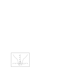
Figure 1: The harmonic oscillator without levels $\lambda_{2}$ and $\lambda_{3}$.

After the deletion of levels $\lambda_{3}$, $\lambda_{4}$, $\lambda_{6}$ and $\lambda_{7}$ we receive one very interesting potential which is shown on Figure 2. Finally, the Figure 3 represents the potential which is obtained through the elimination of the levels $\lambda_{4}-\lambda_{7}$.

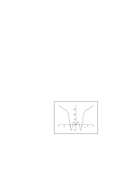
Figure 2: The harmonic oscillator without levels $\lambda_{3}$, $\lambda_{4}$, $\lambda_{6}$, $\lambda_{7}$.

The expressions for the potentials $v^{(n)}(y;\kappa)$, eigenfunctions (including the ground state) and tensions $\beta^{(n)}$ can be easily obtained via the (16) and (28). We omit them only for their extreme bulkiness.

The reason why these potentials have such Higgs-like form is evident. In fact, the spectrum of potential with two symmetric minimums necessarily contains the lacuna between two down levels and all other spectrum. Deleting the levels $\lambda_{3}$ and $\lambda_{4}$ we construct the spectrum with such lacuna so it is only natural that this procedure results in nothing else but Higgs-like potential. In a similar manner, elimination of the levels $\lambda_{4}-\lambda_{7}$ leads to the spectrum with lacuna between the three bottom levels and the other spectrum. As a result one get the potential with three minimums (Fig. 3). Note that all these potentials have the following asymptotic: $v^{(n)}(y;\kappa)\to 16b^{8}y^{2}/9$, when $y\to\pm\infty$.

Now lets return to potential (29). Using the exact forms of the $v^{(2)}$ and $\psi_{1}^{(2)}$ one can obtain the potential $V(\phi)$ in parametric form (i.e. $V=V(y)$ and $\phi=\phi(y)$). The plot of the function $d\phi(x)/dx$ for $y>0$ is represented on the Fig. 4. This expression is real for $\mid x\mid\geq x_{*}\sim 0.25735$ so if we identify the $\phi_{0}=x_{*}$ then the field $\phi(y)$ will be well determined all around the bulk.

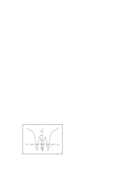
Figure 3: The harmonic oscillator without levels $\lambda_{4}-\lambda_{7}$.

Figure 4: The function $\phi^{\prime}(x)$.

IV.4 Dressing chains and the fourth Painlevé equation as the generalization of the odd superpotential

Another interesting generalization of the odd superpotential (i.e. the harmonic oscillator) can be obtained with the aid of the dressing chains of the DT, which chains were previously introduced in cepi . Let’s suppose, that we have defined the set of functions $f_{k}=\partial_{y}\log\psi_{k}^{(k-1)}$, where $\psi_{k}^{(n)}$ are $n$-times dressed solutions of the (8). Then these functions will also be solutions of the dressing chain:

$${\dot{f}}_{k}+{\dot{f}}_{k+1}=f_{k}^{2}-f_{k+1}^{2}+\alpha_{k}.$$ (30)

where $\alpha_{k}$ are constants, and they can be expressed via spectral parameters $\lambda_{k}$. Following cepi we’ll consider the periodic version $f_{k}=f_{k+N}$, $\alpha_{k}=\alpha_{k+N}$ with positive integer $N$ which will be further referred as period. The whole theories of dressing chains are totally different for the odd ($N=2n+1$) and even ($N=2n$) periods. The same is valid for the cases with $\alpha=0$ and $\alpha\neq 0$, where

$$\alpha=\sum_{k=1}^{N}\alpha_{k}.$$

If $\alpha\neq 0$ and $N=1$ we get the harmonic oscillator. In the case $N=3$ ($\alpha\neq 0$) we get the fourth Painlevé equation ($P_{{}_{IV}}$) for the function $P(y)=-f_{1}-y$:

$${\ddot{P}}=\frac{{\dot{P}}^{2}}{2P}+\frac{3}{2}P^{3}+4yP^{2}+2\left(y^{2}-a\right)P+\frac{b}{P},$$ (31)

where $\alpha=2$, $a=-\alpha_{1}-\alpha_{2}/2+1$, $b=-\alpha_{2}^{2}/2$. Thus the potential $v(y)={\dot{f}}_{1}+f_{1}^{2}$ can be expressed in term of the Painlevé-$IV$ transcendents and has the following behavior

$$v(y-y_{0})\sim\frac{\alpha^{2}y^{2}}{36}+My\cos\left(\frac{\alpha y^{2}}{\sqrt{3}}+\delta_{0}\right).$$ (32)

Using (32) one can conclude that this potential is indeed the generalization of the harmonic oscillator. In particular, this potential is growing quadratically.

We should also mention, that the spectrum of the $v(y)$ can be found explicitly cepi . Moreover, it can be shown that the ground state is at $\lambda_{1}=0$.

V The models with cosmological expansion

If we are going to study the models with cosmological expansion, we should expose the DT method to some kind of generalization. This requirement inevitably follows from the fact, that the substitution $A^{2}=\psi$ now results in nonlinear equation rather then in linear Schrödinger equation. However, seemingly being as difficult as it seems, this equation still can be reformulated in the way of linear spectral problem which does admit the Darboux transformation. In the next subsection we’ll consider the spacetimes which are compact in $y$. We’ll then introduce the simple orbifold $S_{1}/{\mathbb{Z}}_{2}$ and will show that, upon usage of DT, one can receive the solutions which result in exponentially small effective 4-D cosmological constant. In the last subsection we’ll briefly consider the new method which is valid for models both with and without cosmological expansion.

V.1 Noncompact spacetimes

If in (2) $H\neq 0$ then instead of (6) we have a much more complex system:

$$\begin{array}[]{c}\displaystyle{{\dot{u}}=-\frac{2{\dot{\phi}}^{2}}{3}-\frac{2H^{2}}{A}-\frac{2}{3}\sum_{b=1}^{N}\sigma_{b}\delta(y-y_{b})},\\ \displaystyle{u^{2}=\frac{{\dot{\phi}}^{2}}{3}-\frac{2}{3}V(\phi)+\frac{4H^{2}}{A},}\end{array}$$ (33)

written for the set of $N$ branes which are located at $y=y_{b}$.

The function $A^{2}$ solves the following nonlinear equation

$$\left(-\frac{d^{2}}{dy^{2}}-\frac{8}{3}V(\phi(y))+\frac{12H^{2}}{A}-\frac{4}{3}\sum_{b=1}^{N}\sigma_{b}\delta(y-y_{b})\right)A^{2}=0.$$ (34)

Therefore, we can formally introduce the spectral problem (the Schrödinger equation):

$${\ddot{\psi}(y;\lambda)}=\left(U(y)-\sum_{b=1}^{N}\beta_{b}\delta(y-y_{b})-\lambda\right)\psi(y;\lambda),$$ (35)

where

$${U(y)=-\frac{8}{3}V(\phi(y);\lambda)+\frac{12H^{2}}{\sqrt{\psi(y;\lambda)}}.}$$ (36)

We stress here, that $U(y)$ is not a function of the spectral parameter $\lambda$ whereas $V$ and $\psi$ are. With this induced, we are free to use the spectral theory for the equation (35). For any given $U(y)$ one can solve (35) to get $\psi$ and to find $V$ from (36). Of course, at the end of our solution we should, in order to find $A=\sqrt{\psi}$, receive $\psi$ of positive value, but this problem is also avoidable, as has been demonstrated in sections 3 and 4. Indeed, one can construct positive solution via the DT starting out from any simple solvable model - taking the RS model for example. There is, however, one interesting difference with the case of stationary brane: the ”kinetic term” appears to have the form

$$\frac{{\dot{\phi}}^{2}}{3}=\frac{1}{4}\left(\left(\frac{\dot{\psi}}{\psi}\right)^{2}-U+\lambda\right)-\frac{H^{2}}{\sqrt{\psi}},$$ (37)

therefore we can’t just use the ground state solution like we did in the case of stationary brane, or at $y\to\infty$ wave function $\psi\to 0$ and we will get ${\dot{\phi}}^{2}<0$. Obviously, this problem requires a more through examination. So, let’s again start out from an “RS potential” $U=\mu^{2}$, and consider the case $\lambda=0$. The solution will have the form (19). Using it as the prop function in (11), one gets the same metric $A^{(1)}_{\pm}$ from section 3, only with another potential. The main problem is now focused in the kinetic energy of the scalar field, having the form

$${({\dot{\phi}^{(1)}_{\pm}})^{2}=\frac{3\mu^{2}a_{{}_{\pm}}b_{{}_{\pm}}}{\left(a_{{}_{\pm}}e^{\mu y}+b_{{}_{\pm}}e^{-\mu y}\right)^{2}}-3H^{2}\sqrt{a_{{}_{\pm}}e^{\mu y}+b_{{}_{\pm}}e^{-\mu y}}.}$$

It is clear that for large enough $y$, one gets $\dot{\phi}^{2}<0$. On the other hand, if (see (21))

$$\left(\frac{H}{\mu}\right)^{2}<\frac{\sin^{2}2\alpha_{\pm}}{4r},$$

then on the brane and in its vicinity, there are no such troubles. Therefore the simplest way of avoiding the problem is just dealing with the finite volume, which is less then the minimum value of $y$, resulting in the negativity of the kinetic term.

If we nevertheless wish to deal with infinite volume, we had to be sure to use only those positive solutions $\psi(y)=\{\psi_{+}(y),\,\,{\rm at}\,\,y>0;\psi_{-}(y),\,\,{\rm at}\,\,y<0\}$ which are growing as $\mid y\mid\to\infty$. The construction of such solutions can be done in different manners. For example, one can take the solution of the Schrödinger equation with $\lambda=\lambda_{-1}<\lambda_{{}_{vac}}$. The more interesting opportunity lies in applying of so called B-potential (Bargmann potentials) $U(y)$ whose solutions of the Schrödinger equation all have the form: $\psi=F(y)\exp(\alpha y)$ where $F(y)$ is some polynomial Bargmann . To show them in work lets rewrite the equation (37) in the form

$$\frac{1}{3}{\dot{\phi}}^{2}_{{}_{\pm}}=-\frac{1}{2}{\dot{u}}_{{}_{\pm}}-\frac{H^{2}}{\sqrt{\psi_{{}_{\pm}}}},$$ (38)

where $u_{{}_{\pm}}={\dot{\psi}}_{{}_{\pm}}/(2\psi_{{}_{\pm}})$. The necessary criterion here is that ${\dot{u}}_{{}_{\pm}}<0$ for any given $y$. Let’s choose the $\psi_{{}_{\pm}}$ in typical ”Bargmann form”:

$$\psi_{{}_{\pm}}=\left(Ay^{2}\pm By+C\right){\rm e}^{\pm\alpha y},$$ (39)

where $\alpha$, $A$, $B$ and $C$ are positive constants, associated by the condition

$$2AC<B^{2}<4AC.$$ (40)

The jump condition (13), imposed to single brane at $y=0$ results in $\beta=-2(B+\alpha C)/C$ . The solution of the equation (33) appears to be

$$A_{{}_{\pm}}={\rm e}^{\pm\alpha y/2}\sqrt{Ay^{2}\pm By+C}.$$ (41)

where $A(y)=A_{{}_{+}}$ at $y>0$ and $A(y)=A_{{}_{-}}$ at $y<0$. The condition (40) guarantees that this solution will be nonsingular on brane as well as in bulk (since $A(y)\neq 0$ for any values of $y$) and also that ${\dot{u}}_{{}_{+}}<0$ for $y>0$ and ${\dot{u}}_{{}_{-}}<0$ for $y<0$. Finally, choosing

$$H^{2}<\frac{B^{2}-2AC}{4C\sqrt{C}},$$

and using (41) and (38) one get

$$\frac{{\dot{\phi}}^{2}_{{}_{\pm}}}{3}=\frac{2A^{2}y^{2}\pm 2ABy+B^{2}-2AC}{4(Ay^{2}\pm By+C)^{2}}-\frac{H^{2}{\rm e}^{\mp\alpha y/2}}{\sqrt{Ay^{2}\pm By+C}},$$

where $\phi(y)=\phi_{{}_{+}}$ at $y>0$ and $\phi(y)=\phi_{{}_{-}}$ at $y<0$. Now we can see, that it is always possible to find large enough values of $\alpha$ that will greatly decrease the second member of equation with regard to the first, thus leaving the whole equation positive for both $y>0$ and $y<0$.

V.2 Orbifold model

In previous sections, our efforts were wholly concentrated on spacetimes that are noncompact in $y$. Now we’ll consider the compactified case. As we shall see, the DT in this case allows to obtain the solutions, resulting in exponentially small 4-D effective cosmological constant.

Let’s choose the potential in (35) as $U=\mu^{2}\sin^{2}\theta$. We’ll start with the two solution of this equation:

$$\psi_{{}_{1}}=\cosh(\mu\sin\theta y),\qquad\psi_{{}_{2\pm}}=\sinh(\mu y\pm b),$$

where $b=$const. The function $\psi_{{}_{1}}$ is the solution of the (35) with $\lambda_{1}=0$ whereas $\psi_{{}_{2\pm}}$ with $\lambda_{2}=-\mu^{2}\cos^{2}\theta$. Using $\psi_{{}_{1}}$ as the prop function we can dress $\psi_{{}_{2\pm}}$ with the help of the DT (11). The result will be

$$\psi^{(1)}_{{}_{2\pm}}=\cosh(\mu y\pm b)-\sin\theta\tanh(\mu\sin\theta y)\sinh(\mu y\pm b).$$ (42)

where we should choose the sign ”$+$” for $y>0$ and sign ”$-$” for $y<0$. One can show that $\psi^{(1)}_{{}_{2\pm}}>0$ for all $y$. In this case the dressed potential $U^{(1)}$ will have the single bound state with $\lambda=\lambda_{1}$ and eigenfunction $1/\psi_{{}_{1}}$.

Now we can compactify the $y$ direction as an ${\mathbb{Z}}_{2}$ orbifold, with two branes sitting at each of the two fixed points ($y=0$ and $y=L$). The new aspect here is that $S_{1}/{\mathbb{Z}}_{2}$ orbifold model permits only one bulk space. Due to the symmetry of the model, we only have to consider the jump conditions at $y=0$ and $y=L$. The direct calculations result in tension $\sigma_{0}=-3\mu\tanh b\cos^{2}\theta/2$ for the brane which is located at $y=0$ (we’ll choose it as the visible brane) and

$$\sigma_{{}_{L}}=-\frac{3\mu}{2}\frac{\sinh(\mu L+b)(\cosh^{2}(\mu\sin\theta L)-\sin^{2}\theta)-\sin\theta\sinh(\mu\sin\theta L)\cosh(\mu\sin\theta L)\cosh(\mu L+b)}{\cosh(\mu\sin\theta L)\left(\sin\theta\sinh(\mu\sin\theta L)\sinh(\mu L+b)-\cosh(\mu\sin\theta L)\cosh(\mu L+b)\right)},$$

as a tensions on $y=L$ branes. These expressions can be greatly simplified by the choice $b=-\mu L$:

$$\begin{array}[]{cc}\displaystyle{\sigma_{0}=\frac{3\mu}{2}\tanh(\mu L)\cos^{2}\theta,}\\ \\ \displaystyle{\sigma_{{}_{L}}=-\frac{3\mu}{2}\tanh(\mu\sin\theta L)\sin\theta.}\end{array}$$

Since the expansion rate on the visible brane is $H(0)=H/\sqrt{A(0)}=H/\left(\psi^{(1)}_{{}_{2\pm}}(0)\right)^{1/4}$ then

$$H(0)=\frac{H}{{}^{4}\sqrt{\cosh(\mu L)}}.$$

Therefore, for large values of $\mu L$ the effective 4-D cosmological constant $\Lambda_{eff}$ on the visible brane is

$$\Lambda_{eff}\sim H^{2}(0)=\frac{H^{2}}{\sqrt{\cosh(\mu L)}}\sim H^{2}{\rm e}^{-\mu L/2}.$$ (43)

This means, that 4-dimensional cosmological constant, as seen by observers from the visible brane, becomes exponentially small while the $L$ grows large, therefore, automatically solving the cosmological constant problem right in the framework of the the brane worlds models (this idea was first suggested in article of S.-H.H. Tye and I. Wasserman TW ).

All we need now is to make sure, that ${\dot{\phi}}^{2}_{{}_{+}}>0$ at $0<y<L$ (since we have the single bulk between two branes then it is enough to consider the case $0<y<L$ solely). Let’s choose $\theta\sim\pi/2$. In this case $\lambda_{2}\sim\lambda_{1}=0$. We stress, however, that $\theta\neq\pi/2$ exactly so $\lambda_{2}=-\mu^{2}\alpha^{2}$ where $\alpha=\pi/2-\theta\ll 1$. To obtain ${\dot{\phi}}^{2}_{{}_{+}}(0)>0$ it is necessary that $\cosh(\mu L)>16H^{4}/\mu^{4}$ whereas ${\dot{\phi}}^{2}_{{}_{+}}(L)>0$ if $\cosh(\mu L)<\mu/(2H)$. The combination of these conditions is:

$$\left(\frac{2H}{\mu}\right)^{4}<\cosh(\mu L)<\frac{\mu}{2H},$$

which is possible if $\mu>2H$. In fact, it is better to imply an enhanced condition $\mu\gg 2H$, because large values of $\mu$ allows to avoid the conclusion that $\sigma_{0}=3\mu\alpha^{2}/2\sim 0$. Since $\mu$ is not bounded from above, we draw the wanted conclusion, that our model indeed permits positive ${\dot{\phi}}^{2}_{{}_{+}}$ at $0<y<L$.

Nota Bene 3. Of course, the described theory could not generally protect some finite number of regions (at $0<y<L$) from special situations when ${\dot{\phi}}^{2}_{{}_{+}}(y)<0$ (if the value of $\mu$ is not sufficiently large, for example). In this case, however, one can use the method which was supposed in Yurov , viz. these regions can be cut out, with their boundaries being sewn together in such a way that neither the warp factor (along with its first two derivatives) nor Ricci scalar will experience a jump. This unexpected fortune raises from the fact that matching is done at an inflection point of $\log A$ (more correctly, this is approximately true if $\psi$ is sufficiently large to neglect the term $H/\sqrt{\psi}$ in either one of equations (37) and (38)).

V.3 Green function method

This is another way to construct solution for the models with cosmological expansion. First of all, we can directly transform the system (33) into the linear equation rather than use substitution $\psi=A^{2}$. Indeed, introducing the potential

$$\textrm{U}\equiv-\frac{2}{3}\left(\frac{{\dot{\phi}}^{2}}{2}+V(\phi)\right),$$

we get (for the case of single brane located at $t=0$)

$$-{\ddot{A}}+\left(\textrm{U}-\frac{2}{3}\sigma_{0}\delta(y)\right)A=-2H^{2}.$$ (44)

Solving linear nonhomogeneous equation (44) for given U we can find $\phi(y)$ and $V(\phi)$ via the system

$$\begin{array}[]{cc}\displaystyle{{\dot{\phi}}^{2}=-\frac{3}{2}\left(\textrm{U}-\left(\frac{\dot{A}}{A}\right)^{2}\right)-\frac{6H^{2}}{A}},\\ \displaystyle{V=-\frac{3}{4}\left(\textrm{U}+\left(\frac{\dot{A}}{A}\right)^{2}\right)+\frac{3H^{2}}{A}}.\end{array}$$

Now, instead of the (44) let’s consider the nonhomogeneous spectral problem

$$-{\ddot{\psi}}(y;\lambda)+\left(\textrm{U}(y)-\lambda-\frac{2}{3}\sigma_{0}\delta(y)\right)\psi(y;\lambda)=-2H^{2}.$$

which can be written as

$${\bf L}(y;\lambda)\psi(y;\lambda)=-2H^{2},$$ (45)

with ${\bf L}(y;\lambda)=d^{2}/dy^{2}+U(y)-\lambda-2\sigma_{0}\delta(y)/3$.

To solve (45) we introduce the homogeneous linear equation

$${\bf L}(y;\lambda)\psi_{0}(y;\lambda)=0,$$ (46)

and the Green function $G(y,z;\lambda)$:

$${\bf L}(y;\lambda)G(y,z;\lambda)=\delta(y-z).$$

By solving these equation for given $U(y)$ and $\lambda$ we can construct the solution of (45) as

$$\psi(y;\lambda)=\psi_{0}(y;\lambda)-2H^{2}\int dz\,G(y,z;\lambda).$$

If $\psi(y;\lambda)$ will be positive then we will be able to define $A=\sqrt{\psi}$ just like before. But first we have to determine those conditions which make such positive solutions possible. This is still the open question which will be considered in the next publications. We should only note, that Green function can be constructed via solutions of the (46). If initial potential $\textrm{U}(y)$ is exactly solvable one, then the same is true for N-times Darboux dressed potential $\textrm{U}^{(N)}$. Thus, if we know the Green function $G(y,z;\lambda)$ of the initial equation then we know the Green function $G^{(N)}(y,z;\lambda)$ for equation with the dressed potential. In other words, the DT is appliable here, at least formally.

VI Conclusion

This approach can be easily generalized to the case of $K$-branes. For this we should replace the term $\beta\delta(y)$ in (8) by

$$\sum_{b}\beta_{b}\delta(y-y_{b}),$$

and also replace the two jump conditions (13) by $2K$ jump conditions at $y=y_{b}$. This is nothing more than technical matter, that’s why we omit the details.

Another one kettle of fish is that even in case of general position, where we cannot reconstruct the form of the potential $V(\phi)$ as a function of $\phi$, all these solutions will have the RS asymptotics (of course, if constructed precisely according to section 3). The DT gives a link between the solvable problems, and probably most (if not all) of the exactly solvable potentials, from the potential of the harmonic oscillator to the finite-gap potentials cepi , can all be obtained via these transformations. The physical sense of these potentials in the brane world is not clear. But our main purpose in this work was to merely demonstrate and advertise the DT as being the very powerful tool for manufacturing the exactly solvable potentials in the 5-D gravity with the bulk scalar field. It has been demonstrated that this method can be useful both in models with and without the cosmological expansion, although in the first case the situation is more complex and deserves the further studying. Notably, there is one imperfection of this method: the DT would work for the 5-D gravity only. If $D>5$ then the warp factor is a multi-variable function. Unfortunately, there is no cogent and effective general DT theory in several dimensions D-Moutard . But, nevertheless, for $D=5$ the DT is by far seems to be the best way to construct the nonsingular exact solutions.

References

1. E.E. Flanagan, S.-H.H. Tye and I. Wasserman,   Phys. Lett. B 522, (2001), 155-165, [hep-th/0110070 v2].
2. If the observed cosmological accelerated expansion is generated by the nonzero cosmological constant, the 4-D metric in (2) can, in fact, describe our universe - of course, in case of future distant enough. See S. Perlmutter et al., Astrophys. J. 517, 565 (1999) [astro-ph/9812133]; A. G. Riess et al., Astron. J. 116, 1009 (1998) [astro-ph/9805201]; P. M. Garnavich et al., Astrophys. J. 509, 74 (1998) [astro-ph/9806396].
3. L. Randall and R. Sundrum,   Phys. Rev. Lett. 83, 3370 (1999), [hep-th/9906064].
4. S.-H.H. Tye and I. Wasserman,  Phys. Rev. Lett. 86 1682 (2001) [hep-th/0006068].
5. O. DeWolf, D.Z. Freedman, S.S. Gubser and A. Karch,  Phys. Rev. D62, 046008 (2000), hep-th/9909134.
6. Z. Kakushadze, Nucl. Phys. B 589, 75 (2000) [hep-th/0005217].
7. V.B. Matveev and M.A. Salle.  Darboux Transformation and Solitons. Berlin–Heidelberg: Springer Verlag, 1991.
8. A.A. Andrianov, N.V. Borisov and M.V. Ioffe, Phys.Lett.A(105) 19 (1984); A.A. Andrianov, N.V. Borisov M.I. Eides and M.V. Ioffe, Phys.Lett.A(109) 143 (1984).
9. W. Israel, Nuovo Cimento B 44 (S10) 1 (1966); V.A. Berezin, V.A. Kuzmin and I.I. Tkachev, Phys. Rev. D36, 2919 (1987).
10. R.R. Caldwell, M. Kamionkowski and N.N. Weinberg, [astro-ph/0302506].
11. R.R. Caldwell, Phys. Lett. B 545, 23-29 (2002) [astro-ph/9908168].
12. S.M. Carroll, M. Hoffman and M. Trodden, [astro-ph/0301273].
13. H.-P. Nilles, Phys. Rep. 110, 1-162 (1984).
14. M.D. Pollock, Phys. Lett. B 215, 635-641 (1988).
15. V. Sahni and Y. Shtanov, [astro-ph/0202346].
16. J.G. Darboux   Compt.Rend., 94 p.1343 (1882).
17. B.P. Berezovoy, A.I. Pashnev, Theor. and Math. Phys., v.70, N1, 146 (1987).
18. V.A. Rubakov, Uspehi Fiz. Nauk 171, 913 (2001).
19. M.M. Crum   Quart. J. Math. Ser. Oxford 2, 6 p. 121 (1955).
20. Thereby, defining the integration’s constants $C_{1}=1$ and $C_{2}=0$, which is distinct for a ground state.
21. L. Infeld and T.E. Hull,   Rev.Mod.Phys. V. 23 p. 21 (1951).
22. V.E. Adler, Theor. and Math. Phys., v.101, N3, 323 (1994).
23. As a matter of fact, in the case of Bargmann potentials the solutions of the Schrödinger equation have the form $P(k)\exp(iky)$, where $P(k)$ is some polynomial. We use some generalization of B-potentials. See V. Bargmann, Rev. Mod. Phys. 21, 488-493 (1949).
24. A.V. Yurov, S.D. Vereshchagin, Theoretical and Mathematical Physics, 139 (3): 787-800 (2004); A.V. Yurov, [astro-ph/0305019].
25. A.P. Veselov and A.B. Shabat,  Funkts. Anal. Prilozhen., Vpl. 27, No. 2, p. 1 (1993).
26. A. Gorizales-Lopes and N. Kamran, J.Geom.Phys.26202-226 (1998) [hep-th/9612100].