The finite-temperature chiral transition in QCD with adjoint fermions

Abstract:

We study the nature of the finite-temperature chiral transition in QCD with $N_{f}$ light quarks in the adjoint representation (aQCD). Renormalization-group arguments show that the transition can be continuous if a stable fixed point exists in the renormalization-group flow of the corresponding three-dimensional $\Phi^{4}$ theory with a complex $2N_{f}\times 2N_{f}$ symmetric matrix field and symmetry-breaking pattern ${\rm SU}(2N_{f})\rightarrow{\rm SO}(2N_{f})$. This issue is investigated by exploiting two three-dimensional perturbative approaches, the massless minimal-subtraction scheme without $\epsilon$ expansion and a massive scheme in which correlation functions are renormalized at zero momentum. We compute the renormalization-group functions in the two schemes to five and six loops respectively, and determine their large-order behavior.

The analyses of the series show the presence of a stable three-dimensional fixed point characterized by the symmetry-breaking pattern ${\rm SU}(4)\rightarrow{\rm SO}(4)$. This fixed point does not appear in an $\epsilon$-expansion analysis and therefore does not exist close to four dimensions. The finite-temperature chiral transition in two-flavor aQCD can therefore be continuous; in this case its critical behavior is determined by this new SU(4)/SO(4) universality class. One-flavor aQCD may show a more complex phase diagram with two phase transitions. One of them, if continuous, should belong to the O(3) vector universality class.

1 Introduction

The thermodynamics of Quantum Chromodynamics (QCD) is characterized by a transition from a low-temperature hadronic phase, in which chiral symmetry is broken, to a high-temperature phase with deconfined quarks and gluons (quark-gluon plasma), in which chiral symmetry is restored. See, e.g., Refs [1, 2, 3, 4] for recent reviews. Although deconfinement and chiral symmetry restoration are apparently related to different nonperturbative mechanisms, they seem to be somehow coupled in QCD. Indeed, lattice computations show that the Polyakov loop has a sharp increase around the critical temperature where the chiral condensate vanishes [2]. However, the interplay between the two effects is not clear yet.

Insight into this question may be gained by investigating QCD-related models, such as ${\rm SU}(N_{c})$ gauge theories with $N_{f}$ Dirac fermions in the adjoint representation (aQCD). In aQCD with $N_{f}$ massless flavors the chiral symmetry group is ${\rm SU}(2N_{f})$, which is expected to be spontaneusly broken to ${\rm SO}(2N_{f})$ at low temperature [5, 6, 7, 8, 9], due to the presence of a nonzero quark condensate. In addition, unlike QCD with fermions in the fundamental representation, aQCD is also invariant under global ${\mathbb{Z}}_{N_{c}}$ transformations corresponding to the center of the SU($N_{c}$) gauge group, as is the case in pure ${\rm SU}(N_{c})$ gauge theories. This symmetry breaks down in the high-temperature deconfined phase. Therefore, in aQCD one expects two finite-temperature transitions: a deconfinement transition at $T_{d}$ associated with the breaking of the ${\mathbb{Z}}_{N_{c}}$ symmetry, and a chiral transition at $T_{c}$ characterized by the symmetry-breaking pattern ${\rm SU}(2N_{f})\rightarrow{\rm SO}(2N_{f})$. Of course, it is also possible to have only one transition if the corresponding critical temperatures coincide. We should mention that this issue is interesting only for the values of $N_{f}$ for which aQCD is asymptotically free. Since the first coefficient $b_{0}$ of the $\beta$ function $\beta(g)=-b_{0}g^{4}+O(g^{6})$ of SU($N_{c}$) gauge theories with $N_{f}$ adjoint Dirac fermions is $b_{0}=(11-4N_{f})N_{c}/(24\pi^{2})$, aQCD is asymptotically free only for $N_{f}<11/4$, i.e., for $N_{f}=1$ and $N_{f}=2$.

Monte Carlo simulations of ${\rm SU}(2)$ [10, 11] and SU(3) [12] gauge theories with two adjoint fermions show that the deconfinement and chiral transitions are well separated with $T_{d}<T_{c}$. In the case of three-color aQCD, the Monte Carlo simulations reported in Ref. [12] show actually that the ratio $T_{c}/T_{d}$ is rather large, $T_{c}/T_{d}\simeq 8$, suggesting a rather weak interplay between the corresponding underlying mechanisms. They provide a rather clear evidence that the deconfinement transition associated with the center symmetry ${\mathbb{Z}}_{3}$ is of first order. Moreover, the available data at the chiral transition are apparently consistent with a continuous transition. However, they should be considered as rather preliminary and not conclusive, since a careful analysis of finite-size effects and of the approach to the continuum limit has not been done yet. The phase diagram of two-color aQCD in the temperature–chemical-potential plane has been recently discussed in Ref. [13].

In this paper we investigate the nature of the finite-temperature chiral transition in aQCD, i.e. in four-dimensional ${\rm SU}(N_{c})$ gauge theories with adjoint fermions, using renormalization-group (RG) arguments. Our study parallels the ones reported in Refs. [14, 15], in which the nature of the finite-temperature transition in QCD with fermions in the fundamental representation was investigated. We consider effective three-dimensional Landau-Ginzburg-Wilson (LGW) $\Phi^{4}$ theories for the low-momentum critical modes associated with the bilinear quark condensate, which are described by a symmetric complex $2N_{f}\times 2N_{f}$ matrix field, and look for stable fixed points (FPs) that may be associated with the symmetry-breaking pattern relevant for aQCD: ${\rm SU}(2N_{f})\rightarrow{\rm SO}(2N_{f})$ [if the axial U(1) symmetry is effectively restored at $T_{c}$ the symmetry-breaking pattern would be ${\rm U}(2N_{f})\rightarrow{\rm O}(2N_{f})$]. If such a stable FP does not exist the transition is of first order; otherwise, the transition may be continuous or of first order, depending whether the system is or is not in the attraction domain of the stable FP. We study the RG flow of the LGW theories in two field-theoretical (FT) perturbative approaches: the minimal-subtraction scheme without $\epsilon$ expansion (in the following we will indicate it as $3d$-$\overline{\rm MS}$ scheme) [16] and a massive zero-momentum (MZM) renormalization scheme [17]. In the $3d$-$\overline{\rm MS}$ scheme one considers the massless (critical) theory in dimensional regularization [18], determines the RG functions from the divergences appearing in the perturbative expansion of the correlation functions, and finally sets $\epsilon\equiv 4-d=1$ without expanding in powers of $\epsilon$ (this scheme therefore differs from the standard $\epsilon$ expansion [19]). In the MZM scheme one considers instead the three-dimensional massive theory, corresponding to the disordered (high-temperature) phase, and determines the renormalization constants from zero-momentum correlation functions. We compute the $\beta$ functions perturbatively to five loops in the $3d$-$\overline{\rm MS}$ scheme and to six loops in the MZM scheme. They are resummed by using a conformal-mapping method [20, 21] taking into account their large-order behavior, determined by means of the standard semiclassical analysis of instanton solutions. Comparison of the results of these two perturbative schemes provides a nontrivial check of the reliability of our conclusions.

We briefly summarize our main results. In both $3d$-$\overline{\rm MS}$ and MZM schemes the three-dimensional SU(4) LGW $\Phi^{4}$ theory relevant for aQCD with two Dirac flavors shows a stable FP, that corresponds to a new three-dimensional universality class characterized by the symmetry-breaking pattern ${\rm SU}(4)\rightarrow{\rm SO}(4)$. The corresponding critical exponents are $\eta\approx 0.2$ and $\nu\approx 1.1$. Note that this FP does not appear in an $\epsilon$-expansion analysis ($\epsilon\equiv 4-d$) and therefore does not exist close to four dimensions. It is found only in genuinely three-dimensional analyses. This FT result implies that the finite-temperature chiral transition in two-flavor aQCD may be continuous. In this case, it belongs to the above-mentioned three-dimensional SU(4)/SO(4) universality class. However, this does not exclude a first-order transition for systems that are outside the attraction domain of the stable FP. Note that, although SU(4) is locally isomorphic to SO(6), this universality class is definitely different from the vector O(6) one, whose symmetry-breaking pattern is SO(6)$\rightarrow$SO(5). No stable FP is found for the U(4) LGW $\Phi^{4}$ theory which should be relevant in the case the axial U(1) symmetry is effectively restored at $T_{c}$; in this case, the transition would be of first order. For $N_{f}=1$ the phase diagram may be more complex because the phase diagram of the corresponding SU(2)-symmetric effective theory has several transition lines joining at a multicritical point. In the parameter region relevant for aQCD, the possible phase diagrams have one or two phase transitions. One of them would be associated with the symmetry-breaking pattern ${\rm SU}(2)/{\mathbb{Z}}_{2}\cong{\rm SO}(3)\rightarrow{\rm SO}(2)$. Therefore, if continuous, the transition would belong to the standard O(3) (Heisenberg) universality class. The second transition, which could be absent in aQCD, would correspond to the symmetry-breaking pattern ${\mathbb{Z}}_{2}\otimes{\rm SO}(2)\to{\rm SO}(2)$, and, if continuous, would correspond to the Ising universality class. Note that the symmetry breaking ${\rm SU}(2)\to{\rm SO}(2)$ occurs in this case through two different phase transitions.

The predicted critical behavior for two-flavor aQCD should be compared with that of two-flavor QCD with quarks in the fundamental representation. Also in this last case the finite-temperature chiral transition may be continuous, although it would belong to a different universality class, the vector O(4) universality class. Monte Carlo simulations of lattice QCD [22, 23, 2, 4] seem to be consistent with a continuous transition in the O(4) universality class, although they are not yet sufficiently precise to be conclusive.

The paper is organized as follows. In Sec. 2 we derive the LGW $\Phi^{4}$ theory relevant for the finite-temperature chiral transition in aQCD, using universality and RG arguments. In Sec. 3 we investigate the RG flow of the LGW theory with U($N$) symmetry, which would be relevant for aQCD if the U(1) anomaly were effectively suppressed at $T_{c}$. We report our perturbative calculations in the $3d$-$\overline{\rm MS}$ and MZM renormalization schemes and their analyses. In Sec. 4 we consider a more general LGW theory in which the U($N$) symmetry is explicitly broken to SU($N$). We discuss the one-flavor case and present a perturbative analysis for $N=4$, which is relevant for two-flavor aQCD. The appendix contains an analysis of the vacuum structure of the LGW $\phi^{4}$ theories relevant for aQCD.

2 The effective Landau-Ginzburg-Wilson model at the chiral transition

In the vanishing quark-mass limit, the fermionic part of the QCD Lagrangian with $N_{f}$ adjoint Dirac fermions is given by ${\cal L}=\sum_{f}\bar{\psi}_{f}\gamma_{\mu}D_{\mu}\psi_{f}$, where $D_{\mu}^{ab}=\partial_{\mu}\delta^{ab}+iA_{\mu}^{c}f_{c}^{ab}$ and $f_{c}^{ab}$ are the generators of the adjoint representation, i.e. the structure constants. Using the antisymmetry of the structure costants, one may rewrite the Lagrangian in terms of two-component Weyl spinors as ${\cal L}=i\sum_{i=1}^{2N_{f}}w_{i}^{\dagger}\sigma_{\mu}D_{\mu}w_{i}$, where $\sigma_{\mu}\equiv({\rm Id},\vec{\sigma})$, ${\rm Id}$ is the identity matrix, and $\sigma_{i}$ are the Pauli matrices; see, e.g., Refs. [7, 8, 9]. The actual symmetry is ${\rm U}(2N_{f})\cong{\rm U}(1)_{A}\otimes[{\rm SU}(2N_{f})/{\mathbb{Z}}_{2N_{f}}]$, which is larger than the symmetry ${\rm U}(N_{f})_{R}\otimes{\rm U}(N_{f})_{L}$ of QCD with fermions in the fundamental representation. The U(1)_A subgroup is anomalous at the quantum level and thus the symmetry reduces to ${\rm SU}(2N_{f})$.

At $T=0$ the symmetry is expected to be spontaneously broken due to a nonzero quark condensate $\langle\bar{\psi}\psi\rangle$. As a consequence of the Pauli principle, the quark bilinear condensate must belong to the symmetric second-rank tensor representation of ${\rm SU}(2N_{f})$, which has dimension $2N_{f}^{2}+N_{f}$. Condensation along one of its directions gives rise to the symmetry breaking

$${\rm SU}(2N_{f})\rightarrow{\rm SO}(2N_{f})$$ (1)

and to $2N_{f}^{2}+N_{f}-1$ Goldstone modes. See, e.g., Refs. [7, 8, 9] for more details. With increasing the temperature, a phase transition characterized by the restoring of the chiral symmetry is expected at a given $T_{c}$; above $T_{c}$ the quark condensate vanishes. Therefore, the finite-temperature phase transition is characterized by the symmetry-breaking pattern (1) and a complex symmetric $2N_{f}\times 2N_{f}$ matrix order parameter $\Phi_{ij}$. In the case the U(1) symmetry is effectively restored at $T_{c}$, the relevant symmetry-breaking pattern would be

$${\rm U}(2N_{f})\rightarrow{\rm O}(2N_{f}).$$ (2)

This possibility is however rather unlikely. Indeed, instanton calculations in the high-temperature phase [24] suggest that the axial U(1) symmetry is not restored at $T_{c}$, in analogy with what happens in lattice QCD with fermions in the fundamental representation [25], and as also suggested by the finite-temperature behavior of the topological susceptibility in the pure SU($N_{c}$) gauge theories, see, e.g., Ref. [26].

In order to investigate the nature of the finite-temperature transition in aQCD with $N_{f}$ light flavors, we follow the reasoning already applied in Refs. [14, 15] to the study of the finite-temperature transition in QCD with light fermions in the fundamental representation.

• Let us first assume that the phase transition at $T_{c}$ is continuous (second order) for vanishing quark masses. In this case the critical behavior should be described by an effective three-dimensional (3-$d$) theory. Indeed, the length scale of the critical modes diverges approaching $T_{c}$, becoming eventually much larger than $1/T_{c}$, which is the size of the euclidean “temporal” dimension at $T_{c}$. Therefore, the asymptotic critical behavior must be associated with a 3-$d$ universality class characterized by a complex symmetric $2N_{f}\times 2N_{f}$ matrix order parameter $\Phi_{ij}$ and by the symmetry-breaking pattern (1) [or (2) if the U(1) symmetry is effectively restored at $T_{c}$].

• According to RG theory, the existence of such universality classes can be investigated by considering the most general LGW $\Phi^{4}$ theory for a complex symmetric $N\times N$ matrix field $\Phi_{ij}$ with $N=2N_{f}$ and the desired symmetry and symmetry-breaking pattern. The most general ${\rm U}(N)$-symmetric LGW Lagrangian containing up to quartic terms in the potential is

  $${\cal L}_{U(N)}={\rm Tr}\,(\partial_{\mu}\Phi^{\dagger})(\partial_{\mu}\Phi)+r{\rm Tr}\,\Phi^{\dagger}\Phi+{u_{0}\over 4}\left({\rm Tr}\,\Phi^{\dagger}\Phi\right)^{2}+{v_{0}\over 4}{\rm Tr}\left(\Phi^{\dagger}\Phi\right)^{2}.$$ (3)

  Stability requires $u_{0}+v_{0}>0$ and $Nu_{0}+v_{0}>0$. The symmetry group of this Lagrangian is U($N$). First, it is invariant under the transformations $\Phi\rightarrow U\Phi U^{T}$, where $U$ is a unitary ${\rm U}(N)$ matrix, i.e., under the group U($N$)/${\mathbb{Z}}_{2}$ (the quotient ${\mathbb{Z}}_{2}$ is due to the fact that matrices $\pm U$ give rise to the same transformation). Second, it is invariant under $\Phi\to\Phi^{\dagger}$. The symmetry group is therefore ${\mathbb{Z}}_{2}\otimes$U($N$)/${\mathbb{Z}}_{2}\cong{\rm U(}N)$. For $v_{0}>0$, Lagrangian (3) shows the expected vacuum structure and symmetry-breaking pattern, see appendix. In the low-temperature phase the potential is minimized by taking

  $$\phi_{\rm min}\propto\left(\begin{array}[]{cc}0&{\rm Id}\\ {\rm Id}&0\end{array}\right),$$ (4)

  where ${\rm Id}$ is the $N/2$-dimensional identity matrix. Note that $\Phi_{\rm min}$ is invariant under vector ${\rm U}(N_{f})_{V}$ transformations, in agreement with the Vafa-Witten theorem [6]. The symmetry of the vacuum is O($N$) and thus the symmetry breaking pattern is ${\rm U}(N)\to{\rm O(}N)$.

  The axial anomaly reduces the symmetry to ${\rm SU}(N)$ and thus new terms must be added. The most relevant one is proportional to $\left({\rm det}\,\Phi^{\dagger}+{\rm det}\,\Phi\right)$, which is a polynomial of order $N$ in the field $\Phi$. For $N>4$ such a term is irrelevant at the transition. Instead, for $N=2$ and $N=4$, the determinant must be added to Lagrangian (3), obtaining

  $${\cal L}_{SU(N)}={\cal L}_{U(N)}+w_{0}\left({\rm det}\,\Phi^{\dagger}+{\rm det}\,\Phi\right).$$ (5)

  For $N=2$ additional terms depending on the determinant of $\Phi$ should be added, in order to include all terms with at most four fields compatible with the symmetry. They will be discussed in Sec. 4.1. The symmetry of Lagrangian (5) is ${\mathbb{Z}}_{2}\otimes{\rm SU}(N)$. Indeed, it is invariant under transformations $\Phi\to U\Phi U^{T}$, with $U$ unitary and ${\rm det}\,U=\pm 1$. Taking into account that $U$ and $-U$ correspond to the same transformation, the invariance group is SU($N$). Moreover, the model is invariant under the ${\mathbb{Z}}_{2}$ transformations $\Phi\to\Phi^{\dagger}$. For $v_{0}>-3|w_{0}|/2$, the vacuum structure is identical to that discussed for the U($N$) theory, satisfying the Vafa-Witten theorem [6]. The corresponding symmetry-breaking pattern is ${\mathbb{Z}}_{2}\otimes{\rm SU}(N)\to{\mathbb{Z}}_{2}\otimes{\rm SO}(N)$. Note that the symmetry group contains an additional ${\mathbb{Z}}_{2}$ with respect to Eq. (1). This additional invariance, related to the transformation $\Phi\to\Phi^{\dagger}$, is a consequence of the hermiticity (reality) of the effective Lagrangian and corresponds to the discrete parity symmetry of the aQCD Lagrangian. This additional ${\mathbb{Z}}_{2}$ is not broken at the transition, so that the relevant symmetry-breaking pattern is indeed ${\rm SU}(N)\to{\rm SO}(N)$, as discussed before. It must be noted that, if a $\theta$ term is added to the aQCD Lagrangian, this additional symmetry is not present and the effective Lagrangian is no longer hermitian.

• The critical behavior at a continuous transition is described by the stable FP of the theory, which determines the universality class. The absence of a stable FP indicates that the phase transition is not continuous. Therefore, a necessary condition of consistency with the initial hypothesis that the transition is continuous, cf. (i), is the existence of stable FPs in the theories described by Lagrangians (3) and (5). If a FP exists, the transition may be either continuous, belonging to the universality class associated with the stable FP, or of first-order, if the system is not in the attraction domain of the FP.

The effective theories (3) and (5) are defined for any $N$. However, for aQCD they are relevant only for $N$ even and $N\leq 4$, i.e., for $N=2$ and $N=4$. Indeed, aQCD is asymptotically free only for $N_{f}<11/4$, i.e., for $N<11/2$.

3 Renormalization-group flow of the U($N$) LGW theory

3.1 Perturbative expansions

In order to investigate the RG flow of Lagrangians (3) and (5), we employ two different perturbative approaches: the MZM renormalization scheme [17] and the $3d$-$\overline{\rm MS}$ scheme [16]; see Refs. [21, 27] for recent reviews. In the first case, one considers the three-dimensional massive theory corresponding to the disordered phase, and expresses the zero-momentum renormalization constants in terms of zero-momentum renormalized quartic couplings. In the second case, one considers the massless (critical) theory in dimensional regularization within the minimal-subtraction scheme [18]. RG functions are obtained in terms of the renormalized couplings and of $\epsilon\equiv 4-d$. Subsequently $\epsilon$ is set to its physical value $\epsilon=1$, providing a three-dimensional scheme in which the 3-$d$ RG functions are expanded in powers of the $\overline{\rm MS}$ renormalized quartic couplings. This scheme differs from the standard $\epsilon$ expansion [19] in which one expands the RG functions in powers of $\epsilon$.

In order to renormalize the ${\rm U}(N)$-invariant theory (3) in the $\overline{\rm MS}$ scheme, one sets

$$\Phi = [Z_{\phi}(u,v)]^{1/2}\Phi_{R},$$ (6)

$$u_{0} = A_{d}\mu^{\epsilon}Z_{u}(u,v),$$

$$v_{0} = A_{d}\mu^{\epsilon}Z_{v}(u,v),$$

where $u$ and $v$ are the $\overline{\rm MS}$ renormalized quartic couplings. The renormalization constants $Z_{\phi}$, $Z_{u}$, and $Z_{v}$ are normalized so that $Z_{\phi}(u,v)\approx 1$, $Z_{u}(u,v)\approx u$, and $Z_{v}(u,v)\approx v$ at tree level. Here $A_{d}$ is a $d$-dependent constant given by $A_{d}\equiv 2^{d-1}\pi^{d/2}\Gamma(d/2)$. Moreover, one defines a mass renormalization constant $Z_{t}(u,v)$ by requiring $Z_{t}\Gamma^{(1,2)}$ to be finite when expressed in terms of $u$ and $v$. Here $\Gamma^{(1,2)}$ is the one-particle irreducible two-point function with one insertion of ${\rm Tr}\,\Phi^{\dagger}\Phi$. The $\beta$ functions are computed from

$$\beta_{u}(u,v)=\mu\left.{\partial u\over\partial\mu}\right|_{u_{0},v_{0}},\qquad\beta_{v}(u,v)=\mu\left.{\partial v\over\partial\mu}\right|_{u_{0},v_{0}}.$$ (7)

They have a simple dependence on $d$:

$$\beta_{u}=(d-4)u+B_{u}(u,v),\qquad\beta_{v}=(d-4)v+B_{v}(u,v),$$ (8)

where the functions $B_{u}(u,v)$ and $B_{v}(u,v)$ are independent of $d$. The FPs of the theory are given by the common zeroes of the $\beta$ functions. Their stability is controlled by the eigenvalues of the matrix

$$\Omega=\left(\matrix{{\partial\beta_{u}/\partial u}&{\partial\beta_{u}/\partial v}\cr{\partial\beta_{v}/\partial u}&{\partial\beta_{v}/\partial v}}\right)\;.$$ (9)

A FP is stable if all the eigenvalues of its stability matrix have positive real part. The RG functions $\eta_{\phi}$ and $\eta_{t}$ associated with the critical exponents are defined by

$$\eta_{\phi,t}(u,v)=\left.{\partial\ln Z_{\phi,t}\over\partial\ln\mu}\right|_{u_{0},v_{0}}.$$ (10)

The functions $\eta_{\phi,t}$ are independent of $d$. The standard critical exponents $\eta$ and $\nu$ are related to the RG functions $\eta_{\phi,t}$ and to the location $u^{*}$, $v^{*}$ of the FP by

$$\eta=\eta_{\phi}(u^{*},v^{*}),\qquad\nu=\left[2+\eta_{t}(u^{*},v^{*})-\eta_{\phi}(u^{*},v^{*})\right]^{-1}.$$ (11)

We computed the $\overline{\rm MS}$ series to five loops. For this purpose we used a symbolic manipulation program that generates the diagrams (305 up to five loops) and computes their symmetry and group factors, and the compilation of Feynman integrals of Ref. [28]. The functions $B_{u,v}(u,v)$ defined in Eq. (8) are given by

$$B_{u}(u,v) = {N^{2}+N+8\over 4}u^{2}+(N+1)uv+{3\over 4}v^{2}-{9N^{2}+9N+42\over 16}u^{3}$$

$$-{11(N+1)\over 4}u^{2}v-{5N^{2}+15N+92\over 32}uv^{2}-{3(N+2)\over 8}v^{3}+\sum_{i+j\geq 4}a_{ij}^{u}u^{i}v^{j},$$

$$B_{v}(u,v) = 3uv+{2N+5\over 4}v^{2}-{5N^{2}+5N+82\over 16}u^{2}v$$

$$-{11N+20\over 4}uv^{2}-{3N^{2}+21N+60\over 32}v^{3}+\sum_{i+j\geq 4}a_{ij}^{v}u^{i}v^{j}.$$

The coefficients $a_{ij}^{u}$ and $a_{ij}^{v}$ for $4\leq i+j\leq 6$, are reported in Tables 1 and 2 respectively. In order to save space, we report them numerically, although we have their exact expressions in terms of fractions and $\zeta$ functions with integer argument. We do not report the series of the RG functions $\eta_{\phi,t}$, since they will not be used in the following. They are available on request.

In the MZM scheme the theory is renormalized by introducing a set of zero-momentum conditions for the one-particle irreducible two-point and four-point correlation functions:

$$\Gamma^{(2)}_{a_{1}a_{2},b_{1}b_{2}}(p)={\delta^{2}\Gamma\over\delta\Phi_{a_{1}a_{2}}^{\dagger}\delta\Phi_{b_{1}b_{2}}}=\delta_{a_{1}b_{1}}\delta_{a_{2}b_{2}}Z_{\phi}^{-1}\left[m^{2}+p^{2}+O(p^{4})\right],$$ (14)

$$\Gamma^{(4)}_{a_{1}a_{2},b_{1}b_{2},c_{1}c_{2},d_{1}d_{2}}(0)=\left.{\delta^{4}\Gamma\over\delta\Phi_{a_{1}a_{2}}^{\dagger}\delta\Phi_{b_{1}b_{2}}^{\dagger}\delta\Phi_{c_{1}c_{2}}\delta\Phi_{d_{1}d_{2}}}\right|_{\rm zero\;mom.}=$$ (15)

$$\qquad=Z_{\phi}^{-2}m^{4-d}\frac{32\pi}{8+N+N^{2}}\left(uU_{a_{1}a_{2},b_{1}b_{2},c_{1}c_{2},d_{1}d_{2}}+vV_{a_{1}a_{2},b_{1}b_{2},c_{1}c_{2},d_{1}d_{2}}\right),$$

where $\Gamma$ is the generator of the one-particle irreducible correlation functions (effective action), and

$$U_{a_{1}a_{2},b_{1}b_{2},c_{1}c_{2},d_{1}d_{2}}={1\over 2}\left(\delta_{a_{1}c_{1}}\delta_{b_{1}d_{1}}\delta_{a_{2}c_{2}}\delta_{b_{2}d_{2}}+\delta_{a_{1}d_{1}}\delta_{b_{1}c_{1}}\delta_{a_{2}d_{2}}\delta_{b_{2}c_{2}}\right),$$

$$V_{a_{1}a_{2},b_{1}b_{2},c_{1}c_{2},d_{1}d_{2}}={1\over 2}\left(\delta_{a_{1}c_{1}}\delta_{b_{1}d_{1}}\delta_{a_{2}d_{2}}\delta_{b_{2}c_{2}}+\delta_{a_{1}d_{1}}\delta_{b_{1}c_{1}}\delta_{a_{2}c_{2}}\delta_{b_{2}d_{2}}\right).$$ (16)

In addition, one introduces the renormalization function $Z_{t}(u,v)$ that is defined by the relation $\Gamma^{(1,2)}_{a_{1}a_{2},b_{1}b_{2}}(0)=\delta_{a_{1}b_{1}}\delta_{a_{2}b_{2}}Z_{t}^{-1}$, where $\Gamma^{(1,2)}(0)$ is the zero-momentum one-particle irreducible two-point function with one insertion of ${\rm Tr}\,\Phi^{\dagger}\Phi$. The MZM $\beta$ functions are defined by

$$\beta_{u}(u,v)=\left.m{\partial u\over\partial m}\right|_{u_{0},v_{0}},\qquad\beta_{v}(u,v)=\left.m{\partial v\over\partial m}\right|_{u_{0},v_{0}}.$$ (17)

The RG functions $\eta_{\psi}$ and $\eta_{t}$ associated with the critical exponents are defined by

$$\eta_{\phi,t}(u,v)=\left.{\partial\ln Z_{\phi,t}\over\partial\ln m}\right|_{u_{0},v_{0}}.$$ (18)

We computed the MZM RG functions to six loops. In this case we used the compilation of Feynman integrals of Ref. [29] to compute the needed 1438 Feynman diagrams. The $\beta$ functions are given by

$$\beta_{u}(u,v) = -u+u^{2}+{4(N+1)\over N^{2}+N+8}uv+{3\over N^{2}+N+8}v^{2}+\sum_{i+j\geq 3}b_{ij}^{u}u^{i}v^{j},$$ (19)

$$\beta_{v}(u,v) = -v+{12\over N^{2}+N+8}uv+{2N+5\over N^{2}+N+8}v^{2}+\sum_{i+j\geq 3}b_{ij}^{v}u^{i}v^{j}.$$ (20)

The coefficients $b_{ij}^{u}$ and $b_{ij}^{v}$ up to six loops, i.e. for $3\leq i+j\leq 7$, are reported in Tables 3 and 4 respectively. Here we do not report the six-loop series of the RG functions $\eta_{\phi,t}$; they are available on request.

Our calculations can be checked by considering some particular cases. For $N=1$ the two quartic terms are identical and one recovers the O(2) vector model, while for $v=0$ one obtains the O($N^{2}+N$)-symmetric model. In these cases we can compare our perturbative expansions with those reported in Refs. [30, 31, 32]: we find full agreement. In addition, for $N=2$ the model is equivalent to an O(2)$\otimes$O(3) model [33, 34]. Indeed, if one sets

$$\Phi=\sum_{k=1}^{3}(\Psi_{k1}+i\Psi_{k2})e_{k},$$ (21)

where $(e_{1},e_{2},e_{3})\equiv\frac{1}{2}({\rm Id},i\sigma_{1},i\sigma_{3})$, ${\rm Id}$ is the $2\times 2$ identity matrix, $\sigma_{i}$ are the Pauli matrices, and $\Psi_{ki}$ is a $3\times 2$ real matrix, Lagrangian (3) for $N=2$ can be written as

$${\cal L} = \int d^{d}x\left\{{1\over 2}\sum_{ai}\left[\sum_{\mu}(\partial_{\mu}\Psi_{ai})^{2}+r\Psi_{ai}^{2}\right]\right.$$ (22)

$$\left.+{g_{1,0}\over 4!}(\sum_{ai}\Psi_{ai}^{2})^{2}+{g_{2,0}\over 4!}\left[\sum_{i,j}(\sum_{a}\Psi_{ai}\Psi_{aj})^{2}-(\sum_{ai}\Psi_{ai}^{2})^{2}\right]\right\},$$

with

$$g_{1,0}=\frac{3}{2}u_{0}+\frac{3}{4}v_{0},\qquad g_{2,0}=-\frac{3}{2}v_{0}.$$ (23)

This model has an explicit symmetry [O(2)$\otimes$O(3)]/${\mathbb{Z}}_{2}\cong{\rm U(1)}\otimes{\rm SU(2)}/{\mathbb{Z}}_{2}\cong{\rm U(2)}$, as expected. It has already been studied because it should describe transitions in frustrated spin models with noncollinear ordering, the superfluid transition of ³He, etc., see, e.g., Refs. [34, 27] and references therein. Six-loop series in the MZM expansion [35] and five-loop series in the $\overline{\rm MS}$ scheme [36] have already been computed for generic O(2)$\otimes$O($M$) symmetric models. These perturbative series agree with ours, once we rewrite them in terms of the renormalized couplings corresponding to the bare ones defined in Eq. (23). In the $\overline{\rm MS}$ scheme, the relation is $g_{1}=\frac{3}{2}u+\frac{3}{4}v$, $g_{2}=-\frac{3}{2}v$, where $g_{1}$ and $g_{2}$ are the $\overline{\rm MS}$ renormalized coupling of model (22). In the MZM scheme, the correspondence is $\bar{g}_{1}=u+v/2$ and $\bar{g}_{2}=-9v/14$, where $\bar{g}_{1,2}$ are the MZM couplings normalized as in Ref. [35] (actually, there they were called $\bar{u}$ and $\bar{v}$).

3.2 Large-order behavior

Since perturbative expansions are divergent, resummation methods must be used to obtain meaningful results. Given a generic quantity $S(u,v)$ with perturbative expansion $S(u,v)=\sum_{ij}c_{ij}u^{i}v^{j}$, we consider

$$S(xu,xv)=\sum_{k}s_{k}(u,v)x^{k},$$ (24)

which must be evaluated at $x=1$. The resummation of the series can be done by exploiting the knowledge of the large-order behavior of the coefficients, generically given by

$$s_{k}(u,v)\sim k!\,[-A(u,v)]^{k}\,k^{b}\,\left[1+O(k^{-1})\right].$$ (25)

The quantity $A(u,v)$ is related to the singularity $t_{s}$ of the Borel transform $B(t)$ that is nearest to the origin: $t_{s}=-1/A(u,v)$. The series is Borel summable for $x>0$ if $B(t)$ does not have singularities on the positive real axis, and, in particular, if $A(u,v)>0$. A semiclassical analysis based on the instanton solutions, see, e.g., Ref. [21], indicates that the $\overline{\rm MS}$ and MZM expansions are Borel summable when

$$u+v\geq 0,\qquad Nu+v\geq 0.$$ (26)

In this region we have

$$A(u,v)=c\,{\rm Max}\left(u+v,u+\frac{v}{N}\right),$$ (27)

where

$$\begin{array}[]{lcl}c=\displaystyle{\frac{3}{4}}&&(\overline{\rm MS}),\\ c=\displaystyle{1.32997\over 8+N+N^{2}}&&({\rm MZM}),\end{array}$$ (28)

respectively for the $\overline{\rm MS}$ and MZM expansions. Under the additional assumption that the Borel-transform singularities lie only in the negative axis, the conformal-mapping method outlined in Refs.  [20, 21] turns the original expansion into a convergent one in the region (26). Alternatively, one may use the Padé-Borel method, employing Padé approximants to analytically extend the Borel transform.

Outside the region (26) the expansion is not Borel summable. However, for $v>0$, if the condition $u+v>0$ holds, a naive extension of the results obtained for the Borel-summable case—but this a quite nonrigorous procedure—indicates that the Borel-transform singularity closest to the origin should still be on the negative axis. Therefore, the large-order behavior should still be given by Eq. (25) with $A(u,v)$ given by Eq. (27). Thus, by using $A(u,v)$ as given by Eq. (27) and the conformal-mapping method, one may still take into account the leading large-order behavior, and therefore hope to get an asymptotic expansion with a milder behavior, which may still provide reliable results.

We should mention that the $\overline{\rm MS}$ series are essentially four-dimensional, so that they may be affected by renormalons that make the expansion non-Borel summable for any $u$ and $v$, and are not detected by the semiclassical analysis leading to Eqs. (25), (26) and (27); see, e.g., Ref. [37]. The same problem should also affect the $\overline{\rm MS}$ series of O($N$) models. However, the good agreement between the results obtained from the FT analyses [16] and those obtained by other methods indicates that renormalon effects are either very small or absent (note that, as shown in Ref. [38], this may occur in some renormalization schemes). For example, the analysis of the five-loop perturbative $3d$-$\overline{\rm MS}$ series [16] gives $\nu=0.629(5)$ for the Ising model and $\nu=0.667(5)$ for the XY model, that are in good agreement with the most precise estimates obtained by lattice techniques, such as $\nu=0.63012(16)$ [39] and $\nu=0.63020(12)$ [40] for the Ising model, and $\nu=0.67155(27)$ [41] for the XY universality class. On the basis of these results, we will assume renormalon effects to be negligible in our analyses of the $3d$-$\overline{\rm MS}$ series.

3.3 Analysis of the series

One can easily identify two FPs in the theory described by the Lagrangian ${\cal L}_{U(N)}$, without performing any calculation. The first one is the Gaussian FP with $u=v=0$, which is always unstable. Since, for $v_{0}=0$, ${\cal L}_{U(N)}$ is equivalent to the Lagrangian of the O($N^{2}+N$)-symmetric vector model, there is an O($N^{2}+N$) FP with $v=0$ and $u>0$. The results of Ref. [42] on the stability of the O($M$)-symmetric FP under generic perturbations can be used to prove that, for any $N\geq 2$, the ${\rm O}(N^{2}+N)$ FP is unstable in theories (3) and (5). Indeed, the term ${\rm Tr}\left(\Phi^{\dagger}\Phi\right)^{2}$ in the Lagrangian ${\cal L}_{U(N)}$, which acts as a perturbation at the O($N^{2}+N$) FP, is a particular combination of quartic operators transforming as the spin-0 and spin-4 representations of the O($N^{2}+N$) group, and any spin-4 quartic perturbation is relevant at the three-dimensional O($M$) FP for $M\geq 3$ [42], since its RG dimension $y_{4,4}$ is positive for $M\geq 3$. In particular, $y_{4,4}\approx 0.27$ at the O(6) FP [42], increases monotonically with increasing $M$ and approaches the value $y_{4,4}=1$ in the large-$M$ limit.

In order to investigate if other FPs are present, one may use the $\epsilon$ expansion. A simple analysis, that requires only the one-loop terms in the expansion of the $\beta$ functions, indicates that for $\epsilon\ll 1$ only the Gaussian and O($N^{2}+N$) FPs exist and that none of them is stable, in agreement with the preceding analysis. Thus, close to four dimensions, the transition is of first order. However, there may be FPs that exist in three dimensions but are absent for $\epsilon\ll 1$. This is indeed what happens in the Ginzburg-Landau model of superconductors, in which a complex scalar field couples to a gauge field [43], and in the O(2)$\otimes$O($N$) $\Phi^{4}$ theory describing the critical behavior of frustrated spin models with noncollinear order Ref. [35, 44] and references therein, and the superfluid transition in ³He [45]. Thus, to correctly identify the three-dimensional critical behavior, we must employ strictly three-dimensional perturbative schemes. Therefore, we study below the RG flow by using the $3d$-$\overline{\rm MS}$ scheme and the MZM scheme.

For $N=2$ Lagrangian (3) is equivalent to Lagrangian (22) written in terms of a real 3$\times$2 matrix field. This model has already been studied by FT methods [35, 44, 45, 46] in the MZM (to six loops) and $3d$-$\overline{\rm MS}$ (to five loops) schemes. These studies found evidence of two stable FPs: one (called chiral FP) with attraction domain in the region $g_{2,0}>0$ [35, 44] and another one (called collinear FP) in the region $g_{2,0}<0$ [45]. According to the mapping (23), the domain $v_{0}>0$ relevant for aQCD corresponds to $g_{2,0}<0$, and thus the collinear FP is the relevant one. Using the results of Ref. [45], we find therefore a stable FP at $u^{*}=-0.54(8)$, $v^{*}=1.14(6)$ in the $3d$-$\overline{\rm MS}$ scheme and at $u^{*}=-3.0(3)$, $v^{*}=4.6(3)$ in the MZM scheme. These results are confirmed by a direct analysis of the perturbative series in $u$ and $v$.

Let us now consider $N=4$ and investigate the possible existence of a stable FP with $v>0$. Let us first consider the $3d$-$\overline{\rm MS}$ scheme. In order to find the zeroes of the $\beta$-functions, we first resum the expansions of $B_{u}(u,v)$ and $B_{v}(u,v)$ defined in Eq. (8). More precisely, we consider the functions $R_{u,v}(u,v,x)\equiv B_{u,v}(ux,vx)/x^{2}$. For each function $R_{u,v}$ we consider several approximants constructed using the conformal-mapping and Padé-Borel methods. In particular, in the case of the conformal-mapping method, we consider different values of the resummation parameters $\alpha$ and $b$ (typically $\alpha=-1,0,1,2$ and $b=2,\ldots,18$), see Ref. [49] for definitions.

The zeroes of $\beta_{u}$ and $\beta_{v}$ in the region $v\geq 0$ are shown in Fig. 1 for $N=4$. They were obtained by using the conformal-mapping method and parameters $\alpha=0$ and $b=6$. Approximants corresponding to different values of $\alpha$ and $b$, or obtained by using the Padé-Borel method, give similar results. We find no evidence of additional FPs beside the Gaussian and the O(20) ones in the $v=0$ axis.

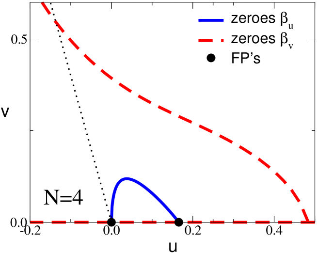
Figure 1: Zeroes of the $3d$-$\overline{\rm MS}$ $\beta$-functions for $N=4$ in the region $v>0$ (solid line for $\beta_{u}$, dashed line for $\beta_{v}$). The black dots indicate the Gaussian and the O(20) FPs. The dotted line $4u+v=0$ separates the Borel-summable region (at the right) from the non-Borel-summable region (at the left).

The analysis of the six-loop MZM series was done in a similar way. We considered the functions $\beta_{u}(u,v)/u$ and $\beta_{v}(u,v)/v$ and we apply the conformal-mapping method as before. The results are perfectly consistent with the $3d$-$\overline{\rm MS}$ ones. No additional FP is found for $N=4$.

According to our FT results, a consistent model for a three-dimensional continuous transition characterized by a complex symmetric $N\times N$ matrix order parameter and symmetry-breaking pattern ${\rm U}(N)\rightarrow{\rm O}(N)$ does not exist for $N=4$. Therefore, the phase transition in such systems must be of first order. For $N=2$ instead, there is a stable FP; thus, systems characterized by the symmetry breaking U(2)$\rightarrow$ O(2) can undergo a continuous transition, if they are in the attraction domain of the stable FP.

4 Renormalization-group flow of the SU($N$) LGW theory

We now study the effect of the breaking of ${\rm U}(1)_{A}$. As we mentioned in Sec. 2, we must add to the U($N$) Lagrangian a term proportional to ${\rm det}\,\Phi+{\rm det}\,\Phi^{\dagger}$. Such a term is irrelevant for $N>4$: in this case the critical behavior is described by the U($N$) theory. Therefore, we only consider the cases $N=2$ and $N=4$, which are the only ones of interest for aQCD. Indeed, $N>4$ corresponds to $N_{f}>2$ and aQCD is asymptotically free only for $N_{f}<11/4=2.75$.

4.1 The case $N=2$

In the case $N=2$ ($N_{f}=1$), the determinant is quadratic in the fundamental field $\Phi$, and other terms must be added to the effective Lagrangian, i.e. all possible interactions with at most four fields. This leads to the LGW Lagrangian

$${\cal L}_{SU(2)}={\rm Tr}\,(\partial_{\mu}\Phi^{\dagger})(\partial_{\mu}\Phi)+r{\rm Tr}\,\Phi^{\dagger}\Phi+w_{0}\left({\rm det}\,\Phi^{\dagger}+{\rm det}\,\Phi\right)+{u_{0}\over 4}\left({\rm Tr}\,\Phi^{\dagger}\Phi\right)^{2}$$

$$+{v_{0}\over 4}{\rm Tr}\left(\Phi^{\dagger}\Phi\right)^{2}+{x_{0}\over 4}\left({\rm Tr}\,\Phi^{\dagger}\Phi\right)\left({\rm det}\,\Phi^{\dagger}+{\rm det}\,\Phi\right)+{y_{0}\over 4}\left[({\rm det}\,\Phi^{\dagger})^{2}+({\rm det}\,\Phi)^{2}\right],$$ (29)

where $\Phi_{ij}$ is a complex symmetric 2$\times$2 matrix. Note that there is no need to include also a term proportional to $({\rm det}\,\Phi)({\rm det}\,\Phi^{\dagger})$. Indeed, for any two dimensional matrix $M$, we have $2\,{\rm det}\,M=({\rm Tr}\,M)^{2}-{\rm Tr}\,M^{2}$. Therefore,

$$2({\rm det}\,\Phi)({\rm det}\,\Phi^{\dagger})=\left({\rm Tr}\,\Phi^{\dagger}\Phi\right)^{2}-{\rm Tr}\left(\Phi^{\dagger}\Phi\right)^{2}.$$ (30)

Since the Lagrangian (29) has two quadratic mass terms, it describes several transition lines with a multicritical point.

Model (29) can be written in terms of two real three-component fields $\phi_{i}$ and $\varphi_{i}$ by writing $\Phi=\sum_{j=1}^{3}(\phi_{j}+i\varphi_{j})e_{j}$, where $(e_{1},e_{2},e_{3})\equiv({\rm Id}/2,i\sigma_{1}/2,i\sigma_{3}/2)$, ${\rm Id}$ is the $2\times 2$ identity matrix, and $\sigma_{i}$ are the Pauli matrices. One obtains

$${\cal L}_{\phi\varphi} = {1\over 2}(\partial_{\mu}\phi)^{2}+{1\over 2}(\partial_{\mu}\varphi)^{2}+{r_{\phi}\over 2}\phi^{2}+{r_{\varphi}\over 2}\varphi^{2}$$ (31)

$$+{a_{0}\over 4!}(\phi^{2})^{2}+{b_{0}\over 4!}(\varphi^{2})^{2}+{c_{0}\over 4!}\phi^{2}\varphi^{2}+{d_{0}\over 4!}(\phi\cdot\varphi)^{2},$$

with $r_{\phi}=r+w_{0}$, $r_{\varphi}=r-w_{0}$, $a_{0}=\frac{3}{4}(2u_{0}+v_{0}+2x_{0}+y_{0})$, $b_{0}=\frac{3}{4}(2u_{0}+v_{0}-2x_{0}+y_{0})$, $c_{0}=\frac{3}{2}(2u_{0}+3v_{0}-y_{0})$, and $d_{0}=-3(v_{0}+y_{0})$. The mean-field phase diagram of such a model is studied in Ref. [50]. One finds a multicritical point with several transition lines. The analysis reported in Ref. [50] indicates that the multicritical point may either belong to the chiral ${\rm O(2)}\otimes{\rm O(3)}$ universality class or may correspond to a first-order transition. Note that in Ref. [50] the full RG flow was not studied and thus one cannot exclude the presence of other stable FPs, beside the ${\rm O(2)}\otimes{\rm O(3)}$ chiral FP. This possibility is rather unlikely, but an explicit calculation of the RG flow in the full parameter space is needed to settle the question. Here, we will not consider this additional possibility, since it is of no relevance for aQCD, as we discuss below. In the plane $t$, $g$, where $g$ parametrizes the breaking of the symmetry $\phi\leftrightarrow\varphi$, the possible phase diagrams are reported in Fig. 2.

Figure 2: Possible phase diagrams for model (31). In phase diagrams (a1), (a2), and (a3) the multicritical point corresponds to a second-order transition, while in phase diagrams (b1), (b2), and (b3) the multicritical transition is of first order. Thick lines represent first-order transition, while thin lines correspond to second-order transitions. We label with H, XY, and Is the lines corresponding to transitions belonging to the Heisenberg ($N=3$ vector), XY ($N=2$ vector), and Ising universality classes, respectively.

In the case of one-flavor aQCD, the U(2) theory obtained by setting $w_{0}=0$, $x_{0}=0$, $y_{0}=0$ should correspond to the multicritical point because of the larger symmetry group. Therefore, the relevant FP at the multicritical point is the one found for the U(2) theory in Sec. 3.3. The other FPs of the theory (31) are of no relevance since they are not present in the U(2) model. Thus, if chiral symmetry is not restored at the transition, the behavior of aQCD as a function of temperature $T$ corresponds to the behavior observed along a nontrivial line in the $(t,g)$ plane in one of the phase diagrams reported in Fig. 2.  However, we do not know which of the phase diagrams applies. Generically, we expect two phase transitions. One of them, that should occur at higher values of $T$, may be either of first order or belong to the Heisenberg universality class [whose symmetry-breaking pattern is SO(3)$\to$SO(2)], which has been accurately studied in the literature, see, e.g., Refs. [51, 27] and references therein. Such a transition would be associated with the symmetry breaking ${\mathbb{Z}}_{2}\otimes{\rm SU(2)}\to{\mathbb{Z}}_{2}\otimes{\rm O}(2)$. The lower-temperature transition, that may not necessarily exist, may be of first order, or continuous. According to Fig. 2, the transition may belong either to the Ising or to the XY universality class. It is easy to see that in the latter case the U(1)_V symmetry would be broken, violating the Vafa-Witten theorem [6]. Therefore, the only possibility is an Ising transition that corresponds to the breaking ${\mathbb{Z}}_{2}\otimes{\rm O}(2)\to{\mathbb{Z}}_{2}\otimes{\rm SO}(2)$. Note that the symmetry breaking ${\rm SU}(2)\to{\rm SO}(2)$ is realized here through two different transitions and that an SU(2)/SO(2) universality class does not exist. One may discriminate between the one- or two-transition hypothesis by determining the symmetry of the $T=0$ phase, which differs by a ${\mathbb{Z}}_{2}$ group in the two cases.

4.2 The case $N=4$

For $N=4$ ($N_{f}=2$) the determinant is a quartic-order term, giving rise to a generalized LGW $\Phi^{4}$ theory (5) with three quartic parameters. In this case stability requires

$$u_{0}+v_{0}\geq 0,\qquad 4u_{0}+v_{0}-2|w_{0}|\geq 0.$$ (32)

As discussed in the Appendix, the symmetry-breaking pattern and vacuum structure appropriate for aQCD are realized for $v_{0}>-{3\over 2}|w_{0}|$. Note that the FPs already identified in the ${\rm U}(4)$ theory, i.e. the Gaussian and the O(20) FP, are also FPs of the ${\rm SU}(4)$ theory. They are both unstable and thus are of no relevance for the critical behavior.

In order to study the RG flow of the theory (5) for $N=4$, we consider the $3d$-$\overline{\rm MS}$ scheme and the MZM scheme as before. In the $3d$-$\overline{\rm MS}$ scheme we set

$$\Phi = [Z_{\phi}(u,v,w)]^{1/2}\Phi_{R},$$ (33)

$$u_{0} = A_{d}\mu^{\epsilon}Z_{u}(u,v,w),$$

$$v_{0} = A_{d}\mu^{\epsilon}Z_{v}(u,v,w),$$

$$w_{0} = {1\over 24}A_{d}\mu^{\epsilon}Z_{w}(u,v,w),$$

and determine the corresponding $\beta$ functions to five loops. They are given by

$$\beta_{u} = -\epsilon u+7u^{2}+5uv+\frac{3}{4}v^{2}+3w^{2}-\frac{111}{8}u^{3}-\frac{55}{4}u^{2}v-\frac{29}{4}uv^{2}$$

$$-\frac{9}{4}v^{3}-\frac{33}{2}uw^{2}-3vw^{2}+\sum_{i+j+k\geq 4}c^{u}_{ijk}u^{i}v^{j}w^{k},$$

$$\beta_{v} = -\epsilon v+3uv+\frac{13}{4}v^{2}-3w^{2}-\frac{91}{8}u^{2}v-16uv^{2}-6v^{3}$$

$$+9uw^{2}+\frac{9}{2}vw^{2}+\sum_{i+j+k\geq 4}c^{v}_{ijk}u^{i}v^{j}w^{k},$$

$$\beta_{w} = -\epsilon w+3uw-\frac{3}{2}vw-\frac{91}{8}u^{2}w-\frac{7}{4}v^{2}w-\frac{7}{4}uvw$$

$$+\frac{3}{2}w^{3}+\sum_{i+j+k\geq 4}c^{w}_{ijk}u^{i}v^{j}w^{k}.$$

The coefficients $c_{ijk}$ up to five loops, i.e. for $4\leq i+j+k\leq 6$, are reported in Table 5. We also computed the five-loop expansion of the RG functions $\eta_{\phi,t}$ defined as in Eq. (10):

$$\eta_{\phi,t}=\sum_{i+j+k\geq 1}e^{\phi,t}_{ijk}u^{i}v^{j}w^{k}\;.$$ (37)

The coefficients $e^{\phi}_{ijk}$ and $e^{t}_{ijk}$ up to five loops, i.e. for $1\leq i+j+k\leq 5$, are reported in Table 6. The standard critical exponents are related to $\eta_{\phi,t}$ by

$$\eta=\eta_{\phi}(u^{*},v^{*},w^{*}),\qquad\nu=\left[2+\eta_{t}(u^{*},v^{*},w^{*})-\eta_{\phi}(u^{*},v^{*},w^{*})\right]^{-1},$$ (38)

where $u^{*}$, $v^{*}$, $w^{*}$ are the coordinates of the stable FP in the case it exists.

In the MZM scheme, beside the renormalization conditions (14) and (15), we also set

$$\hat{\Gamma}^{(4)}_{a_{1}a_{2},b_{1}b_{2},c_{1}c_{2},d_{1}d_{2}}(0) = \left.{\delta^{4}\Gamma\over\delta\Phi_{a_{1}a_{2}}\delta\Phi_{b_{1}b_{2}}\delta\Phi_{c_{1}c_{2}}\delta\Phi_{d_{1}d_{2}}}\right|_{\rm zero\;mom.}$$ (39)

$$= Z_{\phi}^{-2}m^{4-d}{\pi\over 21}w\epsilon_{a_{1}b_{1}c_{1}d_{1}}\epsilon_{a_{2}b_{2}c_{2}d_{2}},$$

where $\epsilon_{ijkl}$ is the completely antisymmetric tensor ($\epsilon_{1234}=1$). We computed six-loop series in the MZM scheme. The MZM $\beta$ functions are given by

$$\beta_{u} = -u+u^{2}+\frac{5}{7}uv+\frac{3}{28}v^{2}+\frac{3}{7}w^{2}+\sum_{i+j+k\geq 3}d^{u}_{ijk}u^{i}v^{j}w^{k},$$ (40)

$$\beta_{v} = -v+\frac{3}{7}uv+\frac{13}{28}v^{2}-\frac{3}{7}w^{2}+\sum_{i+j+k\geq 3}d^{v}_{ijk}u^{i}v^{j}w^{k},$$ (41)

$$\beta_{w} = -w+\frac{3}{7}uw-\frac{3}{14}vw+\sum_{i+j+k\geq 3}d^{w}_{ijk}u^{i}v^{j}w^{k}.$$ (42)

The coefficients $d_{ijk}$ up to six loops, i.e. for $3\leq i+j+k\leq 7$, are reported in Table 7. We also computed the RG functions $\eta_{\phi,t}$ defined in Eq. (18) to six loops. The coefficients $e^{\phi}_{ijk}$ and $e^{t}_{ijk}$ defined in Eq. (37) are reported in Table 6.

Again, close to four dimensions there are only two FPs, the Gaussian and the O(20) FPs (the latter located at $u=\epsilon/7$, $v=0$, and $w=0$), i.e. those already found in the U(4) theory, which are both unstable. In order to investigate the possible existence of other FPs in three dimensions, we analyze the $3d$-$\overline{\rm MS}$ and MZM perturbative expansions. Note that the model is invariant under the transformations $\Phi\to e^{i\pi/4}\Phi$, $(u,v,w)\to(u,v,-w)$. This implies that $\beta_{u}$, $\beta_{v}$, and $\beta_{w}/w$ are even in $w$. Therefore, we can restrict our search of FPs to the $w>0$ space; if a FP with coordinates $u,v,w>0$ exists, there is also another FP with the same critical properties at $u,v,-w$.

We use the conformal-mapping method already employed in Sec. 3.3 and the large-order behavior of the perturbative series. Writing

$$S(xu,xv,xw)=\sum_{n}s_{n}(u,v,w)x^{n},$$ (43)

semiclassical calculations based on instanton solutions give

$$s_{n}\sim n![-A(u,v,w)]^{n}\,n^{b},$$ (44)

$$A(u,v,w)=c\,{\rm Max}\left(u+v,\,u+\frac{v}{4}+\frac{|w|}{2}\right),$$

where the constant $c$ is given by $c=3/4$ and $c=0.0474989$ respectively for the $\overline{\rm MS}$ and MZM expansions. The perturbative expansions are Borel summable for

$$u+v\geq 0,\qquad 4u+v-2|w|\geq 0\;.$$ (45)

The $3d$-$\overline{\rm MS}$ five-loop series are analyzed as in the U($N$) case and indicate the presence of a new FP with $w\not=0$. Most approximants of the five-loop series (more than 90% of the approximants with $\alpha=-1,0,1,2$ and $b=3,\ldots,18$) present a common zero with $w>0$. They are approximately 50% at four loops. This new FP is located at $u^{*}=0.23(9)$, $v^{*}=0.34(6)$, and $w^{*}=0.54(8)$, where the error takes into account the spread of the results of the approximants considered. Note that the error (spread of the results) is rather large, essentially because this FP lies relatively far from the origin (note that the O(20) FP lies at $u^{*}\approx 0.17$), and also because it is close to the boundary of the Borel summable region. The analysis of the corresponding stability matrix shows that this FP is stable, and therefore it determines the universal properties of continuous transitions in systems described by the SU(4) LGW $\Phi^{4}$ theory (5). We also computed the corresponding critical exponents by evaluating the RG functions $\eta_{\phi,t}$ at the FP. From the analysis of the expansions of $\eta_{\phi}$ and $(2+\eta_{t}-\eta_{\phi})^{-1}$, we obtain $\eta=0.23(8)$ and $\nu=1.1(3)$, where the error takes into account the spread of the approximants and the uncertainty on the FP coordinates. The presence of the stable FP is confirmed by an analysis based on Padé-Borel approximants; indeed, using [4/1] Padé approximants for all $\beta$ functions, one obtains $u^{*}\approx 0.29(5)$, $v^{*}\approx 0.23(1)$, and $w^{*}\approx 0.51(4)$ (the errors indicate how the results change when the parameter $b$ is varied between 4 and 18), which is substantially consistent with the results of the conformal-mapping analysis. Apparently, the Padé-Borel method gives a more accurate estimate of the location of the FP. But, note that the error is only related to the dependence on $b$ of a single Padé approximant; thus, it is likely to be underestimated. As we have already seen in many other instances, the conformal-method error should provide a more realistic estimate of the real accuracy of the result.

The rather low precision of the $3d$-$\overline{\rm MS}$ results may give rise to some doubts on the existence itself of the stable FP, and therefore it calls for an independent and nontrivial crosscheck. This is provided by the analysis of the perturbative expansions in the alternative three-dimensional MZM scheme. We follow the same steps as in the U($N$) case, considering the conformal-mapping method and approximants with $\alpha=-1,0,1,2$ and $b=3,...18$ (see Ref. [49] for definitions). The analysis confirms the presence of a stable FP at $u^{*}=0.0(3)$, $v^{*}=3.5(2)$ and $w^{*}=4.6(2)$, where the error is related to the spread of the results. The presence of a FP is stable with respect to the number of loops. Indeed, at five loops (resp. four loops) we find a FP at $u^{*}=0.4(2)$, $v^{*}=3.2(2)$ and $w^{*}=4.3(2)$ (resp. $u^{*}=0.7(3)$, $v^{*}=3.6(5)$ and $w^{*}=4.6(6)$). For comparison, in this scheme the O(20) FP is located at $u^{*}\approx 1.18$ [32]. We also estimate the critical exponents, finding $\eta=0.20(3)$ and $\nu=1.1(3)$ (again from the analysis of the expansions of $\eta_{\phi}$ and $(2+\eta_{t}-\eta_{\phi})^{-1}$), in substantial agreement with the results of the $3d$-$\overline{\rm MS}$ scheme. Also in this scheme results are not very precise, although they are apparently more accurate than the $3d$-$\overline{\rm MS}$ ones.

In conclusion, the analysis of the perturbative expansions in the 3$d$-$\overline{\rm MS}$ and MZM schemes provides evidence for the existence of a stable FP, and therefore of a new universality class that describes continuous transitions in systems described by the LGW Lagrangian (5) with $N=4$ and symmetry-breaking pattern ${\rm SU(4)}\to{\rm SO(4)}$. Although the results of the analyses do not appear particularly precise, the substantial agreement between the two schemes makes us confident on their reliability. Note that the existence of a FP does not exclude the possibility of observing first-order transitions; indeed, this is still possible for systems outside the attraction domain of the stable FP.

We recall that in Sec. 3.3 we found no stable FP in the U(4) LGW $\Phi^{4}$ theory, which should be relevant if the U(1) symmetry broken by the anomaly is effectively restored at $T_{c}$, thus suggesting first-order transitions for the corresponding systems. The existence of a stable FP with $w\not=0$ in the SU(4) theory is an interesting example of the so-called phenomenon of softening of first-order transitions: by breaking some symmetry of the original model, a first-order transition may become a second-order one. This phenomenon is well known in spin systems: the introduction of quenched disorder may soften the first-order transitions of pure systems [52]. In disordered systems translational invariance is the broken symmetry. In our case, it is instead the internal symmetry of the system that gets reduced.

Appendix A Vacua of the U($N$) and SU(4) theories

Let us consider the potential

$$V_{U(N)}(\Phi)=r{\rm Tr}\,\Phi^{\dagger}\Phi+{u_{0}\over 4}\left({\rm Tr}\,\Phi^{\dagger}\Phi\right)^{2}+{v_{0}\over 4}{\rm Tr}\left(\Phi^{\dagger}\Phi\right)^{2},$$ (46)

and let us determine the fields that minimize it. The stationarity condition gives the equation

$$r\Phi_{ab}+{u_{0}\over 2}\Phi_{ab}{\rm Tr}\,\Phi^{\dagger}\Phi+{v_{0}\over 2}\left(\Phi\Phi^{\dagger}\Phi\right)_{ab}=0.$$ (47)

If $\Phi$ is a solution of Eq. (47), it is easy to show that

$$\left.V_{U(N)}(\Phi)\right|_{\rm sol}={r\over 2}{\rm Tr}\,\Phi^{\dagger}\Phi.$$ (48)

In order to determine the solutions of Eq. (47), let us perform a polar decomposition of $\Phi$: we write $\Phi=PU$, where $P=\sqrt{\Phi^{\dagger}\Phi}$ is a hermitian positive semidefinite matrix and $U$ is a unitary matrix. Then we diagonalize $P$, writing $P=VP_{d}V^{\dagger}$ with $P_{d}={\rm diag}(\lambda_{1},\lambda_{2},\ldots,\lambda_{N})$, $\lambda_{1}\geq\lambda_{2}\geq\ldots\geq\lambda_{N}\geq 0$, and $V$ unitary. Now, if $k$ is the rank of $\Phi$, we have for $1\leq a\leq k$ the equation

$$r+{u_{0}\over 2}{\rm Tr}\,P^{2}_{d}+{v_{0}\over 2}\lambda_{a}^{2}=0,$$ (49)

that shows that $\lambda_{a}$ does not depend on $a$. Summing this equation over $1\leq a\leq k$, we obtain

$${\rm Tr}\,\Phi^{\dagger}\Phi={\rm Tr}\,P^{2}_{d}=\sum_{a=1}^{k}\lambda_{a}^{2}=-{2kr\over ku_{0}+v_{0}}.$$ (50)

Since $u_{0}+v_{0}>0$ and $Nu_{0}+v_{0}>0$, for $r>0$ we must have $k=0$, i.e. the only possible solution is $\Phi=0$: for $r>0$ the system is disordered. For $r<0$ instead, any $k$ with $0\leq k\leq N$ is acceptable. Using Eq. (48) we obtain

$$\left.V(\Phi)\right|_{\rm sol}=-{kr^{2}\over ku_{0}+v_{0}},$$ (51)

which shows that the energy depends only on the rank $k$ of the solution. A simple calculation shows that the minimum of the potential is attained for $k=N$ if $v_{0}>0$ and $k=1$ if $v_{0}<0$.

For $k=N$, we have

$$P=-{2r\over Nu_{0}+v_{0}}\,{\rm Id},$$ (52)

where $\rm Id$ is the identity matrix. Thus, $\Phi\propto Q$, where $Q$ is a symmetric unitary matrix. Of course, being U($N$) connected, we can write $Q=U^{2}=UU^{T}$, with $U$ unitary and symmetric. Thus, modulo symmetry transformations, we may take $\Phi_{\rm min}\propto{\rm Id}$.

If $k=1$, $\Phi_{ab}=v_{a}v_{b}$, where $v_{a}$ is an $N$-dimensional complex vector. Since, for any $v$ there exists $U\in{\rm U}(N)$ such that $v_{a}=\sum_{b}U_{ab}w_{b}$, where $w=(a,0,\ldots,0)$, with $a$ real and positive, we can write $\Phi$ as

$$\Phi=-{2r\over u_{0}+v_{0}}UI_{1}U^{T},$$ (53)

with $I_{1}={\rm diag}(1,0,\ldots,0)$. Thus, modulo symmetry transformations, we may take $\Phi_{\rm min}\propto{\rm I_{1}}$.

Let us now determine the symmetry-breaking patterns. The theory is invariant under the transformations $\Phi\to U\Phi U^{T}$, $U$ unitary, which form a group isomorphic to U($N)/{\mathbb{Z}}_{2}$ (the quotient is due to the fact that $U$ and $-U$ give rise to the same transformation). The transformations that leave invariant $\Phi_{\rm min}\propto{\rm Id}$ are those with $U\in{\rm O}(N)$, so that the invariance group is ${\rm O}(N)/{\mathbb{Z}}_{2}$. If $\Phi_{\rm min}\propto{\rm I_{1}}$, the transformations that leave invariant $\Phi_{\rm min}$ have the form $U=(\pm 1)\oplus R$, $R\in{\rm U}(N-1)$, so that the invariance group is $[{\rm U}(N-1)\otimes{\mathbb{Z}}_{2}]/{\mathbb{Z}}_{2}\cong{\rm U}(N-1)$. Beside $\Phi\to U\Phi U^{T}$, the model, ${\rm Id}$, and $I_{1}$ are invariant under the ${\mathbb{Z}}_{2}$ transformations $\Phi\to\Phi^{\dagger}$. Thus, the symmetry breaking pattern is ${\rm U}(N)\to{\rm O}(N)$ for $v_{0}>0$ and ${\rm U}(N)\to{\rm U}(N-1)\otimes{\mathbb{Z}}_{2}$ for $v_{0}<0$. Note that for $N=2$ they are identical since ${\rm O}(2)\cong{\rm SO}(2)\otimes{\mathbb{Z}}_{2}\cong{\rm U}(1)\otimes{\mathbb{Z}}_{2}$.

To conclude, let us note that, as a consequence of the Vafa-Witten theorem [6], the vector group $U(N_{f})_{V}$ can never be broken. Therefore, the vacuum must be invariant under the $U(N/2)$ transformations

$$U_{V}\equiv\left(\begin{array}[]{cc}U&0\\ 0&U^{*}\end{array}\right),$$ (54)

with $U\in U(N/2)$. It is easy to verify that the only symmetric matrices $Q$ such that $U_{V}QU_{V}^{T}=Q$ are proportional to

$$J\equiv\left(\begin{array}[]{cc}0&{\rm Id}\\ {\rm Id}&0\end{array}\right)\;,$$ (56)

where ${\rm Id}$ is the $N/2\times N/2$ identity matrix. Thus, the only possible vacuum for aQCD is proportional to $J$. It is easy to verify that this is possible for $v>0$ (as we showed any matrix proportional to a symmetric unitary matrix is a possible vacuum), but not for $v<0$. Thus, in the aQCD case we must restrict ourselves to the case $v>0$.

Now let us consider the effect of the determinant for $N=4$. The potential is

$$V_{SU(N)}(\Phi)=V_{U(N)}(\Phi)+w_{0}({\rm det}\,\Phi+{\rm det}\,\Phi^{\dagger}).$$ (57)

The stationarity condition gives then

$$r\Phi_{ab}+{u_{0}\over 2}\Phi_{ab}{\rm Tr}\,\Phi^{\dagger}\Phi+{v_{0}\over 2}(\Phi\Phi^{\dagger}\Phi)_{ab}+{w_{0}\over 6}\sum_{c_{1}d_{1}e_{1}c_{2}d_{2}e_{2}}\epsilon_{bc_{1}d_{1}e_{1}}\epsilon_{ac_{2}d_{2}e_{2}}\Phi_{c_{1}c_{2}}^{\dagger}\Phi_{d_{1}d_{2}}^{\dagger}\Phi_{e_{1}e_{2}}^{\dagger}=0.$$ (58)

Now, we write again $\Phi=VP_{d}V^{\dagger}U=\hat{V}P_{d}[({\rm det}\,V)^{1/2}V^{\dagger}UV^{*}]\hat{V}^{T}$ with $P_{d}$ diagonal and $\hat{V}=V({\rm det}\,V)^{-1/4}$. Thus, modulo a symmetry transformation, we can simply write $\Phi=P_{d}U$, with $U$ unitary. Substituting in the previous equation we obtain the equation

$$r\lambda_{a}+{u_{0}\over 2}\lambda_{a}{\rm Tr}\,P_{d}^{2}+{v_{0}\over 2}\lambda_{a}^{3}-w_{0}({\rm det}\,U)\prod_{c\not=a}\lambda_{c}=0.$$ (59)

The term proportional to $w_{0}$ is the product of three eigenvalues and thus it is relevant only if the rank of $\Phi$ is 3 or 4. If the rank is three, assume $\lambda_{4}=0$. The previous equation for $a=4$ gives

$$\lambda_{1}\lambda_{2}\lambda_{3}=0,$$ (60)

that contradicts the hypothesis $\lambda_{1}\lambda_{2}\lambda_{3}\not=0$. Thus, there is no solution with rank $k=3$.

Assume now that the rank $k$ is 4. Since all $\lambda_{a}$ are real and nonvanishing, $({\rm det}\,U)$ must be real, hence equal to $s=\pm 1$, since $U$ is unitary. Let us now determine the eigenvalues. Eq. (59) implies

$$R_{ab}\equiv\lambda_{a}E_{a}-\lambda_{b}E_{b}=(\lambda_{a}^{2}-\lambda_{b}^{2})\left[r+{u_{0}\over 2}{\rm Tr}\,P_{d}^{2}+{v_{0}\over 2}(\lambda_{a}^{2}+\lambda_{b}^{2})\right]=0.$$ (61)

Now, consider $R_{12}=0$, $R_{13}=0$, and $R_{23}=0$. It is immediate to verify that these equations imply that at least two eigenvalues among $\lambda_{1}$, $\lambda_{2}$, $\lambda_{3}$ are equal. Without loss of generality we assume $\lambda_{1}=\lambda_{2}$. An analogous discussion indicates that at least two eigenvalues among $\lambda_{1}$, $\lambda_{3}$, $\lambda_{4}$ are equal. Thus, there are two possible cases: $\lambda_{1}=\lambda_{2}=\lambda_{3}$; $\lambda_{1}=\lambda_{2}$ and $\lambda_{3}=\lambda_{4}$. Finally, consider $R_{24}=0$; we obtain that either $\lambda_{2}=\lambda_{4}$ or $2r+{u_{0}}{\rm Tr}\,P_{d}^{2}+{v_{0}}(\lambda_{2}^{2}+\lambda_{4}^{2})=0$, that gives a relation between $\lambda_{2}$ and $\lambda_{4}$. In conclusion, we obtain two different classes of solutions:

• all eigenvalues are equal with

  $$\lambda^{2}_{a}={-2r\over 4u_{0}+v_{0}+2sw_{0}}$$ (62)

  and potential

  $$\left.V(\Phi)\right|_{\rm sol}={-4r^{2}\over 4u_{0}+v_{0}+2sw_{0}};$$ (63)

• one eigenvalue differs from the others:

  $$\lambda_{1}^{2}=\lambda_{2}^{2}=\lambda_{3}^{2}={-2rv_{0}^{2}\over 3u_{0}v_{0}^{2}+v_{0}^{3}+4u_{0}w_{0}^{2}+4v_{0}w_{0}^{2}},$$

  $$\lambda_{4}={2sw_{0}\over v_{0}}\lambda_{1},$$ (64)

  with potential

  $$\left.V(\Phi)\right|_{\rm sol}=-r^{2}{3v_{0}^{2}+4w_{0}^{2}\over 3u_{0}v_{0}^{2}+v_{0}^{3}+4u_{0}w_{0}^{2}+4v_{0}w_{0}^{2}}.$$ (65)

  Note that the solution with $s=1$ exists only if $w_{0}v_{0}$ is positive, the one with $s=-1$ in the opposite case. For $w_{0}=0$ this solution corresponds to the rank-3 solution we have determined before.

Comparing the value of the potential for the different solutions, we obtain finally:

• for $v_{0}<0$ and $|w_{0}|<-2v_{0}/3$ the relevant solution has rank $k=1$ and thus, modulo symmetry transformations, we can take $\Phi_{\rm min}\propto I_{1}$. The symmetry of the vacuum is SU(3)$\otimes{\mathbb{Z}}_{2}$. Such a case is not of interest for aQCD, since it is not invariant under U(2)_V.

• for $w_{0}>0$ and $w_{0}>-2v_{0}/3$ the relevant solution is given by Eq. (62) with potential (63), setting $s=-1$. Therefore, $U$ is symmetric with ${\rm det}\,U=-1$. It follows that $U=e^{i\pi/4}VV^{T}$, $V\in{\rm SU}(4)$. Modulo symmetry transformations, one can therefore choose $\Phi_{\rm min}\propto e^{i\pi/4}{\rm Id}$. The vacuum is invariant under ${\rm SO(4)}$ (note that the symmetry $\Phi\to\Phi^{\dagger}$ is broken here). This case is not relevant for aQCD since the vacuum breaks $\Phi\to\Phi^{\dagger}$.

• for $w_{0}<0$ and $|w_{0}|>-2v_{0}/3$ the relevant solution is given in Eq. (62) with potential (63), setting $s=1$. Therefore, $U$ is symmetric with ${\rm det}\,U=1$. It follows that $U=VV^{T}$ with $V\in$ SU(4). Modulo symmetry transformations, one can therefore choose $\Phi_{\rm min}\propto{\rm Id}$. The vacuum is invariant under ${\rm SO(4)}\otimes{\mathbb{Z}}_{2}$. The matrix $J$ is one of the possible vacuum solutions and thus this case is of relevance for aQCD.

Table 1: $3d$-$\overline{\rm MS}$ scheme: coefficients $a^{u}_{ij}$, cf. Eq. (3.1).

$i,j$	$a^{u}_{ij}$
4,0	$10.7397+2.92770N+2.99216N^{2}+0.128906N^{3}+0.0644531N^{4}$
3,1	$17.5092+18.1264N+1.23437N^{2}+0.617187N^{3}$
2,2	$25.2599+9.50698N+3.95252N^{2}+0.0117187N^{3}+0.00292968N^{4}$
1,3	$13.4014+8.45267N+0.626953N^{2}+0.117187N^{3}$
0,4	$3.61949+1.54627N+0.301169N^{2}$
5,0	$-63.5743-21.0606N-22.3638N^{2}-2.60592N^{3}-1.30194N^{4}$
	$+0.00122070N^{5}+0.000406901N^{6}$
4,1	$-140.774-153.387N-25.2352N^{2}-12.6425N^{3}-0.0298321N^{4}$
	$-0.00994404N^{5}$
3,2	$-260.744-143.388N-66.5772N^{2}-2.01164N^{3}-0.526260N^{4}$
2,3	$-212.910-157.262N-23.2253N^{2}-5.14407N^{3}-0.0223761N^{4}$
	$-0.00344248N^{5}$
1,4	$-107.874-60.8991N-15.9106N^{2}-0.709064N^{3}-0.0784548N^{4}$
0,5	$-20.6853-12.8827N-2.21799N^{2}-0.215929N^{3}$
6,0	$475.552+183.011N+200.1526N^{2}+34.5561N^{3}+17.9613N^{4}+0.818270N^{5}$
	$+0.269906N^{6}-0.00244287N^{7}-0.000610718N^{8}$
5,1	$1339.84+1524.75N+373.269N^{2}+195.251N^{3}+10.3200N^{4}+3.40600N^{5}$
	$-0.0291545N^{6}-0.00728864N^{7}$
4,2	$3025.04+2080.71N+1065.77N^{2}+97.1136N^{3}+29.0928N^{4}+0.178866N^{5}$
	$+0.0283466N^{6}$
3,3	$3355.06+2824.44N+654.568N^{2}+172.564N^{3}+4.47104N^{4}+0.769792N^{5}$
2,4	$2471.77+1715.81N+548.534N^{2}+48.2367N^{3}+6.77586N^{4}+0.0200149N^{5}$
	$+0.00195671N^{6}$
1,5	$944.177+692.287N+168.563N^{2}+25.2091N^{3}+0.760372N^{4}+0.0526262N^{5}$
0,6	$157.642+109.278N+29.0944N^{2}+2.78840N^{3}+0.163781N^{4}$

Table 2: $3d$-$\overline{\rm MS}$ scheme: coefficients $a^{v}_{ij}$, cf. Eq. (3.1).

$i,j$	$a^{v}_{ij}$
4,0	$0$
3,1	$25.4497+2.33904N+2.288N^{2}-0.101562N^{3}-0.0507812N^{4}$
2,2	$39.1784+23.3634N-0.0214843N^{2}-0.136718N^{3}$
1,3	$29.5574+12.9326N+2.32341N^{2}$
0,4	$7.12024+3.75368N+0.486716N^{2}+0.0253906N^{3}$
5,0	$0$
4,1	$-177.097-22.3032N-22.5027N^{2}-0.392090N^{3}-0.178529N^{4}$
	$+0.0210195N^{5}+0.00700652N^{6}$
3,2	$-374.999-241.790N-14.5218N^{2}-4.72881N^{3}+0.179072N^{4}+0.0584779N^{5}$
2,3	$-422.833-232.645N-55.3180N^{2}+0.1763229N^{3}+0.137500N^{4}$
1,4	$-209.997-132.747N-23.9377N^{2}-2.37050N^{3}$
0,5	$-42.8890-25.8808N-5.72264N^{2}-0.396930N^{3}-0.0136094N^{4}$
6,0	$0$
5,1	$1513.47+243.234N+250.177N^{2}+13.8095N^{3}+6.71436N^{4}$
	$-0.228540N^{5}-0.0762733N^{6}-0.0000799564N^{7}-0.0000199891N^{8}$
4,2	$4108.25+2830.72N+327.369N^{2}+121.934N^{3}-0.955058N^{4}$
	$-0.471074N^{5}-0.00569730N^{6}-0.00109038N^{7}$
3,3	$6155.99+3929.91N+1110.53N^{2}+33.3855N^{3}+4.60723N^{4}$
	$+0.0693464N^{5}+0.00888516N^{6}$
2,4	$4661.51+3367.08N+766.260N^{2}+98.8345N^{3}-0.0328212N^{4}-0.0247545N^{5}$
1,5	$1909.14+1333.31N+360.926N^{2}+37.1082N^{3}+2.38066N^{4}$
0,6	$317.910+228.597N+59.1341N^{2}+7.38414N^{3}+0.318597N^{4}+0.00727653N^{5}$

Table 3: MZM scheme: coefficients $b^{u}_{ij}$, cf. Eq. (19).

$i,j$	$(N^{2}+N+8)^{i+j-1}\,b^{u}_{ij}$
$3$,$0$	$-28.1481-6.07407\,N-6.07407\,N^{2}$
$2$,$1$	$-29.6296-29.6296\,N$
$1$,$2$	$-30.8148-5.11111\,N-1.7037\,N^{2}$
$0$,$3$	$-8-4N$
$4$,$0$	$199.64+54.9404\,N+56.2893\,N^{2}+2.69789\,N^{3}+1.34894\,N^{4}$
$3$,$1$	$329.228+342.521\,N+26.5875\,N^{2}+13.2938\,N^{3}$
$2$,$2$	$476.927+191.216\,N+81.4672\,N^{2}+1.24378\,N^{3}+0.310945\,N^{4}$
$1$,$3$	$254.359+165.976\,N+16.1265\,N^{2}+3.27131\,N^{3}$
$0$,$4$	$68.2248+29.746\,N+5.95053\,N^{2}$
$5$,$0$	$-1832.21-602.521\,N-638.341\,N^{2}-71.4848\,N^{3}-35.3533\,N^{4}+0.466938\,N^{5}$
	$+0.155646\,N^{6}$
$4$,$1$	$-4128.34-4492.49\,N-725.59\,N^{2}-356.03\,N^{3}+8.11729\,N^{4}+2.70576\,N^{5}$
$3$,$2$	$-7702.2-4371.43\,N-1991.42\,N^{2}-31.3703\,N^{3}-3.61396\,N^{4}$
$2$,$3$	$-6312.85-4744.76\,N-712.149\,N^{2}-143.849\,N^{3}-2.7972\,N^{4}-0.430339\,N^{5}$
$1$,$4$	$-3175.43-1760.63\,N-458.141\,N^{2}-26.2356\,N^{3}-2.65955\,N^{4}$
$0$,$5$	$-588.999-356.825\,N-57.9832\,N^{2}-4.8188\,N^{3}$
$6$,$0$	$20770.2+7819.56\,N+8488.12\,N^{2}+1340.35\,N^{3}+678.319\,N^{4}+9.91857\,N^{5}$
	$+3.54529\,N^{6}+0.204945\,N^{7}+0.0512362\,N^{8}$
$5$,$1$	$59871.8+67528.7\,N+15357.4\,N^{2}+7788.99\,N^{3}+135.84\,N^{4}+51.1183\,N^{5}$
	$+5.00417\,N^{6}+1.25104\,N^{7}$
$4$,$2$	$136493.+94965.3\,N+46606.9\,N^{2}+2966.99\,N^{3}+844.792\,N^{4}+37.7957\,N^{5}$
	$+9.60758\,N^{6}$
$3$,$3$	$151865.+128949.\,N+29147.1\,N^{2}+7117.85\,N^{3}+261.112\,N^{4}+54.5075\,N^{5}$
$2$,$4$	$111193.+76504.5\,N+24548.1\,N^{2}+2500.48\,N^{3}+355.428\,N^{4}+2.33913\,N^{5}$
	$+0.068185\,N^{6}$
$1$,$5$	$41631.6+30068.3\,N+7403.69\,N^{2}+1147.35\,N^{3}+43.3788\,N^{4}+2.1912\,N^{5}$
$0$,$6$	$6838.45+4597.45\,N+1180.76\,N^{2}+105.622\,N^{3}+5.48048\,N^{4}$
$7$,$0$	$-271300.-114181.\,N-126851.\,N^{2}-25604.3\,N^{3}-13465.7\,N^{4}-793.197\,N^{5}$
	$-259.288\,N^{6}+4.52143\,N^{7}+1.30604\,N^{8}+0.117121\,N^{9}+0.0234242\,N^{10}$
$6$,$1$	$-956030.-1.1157\,{10}^{6}\,N-323182.\,N^{2}-171156.\,N^{3}-11419.1\,N^{4}-3707.12\,N^{5}$
	$+89.4175\,N^{6}+27.8058\,N^{7}+3.63425\,N^{8}+0.72685\,N^{9}$
$5$,$2$	$-2.57728\,{10}^{6}-2.06957\,{10}^{6}\,N-1.09407\,{10}^{6}\,N^{2}-129858.\,N^{3}-38311.9\,N^{4}+107.385\,N^{5}$
	$+97.7575\,N^{6}+29.1378\,N^{7}+6.06393\,N^{8}$
$4$,$3$	$-3.6309\,{10}^{6}-3.40291\,{10}^{6}\,N-1.00539\,{10}^{6}\,N^{2}-271968.\,N^{3}-9603.86\,N^{4}-1333.52\,N^{5}$
	$+103.325\,N^{6}+23.2754\,N^{7}$
$3$,$4$	$-3.48896\,{10}^{6}-2.80102\,{10}^{6}\,N-1.03092\,{10}^{6}\,N^{2}-132759.\,N^{3}-19077.3\,N^{4}-122.197\,N^{5}$
	$+17.666\,N^{6}-5.06322\,{10}^{-7}\,N^{7}-4.70902\,{10}^{-8}\,N^{8}$
$2$,$5$	$-1.96674\,{10}^{6}-1.61821\,{10}^{6}\,N-481214.\,N^{2}-88493.\,N^{3}-5662.61\,N^{4}-448.949\,N^{5}$
	$-8.28982\,N^{6}-0.500033\,N^{7}$
$1$,$6$	$-641804.-491982.\,N-154530.\,N^{2}-21660.9\,N^{3}-2089.08\,N^{4}-70.0898\,N^{5}$
	$-3.10875\,N^{6}$
$0$,$7$	$-89165.7-68401.1\,N-19266.8\,N^{2}-2704.06\,N^{3}-149.873\,N^{4}-5.22722\,N^{5}$

Table 4: MZM scheme: coefficients $b^{v}_{ij}$, cf. Eq. (20).

$i,j$	$(N^{2}+N+8)^{i+j-1}\;b^{v}_{ij}$
$3$,$0$	$0$
$2$,$1$	$-54.8148-3.40741\,N-3.40741\,N^{2}$
$1$,$2$	$-53.6296-29.6296\,N$
$0$,$3$	$-20.1481-7.11111\,N-1.03704\,N^{2}$
$4$,$0$	$0$
$3$,$1$	$469.334+41.8539\,N+40.6028\,N^{2}-2.50221\,N^{3}-1.25111\,N^{4}$
$2$,$2$	$720.915+426.443\,N-4.51405\,N^{2}-4.50686\,N^{3}$
$1$,$3$	$544.203+235.122\,N+40.6104\,N^{2}$
$0$,$4$	$131.416+69.5514\,N+9.46842\,N^{2}+0.560179\,N^{3}$
$5$,$0$	$0$
$4$,$1$	$-5032.69-584.288\,N-584.021\,N^{2}-0.0404379\,N^{3}-1.45685\,N^{4}-1.72396\,N^{5}$
	$-0.574653\,N^{6}$
$3$,$2$	$-10619.9-6724.27\,N-257.525\,N^{2}-80.9869\,N^{3}-7.06796\,N^{4}-3.10306\,N^{5}$
$2$,$3$	$-12009.2-6419.67\,N-1446.44\,N^{2}+3.57388\,N^{3}-4.26467\,N^{4}$
$1$,$4$	$-5985.6-3722.89\,N-685.886\,N^{2}-78.9515\,N^{3}$
$0$,$5$	$-1243.21-746.976\,N-168.232\,N^{2}-11.7457\,N^{3}-0.496927\,N^{4}$
$6$,$0$	$0$
$5$,$1$	$64749.3+9324.6\,N+9463.87\,N^{2}+274.9\,N^{3}+128.057\,N^{4}-12.1619\,N^{5}$
	$-5.53845\,N^{6}-1.27242\,N^{7}-0.318104\,N^{8}$
$4$,$2$	$175059.+117375.\,N+9362.48\,N^{2}+3195.12\,N^{3}-187.625\,N^{4}-64.2153\,N^{5}$
	$-8.29114\,N^{6}-2.37504\,N^{7}$
$3$,$3$	$263538.+160906.\,N+41166.9\,N^{2}-565.238\,N^{3}-212.027\,N^{4}-16.8356\,N^{5}$
	$-6.53563\,N^{6}$
$2$,$4$	$200359.+139453.\,N+28750.8\,N^{2}+3099.44\,N^{3}-96.2318\,N^{4}-16.3984\,N^{5}$
$1$,$5$	$82989.5+55457.5\,N+14428.7\,N^{2}+1410.08\,N^{3}+79.2383\,N^{4}$
$0$,$6$	$13931.7+9743.27\,N+2410.02\,N^{2}+284.777\,N^{3}+12.4061\,N^{4}+0.284188\,N^{5}$
$7$,$0$	$0$
$6$,$1$	$-943070.-161581.\,N-166595.\,N^{2}-9991.42\,N^{3}-4910.2\,N^{4}+92.6388\,N^{5}$
	$+13.6487\,N^{6}-15.9661\,N^{7}-5.48745\,N^{8}-0.997279\,N^{9}-0.199456\,N^{10}$
$5$,$2$	$-3.12002\,{10}^{6}-2.20012\,{10}^{6}\,N-271785.\,N^{2}-102493.\,N^{3}+1777.97\,N^{4}+334.971\,N^{5}$
	$-192.691\,N^{6}-60.1882\,N^{7}-8.77424\,N^{8}-1.90222\,N^{9}$
$4$,$3$	$-5.8646\,{10}^{6}-3.97094\,{10}^{6}\,N-1.15071\,{10}^{6}\,N^{2}-22722.2\,N^{3}-3636.84\,N^{4}-814.623\,N^{5}$
	$-258.054\,N^{6}-30.149\,N^{7}-7.38428\,N^{8}$
$3$,$4$	$-6.00654\,{10}^{6}-4.59789\,{10}^{6}\,N-1.11616\,{10}^{6}\,N^{2}-144174.\,N^{3}+2260.85\,N^{4}-257.971\,N^{5}$
	$-81.4206\,N^{6}-17.4821\,N^{7}$
$2$,$5$	$-3.73056\,{10}^{6}-2.79137\,{10}^{6}\,N-817049.\,N^{2}-94705.5\,N^{3}-6992.55\,N^{4}+53.4018\,N^{5}$
	$-15.7555\,N^{6}$
$1$,$6$	$-1.2573\,{10}^{6}-969506.\,N-282636.\,N^{2}-42677.5\,N^{3}-2754.02\,N^{4}-131.786\,N^{5}$
$0$,$7$	$-182134.-141435.\,N-42673.8\,N^{2}-6033.4\,N^{3}-464.717\,N^{4}-14.301\,N^{5}$
	$-0.318786\,N^{6}$

Table 5: The coefficients $c^{u}_{ijk}$, $c^{v}_{ijk}$, and $c^{w}_{ijk}$, cf. Eqs. (4.2), (4.2) and (4.2). The coefficients corresponding to values of $i$, $j$, and $k$ that are not reported are zero.

$i,j,k$	$c^{u}_{ijk}$	$c^{v}_{ijk}$		$i,j,k$	$c^{w}_{ijk}$
4,0,0	95.0752	0
3,1,0	149.265	51.9181		3,0,1	51.9181
2,2,0	128.028	123.538		2,1,1	$-$9.26743
2,0,2	177.083	$-$83.8774
1,3,0	64.7434	118.463		1,2,1	$-$20.2218
1,1,2	33.8245	$-$33.5433		1,0,3	33.7500
0,4,0	14.6233	31.5474		0,3,1	$-$2.37189
0,2,2	$-$34.2374	19.3311		0,1,3	30.3750
0,0,4	$-$16.3125	9.56250
5,0,0	$-$1002.80	0
4,1,0	$-$1985.03	$-$646.929		4,0,1	$-$646.929
3,2,0	$-$2163.00	$-$1771.43		3,1,1	$-$272.688
3,0,2	$-$2308.22	946.573
2,3,0	$-$1552.04	$-$2192.02		2,2,1	104.725
2,1,2	$-$1003.60	608.979		2,0,3	$-$599.238
1,4,0	$-$671.507	$-$1275.70		1,3,1	67.695
1,2,2	290.702	$-$24.5584		1,1,3	$-$413.455
1,0,4	$-$166.563	59.9734
0,5,0	$-$121.524	$-$266.862		0,4,1	8.59444
0,3,2	109.555	$-$88.119		0,2,3	$-$49.3931
0,1,4	$-$171.978	46.1564		0,0,5	$-$2.01405
6,0,0	13083.1	0
5,1,0	31798.2	8542.88		5,0,1	8542.88
4,2,0	42362.6	27704.8		4,1,1	6832.08
4,0,2	36182.0	$-$13182.8
3,3,0	38102.9	43067.7		3,2,1	1007.07
3,1,2	26890.4	$-$10903.4		3,0,3	12078.4
2,4,0	22961.9	36681.7		2,3,1	$-$686.727
2,2,2	1982.93	$-$1712.04		2,1,3	9048.10
2,0,4	9154.83	$-$3642.81
1,5,0	8272.27	16001.6		1,4,1	$-$379.749
1,3,2	$-$2399.55	1194.47		1,2,3	1213.86
1,1,4	6382.20	$-$2878.33		1,0,5	91.8928
0,6,0	1280.65	2740.04		0,5,1	$-$52.7711
0,4,2	$-$531.082	512.566		0,3,3	$-$178.695
0,2,4	777.870	$-$487.798		0,1,5	106.251
0,0,6	$-$156.528	9.53427

Table 6: The coefficients $e^{\phi}_{ijk}$ and $e^{t}_{ijk}$, cf. Eq. (37), of the RG functions $\eta_{\phi}$ and $\eta_{t}$ in the $\overline{\rm MS}$ and MZM schemes, to five and six loops respectively. The coefficients corresponding to values of $i$, $j$, and $k$ that are not reported are zero.

	$\overline{\rm MS}$		MZM
$i,j,k$	$e^{\phi}_{ijk}$	$e^{t}_{ijk}$	$e^{\phi}_{ijk}$	$e^{t}_{ijk}$
1,0,0	0	$-$11/2	0	$-$11/14
0,1,0	0	$-$5/2	0	$-$5/14
2,0,0	11/16	33/8	0.00831444	0.0561224
1,1,0	5/8	7/2	0.00755858	0.0510204
0,2,0	1/2	3	0.00604686	0.0408163
0,0,2	3/4	9/2	0.00907029	0.0612245
3,0,0	$-$77/64	$-$4675/128	0.000692663	$-$0.0414663
2,1,0	$-$105/64	$-$6375/128	0.000944541	$-$0.0565449
1,2,0	$-$147/128	$-$2265/64	0.000661179	$-$0.0421311
1,0,2	$-$27/32	$-$855/32	0.000485764	$-$0.0344224
0,3,0	$-$119/256	$-$893/64	0.00026762	$-$0.0152562
0,1,2	27/64	333/32	$-$0.000242882	0.00293313
4,0,0	0.805664	273.792	0.00053933	0.0106715
3,1,0	1.46484	497.803	0.0009806	0.0194027
2,2,0	7.20703	521.554	0.00119061	0.027517
2,0,2	13.0078	381.632	0.00109376	0.0299365
1,3,0	8.05664	331.257	0.00085394	0.0217858
1,1,2	1.75781	47.2145	0.000150938	0.00437099
0,4,0	2.06909	87.3563	0.000228253	0.00541476
0,2,2	$-$4.13086	$-$58.0018	$-$0.000209641	$-$0.00713995
0,0,4	$-$3.69141	$-$14.2917	$-$0.000116359	$-$0.00539322
5,0,0	$-$39.5573	$-$2842.37	$-$0.0000621953	$-$0.0108866
4,1,0	$-$89.9030	$-$6459.93	$-$0.000141353	$-$0.0247422
3,2,0	$-$129.415	$-$8195.78	$-$0.000179926	$-$0.0319839
3,0,2	$-$99.9105	$-$4867.47	$-$0.000107743	$-$0.0198859
2,3,0	$-$126.293	$-$6871.52	$-$0.000181477	$-$0.0276014
2,1,2	$-$21.1719	$-$1702.98	0.000105679	$-$0.00595702
1,4,0	$-$69.4979	$-$3410.39	$-$0.000117862	$-$0.0137125
1,2,2	26.8948	622.145	0.000126014	0.00503919
1,0,4	$-$9.35655	$-$728.248	0.00000742886	0.000156979
0,5,0	$-$13.9928	$-$698.741	$-$0.0000218022	$-$0.00263618
0,3,2	2.66006	138.505	$-$0.00000688957	0.000910744
0,1,4	$-$15.6434	$-$540.225	$-$0.0000318276	$-$0.000466735
6,0,0			0.0000735165	0.00449246
5,1,0			0.0002005	0.0122522
4,2,0			0.000404726	0.0224094
4,0,2			0.000370618	0.0177812
3,3,0			0.000542556	0.0282151
3,1,2			0.000278519	0.0115894
2,4,0			0.000431888	0.0219744
2,2,2			0.0000308945	$-$0.00073584
2,0,4			0.0000838964	0.00391376
1,5,0			0.000182469	0.00914719
1,3,2			$-$0.00000319876	$-$0.000933258
1,1,4			0.000073068	0.00345242
0,6,0			0.0000308055	0.00149629
0,4,2			0.0000000587	0.00000318554
0,2,4			0.000020701	0.000740282
0,0,6			$-$0.00000211424	$-$0.000129075

Table 7: The coefficients $d^{u}_{ijk}$, $d^{v}_{ijk}$, and $d^{w}_{ijk}$, cf. Eqs. (40), (41) and (42). The coefficients corresponding to values of $i$, $j$, and $k$ that are not reported are zero.

$i,j,k$	$d^{u}_{ijk}$	$d^{v}_{ijk}$		$i,j,k$	$d^{w}_{ijk}$
3,0,0	$-$0.190854	0
2,1,0	$-$0.188964	$-$0.156841		2,0,1	$-$0.156841
1,2,0	$-$0.100151	$-$0.219577		1,1,1	$-$0.0256992
1,0,2	$-$0.226757	0.122449
0,3,0	$-$0.0306122	$-$0.0831444		0,2,1	0.0222978
0,1,2	$-$0.0408163	0.0589569		0,0,3	0.0181406
4,0,0	0.0837293	0
3,1,0	0.135546	0.0367151		3,0,1	0.0367151
2,2,0	0.123199	0.0941154		2,1,1	$-$0.0168042
2,0,2	0.162130	$-$0.0700545
1,3,0	0.0631219	0.0972328		1,2,1	$-$0.0188393
1,1,2	0.0368576	$-$0.0234689		1,0,3	0.0339000
0,4,0	0.0128652	0.0271942		0,3,1	$-$0.000606377
0,2,2	$-$0.0293008	0.0150557		0,1,3	0.0245772
0,0,4	$-$0.0191787	0.0106478
5,0,0	$-$0.043871	0
4,1,0	$-$0.0840225	$-$0.0345052		4,0,1	$-$0.0345052
3,2,0	$-$0.0975887	$-$0.0842869		3,1,1	$-$0.030022
3,0,2	$-$0.110406	0.0342725
2,3,0	$-$0.0765458	$-$0.100371		2,2,1	$-$0.0154977
2,1,2	$-$0.0421916	0.0104173		2,0,3	$-$0.0337405
1,4,0	$-$0.0323891	$-$0.0600404		1,3,1	$-$0.00446734
1,2,2	0.0254609	$-$0.0103217		1,1,3	$-$0.0196257
1,0,4	0.00222203	0.0047634
0,5,0	$-$0.00529147	$-$0.0126929		0,4,1	0.000106648
0,3,2	0.00792392	$-$0.00430159		0,2,3	0.000711959
0,1,4	$-$0.00144707	0.00141906		0,0,5	0.00225136
6,0,0	0.0278137	0
5,1,0	0.0698599	0.0131904		5,0,1	0.0131904
4,2,0	0.101466	0.0471915		4,1,1	0.0038472
4,0,2	0.0893755	$-$0.0273754
3,3,0	0.0994876	0.0831689		3,2,1	$-$0.0043311
3,1,2	0.0600684	$-$0.0164027		3,0,3	0.0318928
2,4,0	0.0618044	0.0799006		2,3,1	$-$0.00342079
2,2,2	$-$0.00398625	$-$0.000641182		2,1,3	0.0166793
2,0,4	0.0180563	$-$0.0120957
1,5,0	0.0213326	0.0375477		1,4,1	$-$0.00196111
1,3,2	$-$0.00671272	0.000668951		1,2,3	$-$0.00591449
1,1,4	0.0168769	$-$0.0124137		1,0,5	$-$0.00290304
0,6,0	0.0030379	0.00657498		0,5,1	$-$0.000359204
0,4,2	$-$0.000589662	0.000193903		0,3,3	$-$0.00286458
0,2,4	0.00331464	$-$0.00169973		0,1,5	$-$0.00126576
0,0,6	$-$0.000644392	0.000712328
7,0,0	$-$0.0197200	0
6,1,0	$-$0.0560554	$-$0.0147179		6,0,1	$-$0.0147179
5,2,0	$-$0.0935780	$-$0.051629		5,1,1	$-$0.0226979
5,0,2	$-$0.0742718	0.0182722
4,3,0	$-$0.111549	$-$0.0942413		4,2,1	$-$0.0211958
4,1,2	$-$0.068364	0.00963234		4,0,3	$-$0.0310849
3,4,0	$-$0.0925957	$-$0.107471		3,3,1	$-$0.0132086
3,2,2	$-$0.0118213	$-$0.00275039		3,1,3	$-$0.0208751
3,0,4	$-$0.0354476	0.016807
2,5,0	$-$0.0492935	$-$0.0743529		2,4,1	$-$0.00403603
2,3,2	0.00447446	$-$0.00164415		2,2,3	0.00182088
2,1,4	$-$0.0300979	0.0150377		2,0,5	$-$0.00171458
1,6,0	$-$0.0147084	$-$0.0274519		1,5,1	$-$0.000383191
1,4,2	0.00226375	$-$0.000784818		1,3,3	0.00216377
1,2,4	$-$0.00407885	0.00239567		1,1,5	$-$0.00290307
1,0,6	0.00262247	$-$0.00148025
0,7,0	$-$0.00184237	$-$0.00405011		0,6,1	0.0000382403
0,5,2	0.000436103	$-$0.000306989		0,4,3	$-$0.0000315805
0,3,4	0.000962049	$-$0.000709295		0,2,5	$-$0.000830064
0,1,6	0.00118291	$-$0.00098856		0,0,7	0.0000197908

References

- [1] F. Wilczek, QCD in extreme conditions, hep-ph/0003183.
- [2] F. Karsch, Lectures on Quark Matter, Proceedings of the 40th Internationale Universitätswochen für Kern- und Teilchenphysik, Lecture Notes in Physics 583, edited by W. Plessas and L. Mathelisch (Springer, Berlin, 2002) p. 209 [hep-lat/0106019].
- [3] K. Rajagopal, The chiral phase transition in QCD: critical phenomena and long wavelength pion oscillations, in Quark-Gluon Plasma 2, R. Hwa ed., World Scientific, Singapore 1995 [hep-ph/9504310].
- [4] F. Karsch and E. Laermann, Thermodynamics and in-medium hadron properties from lattice QCD, to appear in Quark-Gluon Plasma 3, R. Hwa ed., World Scientific, Singapore [hep-lat/0305025].
- [5] M.E. Peskin, The alignment of the vacuum in theories of technicolor, Nucl. Phys. B 175 (1980) 197.
- [6] C. Vafa and E. Witten, Restrictions on symmetry breaking in vector-like gauge theories, Nucl. Phys. B 234 (1984) 173.
- [7] H. Leutwyler and A. Smilga, Spectrum of Dirac operator and role of winding number in QCD, Phys. Rev. D 46 (1992) 5607.
- [8] A. Smilga and J.J.M. Verbaarschot, Spectral sum rules and finite volume partition function in gauge theories with real and pseudoreal fermions, Phys. Rev. D 51 (1995) 829.
- [9] J.B. Kogut, M.A. Stephanov, D. Toublan, J.J.M. Verbaarschot, and A. Zhitnitsky, QCD-like theories at finite baryon density, Nucl. Phys. B 582 (2000) 477 [hep-ph/0001171].
- [10] J.B. Kogut, J. Polonyi, D.K. Sinclair, and H.W. Wyld, Hierarchal Mass Scales in Lattice Gauge Theories with Dynamical, Light Fermion, Phys. Rev. Lett. 54 (1985) 1980.
- [11] J.B. Kogut, Simulating simple supersymmetric field theories, Phys. Lett. B 187 (1987) 347.
- [12] F. Karsch and M. Lütgemeier, Deconfinement and chiral symmetry restoration in an SU(3) gauge theory with adjoint fermions, Nucl. Phys. B 550 (1999) 449 [hep-lat/9812023].
- [13] F. Sannino and K. Tuominen, Tetracritical behavior in strongly interacting theories, Phys. Rev. D 70 (2004) 034019 [hep-ph/0403175].
- [14] R.D. Pisarski and F. Wilczek, Remarks on the chiral phase transition in chromodynamics, Phys. Rev. D 29 (1984) 338.
- [15] A. Butti, A. Pelissetto, and E. Vicari, On the nature of the finite-temperature transition in QCD, J. High Energy Phys. 08 (2003) 029 [hep-ph/0307036].
- [16] R. Schloms and V. Dohm, Minimal renormalization without -expansion: Critical behavior in three dimensions, Nucl. Phys. B 328 (1989) 328; Minimal renormalization without expansion: Critical behavior above and below , Phys. Rev. B 42 (1990) 6142.
- [17] G. Parisi, Field-theoretic approach to second-order phase transitions in two- and three-dimensional systems, Cargèse Lectures (1973), J. Stat. Phys. 23 (1980) 49.
- [18] G. ’t Hooft and M.J.G. Veltman, Regularization and renormalization of gauge fields, Nucl. Phys. B 44 (1972) 189.
- [19] K.G. Wilson and M.E. Fisher, Critical exponents in 3.99 dimensions, Phys. Rev. Lett. 28 (1972) 240.
- [20] J.C. Le Guillou and J. Zinn-Justin, Critical exponents from field theory, Phys. Rev. B 21 (1980) 3976.
- [21] J. Zinn-Justin, Quantum Field Theory and Critical Phenomena, fourth edition, Clarendon Press, Oxford 2001.
- [22] A. Ali Khan et al. (CP-PACS Collaboration), Phase structure and critical temperature of two-flavor QCD with renormalization group improved gauge action and clover improved Wilson action, Phys. Rev. D 63 (2001) 034502 [hep-lat/0008011]; Equation of state in finite-temperature QCD with two flavors of improved Wilson quarks, Phys. Rev. D 64 (2001) 074510 [hep-lat/0103028].
- [23] F. Karsch, E. Laermann, and A. Peikert, Quark mass and flavor dependence of the QCD phase transition, Nucl. Phys. B 605 (2001) 579 [hep-lat/0012023].
- [24] D.J. Gross, R.D. Pisarski, and L.G. Yaffe, QCD and instantons at finite temperature, Rev. Mod. Phys. 53 (1981) 43.
- [25] C. Bernard, T. Blum, C. DeTar, S. Gottlieb, U.M. Heller, J.E. Hetrick, K. Rummukainen, R. Sugar, D. Toussaint, and M. Wingate, Which chiral symmetry is restored in high temperature QCD?, Phys. Rev. Lett. 78 (1997) 598 [hep-lat/9611031]. J. B. Kogut, J.-F. Lagaë, and D. K. Sinclair, Topology, fermionic zero modes, and flavor singlet correlators in finite temperature QCD, Phys. Rev. D 58 (1998) 054504 [hep-lat/9801020]. P. M. Vranas, The finite temperature QCD phase transition with domain wall fermions, Nucl. Phys. 83 (Proc. Suppl.) (2000) 414 [hep-lat/9911002].
- [26] L. Del Debbio, H. Panagopoulos, and E. Vicari, Topological susceptibility of gauge theories at finite temperature, J. High Energy Phys. 09 (2004) 028 [hep-th/0407068].
- [27] A. Pelissetto and E. Vicari, Critical phenomena and renormalization-group theory, Phys. Rept. 368 (2002) 549 [cond-mat/0012164].
- [28] H. Kleinert and V. Schulte-Frohlinde, Critical Properties of -Theories, World Scientific, Singapore 2001.
- [29] B.G. Nickel, D.I. Meiron, and G.A. Baker, Jr., Compilation of 2-pt and 4-pt graphs for continuum spin models, Guelph University Report, 1977, unpublished.
- [30] H. Kleinert, J. Neu, V. Schulte-Frohlinde, K. G. Chetyrkin, and S. A. Larin, Five-loop renormalization group functions of -symmetric -theory and -expansions of critical exponents up to , Phys. Lett. B 272 (1991) 39, erratum Phys. Lett. B 319 (1993) 545 [hep-th/9503230].
- [31] G.A. Baker, Jr., B.G. Nickel, M.S. Green, and D.I. Meiron, Ising-model critical indices in three dimensions from the Callan-Symanzik equation, Phys. Rev. Lett. 36 (1977) 1351. G.A. Baker, Jr., B.G. Nickel, and D.I. Meiron, Critical indices from perturbation analysis of the Callan-Symanzik equation, Phys. Rev. B 17 (1978) 1365.
- [32] S. A. Antonenko and A.I. Sokolov, Critical exponents for a three-dimensional -symmetric model with , Phys. Rev. E 51 (1995) 1894 [hep-th/9803264].
- [33] H. Kawamura, Renormalization-group analysis of chiral transitions, Phys. Rev. B 38 (1988) 4916; erratum Phys. Rev. B 42 (1990) 2610.
- [34] H. Kawamura, Universality of phase transitions of frustrated antiferromagnets, J. Phys. : Condens. Matter 10 (1998) 4707 [cond-mat/9805134].
- [35] A. Pelissetto, P. Rossi, and E. Vicari, Critical behavior of frustrated spin models with noncollinear order, Phys. Rev. B 63 (2001) 140414 [cond-mat/000739].
- [36] P. Calabrese and P. Parruccini, Five-loop expansion for spin models, Nucl. Phys. B 679 (2004) 568 [cond-mat/0308037].
- [37] Large-Order Behaviour of Perturbation Theory, J.C. Le Guillou and L. Zinn-Justin eds., North-Holland, Amsterdam 1990.
- [38] M.C. Bergère and F. David, Ambiguities of renormalized field theory and the singularities of its Borel transform, Phys. Lett. B 135 (1984) 412.
- [39] M. Campostrini, A. Pelissetto, P. Rossi, and E. Vicari, 25th-order high-temperature expansion results for three-dimensional Ising-like systems on the simple-cubic lattice, Phys. Rev. E 65 (2002) 066127 [cond-mat/0201180].
- [40] Y. Deng and H.W.J. Blöte, Simultaneous analysis of several models in the three-dimensional Ising universality class, Phys. Rev. E 68 (2003) 036125.
- [41] M. Campostrini, M. Hasenbusch, A. Pelissetto, P. Rossi, and E. Vicari, Critical behavior of the three-dimensional universality class, Phys. Rev. B 63 (2001) 214503 [cond-mat/0010360].
- [42] P. Calabrese, A. Pelissetto, and E. Vicari, Multicritical phenomena in -symmetric theories, Phys. Rev. B 67 (2003) 054505 [cond-mat/0209580].
- [43] B. I. Halperin, T. C. Lubensky, and S. K. Ma, First-order phase transitions in superconductors and smectic- liquid crystals, Phys. Rev. Lett. 32 (1974) 292. C.W. Garland and G. Nounesis, Critical behavior at nematic–smectic- phase transitions, Phys. Rev. E 49 (1994) 2964. H. Kleinert, Gauge Fields in Condensed Matter, World Scientific, Singapore 1989. K. Kajantie, M. Karjalainen, M. Laine, and J. Peisa, Masses and phase structure in the Ginzburg-Landau model, Phys. Rev. B 57 (1998) 3011 [cond-mat/9704056]. S. Mo, J. Hove, and A. Sudbø, Order of the metal-to-superconductor transition, Phys. Rev. B 65 (2002) 104501 [cond-mat/0109260].
- [44] P. Calabrese, P. Parruccini, A. Pelissetto, and E. Vicari, Critical behavior of symmetric models, Phys. Rev. B 70 (2004) 174439 [cond-mat/0405667].
- [45] M. De Prato, A. Pelissetto, and E. Vicari, Normal-to-planar superfluid transition in 3He , Phys. Rev. B 70 (2004) ????? [cond-mat/0312362].
- [46] P. Calabrese, P. Parruccini, and A.I. Sokolov, Chiral phase transitions: Focus driven critical behavior in systems with planar and vector ordering, Phys. Rev. B 66 (2002) 180403(R) [cond-mat/0205046].
- [47] P. Calabrese, A. Pelissetto, and E. Vicari, Multicritical behavior in frustrated spin systems with noncollinear order, to appear in Nucl. Phys. B (2005) [cond-mat/0408130].
- [48] P. Calabrese and P. Parruccini, Five-loop expansion for models: finite-temperature phase transition in light QCD, J. High Energy Phys. 05 (2004) 018 [hep-ph/0403140]
- [49] J.M. Carmona, A. Pelissetto, and E. Vicari, -component Ginzburg-Landau Hamiltonian with cubic anisotropy: A six-loop study, Phys. Rev. B 61 (2000) 15136.
- [50] A. Pelissetto and E. Vicari, Interacting -vector order parameters with symmetry, to appear in Condens. Matt. Phys. (Ukraine) (2005) [hep-th/0409214].
- [51] M. Campostrini, M. Hasenbusch, A. Pelissetto, P. Rossi, and E. Vicari, Critical exponents and equation of state of the three-dimensional Heisenberg universality class, Phys. Rev. B 65 (2002) 144520 [cond-mat/0110336].
- [52] Y. Imry and M. Wortis, Influence of quenched impurities on first-order phase transitions, Phys. Rev. B 19 (1979) 3580. M. Aizenman and J. Wehr, Rounding of first-order phase transitions in systems with quenched disorder, Phys. Rev. Lett. 62 (1989) 2503. K. Hui and A. Nihat Berker, Random-field mechanism in random-bond multicritical systems, Phys. Rev. Lett. 62 (1989) 2507. J. Cardy, Effect of random impurities on fluctuation-driven first-order transitions, J. Phys. A 29 (1996) 1897.